Abstract
Social equity is fundamental to achieving sustainability. However, the social dimension of sustainability has received less attention than the environmental and economic dimensions. In the United States, policies mandate equitable distribution of benefits from transportation investments among all people, including the underserved populations consisting of people with disabilities, poor people, minorities, and older adults. These populations were historically considered transportation-disadvantaged because of their inability to travel like others. However, until the release of the 2022 National Household Travel Survey (NHTS) data in November 2023, there were no national data to comprehensively examine the validity of the assumptions about people’s inability to travel. By including a special-topic question on equity for the first time that enquires about people taking fewer-than-planned trips in a 30-day period for certain reasons, the 2022 NHTS makes it possible to take a deeper look at the trip-deprived Americans. This research uses logit models and confirmatory factor analysis with a national sample of more than 11,000 NHTS respondents to examine the personal, household, and geographic area characteristics of the trip deprived. The models controlled for variations in travel need. The results show that people with disabilities, unemployed people, people with low income, Black people, and people without cars are at a higher risk of being trip-deprived. Similar evidence was not found for older adults. Geographic area characteristics are not as important as the personal and household characteristics, but they also provide important insights for transportation planning purposes.
1. Introduction
Social sustainability has received significantly less attention in the literature and in practice than environmental and economic sustainability despite the fact that it is supposed to be one of the three pillars of sustainability [1]. While elaborating upon this issue, Murphy [2] and Nilsson et al. [3] suggested equity as one of four fundamental considerations of social sustainability. To assert that equity and justice are critical for sustainability, Agyeman [4] (p. 751) argued that “…inequity and injustice…are bad for the environment and bad for a broadly conceived notion of sustainability”.
Since the mid-1990s, it has become customary for US practitioners and researchers to cite environmental justice as a way to address inequity and injustice in transportation. A strong connection between sustainability and environmental justice has been shown by many, including Agyeman et al. [5]. The concerns about inequity in US transportation actually began in the 1960s and 1970s, when researchers were more accustomed to using the term transportation disadvantage to describe inequity and injustice. An entire stream of research on transportation disadvantage evolved with the recognition that certain populations could not travel like others because of personal impediments combined with systemic constraints, such as unavailability, unaffordability, and inconvenience of transportation. Another stream of research, commonly known as the spatial mismatch literature, also evolved around that time, where the primary focus was on the impact of lacking transportation on unemployment and poverty.
Almost all past research and even government policies in this country assume that people’s inability to make trips varies by population characteristics. For example, it has been widely held for decades that people with disabilities, people with low income, minority populations, and older adults are unable to travel like others [6,7,8]. Various Presidential Orders and subsequent orders from the US Department of Transportation since the 1990s have also mentioned specific population groups being underserved. However, actual research to demonstrate variations in trip deprivation has been rare in this country. The reason is that until data from the 2022 National Household Travel Survey (NHTS) by the FHWA [9] were released in November 2023, it was difficult to meaningfully examine trip deprivation for the US population as a whole.
The subject matter of this paper is related to transportation equity analysis. In the US, metropolitan planning organizations (MPOs) are primarily responsible for conducting transportation equity analysis [10,11,12]. When conducting equity analysis, MPOs follow guidelines from the US Department of Transportation that are based on federal laws and regulations. Since the mid-1990s, the primary objective of MPO equity analysis has been to ensure an equal distribution of benefits and burdens of transportation investments among all populations. Like the traditional transportation disadvantage literature, MPOs also focus on specific populations when conducting equity analysis, most commonly low-income people, people with disabilities, racial/ethnic/linguistic minorities, and older adults. Transportation researchers have often expressed concerns about the state of equity analysis by MPOs [13,14,15,16]. The critics have emphasized the importance of measuring accessibility and suggested approaches like minimum accessibility guarantee. However, the critics of current practices have generally adopted a theoretical approach that is devoid of empirical demonstrations with real data.
This paper is expected to be beneficial to both transportation planners and researchers. Planning agencies and professional planners will benefit from the methodological approach because similar efforts in the US context have not been made in the past. The study can motivate MPOs to collect household survey data resembling the novel NHTS data analyzed in this paper. When data are available, the methods used in this paper can be easily replicated by MPOs when undertaking human services transportation plans to identify disadvantaged populations and their residential location. This study can benefit researchers interested in transportation equity because of its methodological approach as well as its attention to human diversity. This paper presents a compelling case for researchers to pay greater attention to variations in people’s travel barriers when they attempt to promote the accessibility of places.
Despite being an invaluable source of information for understanding how American people travel, until the 2022 round of the survey, the NHTS was not very useful for understanding trip deprivation among American people. The 2009 round of the Survey [17] included a variable identifying the survey respondents who did not make any trip on the survey’s travel day, but it did not record the reasons for the respondents not making trips. As a result, it was impossible to distinguish the people who did not travel because of free will from those who did not travel because of constraints like having a disability or unavailability of transportation. The 2017 Survey [18] was an improvement over the 2009 Survey in that it inquired about the reasons for not making trips. However, like the 2009 Survey, the survey question on reasons for not making trips was asked only to those who did not make any trip on a specific day. Although the survey responses were objective in that the data were collected from people who actually did not travel, to draw meaningful conclusions about trip deprivation from a person’s behavior on a single day was difficult. Another difficulty with the 2017 survey question was that it allowed respondents to select 1 of 13 reasons (including “Don’t know” and “I prefer not to answer”), potentially forcing the respondents having multiple reasons to select the one they believed was the most appropriate. This resulted in a very small proportion of the survey respondents selecting transportation as the reason for trip deprivation.
The 2022 NHTS generated a vastly improved dataset compared with the previous rounds of the Survey for examining trip deprivation among American people. That is because the survey included a new special-topic question on ‘equity’, which inquired about taking fewer-than-planned trips in the previous 30 days, followed by another question inquiring about the reasons for taking fewer trips. The question on taking fewer trips was “In the past 30 days, did this person take fewer trips than they had planned on taking for any reason?” When the response was affirmative, the respondents were asked “Which of the following reasons help explain why this person took fewer trips in the past 30 days?” The respondents were given a list of ten reasons, out of which they could select as many as appropriate. The 2022 NHTS also retained the question on the reason for not taking any trips on the travel day meant for the respondents who remained stationary. The number of specified reasons was increased from 13 to 17, but similar to the 2017 Survey, the respondents were allowed to select only one reason. Although the question by itself is not very useful to draw conclusions about trip deprivation in general, because of the addition of the question on taking fewer trips in the past 30 days, it provides an opportunity to compare trip deprivation on 1 day with trip deprivation in 30 days. If trip deprivation is shown to be higher among certain populations by the responses to both questions, the evidence about transportation disadvantage certainly becomes stronger.
Caution is needed when drawing conclusions from survey data about variations in trip deprivation among different population groups. That is particularly the case when respondents are asked about trips they wish to make. To address the issue, as noted by Palm et al. [19], past studies first inquired about realized trips, followed by an inquiry into additional trips they would have liked to make. However, asking about desired trips generally can also lead to misleading responses, since some people may think about only the most essential trips whereas others may think about the trips they crave [20]. Fortunately, that issue is irrelevant for the 2022 NHTS data because both questions related to trip deprivation refer to events that have already occurred. The use of the word ‘planned’ instead of ‘desired’ in the question on making fewer trips in the past 30 days also adds an element of reality. Similarly, the responses to the question on trips on the travel day is grounded in reality because it was asked only when respondents did not make any trip.
The impact of travel need on trip deprivation cannot be ignored. Altshuler et al. [20] argued that variability in people’s travel need adds a layer of complexity when examining people’s inability to travel. A person may not travel because they have no travel need, whereas another person may travel substantially because they have a high travel need. However, one cannot measure travel need based on the number of trips made because some people with higher need may not travel at all because of transportation or other constraints.
A related issue is that a proportion of the people who travel substantially may not only have higher travel need, but they may also experience a higher unmet mobility need, i.e., trip deprivation. Because this issue is particularly pertinent for the 2022 NHTS question on making fewer trips during the past 30 days, it has been explained with the help of a chart in Figure 1. The chart shows the proportion of respondents taking fewer-than-planned trips during the past 30 days for three types of aggregated reasons by the number of trips those respondents made on the survey’s travel day (a detailed description of the reasons is provided later in the paper, but they are not important for the current discussion). Although, as expected, the proportions are high for the people who made no trip at all on the travel day, they are not always the highest. For example, on the lowest curve, the proportion taking fewer-than-planned trips in 30 days among those who made no trips on the travel day (7.6%) is not higher than the proportions of those who made two or three trips on the travel day (8.1% and 7.8%, respectively). Furthermore, the proportions do not decrease monotonically in any of the three graphs, indicating that despite making more trips, some people may experience greater unmet travel need than people making fewer trips.
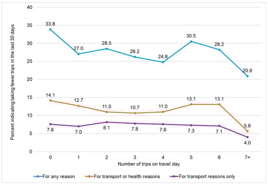
Figure 1.
Proportions of 2022 NHTS respondents aged 18+ taking fewer-than-planned trips in the last 30 days by number of trips taken on the travel day.
A detailed discussion on travel need has been provided in Section 2.3. Suffice to say at this stage that the logit models predicting trip deprivation for various reasons account for variations in travel need through the integration of a latent variable representing travel need. That variable was obtained through a confirmatory factor analysis (CFA) which used variables that are theoretically likely to affect travel need but are not likely to be affected by travel need or actual travel.
2. Literature Review
This literature review is divided into four sections. The first section describes how trip deprivation or unmet mobility relates to the original conceptualization of transportation disadvantage in the US. The second section relates US transportation policies to trip deprivation. The third section describes the literature related to the propensity of being trip-deprived and the consequences of trip deprivation. The fourth section includes a brief discussion on travel need. That section is included to provide some basic understanding of the topic because of the integration of a variable for travel need when empirically examining trip deprivation. There is a wide body of research on social exclusion that also relates to trip deprivation, but because most of that literature has been written in non-American contexts, a review of that literature is not included. Because the paper is exclusively about the US, the historical US literature has been given greater priority over other research.
2.1. A Historical Overview of Trip Deprivation in America
The 1960s was the decade when certain people’s inability to travel came to the attention of US transportation researchers, although the topic continued to receive attention in the 1970s and 1980s. Altshuler [6] was one of the first, if not the first, to use the term ‘transportation disadvantage’ to suggest that people with disabilities and low income could not take trips that others could; hence, they were deserving of special consideration from transit agencies. In other research of that time, the idea that some people could not make desired trips was implicit, but attempts to show people’s inability to make trips with real data were rarely made [21,22,23,24]. For some authors, like McGuire [23], the most important question was who deserved to be considered transportation-disadvantaged rather than who had encountered barriers or who had forgone trips because they could not travel.
A report by the Transportation Research Board [8] is critical to understanding which groups of the American people could be trip-deprived because of travel barriers. Although the primary focus of the report was on the travel difficulties of older adults, people with disabilities, and poor people, it also refers to travel barriers encountered by people without cars as well as people living in inner cities and rural areas. Despite identifying these population groups as disadvantaged, the report only provided national data on people belonging to some of the groups and overlaps between the groups, instead of providing data on forgone trips by the populations. Similar to the TRB study, Meyer and Gómez-Ibáñez [25] also paid special attention to poor people, older adults, and people with disabilities when discussing the transportation disadvantaged in the US but did not provide data on number of people actually forgoing trips. In addition to the aforementioned populations, women were also historically considered transportation-disadvantaged by some authors [23,26] because of their lower car ownership rate, transit dependency, and problems in balancing work and home activities.
Instead of questioning who is transportation-disadvantaged, Altshuler et al. [20] focused on the reasons for disadvantage and placed the blame squarely on the growing popularity of cars among certain groups and the expanding size of cities. They argued that the association between income and car ownership made the American transportation system inequitable, but they also pointed out that trip deprivation is not a straightforward issue that can be examined by counting how many trips people make: “The mere fact that a group averages fewer trips per capita than the national norm by no means provides adequate evidence that its members suffer from mobility deprivation” [20] (p. 257). They also added that asking people about desired trips could generate misleading results because some people may respond by thinking about the most essential trips, whereas others may respond by thinking about the trips they fancy. Thus, on the one hand, they showed the importance of considering variations in travel need, and on the other, they suggested a refrain from asking about desired trips when assessing travel deprivation.
Studies on spatial mismatch and skill mismatch in metropolitan areas are also highly relevant to provide a background on trip deprivation in America [7,27,28,29,30,31,32]. This stream of research deals with job access problems faced by central city Black workers because of increasing distance from areas experiencing job growth, low car ownership, and a skills mismatch between the people living in central cities and the jobs nearby. Many of these studies attributed poverty, unemployment, and welfare dependency among minority residents of central cities to these factors. Although these studies often provided data on the presence of spatial and skill mismatches, because of the dearth of data on trip deprivation or forgone trips, they did not demonstrate the number of people or workers who did not make trips because of the travel barriers they encountered. They instead paid attention to travel barriers such as longer commuting time, smaller job search area, and other constraints. One of the greatest contributions of the spatial mismatch literature is its emphasis on transportation issues specifically encountered by Black workers because of a historically segregated housing market and a low car ownership rate among Black people in American cities.
2.2. Transportation Policies Related to Trip Deprivation
Although government policies do not specifically mention trip deprivation or unmet mobility, they provide insights into the population groups that have received attention from transportation planning agencies because of regulatory requirements. An assessment of trip deprivation among various populations can show whether trip deprivation is equitably distributed.
The Civil Rights Act of 1964, the National Environmental Policy Act of 1969, and the Americans with Disabilities Act of 1990 have to be considered three of the most influential federal laws affecting transportation equity in the US because many other laws and regulations were subsequently founded on those laws [10,33]. The Civil Rights Act was important because its purpose was to prevent discrimination based on race, color, religion, and sex, whereas the main purpose of the Americans with Disabilities Act was to prevent discrimination against people with disabilities. The Presidential Executive Order on Environmental Justice and related orders by the US Department of Transportation, which have been highly consequential for transportation equity analysis conducted by transportation planning agencies, were founded on the National Environmental Policy Act and the Civil Rights Act. The Urban Mass Transportation Assistance Act of 1970 is also notable because it established a federal policy emphasizing equal rights of older adults and people with disabilities to use mass transit and authorized funds specifically to fund programs to aid the two groups [33].
Various equity-related Presidential Executive Orders also had a significant effect on the practice of transportation planning. For example, Executive Order No. 12898 of 1994 (Federal Action to Address Environmental Justice in Minority Populations and Low-Income Populations) and the subsequent orders by the US Department of Transportation emphasized the importance of equitable distribution of benefits and burdens from transportation investments among all people. Since then, planning agencies have been conducting various forms of analysis regarding the location of low-income and minority populations. Presidential Executive Order No. 13166 of 2000 (Improving Access to Services for Persons with Limited English Proficiency) subsequently mandated planning agencies to consider people with limited English proficiency (LEP) as another underserved population. Executive Order 13985 of 2021 (Advancing Racial Equity and Support for Underserved Communities) emphasized the need for equity by defining the term as “the consistent and systematic fair, just, and impartial treatment of all individuals, including individuals who belong to underserved communities that have been denied such treatment, such as Black, Latino, and Indigenous and Native American persons, Asian Americans and Pacific Islanders and other persons of color; members of religious minorities; lesbian, gay, bisexual, transgender, and queer (LGBTQ+) persons; persons with disabilities; persons who live in rural areas; and persons otherwise adversely affected by persistent poverty or inequality” [34] (p. 1).
2.3. Propensity and Consequences of Trip Deprivation
A substantial proportion of the studies on the propensity and consequences of trip deprivation were conducted in the context of older adults’ unmet mobility. Most were written in contexts beyond the United States. Of the large volume of research on older people’s unmet mobility, Haustein and Siren [35], Nordbakke and Schwanen [36], Scheiner [37], Siren and Hakamies-Blomqvist [38], and Villena-Sanchez and Boschmann [39] are examples. A reason for the greater attention on unmet mobility in older adults is the association among aging, disabilities, and driving cessation. As Luiu et al. [40] noted, more than one-third of the older adults globally could experience unmet mobility. Both empirical and review studies have shown that older adults’ inability to make desired trips may affect their mental and physical wellbeing.
Deka [41], Kim [42], and Kim and Ulfarsson [43] are rare studies on trip deprivation that were conducted in US contexts, but they also focused on older adults instead of the general population. For empirical analysis, Deka [41] and Kim [42] used data from independently collected surveys, whereas Kim and Ulfarsson [43] used data from the 2017 NHTS. All three studies showed that older adults in the US are not equally likely to be trip-deprived. All three studies found that older adults with low income are more likely to be trip-deprived, while Kim [42] and Kim and Ulfarsson [43] also showed that minority older adults are more likely to be trip-deprived than non-minority older adults.
Unlike the review by Luiu et al. [40], which focused specifically on the unmet mobility of older adults, a recently published review by Palm et al. [19] covered the unmet mobility of all populations. One of the most insightful conclusions of the study was that marginalized populations suppress travel to work, education, and other essential services, whereas travel suppression for non-marginalized populations occurs for leisure or recreational trips. The scope of the extensive review by Palm et al. [19], however, was broader than typical studies on trip deprivation or unmet mobility, as evident from the fact that it used the word suppression rather than deprivation and included reviews of studies that found workers refusing job offers or quitting jobs because of travel barriers (e.g., Lubin and Deka [44]). Yet, it can be argued that the populations that are trip-deprived to a higher degree are also more likely to take actions like quitting jobs because of transportation barriers. The spatial mismatch literature seems to indicate that Black workers, on average, may suppress travel more than workers belonging to other races. Because they spend more time but travel less distance when commuting to work, a greater proportion of such workers could forgo job opportunities because of travel suppression caused by inconveniences [45,46].
2.4. Travel Need
Because past studies have used the term ‘travel need’ in many different ways, there is certainly a potential for confusion. To eliminate the possibility of any confusion about the way travel need has been operationalized in this study, a brief discussion on the topic of travel need is called for. Some studies have mentioned travel need without much consideration or description of what it means [47]. In other studies [48,49,50,51,52], the term has been used to imply trips or trip characteristics rather than needs. For example, Truong et al. [51] conclude that travel needs change with age by pointing to variations in observed trip rates. Marshall et al. [50], Xie et al. [52], Brown [48], Lehtonen et al. [49], and Wang et al. [53] use the term to imply different characteristics of trips, such as purpose, frequency, travel time, or travel mode.
In the context of tourism travel, Tasci and Ko [54] (p. 21) defined travel need as “…physical, social, and psychological deprivation that may intensify into a noticeable disequilibrium for the individual, who engages in actions with utilitarian and hedonic end benefits that may be voluntarily sought in order to reach desired physical, social, and psychological states…”. Fox [55], on the other hand, conceived travel need as the need for activity participation, but his simultaneous mention of travel demand and travel need can make one wonder whether his interpretation also includes a moral component of need. That moral component of need is present in many studies on unmet mobility and transportation disadvantage—discussed in the two previous subsections.
In the current study, travel need is independent of actual trips or trip characteristics. Here, the interpretation of travel need is less philosophical than that of Tasci and Ko [54], but not free of abstractness. It resembles Fox’s [55] interpretation in that travel need is mostly an out-of-home activity participation need, but it does not have a moral component. The methodology for estimating travel need in the current study is similar to that of Tasci and Ko [54] in that both studies used CFA. However, the context of the current study is different, and the considerations of the past study, such as social affiliation, success, excitement, surprise, etc., are irrelevant for the current study because it is not about tourism travel. Additional details about the interpretation of travel need in the current context is provided in Section 3.2.
2.5. Synopsys of Literature Review
The literature review covered four different streams of research to provide a context for this paper as well as to justify its methodology. One of the most important takeaways from the review is that historically, certain populations were considered to be transportation-disadvantaged based on the assumption that they could not make trips like others. Most notable among them were people with disabilities, people with low income, and older adults. A wide body of research also discussed the potential adverse effects of transportation disadvantage. Although it had been hypothesized that the transportation-disadvantaged populations encountered transportation barriers more than others, it was difficult to demonstrate that they were more likely to forgo planned trips for lacking transportation. One of the difficulties in the past was that the reasons for people not making trips were not known, and without that knowledge, it was difficult to distinguish the people who did not make trips because of constraints from the people who did not make trips out of choice. The 2022 NHTS finally provided an opportunity to make that distinction and identify the populations that are more likely to forgo planned trips because of transportation (and household) constraints. People’s inability to make planned trips also depends on their travel needs. It is, therefore, important to control variations in travel need when examining the likelihood of people with diverse socioeconomic characteristics forgoing planned trips.
3. Data and Methods
3.1. Data Description
Although the 2022 NHTS Version 1.0 data were released in November 2023, this paper uses slightly updated data from Version 2.0, released in February 2024. The national sample dataset includes information for 16,997 persons aged 5 years or older (age 5+) belonging to 7893 households. People living in group quarters are excluded. The dataset also includes a file containing detailed information for 31,074 trips made by the persons in the person file. The national sample dataset from the 2022 Survey is significantly smaller than the 2009 and 2017 Surveys. For example, the national samples in the 2009 and 2017 Surveys included 25,510 and 26,099 households compared with 7893 households in the 2022 Survey.
The analyses in this paper are conducted mostly by using the information from the person file, where many of the household characteristics are attached to the persons. However, a few variables were also extracted from the household file because they were not included in the person file. Each file includes weights that correct sampling bias and inflate the data to the US national population. Although the person file includes three weights, this paper uses the standard 7-day weight (named WTPERFIN by the NHTS), which was also included in the previous rounds of the survey. Because direct application of that weight leads to almost all variables being significant in multivariate models due to the inflation of the sample, a revised weight was developed following Deka and Fei [56]. That weight is essentially a scaled-down version of the original weight that corrects the sampling bias but does not inflate the sample to national population. The new weight, referred to as the revised weight hereafter, was calculated for all observations by multiplying WTPERFIN by the ratio of sample size (n) to population size (N).
Although NHTS data are available for people aged 5+ for most variables, the lower limits are not identical for all variables. In the 2022 dataset, the reasons for not making any trip on travel day are available for all people aged 5+, whereas the data on making fewer-than-planned trips in the past 30 days are available for people aged 16+. Consistent with census data, worker status is also available for people aged 16+. For greater uniformity, all analyses in this paper are conducted by restricting the dataset to people aged 18+ because people 18 and over are generally considered adults. The restriction of the survey sample from 5+ to 18+ decreased the sample size from 16,997 to 13,956.
The top part of Table 1 shows how many respondents took fewer-than-planned trips in the past 30 days. As shown in the table, whether a person took fewer trips is known for 13,921 of the 13,956 respondents. Out of them, 3970 (28.4%) reported making fewer trips, and 9951 (71.3%) reported not making fewer trips. It could not be ascertained whether the remaining 36 respondents took fewer trips (0.3%).

Table 1.
Respondents making fewer trips in the past 30 days and the reasons for making fewer trips.
As shown in the top part of Table 2, a total of 10,341 (74.1%) out of the 13,956 respondents made at least one trip on the travel day, and 3615 (25.9%) made no trips. However, among the people who did not make any trip, the reasons for not making trips are available for only 2127 people (15.2% of 13,956). For the remaining 1488 (10.7%), data on reasons could not be ascertained from the survey responses, or the respondents did not know or preferred not to respond.
Table 2.
Respondents not taking trips on the travel day and the reasons for not taking trips.
The responses of the 13,956 people aged 18+ to the questions inquiring about the reasons for making fewer trips in the past 30 days are presented in Table 1. The responses to the question on the reasons for not making any trip on the travel day are presented in Table 2. Both sets of responses are derived by applying the revised weight, for which the percentages are the same as they would be if the original weight attached to the dataset were used, but the number of respondents reflect the sample rather than the population. It should be noted that the percentages for the reasons for making fewer trips in the past 30 days are derived from a question that allowed for the selection of multiple reasons, whereas the percentages for the reasons for not making any trip on the travel day are derived from a question that allowed only a single selection. Hence, the percentages in the two tables cannot be compared, but the percentages for reasons within the same table are comparable.
Table 1 shows that 10 reasons were given to the responses to select from when they were asked about not making trips in the past 30 days. The reasons numbered 2 through 6 in the table more clearly relate to perpetual transportation constraints (lack of safety, cleanliness, reliability, availability, and affordability) than the other reasons. Reason 7, especially health problems, can also be perceived as a transportation constraint, because both legally and morally, people with disabilities are considered transportation-disadvantaged. Reason 8—not having time to travel—is ambiguous and hence difficult to interpret. For example, one person may have no time to travel because they plan to spend the day sunbathing, and another person may not have time because they need to take care of a sick parent. Reason 9—“concerns related to COVID-19”—was certainly important during and immediately after the pandemic, but it is not a perpetual transportation issue like reliability or affordability. Reason 10, “another reason” (i.e., something else), is obviously too ambiguous, and it is impossible to know what types of constraints the respondents had, if any. Finally, Reason 1—having home deliveries—is difficult to interpret as a constraint because if a respondent selecting that reason acquired something from somewhere, the home delivery relinquished the person’s need to travel. Based on the above observations, it was decided that three variables could be generated for multivariate analysis, the first representing all respondents who selected any of the ten reasons in Table 1, the second representing reasons 2 to 6 (transportation reasons only), and the third representing reasons 2 to 7 (transportation and health reasons). In the first case, out of the 13,921 people with valid data, 3970 made fewer trips for any of the ten reasons in Table 1, whereas the other 9951 did not make fewer trips. In the second case, 1072 people selected one or more of reasons 2 to 6, whereas the other 12,849 did not select any of those reasons. In the third case, 1614 people selected one or more of reasons 2 to 7, while the other 12,301 did not select any of those reasons. Note that aggregating the number of respondents in Table 1 will not generate these numbers because a single respondent could select more than one response (e.g., a respondent selecting reasons 2, 4, and 5 is still one person).
In Table 2, where the responses to the question on not making any trip on the travel day are shown, only reason 10—“No transportation available”—directly relates to transportation. However, only 56 respondents selected that option. Reasons 3 and 4, representing caretaking and disability, can also be considered long-lasting constraints based on moral grounds. Being personally sick or quarantining (reason 1) and being hospitalized or being otherwise confined (reason 12) are certainly constraints, but whether those reasons reflect long-term or short-term ailments is difficult to know. Regarding reason 7, household chores can be more easily conceived as a constraint than projects. Household projects are difficult to interpret as a constraint because the opportunity costs of the projects are not known. For example, if a person’s project is renovation of their dwelling, it is difficult to interpret the project as a constraint. Additionally, a connection between personal transportation and such projects is difficult to comprehend. All other reasons in Table 2 are also difficult to interpret as constraints. Based on the implications of all the reasons in the context of transportation, it was decided that reason 10 (“No transportation available”) could be a variable by itself for further analysis even though only 56 respondents selected that reason. Another variable of interest could be one that combines reason 10, reason 3 (“Caretaking”), and reason 4 (“Disabled or home-bound”). A total of 219 respondents selected one of those three reasons. Although reason 1 (“Personally sick or quarantining”) and reason 12 (“Hospitalized or otherwise confined”) also reflect constraints, they were not included with the assumption that the constraints are temporary. Because these two reasons reflect constraints, but it is not known whether they reflect long-term or short-term ailments, they were excluded from analysis (similar to those who refused to respond or did not know the answer). Thus, the total number of observations excluded from the analysis of people making no trips on travel day for transportation and/or disability and caretaking reasons is 1667.
3.2. Methods
Three binary logit models were used to compare the 2022 NHTS respondents who took fewer-than-planned trips in 30 days with others. The first compared the respondents who took fewer trips for transportation reasons only (reasons 2 to 6 in Table 1), the second compared the respondents who took fewer trips because of transportation or health reasons (reasons 2 to 7 in Table 1), and the third compared all respondents who took fewer trips for any reason (reasons 1 to 10 in Table 1). In all cases, the stated categories were coded 1, whereas others were coded 0, meaning that the models predicted the likelihood of a respondent belonging to the stated categories.
Three similar models were used to compare the respondents who did not take any trip on the travel day. The first compared the respondents who did not take any trip because of the unavailability of transportation (reason 10 in Table 2), the second compared the respondents who did not take any trip because of transportation unavailability, caretaking, or disability (reason 3, 4, or 10 in Table 2), and all respondents who did not take any trip (reasons 1 to 15 of Table 2). Similar to the models on taking fewer trips, the three models predicted the likelihood of a respondent belonging to the stated categories.
Three categories of explanatory variables were included in the logit models: person-related, household-related, and geography-related. The inclusion of geographic explanatory variables was important because, on the one hand, they can inform transportation planners about which types of areas deserve more attention for transportation improvements, and on the other, they help to control for geographic variations when examining the relation between people’s characteristics and trip deprivation. Some geographic variables, such as metropolitan area designation and population size, as well as urban–rural distinction, are already included in the 2022 NHTS dataset. A variable for residence type (detached, apartment, etc.) also provides insight into the nature of the residential location of the respondents. However, unlike the 2017 NHTS, even Version 2.0 of the 2022 NHTS, released in March 2024, does not include any variable for population or job density at the census tract or census block group level. The author’s correspondence with an NHTS official revealed that it was still uncertain whether those variables would be integrated with the NHTS data in the future. Based on that understanding, population density at the block group level and job density at the census tract level were imputed from the 2017 NHTS data.
The explanatory variables of the logit models, presented in Section 4.3, were selected on the basis of the literature review, especially the literature on transportation disadvantage and spatial mismatch as well as government policies. Based on the literature, laws, and regulations, it was hypothesized that the likelihood of being trip-deprived would be higher for the respondents belonging to populations that are generally considered to be transportation-disadvantaged: people with disabilities, people with low income, people belonging to minority races and ethnicities, people speaking non-English languages, unemployed people, older adults, and women. It was also hypothesized that people with higher travel need would be more likely to be trip-deprived. Similarly, single parents and people with children generally were expected to be more trip-deprived because of the need to transport children. People from single-person households were also expected to be more trip-deprived because of the need to single-handedly take care of all household activities. People in rural areas were expected to have a higher likelihood of being trip-deprived than people living in urban areas, but people living in apartments and in areas with high population density in the residential block group were also expected to have a higher likelihood of being trip-deprived because of the socioeconomic differences between cities and suburbs. A variable for rail transit availability in the region and residence in single-family detached home were included in the models to examine if they had any relationship with the predicted variables. A variable indicating whether a person also had forgone trips on the travel day was included to examine if there is a correspondence between people who forgo trips over a period of 30 days and just 1 day. A similar (i.e., positive or negative) significant association would indicate direct correspondence between the two.
The variables on population density and job density for the 2022 households were imputed by using geographic characteristics (including metropolitan area population size, rural–urban classification, availability of rail transit in the region, and census region), as well as personal and household characteristics (including household size, number of workers in household, household income, vehicles in household, and the race of the respondent). The method involved the integration of the 2017 data (with the density variables and the predictor variables) and the 2022 data (with the predictor variable but without the density variables) and subsequently predicting the density variables. Following recommendations in Heymans and Eekhout [57], the imputed values were obtained by using the expectation maximization method instead of linear regression. With the recognition that the imputed density estimates are not exact, the predicted variables were converted to quartiles for inclusion in the models.
CFA was used to develop a latent variable representing travel need to be included in the logit models. Including a variable for travel need is important because people with higher need may have a greater likelihood of taking fewer-than-planned trips over a period of time. For example, a worker who needs to commute to work and a parent who needs to drop off children at school several days a week may have a higher travel need compared with others, and because of their higher need to make many trips, they may be more likely to forgo some trips. Although it seems intuitive to assume a positive association between travel need and number of trips one makes, need cannot be reasonably estimated from observed trips because some people with high need may not be able to travel more because of constraints. Furthermore, travel need is subjective, and hence abstract.
Although it is intuitive to assume that people with higher travel need are more likely to forgo trips over a period of time, it is difficult to hypothesize the same about a person forgoing trips on a particular day. The reason is that one can also hypothesize that the people with higher travel need could be more capable and organized (e.g., a worker must go to work, and a parent must drop off children at school). Thus, the effect of travel need on trip deprivation on a single day seems less predictable than it would be over a period of time.
In the CFA, to develop the variable travel need, only personal and household characteristics were used to generate the factor scores. Variables related to driving, drivers in household, the propensity or frequency of using different travel modes, the propensity of using online shopping, etc., were avoided because they themselves could be the outcome of travel need. Only six variables were included in the CFA: a variable representing the number of children in the household, a variable representing the number of adults in the household, a dummy variable indicating worker status, a dummy variable indicating retired status, a dummy variable indicating older age (age 65+), and a dummy variable representing people with high education (bachelor’s degree or higher). It was hypothesized that the number of children, the number of adults in the household, worker status, and high educational attainment would be positively associated with high travel need, whereas retired status and older age would be negatively associated with high travel need. The CFA was undertaken by the CALIS procedure in SAS 9.4.
Following the practice in a wide body of empirical research, the CFA results were validated based on recommendations by Gefen et al. (2000). The study recommended that Goodness-of-Fit Index (GFI), the adjusted GFI (AGFI), and the Normed Fit Index (NFI) be larger than 0.90 and Root Mean Square Residual (RMR) be smaller than 0.05. The study also recommended that all variables included in the CFA be statistically significant. Based on the study’s recommendation, the standardized coefficients from the model are presented.
Analytical methods also included the computation of variance inflation factors (VIFs) of the explanatory variables to examine multicollinearity. Although Hair Jr. et al. [57] recommends the examination of multicollinearity especially when the number of observations in the dataset is small, because the latent variable travel need was created and the variables on population and job density were imputed by variables that were also expected to have a separate and independent effect on trip deprivation, multicollinearity among the explanatory variables was checked by computing the VIF of all variables. VIF is not a statistical test, but econometricians have recommended an upper limit. For example, Hair Jr. et al. [58] Kennedy [59] and suggest a value of 10, whereas Studenmund [60] suggests a value of 5. The estimated VIF values are discussed in Section 4.2.
4. Analysis and Results
4.1. Confirmatory Factor Analysis to Create a Variable Representing Travel Need
The latent variable representing travel need had to be generated first because of the need to include the variable in the logit models. Thus, CFA was undertaken at the outset by using all observations in the dataset without missing values. The results of the analysis, including the standardized coefficients, standard errors, and the p-values of the variables obtained from the CFA, are shown in Table 3 along with the variables’ means and standard deviations. The diagnostic statistics provided at the bottom of the table sufficiently meet or exceed the thresholds recommend by Gefen et al. [61]. The signs of the coefficients (e.g., negative sign for workers and a positive sign for retired persons) indicate that the latent variable generated from the CFA represents low need rather than high need. Because it is easier to comprehend high need than low need, the variable containing the factor scores was inverted by multiplying it by −1. Thus, the variable included in the logit models represents positive travel need and the coefficients of the variable will indicate whether people with higher travel need are more or less likely to be trip-deprived.
Table 3.
Results of confirmatory factor analysis (CFA) to generate variable travel need.
4.2. Logit Models Predicting Fewer-Than-Planned Trips in 30 Days
The means and standard deviations used in the logit models are presented in Table 4. The results of the three logit models predicting the likelihood of taking fewer-than-planned trips in the past 30 days are shown in Table 5, where the odds ratios and standard errors (SEs) of the variables are presented. The model diagnostics are presented at the bottom of the table for each model. The number of observations used by the models (N) is smaller than the total number of respondents aged 18+ (13,956) because of missing values of some variables included in the models. The Likelihood Ratio Chi-Square values show that the overall models are statistically significant. The −2 Log L values and the Akaike Information Criterion (AIC) values show discernible decreases with the addition of the covariates. The Pseudo R-square values are small, but they were expected to be small because of the individual-level data with large standard deviations of the explanatory variables. The concordance values—the same as C-Statistic in the absence of ties—of the first two models are identical and substantially larger than the third model. In theory, concordance can be between 50% and 100%, but in reality, it is never close to 100% [62]. Any value larger than 60% is meaningful, but in medical research, where data quality is usually better than other fields, authors suggest a value of 70% or higher [63]. However, because concordance increases little even with the inclusion of historically proven and significant explanatory variables, Cook [62] suggests paying less attention to concordance and more attention to the Likelihood Ratio, the significance of variables, and the AIC or similar criteria.
Table 4.
Description of the explanatory variables included in the logit models.
Table 5.
Logit models predicting inability to make trips in the past 30 days due to transportation reasons, transportation or health reasons, or for any reason.
The estimated VIF values of all variables included in the models were compared with the values recommended by econometricians. Among the variables shown in Table 4 and Table 5, the highest value was observed for the imputed variable representing the highest quartile of population density (5.4) followed by the variable representing rail in the MSA (5.2). All other variables in the table had values lower than 5. It is to be noted that the two imputed variables on job density (the highest and lowest quartiles) also had VIF values greater than 5 and their inclusion increased the VIFs for the other variables used for imputation. Because the job density variables were not statistically significant in any model in Table 5 and they raised the VIF values of other variables, they were omitted from all three models. For the sake of consistency between the models in Table 5 and Table 6, those two variables were also excluded from the models in Table 6.
Table 6.
Logit models predicting lack of trips on travel day due to transportation unavailability, transportation/health/caretaking, and for all reasons.
The predicted variable in all three models in Table 5 represents taking fewer-than-planned trips in 30 days, but the reasons for taking fewer trips are different for each model. From left to right, the first model predicts the likelihood of taking fewer trips for transportation reasons only, the second model predicts the likelihood of taking fewer trips for transportation or health reasons, and the third predicts the likelihood of taking fewer trips for any reason. Thus, respondents in the predicted category (i.e., survey respondents coded 1) increases sequentially from the first model to the third. The first model is of high importance when one is focused strictly on transportation barriers, whereas the second is important when one is focused on both transportation and health barriers. Because the third model includes all reasons, including having no time and waiting for home deliveries, it may be somewhat less insightful than the first two models for transportation planning and policy purposes. Furthermore, because of the inclusion of the people whose reason was “something else”, the predicted category in the third model may be less constrained than the first two models.
An odds ratio (OR) greater than 1 in Table 5 and Table 6 for a statistically significant variable indicates a positive relation between the variable and being trip-deprived, whereas an OR less than 1 indicates a negative relationship. For example, an OR of 1.865 would indicate that people representing a category are (1.865 − 1 =) 86.5% more likely to be trip-deprived, whereas an OR of 0.517 would indicate that the people representing that category are (1 − 0.517 =) 48.3% less likely to be trip-deprived. The statistical significance of each variable in Table 5 is marked by asterisks attached to the odds ratios. Significance at the 10% is also shown to indicate that a variable is close to being statistically significant but not significant by conventional standard. Although significance at the 1% level is also shown in the table, in the following discussion, reference is made mostly to 5% level because (a) it is a convention and (b) what is significant at the 1% level is also significant at the 5% level.
The models in Table 5, especially the first and the second, generally showed what was expected. The first model, where the predicted category includes those people who took fewer trips for transportation reasons only, shows that Black people, non-English speaking people, people with disabilities, single parents, unemployed people, people who did not travel on the travel day for lacking transportation, people with higher travel need, people without vehicles in the household, people with low income, people living in single-person households, people from households with children, people living in apartments, and people living in neighborhoods with high population density are more likely to take fewer-than-planned trips over a 30-day period. In contrast, people who belonged to mixed or other races, homemakers, people with high income, and people living in metropolitan areas with rail are less likely to be trip-deprived. The OR value is the largest for people who did not take trips on the travel day, indicating that there is a direct correspondence between not taking trips on the travel day and taking fewer trips in the past 30 days. The variables representing older adults, people living in rural areas, and Hispanic people were expected to be more trip-deprived than others, but they were not statistically significant.
The results of the second model—where the predicted category included the people who had taken fewer trips for transportation or health reasons rather than transportation reasons alone—are mostly similar to the first model, but the model results show some notable differences. For example, in the second model, the variables representing Black people, single parents, people with higher travel need, people with income USD 150–USD 199.9 K, and people living in apartments are not statistically significant at the 5% level. On the other hand, people living in larger metropolitan areas and neighborhoods with low population density were found to be less likely to be trip-deprived. Since the predicted category also includes people who took fewer trips for health reasons, it is not surprising that the variable disability has the highest OR among all variables in the second model.
Although the R-square and concordance values of the third model in Table 5 are noticeably lower than the values in the first two models, its variable-specific results are mostly consistent with the other two models. The most striking difference between the third model and the other models is that it shows a greater likelihood of being trip-deprived for homemakers, whereas the other two showed a lower likelihood. Another noteworthy observation is that the variable representing Black people and single parents are once again significant like the first model. Finally, the variable representing females is significant at the 5% level only in the third model.
4.3. Logit Models Predicting Not Taking Trips on Travel Day
The models predicting the likelihood of not taking any trip on the travel day are presented in Table 6. Although a variable representing the people who did not make trips on the travel day was included in the models in Table 5, a variable representing the people taking fewer trips in the past 30 days was not included in the models in Table 6 because the predicted categories in the models are much smaller. For the same reason, the variables representing the two high-income categories were also excluded and income ≥ USD 50 K was used as the reference. Because of the small number of people in the predicted category, the inclusion of the high-income categories results in a quasi-complete separation of data points, leading to questionable results. Because of these differences, a variable-to-variable numerical comparison between the two tables would be dubious.
The predicted categories for the three models in Table 6, from left to right, are the people who did not take any trip on the travel day due to transportation unavailability; the people who did not take any trip because of transportation unavailability, health issues, or caretaking responsibilities; and the people who did not take trips for any reason. Note that the category in the first model in Table 6 is more narrowly defined than the first model of Table 5, because here, the survey question was only about availability, whereas several transportation-related issues were combined for the model in Table 5 (e.g., reliability, safety, affordability, etc.). It should also be noted that the predicted category in the third model includes all people who did not take a trip on the travel day, whether or not they provided a specific reason for that. For that reason, the number of respondents used by the model is larger than the first two models.
Although the models in Table 5 and Table 6 are not defined exactly the same way, some results are fairly consistent across the models. A comparison of the first model in Table 5 and the first model in Table 6 reveals that people with disabilities, unemployed people, and people with income below USD 25,000 are more likely to take fewer-than-planned trips during a 30-day period for transportation reasons, and they are also more likely to take no trip on the travel day because of transportation unavailability. A comparison of the second and third models in the two tables shows a similar consistency for people with disabilities and unemployed people, but the variable income is not significant in the models in Table 6. The results on some other variables are also fairly consistent across the six models. For example, the variable representing Black race is positively associated with the dependent variables in four of the six models at the 5% level and at the 10% level in another model. Similarly, the variable people without cars in the household is positively associated with the dependent variable in four models at the 5% level and significant at the 10% level in another model.
In contrast to the aforementioned variables, several variables show inconsistent results when the two tables are compared. While many of the variables representing geographic area characteristics were statistically significant in Table 5, only one is significant at the 5% level across the three models in Table 6. The variable representing people who do not speak English at home showed a significant and positive relationship with the dependent variables in all three models of Table 5, but the variable is negatively associated with the dependent variable in two models of Table 6 and not significant in the third model. The variable single-person household was positively and significantly associated with the dependent variables in all three models of Table 5, but it is not significant in two models and is significant and negative in the third model of Table 6. The variable representing workers was not significant in any model in Table 5, but it shows a significant negative association with the dependent variable in two models of Table 6.
The inconsistency of the results in Table 6 with the results in Table 5 does not make the results in Table 6 less reliable because there is a difference between the nature of the two questions from which the dependent variables in the two tables were created. The question for the models in Table 5 was asked to all respondents, whereas the question from which the dependent variables for the models in Table 6 was generated was asked only to the respondents who did not make a trip on the travel day. Consider, for example, the variable representing workers in the two sets of models. It is not significant in any of the models in Table 5, but it shows a lower likelihood of forgoing trips in two models in Table 6. Because workers have the responsibility of making work trips that non-workers do not have, the negative association of the variable in Table 6 is reasonable. Similarly, the variable homemaker shows a negative association with the dependent variables in the first two models of Table 5 (i.e., they are less likely to forgo trips in 30 days), but it shows a significant and positive relationship in all three models of Table 6 (i.e., they are more likely to forgo trips on the travel day). A plausible explanation is that homemakers are less likely to make trips on any given day compared with others, and because they are less likely to make trips on any day, they are also less likely to forgo trips over a period of time. The results for workers and homemakers are consistent with the results on the variable representing travel need. Although the variable is not significant in every model, when it is significant, it is positively associated with the dependent variable in the model in Table 5 but negatively associated in the two models in Table 6. The results on variables representing workers and homemaker in Table 6 are potentially affected by the elimination of a smaller proportion of respondents making non-discretionary trips and a larger proportion of respondents making discretionary trips. That is because people typically making trips for non-discretionary purposes are less likely to skip trips on a given day, and because of that, they would also be less likely to be included in the predicted category of the models in Table 6.
5. Discussion
Although little could be known in the past about the American people who could not make trips because of transportation and other constraints, the recently released 2022 NHTS data made it possible to examine the characteristics of those people. By analyzing those data, this paper examined the characteristics of US adults who had forgone trips (a) within a 30-day period and (b) on the travel day of the survey. The results of the first set of analysis are presented in Table 5, whereas the results of the second set are presented in Table 6. The first two models in each table are more relevant for transportation planners and policy makers because they examine trip deprivation under constraints. The third model is less useful in both tables because many of the cited reasons do not necessarily reflect constraints.
The models predicting the likelihood of taking fewer-than-planned trips in 30 days, presented in Table 5, are more meaningful than the models predicting people not taking trips on the travel day, presented in Table 6. The models in Table 6 are less meaningful because the question that generated the data was asked only to the people who did not travel on a single day. When people are restricted to only those who did not travel on a given day and then asked why they did not travel, the people who make non-discretionary trips (e.g., workers going to work and parents dropping off children at school) are more likely to be excluded from the question on reasons because they are more likely to make daily trips than others. However, when all people are asked about taking fewer-than-planned trips over a period of time—as in the question about forgoing trips in the past 30 days, the respondents are not similarly censored.
The NHTS question on the reasons for not traveling on the travel day is still useful because it allows for a comparison of the responses to the responses to the question on taking fewer-than-planned trips in 30 days. That is because a consistency between the responses of the two questions can add credence to the responses to the question about taking fewer trips over a period of time. For example, if people with disabilities are found to have a higher likelihood of forgoing trips in a 30-day period and also on the survey’s travel day, it becomes almost a certainty that people with disabilities forgo trips more than others.
The analyses in this paper demonstrated that the assumptions in the literature on transportation disadvantage and spatial mismatch, as well as the premises of the federal policies, are mostly valid. For example, the higher likelihood of trip deprivation for transportation reasons among people with disabilities, unemployed people, people speaking non-English languages at home, people with low income, and Black people—shown by the first model in Table 5—confirms that these populations are truly transportation-disadvantaged. In the second model of the table, where health constraints were added to transportation constraints, all of these populations except Black people were again found to be trip-deprived. The negative association between car ownership and the likelihood of trip deprivation in the first two models of Table 5 shows that the researchers who have attributed variations in car ownership to transportation disadvantage [20,64,65,66] have a valid argument. The first two models of Table 5 also show that people from single-person households as well as people from households with children are more likely to be trip-deprived than others.
The populations that were expected to be trip-deprived because of transportation constraints but were not found to be trip-deprived are Hispanics, females, and older adults. The results on Hispanics are perhaps not very surprising because of diversity within the group. The results on females are mixed. The first model of Table 5 shows females having a higher likelihood of being trip-deprived for transportation reasons, but only at the 10% level of significance. The third model of the same table, which predicts people taking fewer trips for any reason, shows a higher likelihood for females at the 5% level. The third model of Table 6 shows similar results. These results seem to indicate that women are more likely to forgo trips than men, but the reason for that cannot be clearly attributed to transportation.
The variable older adults, defined as people aged 65+, was not significant in any of the six models in Table 5 and Table 6. The variable was not significant even when older adults were defined as people aged 75+ instead of 65+ in a separate model. However, these results do not necessarily refute the fact that many older adults are trip-deprived. A reason for the variable older adults not being significant is the overlap between people who have disabilities and people who are old. At least two US studies [41,42] showed that older adults are highly heterogeneous. While many older adults cannot travel like others because of disabilities and low income, others are fully capable of traveling when they wish. The results of this study indicate that public policy and future research on older adults’ transportation barriers should recognize this heterogeneity.
The results also show the importance of considering racial and ethnic minorities to be heterogenous. The variable representing Black people is positively associated with the dependent variable at the 5% level in the first and the third model of Table 5, whereas the variables representing Asian people and Hispanic people are not significant in any of the three models. The variable representing mixed race and other races is significant with a negative sign in the first two models of Table 5, indicating that they are less likely to be trip-deprived. This shows, once again, that considering all minorities together as transportation-disadvantaged ignores the fact that the Black population is more disadvantaged than other minorities in terms of trip deprivation.
A number of place-related variables are significant in the models in Table 5. The variable representing high population density in the neighborhood has a significant and positive association with trip deprivation in all three models of the table, indicating that people living in neighborhoods with high density are more likely to be trip-deprived. That could be because neighborhoods with high population density are often inhabited by low-income, Black, and carless households. The positive relationship of the variable representing people living in apartments in the first model of Table 5 is consistent with the results on population density because the high-density areas typically contain a larger share of apartments. These results show that transportation policy should pay significantly greater attention to central city areas with high population density.
Although one could be surprised to see that rural residents are not more likely to be trip-deprived than others, it is perhaps not surprising because the comparison category is people living in urban areas, where many people live without cars. Just because trip deprivation of rural residents is not higher, one should not conclude that they do not encounter other transportation barriers. One of the most obvious barriers for rural residents is the distance they have to travel between activity sites.
The variable representing rail transit in metropolitan areas is significantly and negatively associated with the dependent variables of all three models in Table 5, indicating that the likelihood of being trip-deprived is lower in metropolitan areas served by rail. However, it is difficult to conclude from this association that rail transit has any effect on reducing trip deprivation because rail transit in US cities is commonly used by people with high income. It is perhaps more reasonable to conclude from the observed association that rail is more likely to be available in areas where people have lower trip deprivation because of affluence.
Although the primary objective of this paper is to identify populations that are more likely to be trip-deprived than others, certain theoretical and practical recommendations can be made for addressing trip deprivation and its effects. In the theoretical domain of transportation equity, researchers lately have been arguing in favor of operationalizing the Capability Approach (CA), a detailed review of which can be found in van Burgsteden et al. [67]. Most studies seeking the implementation of the CA suggested both land use strategies and transportation strategies. Between the two types of strategies, the latter would be more effective to address trip deprivation because transportation improvements usually have a more direct and immediate effect on mobility than land use improvements. However, the CA also demands that people choose beneficial strategies themselves, meaning that strategies to address trip deprivation should be selected by a bottom-up approach. That would require substantial public engagement.
The initial strategies to address transportation disadvantage in this country evolved around public transportation. For example, the subsidization of transit trips by people with disabilities and older adults was one of the earliest strategies. However, despite making technological progress by providing real-time information and allowing online ticketing, transit agencies still offer services mostly by trains and fixed-route buses in high-density urban areas. Due to the decentralization of activities over the past decades, fixed-route transit cannot effectively serve trip-deprived individuals who live in transit-poor areas or those whose typical destinations are not served by buses and trains. Even within high-density areas, fixed-route transit does little to serve certain traditionally deprived populations like older adults [41]. The provision of variable-route and door-to-door service with smaller vehicles in addition to fixed-route transit could address the issue somewhat. Other strategies could be a collaboration between transit agencies and ridehailing companies and means-tested subsidization of ridehailing trips. In recent years, researchers have been increasingly arguing in favor of greater car access for underserved populations [64,66]. App-based car rental practices could potentially be expanded.
The effects of trip deprivation could be addressed by recent improvements in information and communication technologies (ICTs) as well as app-based transportation technologies [68]. Greater flexibility for workers to work from home could provide relief to those who have difficulty commuting. Technologies like telemedicine, online shopping, and videoconferencing have already become popular. Ridehailing has also acquired a reasonable share of the travel market. There is an expectation among researchers like Golant [68] that autonomous vehicles (AVs) will provide another travel option in the future to people who cannot drive. However, modern technologies will be beneficial to people with low income only if their costs are affordable. Expanded subsidization of childcare could provide relief to parents with children who cannot make planned trips because of childcare responsibilities [69]. Thus, in addition to transportation policies and strategies, modern technologies and government policies could help to address the effects of trip deprivation. That is not to suggest that trip deprivation and its effects could not be addressed by improving conventional fixed-route transit. Certain transit agencies are already undertaking projects like bus network redesign with consideration of the residential location of traditionally underserved populations. Those efforts could be improved through collaborative efforts between MPOs and transit agencies to identify trip-deprived populations. Access to stations/stops could also be improved.
It ought to be noted that the results of this research are pertinent to the US as a whole and may not be directly applicable to a specific metropolitan area. In addition to the national sample, the 2022 NHTS also collected data through oversampling for certain areas. Metropolitan planning organizations (MPOs) in regions for which such data were collected can conduct analyses similar to this research to learn about trip deprivation in their own regions. Other MPOs could include questions on trip deprivation in their own household travel surveys for similar analyses.
The NHTS does not include questions seeking recommendations for addressing trip deprivation. Such questions are not highly valuable in a national survey because the recommendations may vary from one region to another. However, MPOs could include such questions in their own household travel surveys and analyze the responses at the subregional level to determine what types of transportation improvement strategies may be applicable to which part of the region.
Funding
This research received no external funding.
Institutional Review Board Statement
Not applicable.
Informed Consent Statement
Not applicable.
Data Availability Statement
Data are contained within the article.
Conflicts of Interest
The authors declare no conflict of interest.
References
- Boström, M. A Missing Pillar? Challenges in Theorizing and Practicing Social Sustainability: Introduction to the Special Issue. Sustain. Sci. Pract. Policy 2012, 8, 3–14. [Google Scholar] [CrossRef]
- Murphy, K. The Social Pillar of Sustainable Development: A Literature Review and Framework for Policy Analysis. Sustain. Sci. Pract. Policy 2012, 8, 15–29. [Google Scholar] [CrossRef]
- Nilsson, C.; Levin, T.; Colding, J.; Sjöberg, S.; Barthel, S. Navigating Complexity with the Four Pillars of Social Sustainability. Sustain. Dev. 2024, 1–19. [Google Scholar] [CrossRef]
- Agyeman, J. Toward a ‘Just’ Sustainability? Continuum 2008, 22, 751–756. [Google Scholar] [CrossRef]
- Agyeman, J.; Bullard, R.D.; Evans, B. Exploring the Nexus: Bringing Together Sustainability, Environmental Justice and Equity. Space Polity 2002, 6, 77–90. [Google Scholar] [CrossRef]
- Altshuler, A. Transit Subsidies: By Whom, for Whom? J. Am. Inst. Plan. 1969, 35, 84–89. [Google Scholar] [CrossRef]
- Kain, J.F. Housing Segregation, Negro Employment, and Metropolitan Decentralization. Q. J. Econ. 1968, 82, 175–197. [Google Scholar] [CrossRef]
- TRB (Transportation Research Board). Transportation Requirements for the Handicapped, Elderly, and Economically Disadvantaged; National Cooperative Highway Research Program Synthesis of Highway Practice, Transportation Research Board: Washington, DC, USA, 1976. [Google Scholar]
- FHWA (Federal Highway Administration). 2022 NextGen National Household Travel Survey Core Data; U.S. Department of Transportation: Washington, DC, USA, 2022.
- Deka, D. Environmental Justice, Transport Justice, and Mobility Justice. Int. Encycl. Transp. 2021, 7, 305–310. [Google Scholar] [CrossRef]
- FHWA and FTA (Federal Highway Administration & Federal Transit Administration). The Metropolitan Transportation Planning Process: Key Issues; Report No. FHWA-EP-03-041 (5/04); U.S. Department of Transportation: Washington, DC, USA, 2004.
- Sciara, G.C. Metropolitan Transportation Planning: Lessons from the Past, Institutions for the Future. J. Am. Plan. Assoc. 2017, 83, 262–276. [Google Scholar] [CrossRef]
- Karner, A.; London, J.; Rowangould, D.; Manaugh, K. From Transportation Equity to Transportation Justice: Within, Through, and Beyond the State. J. Plan. Lit. 2020, 35, 440–459. [Google Scholar] [CrossRef]
- Martens, K.; Golub, A.; Robinson, G. A Justice-Theoretic Approach to the Distribution Of Transportation Benefits: Implications for Transportation Planning Practice in the United States. Transp. Res. Part A Policy Pract. 2012, 46, 684–695. [Google Scholar] [CrossRef]
- Martens, K. Transport Justice: Designing Fair Transportation Systems; Routledge: Oxfordshire, UK, 2017. [Google Scholar]
- Sheller, M. Mobility Justice: The Politics of Movement in an Age of Extremes; Verso: London, UK, 2018. [Google Scholar]
- FHWA (Federal Highway Administration). 2009 National Household Travel Survey; U.S. Department of Transportation: Washington, DC, USA, 2009.
- FHWA (Federal Highway Administration). 2017 National Household Travel Survey; U.S. Department of Transportation: Washington, DC, USA, 2017.
- Palm, M.; Nakshi, P.; Barri, E.Y.; Farber, S.; Widener, M. Uncovering Suppressed Travel: A Scoping Review of Surveys Measuring Unmet Transportation Need. Travel Behav. Soc. 2024, 36, 100784. [Google Scholar] [CrossRef]
- Altshuler, A.; Womack, J.P.; Pucher, J.R. The Urban Transportation System: Politics and Policy Innovation; MIT Press: Cambridge, MA, USA, 1979. [Google Scholar]
- Falcocchio, J.C.; Cantilli, E.J. Transportation and the Disadvantaged: The Poor, the Young, the Elderly, the Handicapped; Lexington Books: Lanham, MD, USA, 1974. [Google Scholar]
- Paaswell, R.E.; Recker, W.W. Location of the Carless. Transp. Res. Rec. 1974, 516, 11–20. [Google Scholar]
- McGuire, C. Who Are the Transportation Disadvantaged? Report No. DOT-BIP-WP-27-10-77; Metropolitan Transportation Commission: Berkeley, CA, USA; Department of Housing and Urban Development: Washington, DC, USA; U.S. Department of Transportation: Washington, DC, USA, 1976.
- Schnell, J.B. Public Transportation and the Needs of the Elderly and Handicapped. Transp. Res. Rec. 1974, 516, 1–10. [Google Scholar]
- Meyer, J.R.; Gómez-Ibáñez, J.A. Autos, Transit, and Cities; Harvard University Press: Cambridge, MA, USA, 1981. [Google Scholar]
- Wekerle, G.R.; Rutherford, B.M. Employed Women in the Suburbs: Transportation Disadvantage in a Car-Centered Environment. Alternatives 1987, 14, 49–54. Available online: http://www.jstor.org/stable/45030591 (accessed on 27 May 2024).
- Eom, H. Recent Intra-Metropolitan Patterns of Spatial Mismatch: Implications for Black Suburbanization and the Changing Geography of Mismatch. Growth Chang. 2023, 54, 421–445. [Google Scholar] [CrossRef]
- Gobillon, L.; Selod, H.; Zenou, Y. The Mechanisms of Spatial Mismatch. Urban Stud. 2007, 44, 2401–2427. [Google Scholar] [CrossRef]
- Holzer, H.J. The Spatial Mismatch Hypothesis: What has the Evidence Shown? Urban Stud. 1991, 28, 105–122. [Google Scholar] [CrossRef]
- Houston, D. Employability, Skills Mismatch and Spatial Mismatch in Metropolitan Labour Markets. Urban Stud. 2005, 42, 221–243. [Google Scholar] [CrossRef]
- Ihlanfeldt, K.R.; Sjoquist, D.L. The Spatial Mismatch Hypothesis: A Review of Recent Studies and their Implications For Welfare Reform. Hous. Policy Debate 1998, 9, 849–892. [Google Scholar] [CrossRef]
- Ong, P.; Blumenberg, E. Job Access, Commute And Travel Burden Among Welfare Recipients. Urban Stud. 1998, 35, 77–93. [Google Scholar] [CrossRef]
- Weiner, W. Urban Transportation Planning in the United States, 3rd ed.; Springer Science and Business: Berlin, Germany, 2008. [Google Scholar]
- The White House. Executive Order 13985: Advancing Racial Equity and Support for Underserved Communities through the Federal Government. Fed. Regist. 2021, 86, 14. [Google Scholar]
- Haustein, S.; Siren, A. Seniors’ Unmet Mobility Needs—How Important is a Driving Licence? J. Transp. Geogr. 2014, 41, 45–52. [Google Scholar] [CrossRef]
- Nordbakke, S.; Schwanen, T. Transport, Unmet Activity Needs and Wellbeing in Later Life: Exploring The Links. Transportation 2015, 42, 1129–1151. [Google Scholar] [CrossRef]
- Scheiner, J. Does the Car make Elderly People Happy and Mobile? Settlement Structures, Car Availability and Leisure Mobility of the Elderly. Eur. J. Transp. Infrastruct. Res. 2006, 6, 151–172. [Google Scholar] [CrossRef]
- Siren, A.; Hakamies-Blomqvist, L. Private Car as the Grand Equaliser? Demographic Factors and Mobility in Finnish Men and Women Aged 65+. Transp. Res. Part F Traffic Psychol. Behav. 2004, 7, 107–118. [Google Scholar] [CrossRef]
- Villena-Sanchez, J.; Boschmann, E.E. A Scoping Review of the Daily Mobilities of Older Adults in the Global South. Can. Geogr. 2022, 66, 119–131. [Google Scholar] [CrossRef]
- Luiu, C.; Tight, M.; Burrow, M. The Unmet Travel Needs of the Older Population: A Review of the Literature. Transp. Rev. 2017, 37, 488–506. [Google Scholar] [CrossRef]
- Deka, D. Trip Deprivation Among Older Adults in the Context of the Capability Approach. J. Transp. Geogr. 2022, 100, 103325. [Google Scholar] [CrossRef]
- Kim, S. Assessing Mobility in an Aging Society: Personal and Built Environment Factors associated with Older People’s Subjective Transportation Deficiency in the US. Transp. Res. Part F Traffic Psychol. Behav. 2011, 14, 422–429. [Google Scholar] [CrossRef]
- Kim, S.; Ulfarsson, G.F. Staying Home or Going Places: Mobility Factors of Older Minority Women’s Daily Trip Making in the United States. J. Transp. Health 2021, 21, 101031. [Google Scholar] [CrossRef]
- Lubin, A.; Deka, D. Role of Public Transportation as Job Access Mode: Lessons from Survey of People with Disabilities in New Jersey. Transp. Res. Rec. 2012, 2277, 90–97. [Google Scholar] [CrossRef]
- Deka, D. Social And Environmental Justice Issues in Urban Transportation. In The Geography of Urban Transportation; Hanson, S., Giuliano, G., Eds.; The Guilford Press: New York, NY, USA, 2004; pp. 332–355. [Google Scholar]
- Giuliano, G. Travel, Location and Race/Ethnicity. Transp. Res. Part A Policy Pract. 2003, 37, 351–372. [Google Scholar] [CrossRef]
- Sihvola, T.; Jokinen, J.P.; Sulonen, R. User Needs for Urban Car Travel: Can Demand-Responsive Transport Break Dependence on the Car? Transp. Res. Rec. 2012, 2277, 75–81. [Google Scholar] [CrossRef]
- Brown, A. Redefining Car Access: Ride-hail Travel and Use in Los Angeles. J. Am. Plan. Assoc. 2019, 85, 83–95. [Google Scholar] [CrossRef]
- Lehtonen, E.; Malin, F.; Louw, T.; Lee, Y.M.; Itkonen, T.; Innamaa, S. Why would People want to Travel More with Automated Cars? Transp. Res. Part F Traffic Psychol. Behav. 2022, 89, 143–154. [Google Scholar] [CrossRef]
- Marshall, S.; Banister, D.; McLellan, A. A Strategic Assessment of Travel Trends and Travel Reduction Strategies. Innov. Eur. J. Soc. Sci. Res. 1997, 10, 289–304. [Google Scholar] [CrossRef]
- Truong, L.T.; De Gruyter, C.; Currie, G.; Delbosc, A. Estimating the Trip Generation Impacts of Autonomous Vehicles on Car Travel in Victoria, Australia. Transportation 2017, 44, 1279–1292. [Google Scholar] [CrossRef]
- Xie, C.; Boyles, S.D.; Dong, J.; Wu, X. Travel Behavior and Transportation Systems Analysis of Electric Vehicles. J. Adv. Transp. 2018, 2018, 1–2. [Google Scholar] [CrossRef]
- Wang, W.; Espeland, S.; Barajas, J.M.; Rowangould, D. Rural–nonrural Divide in Car Access and Unmet Travel Need in the United States. Transportation 2023, 1–30. [Google Scholar] [CrossRef]
- Tasci, A.D.; Ko, Y.J. Travel Needs Revisited. J. Vacat. Mark. 2017, 23, 20–36. [Google Scholar] [CrossRef]
- Fox, M. Transport Planning and the Human Activity Approach. J. Transp. Geogr. 1995, 3, 105–116. [Google Scholar] [CrossRef]
- Deka, D.; Fei, D. A Comparison of the Personal and Neighborhood Characteristics Associated with Ridesourcing, Transit Use, and Driving with NHTS Data. J. Transp. Geogr. 2019, 76, 24–33. [Google Scholar] [CrossRef]
- Heymans, M.W.; Eekhout, I. Applied Missing Data Analysis with SPSS and ®Studio; Heymans and Eekhout, Amsterdam, The Netherlands. 2019. Available online: https://bookdown.org/mwheymans/bookmi/ (accessed on 23 February 2024).
- Hair, J.F., Jr.; Black, W.C.; Babyn, B.J.; Anderson, R.E. Multivariate Data Analysis, 7th ed.; Pearson Education Limited: London, UK, 2014. [Google Scholar]
- Kennedy, P. A Guide to Econometrics, 4th ed.; The MIT Press: Cambridge, MA, USA, 2001. [Google Scholar]
- Studenmund, A.H. Using Econometrics: A Practical Guide, 4th ed.; Addison Wesley: London, UK, 2021. [Google Scholar]
- Gefen, D.; Straub, D.; Boudreau, M. Structural Equation Modeling and Regression: Guidelines for Research Practice. Commun. Assoc. Inf. Syst. 2000, 4, 7. [Google Scholar] [CrossRef]
- Cook, N.R. Use and Misuse of the Receiver Operating Characteristic Curve in Risk Prediction. Circulation 2007, 115, 928–935. [Google Scholar] [CrossRef] [PubMed]
- Mandrekar, J.N. Receiver Operating Characteristic Curve in Diagnostic Test Assessment. J. Thorac. Oncol. 2010, 5, 1315–1316. [Google Scholar] [CrossRef] [PubMed]
- Klein, N.J. Subsidizing Car Ownership for Low-income Individuals and Households. J. Plan. Educ. Res. 2024, 44, 165–177. [Google Scholar] [CrossRef]
- Ong, P.M.; Miller, D. Spatial and transportation mismatch in Los Angeles. J. Plan. Educ. Res. 2005, 25, 43–56. [Google Scholar] [CrossRef]
- Smart, M.J.; Klein, N.J. Disentangling the Role of Cars and Transit in Employment and Labor Earnings. Transportation 2020, 47, 1275–1309. [Google Scholar] [CrossRef]
- van Burgsteden, M.; Grigolon, A.; Geurs, K. Improving Community Wellbeing through Transport Policy: A Literature Review and Theoretical Framework, Based on the Capability Approach. Transp. Rev. 2024, 1–26. [Google Scholar] [CrossRef]
- Golant, S.M. Stop Bashing the Suburbs: Mobility Limitations of Older Residents are Less Relevant as Connectivity Options Expand. J. Aging Stud. 2019, 50, 100793. [Google Scholar] [CrossRef] [PubMed]
- Maguire-Jack, K.; Park, Y.; Feely, M.; Schneider, W.; Pace, G.T.; Klika, J.B.; Thibodeau, E. Childcare Subsidy Employment And Copayment Requirements And Child Maltreatment. Child Maltreatment 2023, 10775595231218174. [Google Scholar] [CrossRef] [PubMed]
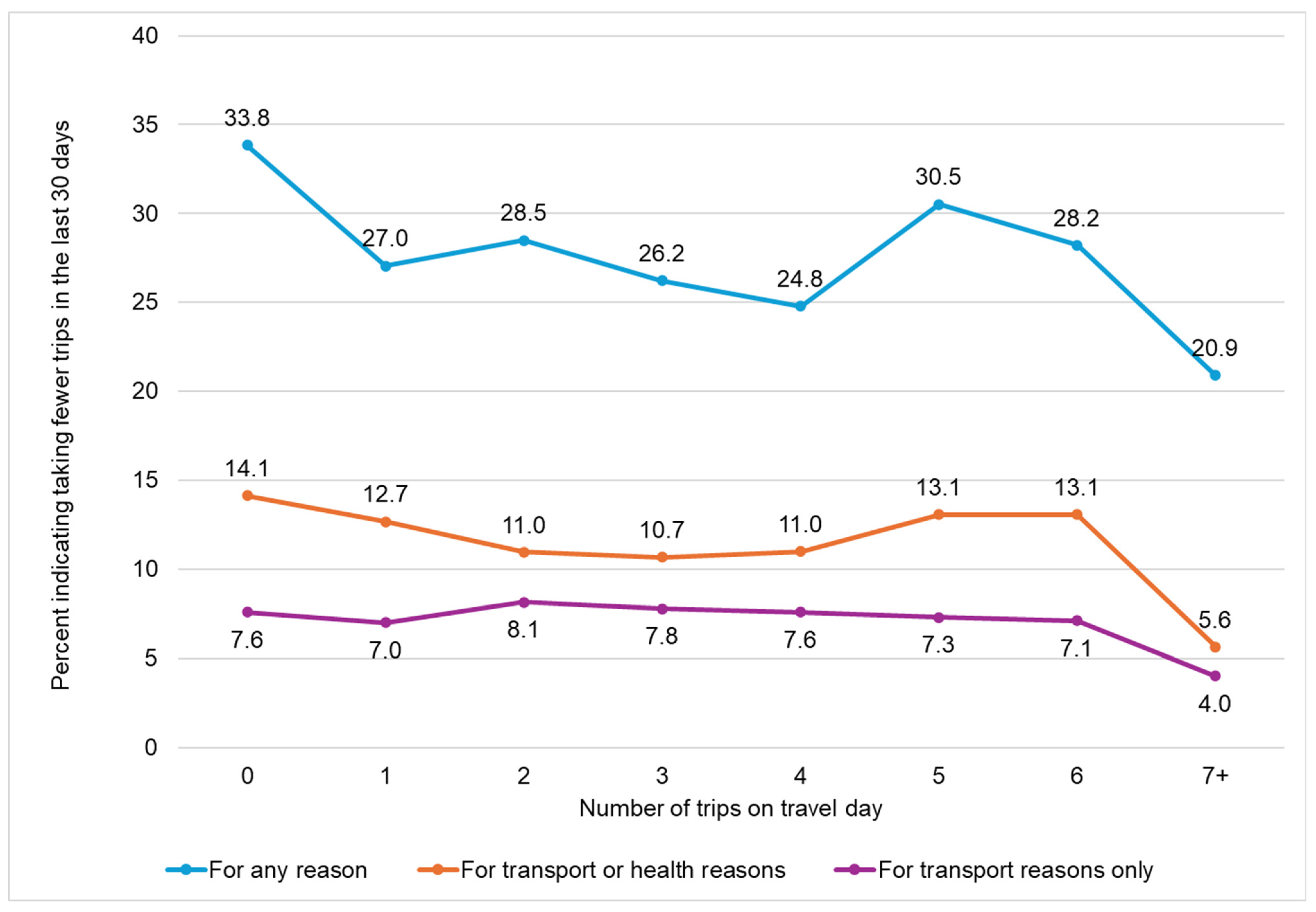
Disclaimer/Publisher’s Note: The statements, opinions and data contained in all publications are solely those of the individual author(s) and contributor(s) and not of MDPI and/or the editor(s). MDPI and/or the editor(s) disclaim responsibility for any injury to people or property resulting from any ideas, methods, instructions or products referred to in the content. |
© 2024 by the author. Licensee MDPI, Basel, Switzerland. This article is an open access article distributed under the terms and conditions of the Creative Commons Attribution (CC BY) license (https://creativecommons.org/licenses/by/4.0/).