Abstract
In the process of human social development, the coupling and coordinated development of ecological function (EF), production function (PF), and living function (LF) are of great significance for sustainable development. In this study, an improved coupling coordination degree model (CCDM) is used to discover the coordination conflict between EF and a human settlement environment. The main work performed in this study is as follows: (1) A more objective weight value that can avoid analysis errors caused by a subjective judgment weight value is obtained. (2) A constitutive model of EF, PF, and LF is constructed, and then resilience indicators that reflect the burden of human activities in EF are proposed. (3) We find that, during the urbanization of Ya’an city from 2014 to 2018, the degree of coupling (DOC) between EF, PF, and LF is high, but the coupling coordination degree (CCD) between the three values is low; specifically, the DOC between EF and the other two values shows the biggest decline. (4) Finally, the resilience of EF is used to explain the decrease in coordination between EF, PF, and LF, while also explaining the obvious problem of a decrease in CCD between EF and the other two values. In this study, the method for calculating the DOC and COD is optimized, and then, a theoretical model for analyzing the ecological functions bearing the pressure of human activities from qualitative and quantitative perspectives is proposed. The research results can provide an analytical framework, path, and method for the coordinated development of “PF–LF–EF” in other regions.
1. Introduction
Ecological and environmental problems, ultimately caused by excessive exploitation and unreasonable utilization of natural resources [1], are gradually becoming a major constraint on human sustainable development [2], thus attracting widespread attention from the academic community and becoming a key issue that urgently needs to be addressed [3,4]. Scholars agree that urban development needs to be scientifically planned with EF protection in mind [5,6] so that cities can fully utilize the self-regulation and restoration capabilities of various land use types and their combinations in the face of sudden and cumulative disasters and so that the resilience of urban EF can be enhanced [7,8]. The starting point of this study is the identification of the functional coupling and coordination conflict between EF, PF, and LF during the development of human society and a proposal of corresponding explanatory models [9,10].
The relationship between an urban environment and human activities has become a global research focus. With the acceleration of urbanization, the environmental challenges that cities face are becoming more complex, prompting academics and policymakers to deepen their understanding of urban ecosystems. Existing research mainly focuses on the following aspects: first, the structure and function of an urban ecosystem, including the impact of green spaces, water bodies, and air quality on residents’ health; second, human activity patterns, such as traffic flow, land use changes, and their impact on environmental quality; third, the role of socioeconomic factors on the environment, especially the behavioral patterns and consumption habits of different groups; and finally, the effectiveness of policy and management, including urban planning and the effect of environmental protection policy implementation [11].
Although many studies have provided valuable insights into the relationship between urban environments and human activities, some significant shortcomings still exist. Firstly, challenges in data integration make it difficult to conduct interdisciplinary research, with many studies relying on isolated data sets and lacking an understanding of the integrity of urban systems. Secondly, the limitations of time and space lead to limitations in the research results, which thus result in failure to fully capture the environmental impact of the dynamic changes in a city. In addition, the lack of models on human behavior makes analyses of the response of different populations to environmental changes inadequate, affecting predictions of future trends. Finally, evaluations of the effect of policy implementation are still insufficient, and the lack of a systematic feedback mechanism limits the optimization and effectiveness of policies [12].
Insufficient research has resulted in humans only being able to observe the destruction of the ecological environment but unable to explain the reasons for the deterioration of the human living environment. There is an urgent need for an explanatory model to help humans analyze the relationship between EF, PF, and LF. Through an in-depth analysis of this subject and its shortcomings, in this paper, we aim to provide a more comprehensive perspective for studying an urban environment and its human activities and to promote practical and theoretical research on sustainable urban development.
2. Literature Review
Firstly, a literature review is conducted on the resilience models, followed by a review of human activities and living functions and, finally, an analysis of the feasibility and progressiveness of applying a neural network and an average influence value algorithm to determine the weight value of each influencing factor. The coupling coordination and model evolution between EF, PF, and LF discussed in this paper are then reviewed on a long time series and multiple time scales.
2.1. Review of Ecological Environmental Resilience
In the natural sciences, the concept of resilience can be traced back to Holling’s discussion on the resilience and stability of ecosystems. The concept of resilience in the traditional ecological literature describes the persistence or plasticity of natural systems in response to changes in external natural and human factors, including two different definitions. The first definition focuses on the stability of specific adjacent equilibrium states, whose properties are quantified by their resistance to disturbances and the speed of recovery to their original equilibrium state [13]. The second definition emphasizes instability, which refers to the conditions required to trigger a system to transition from one state to another, and its properties are measured by the magnitude of the disturbance that triggers a sudden change in the equilibrium state of the system [14].
However, as an emerging research topic, no broad consensus on the concept of ecological resilience has been reached in the academic community, and not much research has been conducted on the evaluation of ecological resilience [15]. In 2001, Holling first applied the concept of ecosystem resilience to the study of urban social systems in his book Chaos: Understanding Transformations in Human and Natural Systems, proposing an “adaptive cycle” model to characterize the feedback and negative feedback mechanisms of urban “social-ecological systems” under stress and their resilience changes. The resilience of EF involves the interaction of multiple departments, industries, and factors [16]. The impact of various driving factors on ecological resilience in different regions also varies. However, the existing research focuses primarily on evaluating influencing factors from a global perspective, and research on spatiotemporal differences in the same influencing factor has not yet been conducted in-depth [17].
2.2. Review of Human Activities and Living Functions
In recent years, the relationship between human activities and urban life functions has received extensive attention. As centers of human activity, cities not only serve economic, social, and cultural functions but also have a profound impact on environmental sustainability. Earlier studies mainly focused on the impact of urbanization on land use and traffic flow [18]. These studies shed light on the environmental challenges posed by urban sprawl, such as greenhouse gas emissions and ecological damage.
In studies on urban life function, emphasis is placed on the diversity and inclusiveness of urban spaces [19]. This theory emphasizes the versatility of an urban environment and specifically emphasizes public spaces and social interactions. Furthermore, recent studies have gradually turned to assessments of urban ecosystem services [20], revealing the importance of urban green spaces and water bodies to residents’ well-being.
However, some shortcomings still persist in the existing research. First, although qualitative analyses of urban function are relatively abundant, quantitative research is relatively insufficient, especially studies assessing the specific impact of human activities on the environment. Secondly, many studies fail to effectively consider the impact of socioeconomic differences on urban functions, which leads to a one-sided understanding of urban quality of life [21]. In addition, research on the adaptation of human activities in the process of urban transformation is relatively lacking, especially in the context of climate change.
In summary, although existing research has provided an important basis for understanding human activity and the function of urban life, quantitative analyses, interdisciplinary collaborations, and comprehensive consideration of socioeconomic factors are needed in the future to promote a more comprehensive research framework.
2.3. Overview of Artificial Neural Network Models
To grasp the development pattern of land use resource changes in a certain region, a model can be constructed between a certain indicator in the region and the relevant factors affecting land use area changes. For example, Liu et al [22] interpreted various land use patch types in the Mekong River region based on Landsat satellite data and used an expert scoring method to analyze the main factors affecting tand use change in the region. However, the influencing factors obtained through the expert scoring method do not include as many factors that affect the land area and land structure changes in the region as possible, lacking comprehensiveness. At the same time, the construction of actual data and model parameters is lacking. Another method with better analysis results involves using machine learning algorithms to take various influencing factors as inputs to a neural network model and the research object as the output. Specific output values can be determined according to the research needs, such as changes in land area, land subsidence values in a certain area, and the extraction and calculation of hydrological cycle laws in complex situations for large watersheds. Phiri, D. et al [23] used the SWAT model and machine learning algorithms to accurately set the model parameters and achieved good simulation results in river flow simulation. Alireza Arabameri et al [24] used machine learning methods to construct a neural network model between influencing factors and land subsidence. The historical data were divided into four equal parts, and three different algorithmic models (ANN, Bagging, and Random Forest) were used to learn and extract the patterns between input and output data. The model with the highest accuracy was selected for comparison with prediction accuracy.
Overall, existing research lacks precise weight calculations using neural networks to determine the influencing factors, as well as large sample error comparison analyses between different algorithms. Therefore, this study introduces three artificial neural network algorithms to extract nonlinear laws objectively and comprehensively from data: BPNN, GMNN, and GRNN. These three algorithm models are used to learn and extract the influencing factors of a certain area and the laws of land use. The three algorithms are then compared and analyzed, and the model with the highest simulation accuracy for pattern recognition and extraction in that area is selected. On this basis, a neural network variable screening algorithm for MIV [25] is used to calculate the weight values of various influencing factors affecting land use changes. The calculation results are combined with the results calculated using the entropy method for a comprehensive weighting calculation [26], and the results are used to calculate the coupling coordination values in this study.
2.4. Literature Review on the Coupling Coordination Model
DOC refers to the degree of interaction between two parties, regardless of the pros and cons; CCD refers to the degree of benign coupling in interactions, reflecting the quality of coordination and indicating whether various functions promote each other at a high level or constrain each other at a low level. The interaction and coupling process between urbanization and land resources is a giant complex system involving society, economy, and nature [27]. In response to this giant system, scholars from different disciplinary backgrounds have proposed many coupling analysis frameworks, mainly the human nature coupling system, remote coupling, the sustainable livelihood framework, the population development environment research framework, the social–ecological system network, Earth boundaries, and the energy analysis framework. Willemen discussed elastic methods for studying social ecosystems [28]; Zheng and Liu further proposed a meta-coupling framework based on remote federation. These combined analysis frameworks enlightened us to the fact that the relationship between urbanization and land resources is also, in essence, the relationship between humans and nature and that coupling also occurs. This coupling can be reflected by the coupling degree and the coupling coordination degree and can be divided based on its strength into four types—low coupling, moderate coupling, high coupling, and full coupling, corresponding to random coupling, loose coupling, tight coupling, and control coupling, respectively—forming the coupling development of urbanization and EF [29,30].
Coupled and coordinated development analysis has become an effective evaluation research tool. However, from the perspective of research content, this analysis mainly focuses on three types of spatial classification systems three types of spatial layout and optimization, the construction of evaluation models, spatiotemporal evolution characteristics, an analysis of driving mechanism factors, and functional identification. The research methods mainly focus on the comprehensive weighted model, GIS (The version number is 10.8.2) spatial analyses, statistics, and measurement analyses. From a research perspective, it mainly focuses on urban–rural relations, self-organization theory, ecological civilization, and spatial reconstruction. Therefore, this research area is mainly concentrated in ecologically sensitive restricted development zones and economically developed rural areas. Overall, in-depth analyses of the coupling relationship between the three spatial functions in long-term time series and time scales are lacking, and existing research also lacks an explanation for the coupling coordination results. Therefore, in this article, the coupled co-scheduling model is improved, and a resilience analysis model is proposed.
3. Study Area
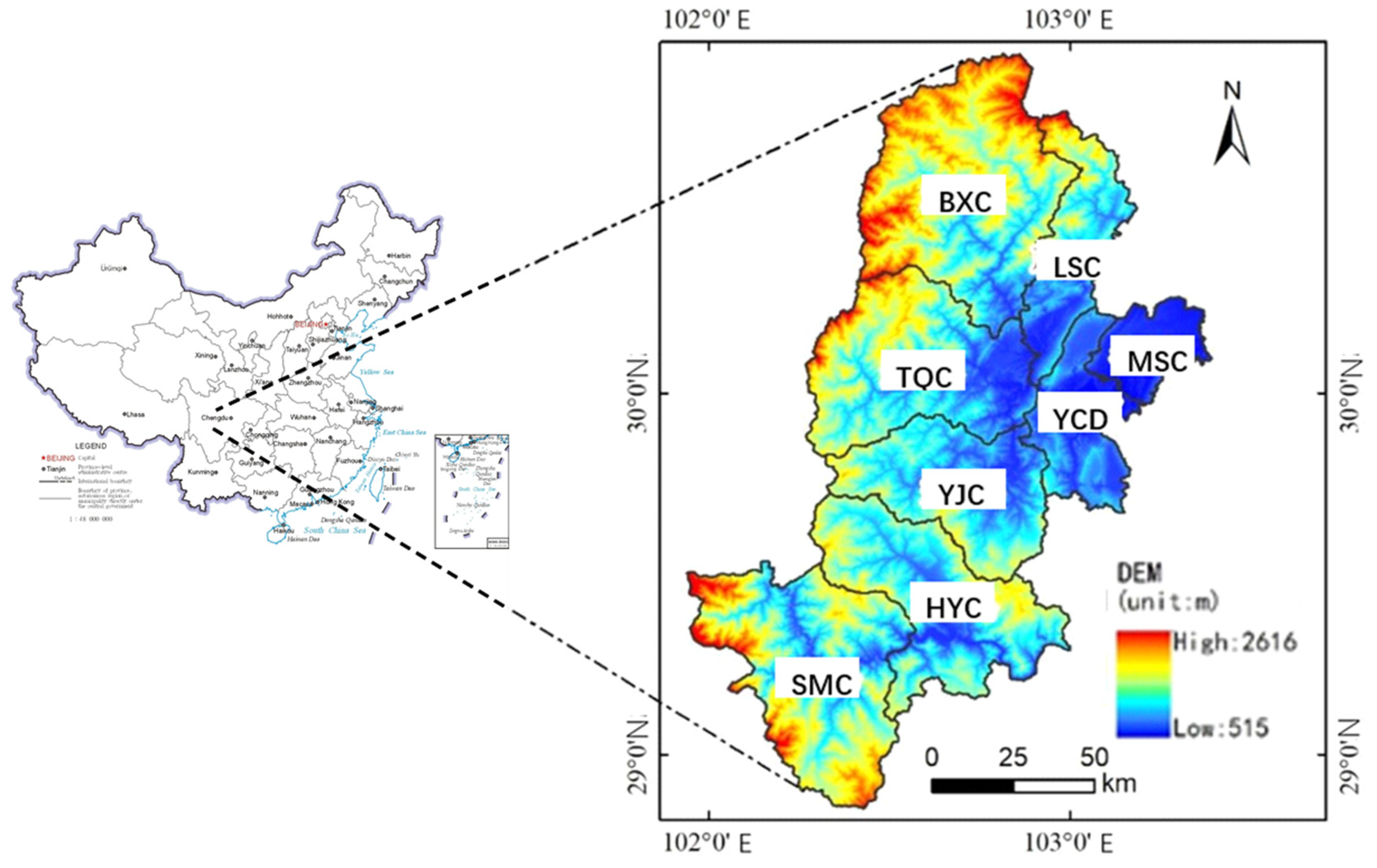
Ya’an City has a total area of 15,046 square kilometers, with two districts and six counties under its jurisdiction (Figure 1 shows the geographic location of the study area. The national approval number for the map is GS(2019)1673): Yucheng District (YCD), Mingshan County (MSC), Yingjing County (YJC), Hanyuan County (HYC), Shimian County (SMC), Tianquan County (TQC), Lushan County (LSC), and Baoxing County (BXC). Ya’an City is a famous historical and cultural city in Sichuan Province, as well as an emerging tourist city. The current difficulties faced by Ya’an City since the implementation of the “rural revitalization” strategy are studied here; at the same time, by measuring the coupling co-scheduling of “PF–LF–EF”, a theoretical exploration is provided for the sustainable development of Ya’an City (http://www.stats.gov.cn/ (accessed on 20 May 2024)).
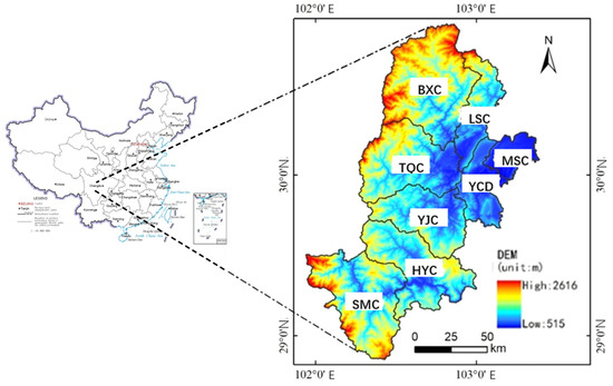
Figure 1.
Study area.
4. Materials and Methods
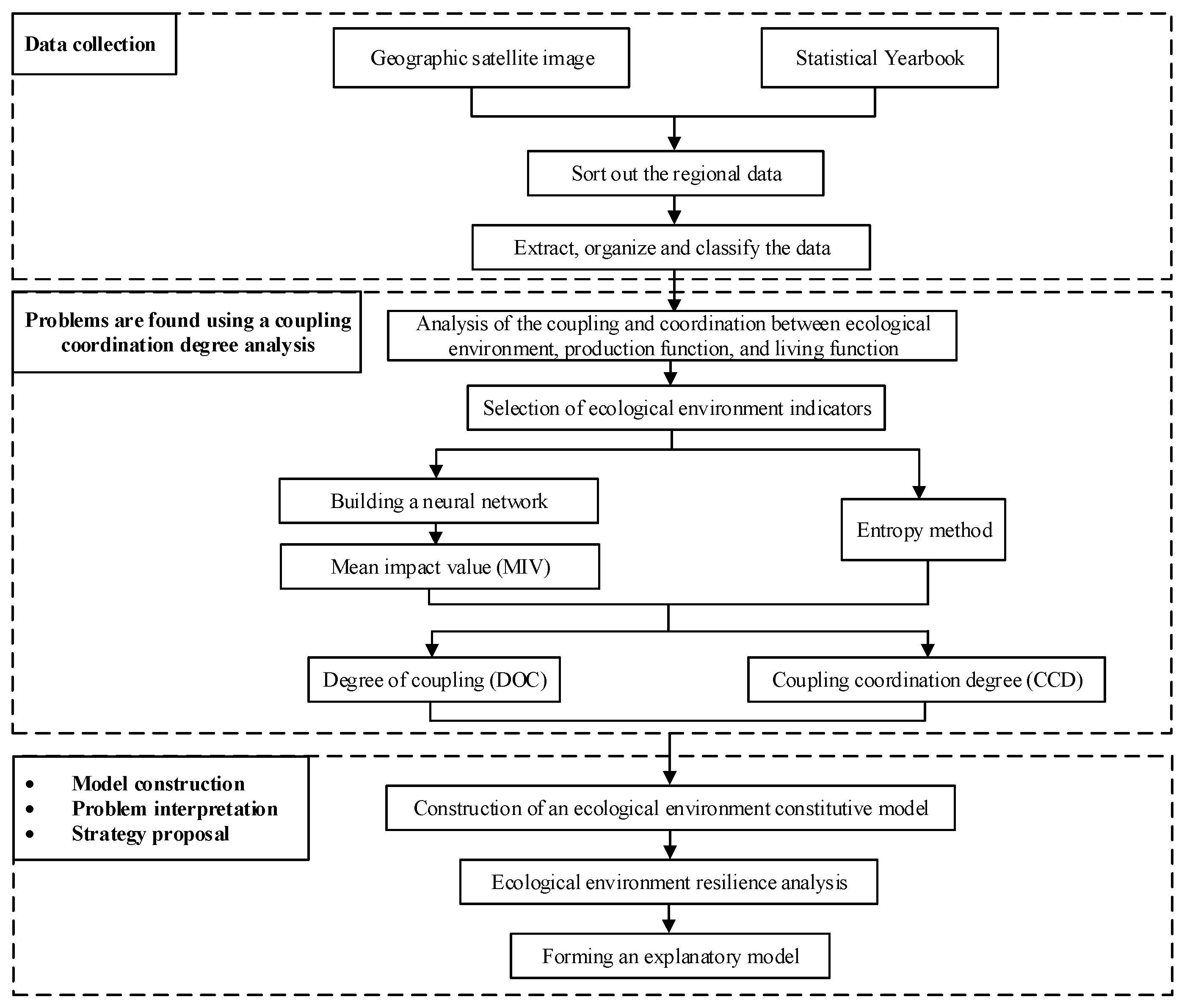
The main methods used in this study include (1) a coupling coordination model, (2) the combination weighting method, and (3) a constitutive model analysis. (Figure 2 shows a technical roadmap of this study).

Figure 2.
Technical roadmap.
4.1. Coupling Coordination Model
The construction of Ya’an City under the premise of rural revitalization is inevitably an organic coupling of production space, living space, and ecological space, and the value can be represented spatially through PF, LF, and EF. The strength of the coupling effect can be determined by calculating the coupling degree for “PF–LF–EF space”, which has practical significance for exploring the renewal of Ya’an City [31]. The specific calculation formula is as follows [32,33,34]:
where C is the coupling degree between the three spatial functions in Ya’an City, with a value range of [0, 1]. The size of C is determined by the evaluation values of the three spatial functions in Ya’an City, and the larger the value, the stronger the interaction and influence between the three spatial functions in Ya’an City. represent the comprehensive evaluation values of PF, LF, and EF in Ya’an City. The coupling degree calculation model uses the following formula:
Based on existing research results and combined with the actual situation in this study, the three spatial functional coupling degrees are divided into four types (see Table 1).

Table 1.
Classification of coupling degree types.
Although the coupling degree can reflect the relationship between the three spatial functions, it cannot characterize whether each function promotes interactions with one another at high levels or restricts each other to low levels. Therefore, this study introduces a coupling coordination coefficient to construct three spatial function coupling coordination models [35]:
where C is the three spatial DOC values; D is the three spatial CCD values; PF, LF, and EF are the evaluation values for production space, living space, and ecological space, respectively; and a, b, and c are the undetermined coefficients of production space, living space, and ecological space, respectively.
According to this formula, the coupling co-scheduling between two of the three spatial functions can be obtained:
where the weights of a, b, and c are not assigned the same value but are determined based on neural network algorithms. Referring to relevant research results, Table 2 divides the coupling coordination degree of the three spatial functions into two major categories and eight subcategories. Additionally, DOC refers to the degree of interaction between the two parties, regardless of their pros and cons; CCD refers to the degree of benign coupling in the interaction, reflecting the quality of coordination and indicating whether various functions promote interactions with one another at high levels or constrains each other to low levels.
Table 2.
Classification of coordination types.
4.2. Combination Weighting Method
To overcome some of the drawbacks of the entropy method, neural network algorithms are also applied to calculate the weight values of various influencing factors. Two weight calculation methods are selected, and the results of each weight calculation method are compared and analyzed for comprehensive consideration. Two main aspects need to be considered: firstly, the calculation results need to be compared and analyzed and then potential patterns need to be identified based on their differences; secondly, the accuracy of the analysis needs to be improved, and the shortcomings of a single weighting method need to be compensated for.
The combination weighting method is thus composed of the entropy method and the MIV algorithm, as shown in Formula (5).
where W is the weight of a factor, the weight coefficient β represents the subjective weighting method, and the weight coefficient (1 − β) represents the objective weighting method. When using the combination weighting method, the weight coefficient needs to be determined comprehensively. In this study, β = 1/3.
4.2.1. Entropy Method
The general principle behind the entropy method [36] is that the smaller the information entropy of an index is, the greater the degree of variation in its index value [37], the more information it will provide, the greater its role in a comprehensive evaluation, and thus, the larger the weight should be [38]; conversely, the greater the information entropy of an index, the smaller the variation in its index value, the smaller the amount of information it provides, the smaller the role it plays in a comprehensive evaluation, and the smaller its weight should be [39,40,41]. Therefore, information entropy can be used to calculate the weight of each indicator and provide a basis for the comprehensive evaluation of multiple indicators.
4.2.2. MIV (Mean Impact Value) Algorithm
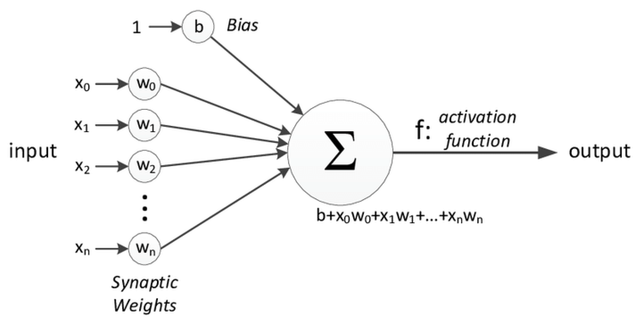
MIV is considered one of the best indicators for evaluating variable weight values in neural networks [42,43]. Therefore, this study is based on the principles of neural network algorithms [44] and combines the various influencing factor indicators selected in that study to construct three neural network algorithm models [45,46], which are BPNN, GMNN, and GRNN, and a constructed neural network [47] is trained to extract complex non-linear patterns in the study area [48,49]. In this study, the MIV algorithm was applied to the trained neural network with the highest accuracy to identify input terms that have a significant impact on the results. Then, a weight analysis was performed using the neural network [50]. To ensure the effectiveness of the simulation results of each neural network, the coefficients of determination (R2) and variation (CV) were calculated and analyzed, and the mean absolute error (MAE) and root mean square error (RMSE) of the three models were calculated separately for comparison and selection of the neural network algorithm with the highest accuracy. Figure 3 shows the topology structure of a single hidden layer feedforward network.
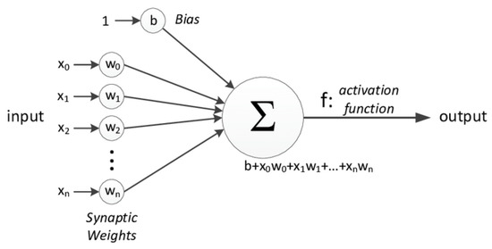
Figure 3.
Single hidden layer neural network topology.
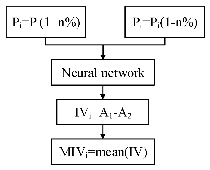
This study selects MIV as the important indicator for evaluating the impact of each independent variable on the dependent variable. MIV is an indicator used to determine the impact of input neurons on output neurons, with symbols representing the direction of correlation and absolute values representing the relative importance of the impact. The specific calculation process is as follows: After the neural network training is terminated, 10% is added or subtracted from the original value of each independent variable feature in training sample P to form two new training samples and . and are used as simulation samples to simulate the built network, and two simulation results and are obtained. The difference between and is the impact value (IV) of changing the independent variable on the output. Finally, the average value is taken and recorded as the MIV value. Figure 4 shows the basic principles of the MIV algorithm.
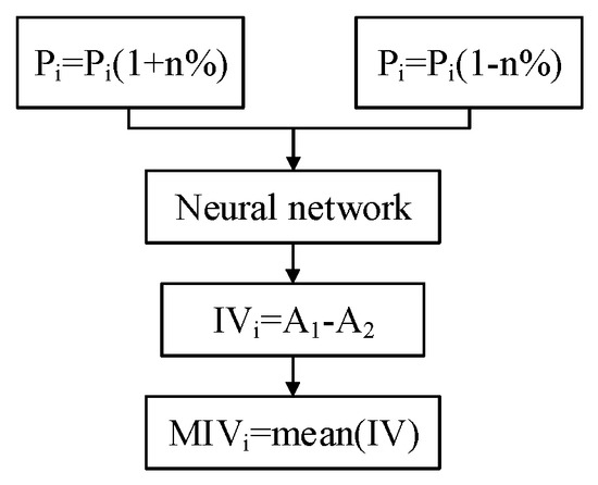
Figure 4.
Basic principles of the MIV algorithm.
4.3. Constitutive Model
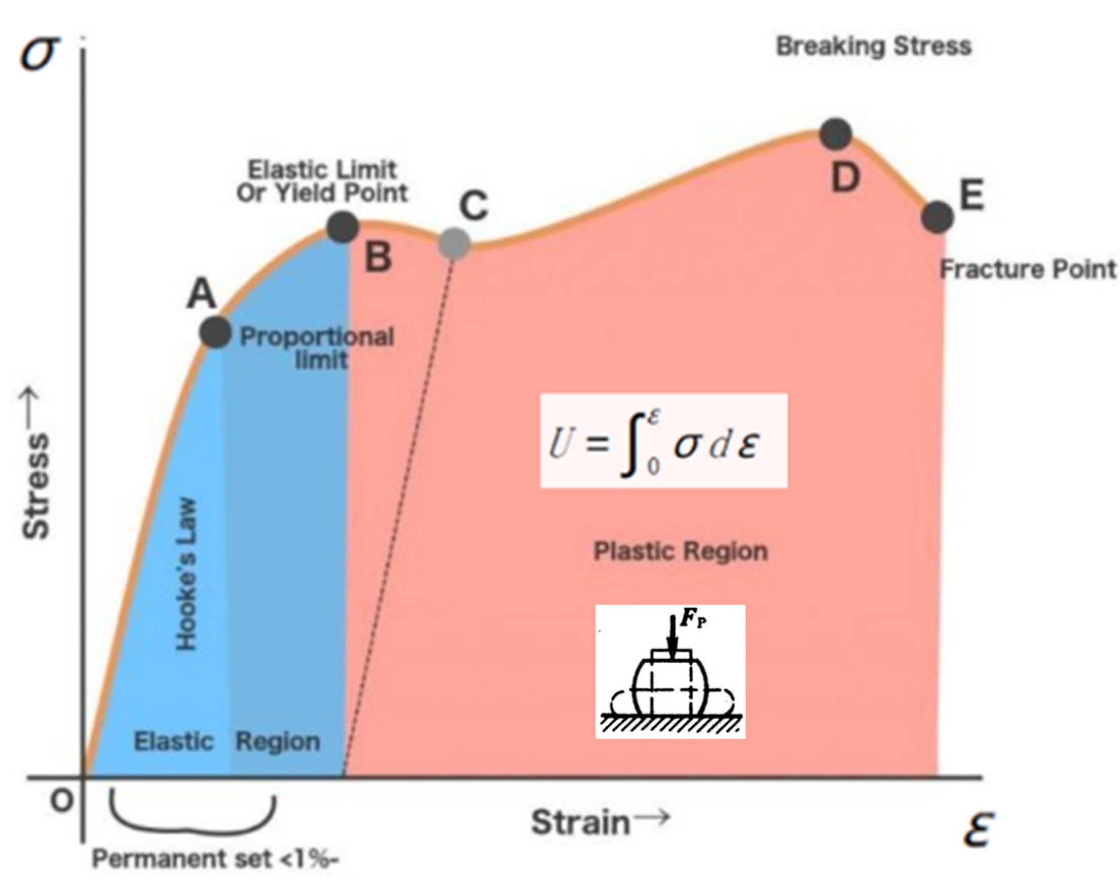
The stress–strain curve corresponding to an object under stress is obtained through tensile or compressive tests. The horizontal axis of the curve is the strain, and the vertical axis is the applied stress. The shape of the curve reflects the various deformation processes that occur in the research object under external forces.
When the stress is below the proportional limit, the stress σ and strain ε are proportional. In the following equation, EF is a constant called the elastic modulus or Young’s modulus, which is the ratio of normal stress to normal strain. The unit of elastic modulus is the same as that of stress. Resilience (U) represents the energy required to deform the research object [51], which is the area enclosed by the stress–strain curve (Figure 5).

Figure 5.
Stress–strain curves of typical materials.
In this study, the above model is applied to analyze the resilience of an ecological space. Human development puts pressure on the ecological and living environment and, when acting on human society, manifests as a reduction in ecological space and an expansion of production and living spaces. To draw the stress–strain curve, the GDP value is selected as the stress value, construction land is selected as a representative of production space and living space, forests and grasslands are selected to represent the EF and changes in the area are analyzed to ultimately draw the images.
5. Results and Analysis
5.1. The Weight Calculation Results of the MIV Algorithm and the Entropy Method
According to the principles of the BPNN algorithm, combined with empirical formulas and trial and error methods, the number of hidden layers of the neural network was determined. Three network models with structures of 14-3-1, 14-4-1, and 14-9-1 were constructed based on different hidden layer numbers; a BPNN with a structure of 1-15-1 was constructed, and a GRNN with a structure of 14-13-2-1 was constructed. This study focuses on the relationship between changes in construction land area and other influencing factors in Ya’an City. Therefore, each neural network was run 1000 times; the evaluation indicators calculated based on the predicted results are shown in Table 3.
Table 3.
A neural network algorithm was used to predict the CLA results of Ya’an City in 2018 (unit: hectare) and analysis indexes.
Then, the BPNN (4HL) with the highest accuracy and stability was selected, the MIV algorithm was added to the algorithm, the MIV algorithm program was run 100 times continuously, the absolute values of the weight values of each influencing factor were recorded, the average of the 100 calculation results was calculated, and the 20 factors were normalized. The results of the 100 runs are presented in an attached table. Table 4 shows the weight values of each influencing factor obtained using the MIV and entropy methods.
Table 4.
Weight values of various indicators in Ya’an City.
5.2. Calculation Results and Analysis of the Coupling Coordination Model
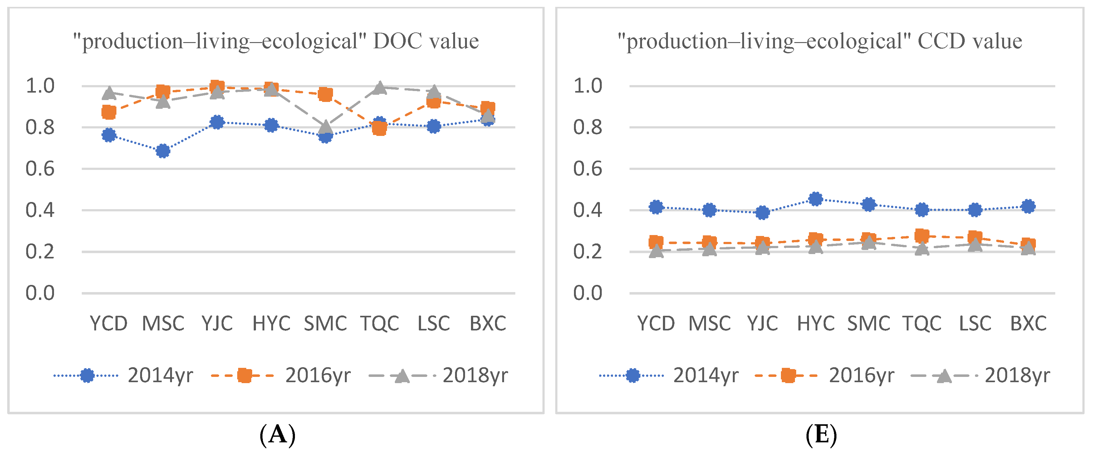
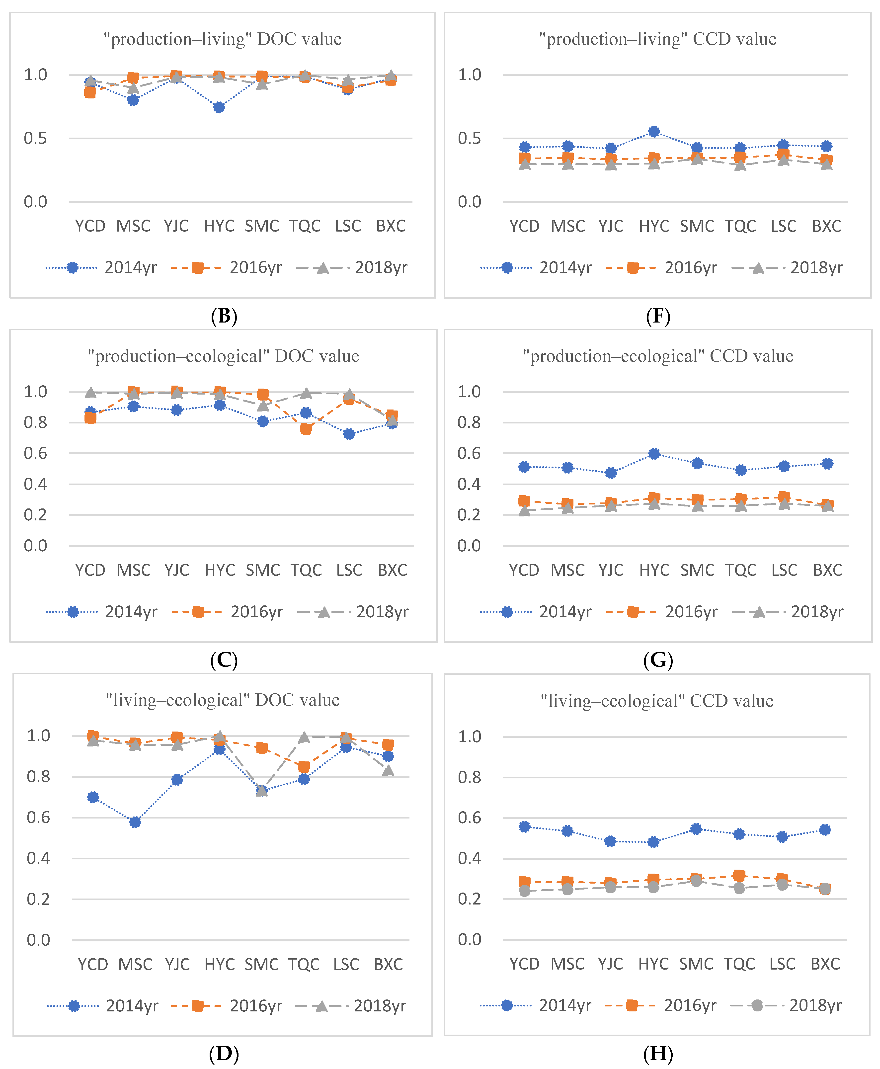
CCD and DOC values were then calculated for eight districts and counties in Ya’an City. Figure 6A–D represent the DOC values between “PF–LF–EF space”, “PF–LF space”, “PF–EF space”, and “LF–EF space”; in Figure 6E–H are the CCD values between “PF–LF–EF space”, “PF–LF space”, “PF–EF space”, and “LF–EF space”. Figure 7 shows the CCD and DOC values reflected in space.
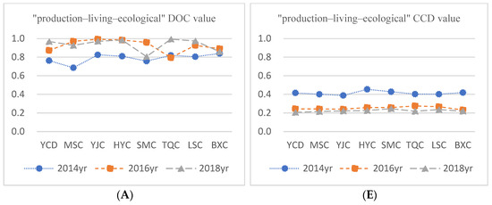
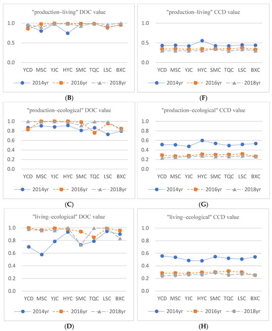
Figure 6.
DOC and CCD values of districts and counties in Ya’an City. Note: The horizontal coordinate in the figure represents the eight counties of Ya’an—Yucheng District (YCD), Mingshan County (MSC), Yingjing County (YJC), Hanyuan County (HYC), Shimian County (SMC), Tianquan County (TQC), Lushan County (LSC), and Baoxing County (BXC). The coupling values for different regions but the same period are connected for easier reading and have no actual meaning.
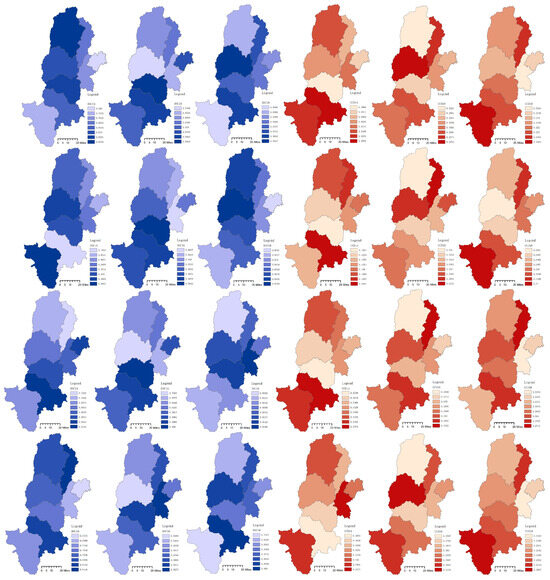
Figure 7.
CCD distribution for eight districts and counties of Ya’an City. Note: This figure has four rows and six columns, resulting in 24 images. Rows sequentially represent the “production–living–ecological space”, “production–living space”, “production–ecological space”, and “living–ecological space” of Ya’an City. Columns represent the DOC and CCD values, with the first three representing the spatial reflection of DOC values for 2014, 2016, and 2018 and the last three representing the spatial reflection of CCD values for 2014, 2016, and 2018.
The analysis results indicate that the overall spatial coupling of various districts and counties in Ya’an City is relatively high, with the coupling degree of “PF–LF–EF space” divided into four stages: low coupling, antagonism, run-in, and high coupling. Most of the different spatial coupling values calculated based on the three time periods in this study are in the range of 0.8 to 1.0. According to the calculation results, during the development of Ya’an City, all districts and counties were in an imbalanced coupling state and have since reached extreme or severe imbalance, indicating that all counties and districts in Ya’an City have not transited from high coupling to high coordination. With the development of Ya’an City, the coupling and coordination values of various districts and counties have significantly decreased for two main reasons: Firstly, the ecological protection policies implemented by Ya’an City have made the “ecological space” significantly more important than “production–living space”. Secondly, with the advancement of urbanization in Ya’an City, the “production space” has increasingly become more severely caught between the “living space” and the “ecological space”, leading to a gradual decrease in the coupling and coordination between different functional spaces at any time.
Due to the high-level interaction between the “PF–LF–EF spaces” in various districts and counties of Ya’an City, the DOC values are high. The analysis results show that the CCD values of the eight districts and counties in Ya’an City have all decreased, especially the CCD values for “PF–EF space” and “LF–EF space”, while the CCD values of “LF–PF space” have not changed significantly, indicating a natural interdependence between “LF–PF spaces”, with the results also indicating that “PF–EF spaces” and “LF–EF spaces” have difficulty in obtaining a balance. We also constructed an explanatory model based on transmission theory in a following study. We attempted to provide model-based solutions and planning suggestions for how to efficiently utilize the “PF–LF–EF space”.
5.3. Ecological Environment Constitutive Model of Ya’an City
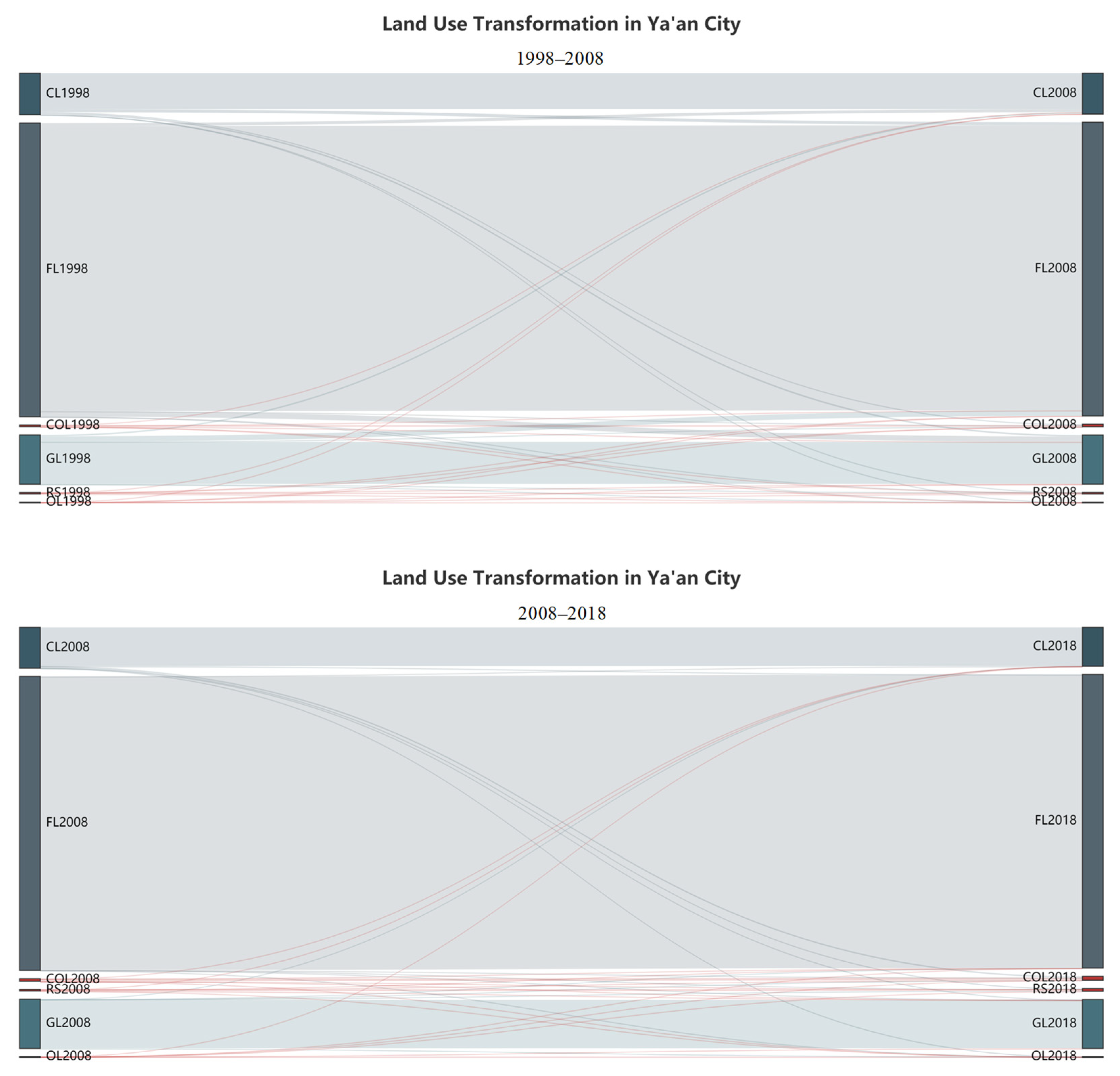
The constitutive model requires values of stress and strain. In this study, GDP value was selected as the stress value, construction land was selected to represent the production space and living space, woodlands and grasslands were selected to represent EF, and the change in area was analyzed to draw the images. Figure 8 is a Sankey map drawn according to the land transfer matrix.
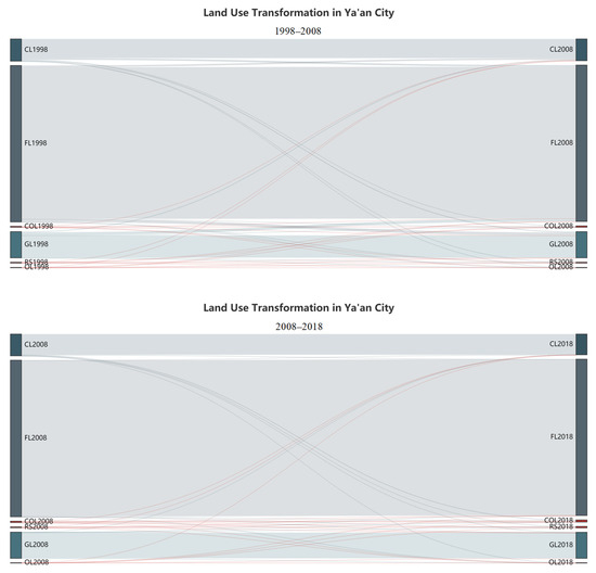
Figure 8.
Changes in land use scale in Ya’an City from 1998 to 2008 and from 2008 to 2018. Note: The abbreviations for the various land use types are as follows: CL (cultivated land), FL (forest land), GL (grassland), RS (river surface), COL (construction land), and OL (other land).
In human settlements, various human activities will exert pressure on EF. Therefore, the “energy” absorbed by EF can be calculated by studying the scale change for EF under the action of human beings. This value also represents the resilience of EF. The horizontal coordinate of the curve shows the strain on EF, and the vertical coordinate shows the pressure on EF from human activities, production spaces, and living spaces. With these scale changes, stiffness degradation and resilience change in the EF in Ya’an City under human activities can be analyzed based on this curve.
As introduced above, in this study, constitutive models are constructed, with the ecological space representing the EF of Ya’an City and the production space and living space representing human activities. Resilience represents the ability of an object of study to absorb energy during plastic deformation and fracture. The better the resilience, the lower the possibility of brittle fracture. Resilience refers to the resistance of an object to fracture when subjected to a force that causes it to deform and is defined as the area of the stress–strain curve.
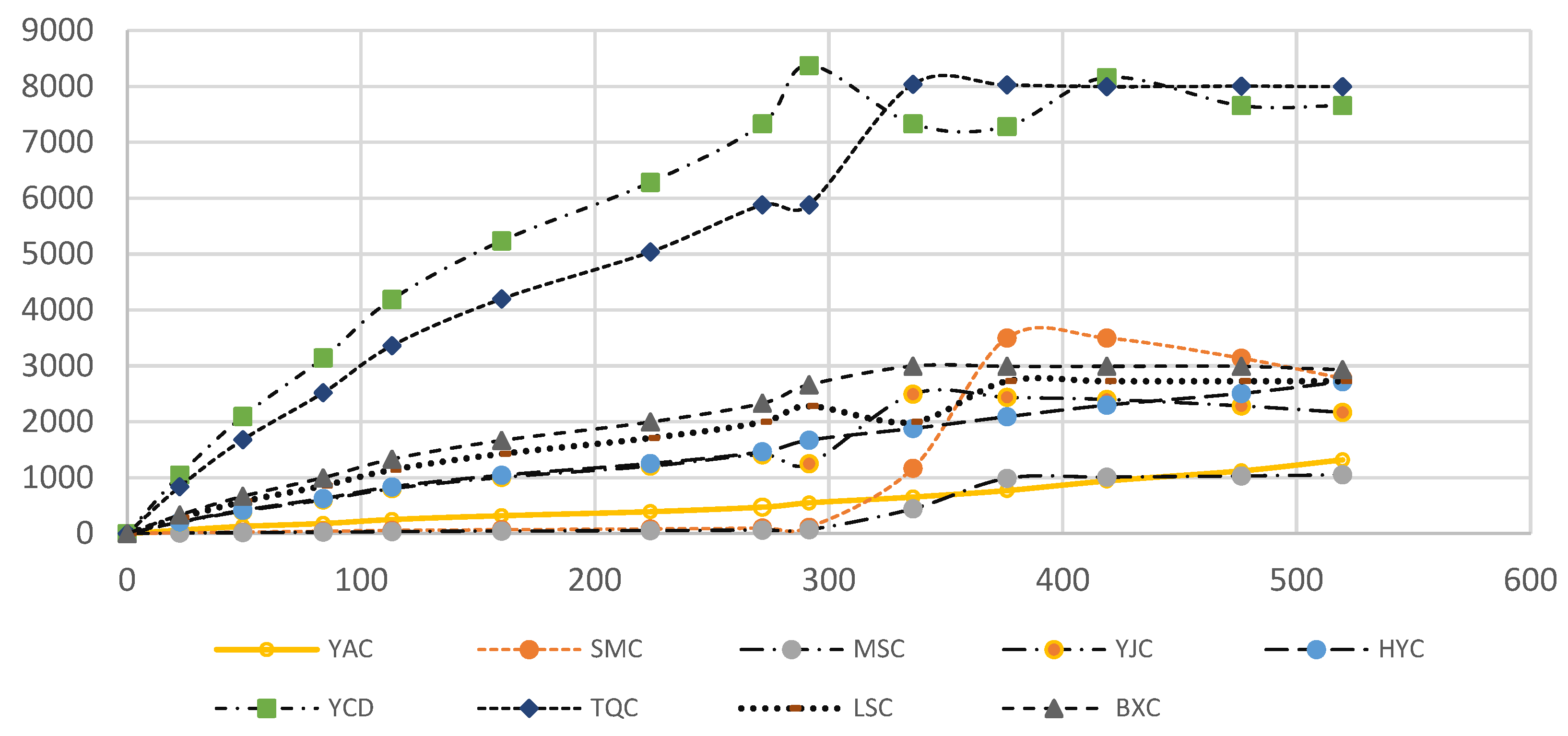
The meaning of this stress–strain curve has been described earlier. The curve represents the changes in land use scale caused by human activities in various regions, and the area enclosed by the curve and the horizontal axis represents the amount of energy absorbed by the “EF–PF–LF space”. For the convenience of calculation, based on the stress–strain values of each region, the stress–strain maps of each region are roughly fitted. The fitting result is shown in Figure 9, with the equations for each curve shown in Table 5. Of note, the purpose of the fitting is to facilitate the calculation of the area enclosed by the curve and the horizontal axis and to conduct a quantitative comparative analysis of each region on a numerical scale.

Figure 9.
Ecological environment constitutive model of districts and counties in Ya’an City. Note: The only solid line in the figure represents the resilience constitutive model of production and living functions in Ya’an City. The remaining eight dashed lines represent the ecological environment resilience curves of the eight districts and counties in Ya’an City.
Table 5.
The stress–strain fitting values of EF in each region.
According to the results of the figure above, the fitting of each curve was carried out, and the integral was used to calculate the area of each district and county, representing the resilience of each district and county in Ya’an City, respectively. The calculation results are as follows:
The research results indicate that, in the field of EF, strain amplitude increases with increasing stress, and the “stiffness” of EF decreases with increasing stress, similar to the behavior of typical metals in material mechanics.
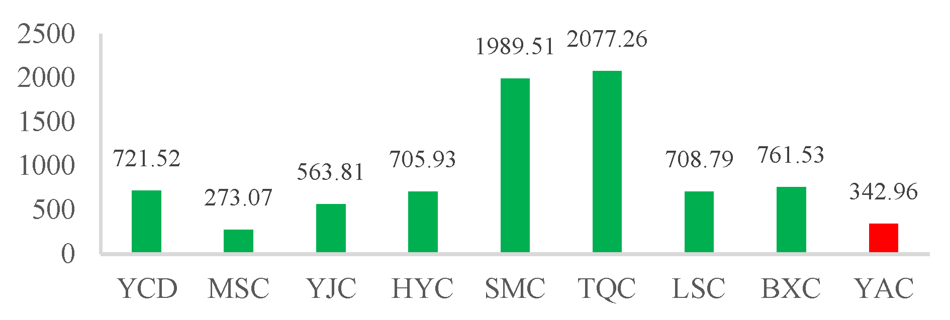
Through the analysis of resilience values, the area enclosed by the constitutive model of PF and LF in Ya’an City represents its resilience, and the calculated result is 342.96 kJ. The area enclosed by the EF constitutive model curve and coordinate axis of each district and county in Ya’an City represents the resilience of EF. The calculation results of each district and county are shown in Table 6.
Table 6.
Calculated values of resilience in each zone.
The resilience value in this study also characterizes the amount of “energy” that this function absorbs from the pressure caused by human beings on the natural environment. Under the same stress conditions, the resilience values of the EF in each district of Ya’an City are much greater than the resilience values of PF and LF. This indicates that during the development of Ya’an City, EF absorbed a large amount of human stress, which explains the low coordination between the ecological space, production space, and living space in Ya’an City. The pressure caused by human activities has been heavily transferred to EF, resulting in an imbalance between EF, PF, and LF. The calculation results of each district and county are shown in Figure 10.
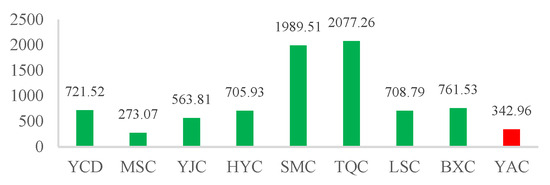
Figure 10.
Resilience values of the ecological environment in different regions.
6. Conclusions and Discussion
In the past few decades, China has witnessed rapid development, particularly in terms of its economy and urbanization. However, during development, the coordinated development of EF, PF, and LF in the living environment is often overlooked. Here, we took Ya’an City in China as a research case and discovered an imbalanced development between EF, PF, and LF, with the greatest decrease in coordination between EF and the other two types of functions. Next, a constitutive model was constructed to quantify the resilience of EF, PF, and LF in Ya’an City. The calculation results showed that the resilience values of EF in various regions of Ya’an were much greater than the sum of the resilience values of PF and LF. This indicates that, during economic development, the EFs of various regions in Ya’an City bear the “pressure” generated by the development, which explains the reason for the significant decrease in coordination between EF and the other two types of functions.
In this study, we optimized the method of calculating the DOC and COD. Then we proposed a theoretical model to analyze the ecological functions bearing the pressure of human activities from qualitative and quantitative perspectives. The research results can provide an analytical framework, path, and method for the coordinated development of ecological, production, and living functions in other regions. We also developed a repeatable technological pathway for discovering EF, PF, and LF while providing precise guidance and suggestions for governments and relevant decision-makers to solve problems. Firstly, within the development process, more attention should be paid to the DOC and CCD development of EF, PF, and LF, and key functional issues in different research areas should be identified. Secondly, a resilience analysis and an evaluation of the EF, PF, and LF of the research area should be conducted before decisions are made, and based on this analysis, subsequent development strategies should be formulated. Finally, by constructing a constitutive model of the research area, the resilience values of various functions can be analyzed to identify prominent issues in the development of the research area.
Some shortcomings of this study also need to be noted: (1) Poor interpretability of neural networks has always been a problem in the academic field [52]. Here, we tried to use an MIV algorithm to explain the results, but some research conclusions have still not fully explained. (2) The constitutive model analysis in this paper is also a little rough, and a more detailed quantitative analysis is needed in the future [53]. Possible future research directions include (1) a further subdivision of the specific meanings of EF, PF, and LF studied in this paper, which requires more data support, and (2) a thorough study of the constitutive model mechanism in this article, an analysis of interventions, and the determination of the desired constitutive model curve to achieve the maximum benefits.
Author Contributions
Methodology, Y.Z.; Validation, Y.Z.; Resources, W.L.; Data curation, W.L.; Writing—original draft, W.L.; Supervision, Y.H.; Project administration, Y.H.; Funding acquisition, Y.H. All authors have read and agreed to the published version of the manuscript.
Funding
The work is funded by the Chongqing Natural Science Foundation General Project (CSTB2023NSCQ-MSX1003).
Institutional Review Board Statement
Not applicable.
Informed Consent Statement
Not applicable.
Data Availability Statement
The data and code will be made available on reasonable request.
Conflicts of Interest
There is no conflict of interest associated with this research work.
References
- Liu, J.; Yang, C.; Yin, T.; Wang, Z.; Qu, S.; Suo, Z. Polyacrylamide hydrogels. II. Elastic dissipater. J. Mech. Phys. Solids 2019, 133, 103737. [Google Scholar] [CrossRef]
- Gomez Limón, J.A.; Arriaza, M. What does society demand from rural areas? Evidence from Southern Spain. New Medit Mediterr. J. Econ. Agric. Environ. 2013, 12, 2–12. [Google Scholar]
- Ma, W.; Jiang, G.; Li, W.; Zhou, T.; Zhang, R. Multifunctionality assessment of the land use system in rural residential areas: Confronting land use supply with rural sustainability demand. J. Environ. Manag. 2019, 231, 73–85. [Google Scholar] [CrossRef] [PubMed]
- You, H.; Zhang, X. Sustainable livelihoods and rural sustainability in China: Ecologically secure, economically efficient or socially equitable? Resour. Conserv. Recycl. 2017, 120, 1–13. [Google Scholar] [CrossRef]
- Liu, Y.S. Rural transformation development and new countryside construction in eastern coastal area of China. Acta Geogr. Sin. 2007, 62, 563–570. [Google Scholar]
- Tu, S.S.; Long, H.L.; Li, T.T. The mechanism and models of villages and towns construction and rural development in China. Econ. Geogr. 2015, 35, 141–160. [Google Scholar]
- Fang, Y.G.; Liu, J.S. Diversified agriculture and rural development in China based on multifunction theory: Beyond modernization paradigm. Acta Geogr. Sin. 2015, 70, 257–270. [Google Scholar]
- Long, H.L.; Tu, S.S.; Ge, D.Z.; Li, T.T.; Liu, Y.S. The allocation and management of critical resources in rural China under restructuring: Problems and prospects. J. Rural Stud. 2016, 47, 392–412. [Google Scholar] [CrossRef]
- Liao, G.T.; He, P.; Gao, X.S.; Deng, L.J.; Zhang, H.; Feng, N.N.; Zhou, W.; Deng, O.P. The Production-Living-Ecological Land Classification System and Its Characteristics in the Hilly Area of Sichuan Province, Southwest China Based on Identification of the Main Functions. Sustainability 2019, 11, 1600. [Google Scholar] [CrossRef]
- Huang, J.C.; Lin, H.X.; Qi, X.X. A literature review on optimization of spatial development pattern based on ecological-production-living space. Progr. Geograp. 2017, 36, 378–391. [Google Scholar]
- Chan, P. Child-Friendly Urban Development: Smile Village Community Development Initiative in Phnom Penh. World 2021, 2, 505–520. [Google Scholar] [CrossRef]
- Ao, P.N. COVID, CITIES and CLIMATE: Historical Precedents and Potential Transitions for the New Economy. Urban Sci. 2020, 4, 32. [Google Scholar] [CrossRef]
- Hao, H.M.; Ren, Z.Y. Land Use/Land Cover Change (LUCC) and Eco-Environment Response to LUCC in Farming-Pastoral Zone, China. Agric. Sci. China 2009, 8, 91–97. [Google Scholar] [CrossRef]
- Minh, H.V.T.; Avtar, R.; Mohan, G.; Misra, P.; Kurasaki, M. Monitoring and Mapping of Rice Cropping Pattern in Flooding Area in the Vietnamese Mekong Delta Using Sentinel-1A Data: A Case of An Giang Province. ISPRS Int. J. Geo-Inf. 2019, 8, 211. [Google Scholar] [CrossRef]
- Veettil, B.K.; Quang, N.X.; Trang, N.T.T. Changes in mangrove vegetation, aquaculture and paddy cultivation in the Mekong Delta: A study from Ben Tre Province, southern Vietnam. Estuar. Coast. Shelf Sci. 2019, 226, 106273. [Google Scholar] [CrossRef]
- Yu, J.; Zhou, K.; Yang, S. Land use efficiency and influencing factors of urban agglomerations in China. Land Use Policy 2019, 88, 104143. [Google Scholar] [CrossRef]
- Tran, H.; Tran, T.; Kervyn, M. Dynamics of Land Cover/Land Use Changes in the Mekong Delta, 1973–2011: A Remote Sensing Analysis of the Tran Van Thoi District, Ca Mau Province, Vietnam. Remote Sens. 2015, 7, 2899–2925. [Google Scholar] [CrossRef]
- Zhang, X.; Xu, Z. Functional Coupling Degree and Human Activity Intensity of Production–Living–Ecological Space in Underdeveloped Regions in China: Case Study of Guizhou Province. Land 2021, 10, 56. [Google Scholar] [CrossRef]
- Allam, Z.; Bibri, S.E.; Chabaud, D.; Moreno, C. The ‘15-Minute City’ concept can shape a net-zero urban future. Humanit. Soc. Sci. Commun. 2022, 9, 126. [Google Scholar] [CrossRef]
- Moreno, C.; Allam, Z.; Chabaud, D.; Gall, C.; Pratlong, F. Introducing the “15- Minute City”: Sustainability, resilience and place identity in future post-pandemic cities. Smart Cities 2021, 4, 93–111. [Google Scholar] [CrossRef]
- Mittal, S.; Chadchan, J.; Mishra, S.K. Review of concepts, tools and indices for the assessment of urban quality of life. Soc. Indic. Res. 2020, 149, 187–214. [Google Scholar] [CrossRef]
- Liu, D.Y.; Zheng, X.Q.; Zhang, C.X.; Wang, H.B. A new temporal–spatial dynamics method of simulating land-use change. Ecol. Model. 2017, 350, 1–10. [Google Scholar] [CrossRef]
- Phiri, D.; Morgenroth, J.; Xu, C. Long-term land cover change in Zambia: An assessment of driving factors. Sci. Total Environ. 2019, 697, 134206. [Google Scholar] [CrossRef] [PubMed]
- Arabameri, A.; Saha, S.; Roy, J.; Tiefenbacher, J.P.; Cerda, A.; Biggs, T.; Pradhan, B.; Ngo, P.T.T.; Collins, A.L. A novel ensemble computational intelligence approach for the spatial prediction of land subsidence susceptibility. Sci. Total Environ. 2020, 726, 138595. [Google Scholar] [CrossRef] [PubMed]
- Li, H.-Z.; Tao, W.; Gao, T.; Li, H.; Lv, Y.-H.; Su, Z.-M. Improving the Accuracy of DFT Calculation for Homolysis Bond Dissociation Energies of Y-NO Bond via Back Propagation Neural Network Based on Mean Impact Value. Chem. J. Chin. Univ. Chin. 2012, 33, 346–352. [Google Scholar]
- Park, S.; Choi, C.; Kim, B.; Kim, J. Landslide susceptibility mapping using frequency ratio, analytic hierarchy process, logistic regression, and artificial neural network methods at the Inje area, Korea. Environ. Earth Sci. 2013, 68, 1443–1464. [Google Scholar] [CrossRef]
- Xing, L.; Xue, M.G.; Hu, M.S. Dynamic simulation and assessment of the coupling coordination degree of the economy–resource–environment system: Case of Wuhan City in China. J. Environ. Manag. 2019, 230, 474–487. [Google Scholar] [CrossRef] [PubMed]
- Willemen, L.; Hein, L.; van Mensvoort, M.E.; Verburg, P.H. Space for people, plants, and livestock? Quantifying interactions among multiple landscape functions in a Dutch rural region. Ecol. Ind. 2010, 10, 62–73. [Google Scholar] [CrossRef]
- Zheng, X.Y.; Liu, Y.S. Connotation, formation mechanism and regulation strategies of rural disease in the new epoch in China. Hum. Geogr. 2018, 33, 100–106. [Google Scholar]
- Liu, Y.S.; Zhou, Y.; Li, Y.H. Rural regional system and rural revitalization strategy in China. Acta Geogr. Sin. 2019, 74, 2511–2528. [Google Scholar]
- Wang, J.Y.; Wang, S.J.; Li, S.J.; Feng, K.S. Coupling analysis of urbanization and energy-environment efficiency: Evidence from Guangdong province. Appl. Energy 2019, 254, 113650. [Google Scholar] [CrossRef]
- Bellin, A.; Majone, B.; Cainelli, O.; Alberici, D.; Villa, F. A continuous coupled hydrological and water resources management model. Environ. Modell. Softw. 2016, 75, 176–192. [Google Scholar] [CrossRef]
- Song, Z.Y.; Frühwirt, T.; Konietzky, H. Inhomogeneous mechanical behavior of concrete subjected to monotonic and cyclic loading. Int. J. Fatig. 2020, 132, 105383. [Google Scholar] [CrossRef]
- Zhou, D.; Xu, J.C.; Lin, Z.L. Conflict or coordination? Assessing land use multi functionalization using production-living-ecology analysis. Sci. Total Environ. 2017, 577, 136–147. [Google Scholar] [CrossRef] [PubMed]
- Wang, C.; Tang, N. Spatio-temporal characteristics and evolution of rural pro duction-living-ecological space function coupling coordination in Chongqing Municipality. Geograph. Res. 2018, 6, 1100–1114. [Google Scholar]
- Shemshadi, A.; Shirazi, H.; Toreihi, M.; Tarokh, M.J. A fuzzy VIKOR method for supplier selection based on entropy measure for objective weighting. Expert Syst. Appl. 2011, 38, 12160–12167. [Google Scholar] [CrossRef]
- Tang, Z. An integrated approach to evaluating the coupling coordination between tourism and the environment. Tour. Manag. 2015, 46, 11–19. [Google Scholar] [CrossRef]
- Zou, Z.H.; Yun, Y.; Sun, J.N. Entropy method for determination of weight of evaluating in fuzzy synthetic evaluation for water quality assessment indicators. J. Environ. Sci. 2006, 18, 1020–1023. [Google Scholar] [CrossRef]
- He, J.; Wang, S.; Liu, Y.; Ma, H.; Liu, Q. Examining the relationship between urbanization and the eco-environment using a coupling analysis: Case study of Shanghai, China. Ecol. Ind. 2017, 77, 185–193. [Google Scholar] [CrossRef]
- Li, W.; Yi, P. Assessment of city sustainability—Coupling coordinated development among economy, society and environment. J. Clean. Prod. 2020, 256, 120453. [Google Scholar] [CrossRef]
- Wang, Q.S.; Yuan, X.L.; Cheng, X.X.; Mu, R.M.; Zuo, J. Coordinated development of energy, economy and environment subsystems-A case study. Ecol. Ind. 2014, 46, 514–523. [Google Scholar] [CrossRef]
- Gardner, M.W.; Dorling, S.R. Artificial neural networks (the multilayer perceptron)—A review of applications in the atmospheric sciences. Atmos. Environ. 1998, 32, 2627–2636. [Google Scholar] [CrossRef]
- Haykin, S.S. Neural Networks and Learning Machines; Pearson Education: Upper Saddle River, NJ, USA, 2009; Volume 3. [Google Scholar]
- Chen, T. Fitting an uncertain productivity learning process using an artificial neural network approach. Comput. Math. Organ. Theory 2018, 24, 422–439. [Google Scholar] [CrossRef]
- Pham, B.T.; Bui, D.T.; Prakash, I.; Dholakia, M.B. Hybrid integration of Multilayer Perceptron Neural Networks and machine learning ensembles for landslide susceptibility assessment at Himalayan area (India) using GIS. Catena 2017, 149, 52–63. [Google Scholar] [CrossRef]
- Tien Bui, D.; Tuan, T.A.; Klempe, H.; Pradhan, B.; Revhaug, I. Spatial prediction models for shallow landslide hazards: A comparative assessment of the efficacy of support vector machines, artificial neural networks, kernel logistic regression, and logistic model tree. Landslides 2015, 13, 361–378. [Google Scholar] [CrossRef]
- Xie, L.; Wei, R.; Hou, Y. Ship Equipment Fault Grade Assessment Model Based on Back Propagation Neural Network and Genetic Algorithm. In Proceedings of the 2008 International Conference on Management Science & Engineering, Long Beach, CA, USA, 10–12 September 2008; pp. 211–218. [Google Scholar]
- Lin, J.-W.; Chao, C.-T.; Chiou, J.-S. Determining Neuronal Number in Each Hidden Layer Using Earthquake Catalogues as Training Data in Training an Embedded Back Propagation Neural Network for Predicting Earthquake Magnitude. IEEE Access 2018, 6, 52582–52597. [Google Scholar] [CrossRef]
- Wang, L.; Zeng, Y.; Chen, T. Back propagation neural network with adaptive differential evolution algorithm for time series forecasting. Expert Syst. Appl. 2015, 42, 855–863. [Google Scholar] [CrossRef]
- Ren, C.; An, N.; Wang, J.; Li, L.; Hu, B.; Shang, D. Optimal parameters selection for BP neural network based on pstudy swarm optimization: A case study of wind speed forecasting. Knowl.-Based Syst. 2014, 56, 226–239. [Google Scholar] [CrossRef]
- Li, Y.; Li, Y.; Zhou, Y.; Shi, Y.; Zhu, X. Investigation of a coupling model of coordination between urbanization and the environment. J. Environ. Manag. 2012, 98, 127–133. [Google Scholar] [CrossRef] [PubMed]
- Halgamuge, S. FAIR AI: A Conceptual Framework for Democratisation of 21st Century AI. In Proceedings of the International Conference on Instrumentation, Control, and Automation (ICA), Bandung, Indonesia, 25–27 August 2021; pp. 1–3. [Google Scholar]
- Cao, X.; Liu, M. The dynamic evolution of resource and environment carrying capacity responsing to urbanization in China and Russia from the perspective of human land relationship. World Agric. 2018, 202–208. [Google Scholar]

Disclaimer/Publisher’s Note: The statements, opinions and data contained in all publications are solely those of the individual author(s) and contributor(s) and not of MDPI and/or the editor(s). MDPI and/or the editor(s) disclaim responsibility for any injury to people or property resulting from any ideas, methods, instructions or products referred to in the content. |
© 2024 by the authors. Licensee MDPI, Basel, Switzerland. This article is an open access article distributed under the terms and conditions of the Creative Commons Attribution (CC BY) license (https://creativecommons.org/licenses/by/4.0/).