Environmental, Geographical, and Economic Impacts of Inbound Tourism in China: A Mixed-Effects Gravity Model Approach

Abstract

This study examines the dynamics of inbound tourism in China, utilizing a mixed-effects gravity model to analyze data from urban clusters around China’s three major airports. The research methodology of the study includes applying advanced econometric techniques, such as the Poisson pseudo-maximum likelihood estimation, to ensure robust and accurate results. The study focuses on international tourist arrivals and foreign exchange earnings, identifying key drivers such as tourism resources, transportation safety, and service quality. Our findings indicate a 10% increase in per capita GDP correlates with a 0.88% rise in inbound tourist numbers. Additionally, proximity to major urban centers like Beijing, Shanghai, and Guangzhou significantly influences tourist arrivals, with every 100 km increase in distance resulting in a 5.56% decrease in tourist numbers. The study also explores the impact of environmental factors on tourism, suggesting that improvements in green coverage and reductions in industrial waste and traffic fatalities could enhance tourist arrivals. Conversely, environmental protection measures can both positively and negatively impact tourism. This research provides a strategic blueprint for policymakers and professionals in tourism and environmental sustainability, emphasizing the importance of integrated environmental sustainability in tourism development strategies. The model accounts for up to 79% of the variability in inbound tourism flows, offering robust evidence that economic and policy dimensions impact tourism.

1. Introduction

In the context of escalating globalization and expanding international trade, tourism has emerged as a significant economic stimulant, profoundly impacting global economies. Particularly, inbound tourism acts as a catalyst for cultural exchange and economic enhancement in host countries. The volume of inbound tourists and corresponding foreign exchange income serve as critical indicators of a destination’s tourism development status and its integration into the global economic landscape [1]. This study examines the dynamics of inbound tourism in China, employing a mixed-effects gravity model to analyze data from urban clusters around the three major airports in Beijing, Shanghai, and Guangzhou. The research identifies the key drivers influencing international tourist arrivals and foreign exchange earnings, offering strategic insights for policymakers and professionals in tourism and environmental sustainability.

Despite extensive research, a significant gap persists in the literature in understanding how environmental sustainability intersects with economic factors to shape the future of tourism in China’s rapidly urbanizing regions. Previous studies have often neglected the comprehensive integration of economic and environmental dimensions in analyzing tourism flows. This study addresses the primary question: how do economic, geographical, and environmental factors influence inbound tourism in China? More specifically, it explores how enhancements in green coverage, reductions in industrial waste, and improvements in traffic safety impact tourist arrivals, alongside the potential positive and negative effects of environmental protection measures on tourism.

The focus of this research is on external tourist flows, particularly examining the roles of Beijing, Shanghai, and Guangzhou as major international gateways. These cities, home to some of the world’s busiest airports, handle a substantial portion of the international air traffic entering China. The study aims to provide a sophisticated understanding of how international tourism influences regional development strategies and economic policies, concentrating specifically on external flows. This focus is vital for a comprehensive analysis of global tourism dynamics, economic impacts, and the strategic planning essential for sustainable tourism development in these key urban centers.

Grounded in the theoretical framework of the gravity model of international trade, which is widely adapted for tourism research, this study posits that the flow of goods (or tourists) between two locations is directly proportional to their respective economic masses (such as GDP) and inversely proportional to the distance between them. This model has been fundamental in understanding the determinants of trade flows and has successfully explained how economic size, distance, and other factors—such as environmental conditions—influence tourism flows. Employing a novel gravity-based regression model with advanced econometric techniques like the Poisson pseudo-maximum likelihood estimation, this research provides new insights into the dual impact of environmental protection measures on tourism. For example, it highlights how enhancing urban green spaces can increase destination attractiveness, while stricter regulations might increase operational costs and restrict tourist activities.

From 1978 to 2019, China’s inbound tourism sector expanded from 1.809 million to 145.3278 million visitors, marking an annual growth rate of 11.01%, with international tourism foreign exchange revenue growing from USD 263 million to a staggering USD 131.254 billion annually [2,3,4]. This growth has varied across the nation, with notable differences in tourism performance between provinces like Guangdong and Qinghai, illustrating the significant influence of regional attributes, geographical positioning, and governmental policy interventions on the landscape of inbound tourism [5].

The 2020 COVID-19 pandemic caused a severe downturn in the global tourism market, significantly affecting China’s inbound sector. However, the industry showed signs of revival in 2022, propelled by moderated pandemic control measures and a global trend towards relaxed travel restrictions [6]. In response, the Chinese government has launched strategic policy initiatives aimed at restoring and transforming inbound tourism into a crucial engine for economic development [7]. Reinforcing this trajectory, the 20th National Congress report emphasizes the strategic fusion of culture and tourism to drive future growth in this sector.

This research comprehensively analyzes the factors influencing inbound tourism and foreign exchange revenue across various Chinese provinces. Utilizing panel data from 1997 to 2019, it focuses on provinces with major international gateways—Beijing, Shanghai, and Guangzhou—and employs a novel gravity-based regression model to evaluate the determinants of tourism growth, including the integration of underexplored environmental policies with economic impacts. This integrative approach is essential for crafting sustainable tourism strategies aligned with global sustainability goals.

The manuscript is structured as follows: Section 2 reviews the literature on the gravity model in tourism research and related studies on tourism demand forecasting. Section 3 describes the study’s research methodology, including the configuration of the gravity model and the parameter settings of the mixed-effects model. Section 4 presents the empirical analysis results of the study. Section 5 discusses the study’s research findings and concludes with strategic recommendations for local governments to enhance manageable determinants, thereby bolstering tourism development and aligning it with sustainable practices. Section 6 provides a conclusion, summarizing key findings, implications, and directions for future research.

2. Literature Review

2.1. Model Development for Tourism Issues Research

The tourism gravity model, developed by Crampon [8] and Wilson [9], is an essential tool for analyzing tourism demand and flows. Crampon improved on the basic model by incorporating tourism resources, suggesting the urban gravity model [8]

$$T_{ij}=G{\displaystyle \frac{P_i{A}_j}{D_{ij}}}$$

(1)

where T_ij is the number of people traveling from the origin i to the destination j; G is the gravitational constant; P_i represents the population, wealth and travel preferences of origin i; A_j represents the attractiveness and tourist capacity of destination j; D_ij is the distance between origin i and destination j.

To explain the diversity of travel modes, Wilson proposed a competitive urban gravity model [9], written as

$$T_{ij}=P_i{A}_{j}exp\left(-K{C}_{ij}\right)$$

(2)

where $P_i$ and $A_j$ represent the economic strength of areas$\mathrm{a}\mathrm{n}\mathrm{d}j$, respectively, and $C_{ij}$ represents travel costs; K is a constant.

Gravitational theory models can explain tourism flow by considering the population size at the origin, the attractiveness of the destination, and the distance between them. These models have variables, such as the destination’s consumer price index, population, and exchange rate in the model. The study found that economic factors significantly impact inbound tourism.

The recent pandemic underscored the gravity model’s adaptability to global shocks, revealing the influence of macroeconomic factors like globalization and household financial stability on tourism [10]. A meta-analysis by Rossello Nadal et al. [11] advocated for integrating advanced econometric methods, such as the Poisson pseudo-maximum likelihood, to further refine its accuracy and policy relevance. Moreover, Prezioso introduced the STeMA model, a comprehensive approach to integrate environmental management with tourism development [12]. This model emphasizes the importance of specific environmental protection measures, such as reducing industrial waste and enhancing green coverage, in promoting sustainable tourism. Similarly, Lu et al. highlighted the significance of risk perception in travel intentions, especially in the context of epidemics [13]. Their study suggests that understanding regional differences in risk perception can aid in recovering tourism activities post-pandemic.

In summary, the tourism gravity model’s development and application continue to advance, especially in light of recent events such as the pandemic, which have significantly impacted the tourism industry. These models provide critical tools for understanding and forecasting changes in tourism demand. Future research should focus on expanding and innovating these models to accommodate contemporary trends and challenges in the tourism industry’s development.

2.2. Tourism Gravity Modelling Studies by Chinese Scholars

Chinese scholars have embraced the gravity model to identify economic determinants of tourism attraction.

Table 1. Tourism gravity models proposed by Chinese academics.

Author	Travel Gravity Model
Guo W. (2007) [14]	$T_{ij}={\alpha }_0{Y_i}^{{\alpha }_1}{D}_{ij}^{{\alpha }_2}{B}_{ij}^{{\alpha }_3}{C}_{ij}^{{\alpha }_4}{P}_{ij}^{{\alpha }_5}{R}_{ij}^{{\alpha }_6}$
Zhang P. et al. (2008) [15]	$T_{ij}={\alpha }_0{{(Y}_i{Y}_j)}^{{\alpha }_1}{{{(N}_i{N}_j)}^{{\alpha }_2}D}_{ij}^{{\alpha }_3}{SR}_{ij}^{{\alpha }_4}{DR}_{ij}^{{\alpha }_5}$
Li S. et al. (2012) [16]	$T_{ij}={\alpha }_0{Y_i}^{{\alpha }_1}{Y}_j^{{\alpha }_2}{N}_i^{{\alpha }_3}{A}_j^{{\alpha }_4}{E}_{ij}^{{\alpha }_5}{D}_{ij}^{{\alpha }_6}{C}_{ij}^{{\alpha }_7}{P}_{ij}^{{\alpha }_8}$
Wang Y. et al. (2017) [17]	$T_{ij}={\alpha }_0{{Trade}_{ij}}^{{\alpha }_1}{Y}_i^{{\alpha }_2}{Y}_j^{{\alpha }_3}{N}_{ij}^{{\alpha }_4}{D}_{ij}^{{\alpha }_5}{INF}_i^{{\alpha }_6}{B}_{ij}^{{\alpha }_7}{P}_i^{{\alpha }_8}{AC}_i^{{\alpha }_9}$
Liu X. et al. (2018) [18]	$T_{ij}={\alpha }_0{Y_i}^{{\alpha }_1}{Y}_j^{{\alpha }_2}{N}_i^{{\alpha }_3}{D}_{ij}^{{\alpha }_4}{C}_{ij}^{{\alpha }_5}{L}_i^{{\alpha }_6}{W}_i^{{\alpha }_7}$
Huang R. et al. (2022) [19]	$T_{ij}={\alpha }_0{I_j}^{{\alpha }_1}{Y}_i^{{\alpha }_2}{Y}_j^{{\alpha }_3}{D}_{ij}^{{\alpha }_4}{C}_{ij}^{{\alpha }_5}I{N}_i^{{\alpha }_6}{INS}_i^{{\alpha }_7}{F}_i^{{\alpha }_8}{INP}_{ij}^{{\alpha }_9}{CPI}_i^{{\alpha }_{10}}$

contains gravity models for tourism issues proposed by various scholars.

Guo analyzed sample data from China from 1995, 2000, and 2003, concluding that distance and economic development are important factors affecting tourist attraction [14]. Zhang et al., discovered that a diversity of tourism resources is critical in attracting tourists, while the impact of distance decreases [15]. Using sample data from 39 key tourist cities in China from 2001 to 2007, Li et al. found that tourism resource attractiveness, infrastructure, service facilities, and distance are all critical factors [16]. Wang emphasized the importance of visa exemption policies in boosting inbound tourism [17]. Liu et al. highlighted the impact of geographical, cultural, linguistic, and institutional distance on the development of inbound tourism [18]. Meanwhile, through panel data analysis, Liu et al. confirmed that GDP and population are the main variables affecting the number of inbound tourists in Hainan Province from 2008 to 2018 [18]. Huang et al. demonstrated that the ‘Belt and Road’ initiative has a significant promotional effect on the number of inbound tourists to China [19].

Zhang and Zhang provide a framework for analyzing the configurational relationship between tourism development and economic growth [20]. Their findings suggest that the necessity of tourism for economic growth varies by city, emphasizing the need for tailored economic strategies based on local conditions. Furthermore, Novotná et al. challenge the simplistic labeling of certain tourism forms as sustainable [21]. Their research suggests incorporating a comprehensive approach that considers tourists’ decision-making processes and practices to achieve genuine sustainability in tourism development.

Previous studies show that the availability of tourism resources and regional location are important factors that affect the growth of regional inbound tourism industries. However, because the availability of tourism resources and geographical location are primarily objective factors, such findings offer limited guidance for the development of regional inbound tourism industries.

Building upon these findings, this study leverages provincial panel data to assess how policy can enhance tourism development. It addresses a gap in the existing literature that often underrepresents actionable economic strategies. This research contributes empirical insights for formulating evidence-based policies to optimize the economic benefits of tourism, reflecting the “Tourism Economics” emphasis on policy-driven economic research.

3. Methodology

This section describes the gravity model configuration and the mixed-effects model parameter settings employed in this study. To address the primary research question, this study tests the following hypotheses:

H1. 

Economic factors such as per capita GDP positively impact inbound tourist numbers.

H2. 

Geographical factors, including proximity to major urban centers, significantly influence inbound tourist arrivals, with greater distances negatively impacting tourist numbers.

H3. 

Environmental factors, such as green coverage and reductions in industrial waste, positively affect inbound tourism.

H4. 

Stricter environmental protection measures may have both positive and negative effects on tourism, where enhanced environmental quality attracts more tourists, but where increased operational costs and activity restrictions may deter tourism.

3.1. Inter-Provincial Inbound Tourism Gravity Model in China

In this section, we introduce an advanced adaptation of the traditional gravity model to analyze the dynamics of inter-provincial inbound tourism in China. Recognizing the unique socio-economic and geographical landscapes of China’s provinces, our model integrates novel variables that capture a broad spectrum of influences on tourism flows, including economic factors, environmental considerations, infrastructure quality, and geographic proximity to major urban centers.

To measure the diverse influences on China’s inbound tourism industry, this study refines the tourism gravity model to include economic factors, resource availability, locational advantages, social stability, environmental health, infrastructure, and service provision. Notably, the model posits that broader political, exchange rate, and cultural factors remain constant across provinces, focusing instead on variables with readily available data and strong economic relevance. Figure 1 shows the theoretical and methodological framework of this study.

The gravity model employed in this study is designed to quantify the effect of both observable and latent variables affecting tourism among provinces. The model’s equation is structured as

$$T_{ij}=\exp \left({\alpha }_{it}\right)Y_{it}^{{\alpha }_1}{D}_i^{{\alpha }_2}A{A}_i^{{\alpha }_3}TR{A}_{it}^{{\alpha }_4}{S}_{it}^{{\alpha }_5}S{S}_{it}^{{\alpha }_6}I{W}_{it}^{{\alpha }_7}I{S}_{it}^{{\alpha }_8}G{R}_{it}^{{\alpha }_9}\exp \left({\mu }_{it}\right)$$

(3)

where $i$ denotes the destination; $t$ denotes time; $\alpha$ are parameters; $\mu$ is a stochastic error term.

The elements relevant to the equation are as follows:

• Inbound Tourism Development: The primary indicator is the volume of inbound tourists, reflecting international tourism’s contribution to foreign exchange earnings. The model uses the count of inbound tourists as the dependent variable, represented by T, to encapsulate tourism flow dynamics.
• Economic Development: This study acknowledges the role of economic vitality in shaping regional attractiveness and infrastructure. It uses per capita real GDP, denoted by Y, as a key economic indicator.
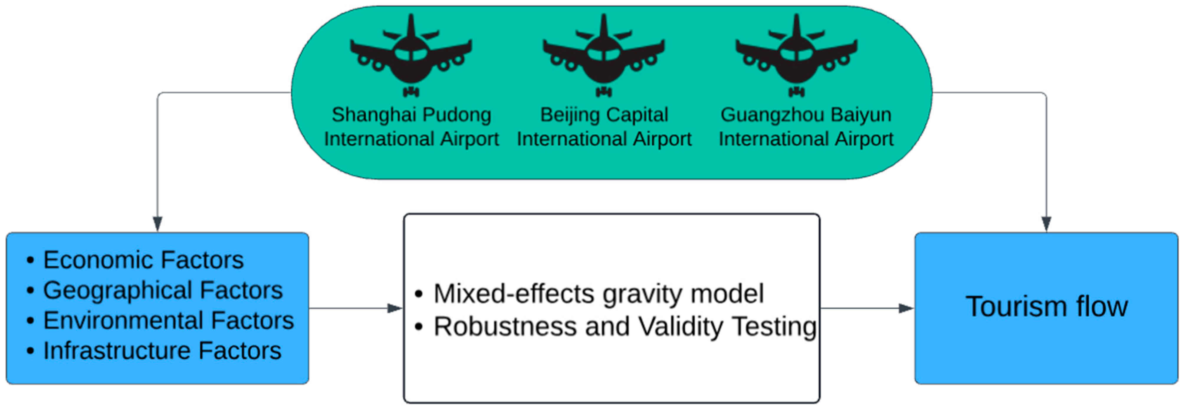
• Geographical Location: Proximity to major entry points is crucial. The study quantifies geographical advantage by the distance from provincial capitals to Beijing, Shanghai, or Guangzhou, denoted by D.
• Tourism Resources: The quality and density of tourism attractions are operationalized through the prevalence of scenic spots rated 4A-grade and above, which signify competitive tourism assets, denoted by AA.
• Traffic Conditions: This study assesses the transportation network using road density, an essential component of the tourism value chain, denoted by TRA, reflecting the region’s accessibility.
• Tourism Services: Service capacity is gauged by the number of star-rated hotels, denoted by S, a surrogate for service quality and availability.
• Traffic Safety: Traffic safety, a significant factor for destination image, is measured by traffic accident mortality density, denoted by SS.
• Environmental Protection: The ecological variables include wastewater and solid waste discharge densities alongside urban green space, capturing the role of ecological stewardship in tourism, denoted by IW, IS, and GR, respectively.

This approach delineates the economic levers of inbound tourism, spotlighting areas for policy intervention to enhance the sector’s performance. By focusing on actionable economic variables, the study provides a robust framework for policymakers to direct investments and regulatory efforts to foster a resilient and attractive tourism market.

Taking logarithms on both sides of the model, we obtain the panel data model for tourism attraction through the formula

$$\begin{array}{rr}& \log \left(T_{ij}\right)={\alpha }_{it}+{\alpha }_1\log \left(Y_{it}\right)+{\alpha }_2\log \left(D_i\right)+{\alpha }_3\log \left(A{A}_i\right)+{\alpha }_4\log \left(TR{A}_{it}\right)+\\ & {\alpha }_5\log \left(S_{it}\right)+{\alpha }_6\log \left(S{S}_{it}\right)+{\alpha }_7\log \left(I{W}_{it}\right)+{\alpha }_8\log \left(I{S}_{it}\right)+{\alpha }_9\log \left(G{R}_{it}\right)+{\mu }_{it}\end{array}$$

(4)

where ${\alpha }_{it}$ reflects the differences among the regions at different times. To calculate each ${\alpha }_{it}$ we use the least squares method, which minimizes the sum of the squares of the residuals, making it possible to obtain the best unbiased estimates under Gauss–Markov assumptions. Adopting such an econometric model has numerous benefits, including effectively increasing the sample size, reducing multicollinearity, and estimating the impact of difficult-to-measure factors on the dependent variable. As a result, the tourism attraction panel data model developed in this study is more effective at measuring the impact of various factors on the development of China’s inter-provincial inbound tourism industry.

This study expects the signs of ${\alpha }_1,{\alpha }_3,{\alpha }_4,{\alpha }_5$ and ${\alpha }_9$ to be positive and the signs of ${\alpha }_2,{\alpha }_6,{\alpha }_7$ and ${\alpha }_8$ to be negative for the parameters in the model. Economic development, the availability of tourism resources, transportation infrastructure, tourism service facilities, and environmental greening all contribute to the growth of regional inbound tourism, while challenges such as regional remoteness, poor security, and environmental pollution need to be addressed to improve the development of regional inbound tourism.

3.2. Econometric Analysis

To analyze inter-provincial tourism flows within China, we utilize a sophisticated econometric framework that applies a time-fixed effect regression model to robustly investigate the impacts of socio-economic, infrastructural, and environmental factors. This model is chosen for its ability to control for unobserved heterogeneity across time, ensuring that the variations due to the independent variables are accurately isolated. The Heckman two-step correction method is implemented to correct for potential sample selection biases, which could arise from the non-random selection of provinces included in the study. This method adjusts for biases by initially modeling the probability of each province’s inclusion in the sample and correcting the main regression analysis accordingly.

The validity of our model is rigorously tested through several methods. Cross-validation is conducted by comparing the model’s predictions against actual tourism data, which helps verify the model’s predictive accuracy and the reliability of its estimates. Sensitivity analysis is also performed to assess the stability of the regression coefficients when varying key parameters, ensuring that the findings are not overly sensitive to specific assumptions. Hypothesis testing is an integral part of our analysis. The Hausman test is utilized to determine the appropriateness of fixed versus random effects based on whether the unique errors in the model are correlated with the regressors. Additionally, F-statistics are calculated to confirm the overall significance of the regression model, ensuring that all explanatory variables collectively influence the dependent variable.

To further substantiate the reliability of our findings, robustness checks are carried out, including stationarity tests to ensure that the data do not suffer from unit root problems, which could lead to spurious regression results. Multicollinearity tests are also conducted to ensure no excessive correlation among the independent variables, which could undermine the statistical validity of the model. These methodological steps not only bolster the credibility of the analytical results but also enhance the practical utility of the model for informing targeted policy interventions aimed at optimizing tourism development across China’s provinces.

4. Analysis Results and Discussion

4.1. Data and Statistical Testing

4.1.1. Data Variables and Description

This study selects 31 provinces and municipalities in China (excluding Taiwan, Hong Kong, and Macau) as research subjects, with sample data spanning from 1997 to 2019. The descriptions of the main variables are as follows:

• Per capita real GDP (year): prices were adjusted from 1990 to reflect per capita GDP and the GDP deflator index, which is calculated using the per capita and capita GDP indexes from the ‘China Statistical Yearbook’.
• Geographical location variable (D): The shortest distance between each province’s capital and Beijing, Shanghai, and Guangzhou, respectively, is calculated, with Beijing’s, Shanghai’s, and Guangzhou’s D values set to zero. Distance information is obtained from the mileage query tool on the train ticket website (http://search.huochepiao.com).
• Tourism resources: this includes the number of 5A and 4A scenic spots in each province, as reported by the National Ministry of Culture and Tourism (https://www.mct.gov.cn/) and on provincial culture and tourism departments’ official websites.
• Transportation and environmental factors: These include highway mileage, the number of traffic fatalities, total wastewater discharge, total industrial solid waste discharge, and green coverage area. For the years of the study, these figures have been obtained from the ‘China Statistical Yearbook’.
• Tourism facilities: the number of star-rated hotels is based on the ‘China Statistical Yearbook’ and ‘China Tourism Statistics Yearbook’.

Table 2. Descriptive statistics for 2019 data by region.

Variables	Unit	Mean	Maximum (Region)	Minimum (Region)	Standard Deviation
Inbound Tourist Numbers	Ten Thousand Person-Times	392.9	3731.39 (Guangdong)	7.31 (Qinghai)	645.86
2. Per Capita GDP	Yuan	36,023.4	324,633.79 (Inner Mongolia)	12,015.91 (Guizhou)	54,317.64
3. Regional Area	Ten Thousand Square Kilometers	31.0	166.00 (Xinjiang)	0.63 (Shanghai)	38.70
4. Distance	Kilometers	1026.4	3753 (Tibet)	0 (Beijing, etc.)	868.13
5. Highway Mileage	Kilometers	161,693.4	337,095 (Sichuan)	13,045 (Shanghai)	83,846.86
6. Total Number of Star-rated Hotels	Units	286	586 (Guangdong)	71 (Tianjin)	129.12
7. Number of 4A-Level and Above Attractions	Units	149.1	341 (Sichuan)	27 (Tibet)	79.56
8. Total Industrial Solid Waste Emissions	Ten Thousand Tons	11,441.6	38,574.74 (Shanxi)	473.99 (Beijing)	10,015.19
9. Wastewater Discharge	Ten Thousand Tons	37,672.4	149,661 (Fujian)	253 (Tibet)	41,946.13
10. Traffic Accident Fatalities	Persons	2024.6	4932 (Guangdong)	137 (Tibet)	1313.28
11. Green Coverage Area	Hectares	117,862.9	584,449 (Guangdong)	6415 (Tibet)	111,740.90

presents the results of descriptive statistics. Guangdong had the highest number of inbound tourists at 37.3139 million, while Qinghai had the lowest at 0.0731 million. Inner Mongolia had the highest per capita GDP of CNY 324,633, while Guizhou had the lowest at CNY 12,015. Sichuan had the longest highway mileage at 337,095 km, while Shanghai had the shortest at 13,045 km. Guangdong had the most star-rated hotels, with 586, whereas Tianjin had the least at 71. Shanxi had the highest total industrial solid waste discharge of 38,574.74 thousand tons, whereas Beijing had the lowest at 473.99 thousand tons. The region with the highest number of traffic accident deaths in China was Guangdong, with 4932 fatalities, while Tibet had the lowest with 137. Regarding green coverage area, Guangdong was also the highest, with 584,449 hectares, while Tibet had the smallest, with 6415 hectares.

4.1.2. Stationarity Test

The purpose of this study is to ensure the reliability of the panel data model and to avoid spurious regression by performing unit root tests on the variables. To improve the credibility of the results, four different testing methods are used: the Levin, Lin, and Chu test, the Im, Pesaran, and Shin W-stat test, the augmented Dickey-Fuller–Fisher Chi-square test, and the Phillips–Perron–Fisher Chi-square test. It is worth noting that because the geographical location variable (D) and the tourism resource variable (AA) are both constant across regions, they are not subject to stationarity tests [22]. The unit root test results are summarized in

Table 3. Root test results for each variable unit.

Sequence Testing Statistics	Levin, Lin & Chut *	Im, Pesaran and Shin W-Stat	ADF-Fisher Chi-Square	PP-Fisher Chi-Square	Result
log(T)	−1.6480 **	−4.4338 ***	−0.5362	3.0107 ***	Non-stationary
D(log (T))	−6.1905 ***	−14.1404 ***	16.4889 ***	50.2929 ***	stationary
log (Y)	−2.8277 ***	−0.3048	−1.7325	−2.3106	Non-stationary
D(log (Y))	−5.2523 ***	−9.1162 ***	4.0465 ***	13.1991 ***	stationary
log (TRA)	−4.2495 ***	−3.5572 ***	2.1402 **	0.1201	Non-stationary
D(log (TRA))	−10.299 ***	−13.1237 ***	17.9040 ***	35.4777 ***	stationary
log (S)	−5.4847 ***	−7.3499 ***	5.1900 ***	8.8451 ***	stationary
D(log (S))	−12.1940 ***	−15.5096 ***	30.6397 ***	69.1505 ***	stationary
log (IS)	−3.7170 ***	−6.8985 ***	1.8741 **	7.1360 ***	stationary
D(log (IS))	−10.1280 ***	−14.4749 ***	26.7941 ***	56.6750 ***	stationary
log (IW)	−1.0934	−2.7487 ***	−0.4335	0.0509	Non-stationary
D(log (IW))	−6.2272 ***	−13.4863 ***	13.5708 ***	41.2912 ***	stationary
log (SS)	−2.9336 ***	−2.9626 ***	2.3891 ***	0.6059	Non-stationary
D(log (SS))	−9.2792 ***	−13.4447 ***	23.6228 ***	43.8997 ***	stationary
log (GR)	−4.4323 ***	−3.5962 ***	0.1039	2.8353 ***	Non-stationary
D(log (GR))	−12.2317 ***	−11.1152 ***	18.7469 ***	36.8361 ***	stationary

Note: D() indicates the differenced series; * signifies significance at the 10% level; ** indicates significance at the 5% level; *** denotes significance at the 1% level.

.

Our analysis reveals that several key variables in their original forms exhibit non-stationarity, suggesting the presence of trends or seasonal effects that could distort regression outcomes. For instance, variables such as Log(T) (tourism numbers), Log(Y) (economic output), Log(TRA) (transportation infrastructure), Log(IW) (industrial waste), Log(SS) (safety and security), and Log(GR) (green coverage) initially failed to reject the unit root null hypothesis, indicating non-stationarity. However, all these variables attain stationarity once differenced, as evidenced by significant test statistics across all respective tests for the differenced series. This transformation underscores the necessity of differencing to stabilize the mean and variance of the series, thereby making them suitable for inclusion in regression analysis.

Conversely, variables like Log(S) (service quality) and Log(IS) (solid waste management) display stationarity in their original forms, suggesting that they do not contain trends or seasonal effects that would necessitate differencing. This characteristic makes them directly applicable to the regression models, simplifying the modeling process and ensuring the integrity of the econometric analysis.

The incorporation of these stationarity tests and the subsequent transformations of the data provide a robust foundation for the empirical analysis. By ensuring that all variables used in the regression models are stationary, the study effectively mitigates the risk of spurious relationships, enhancing the validity and reliability of the findings. This methodological rigor not only strengthens the study’s conclusions but also aligns with best practices in econometric analysis, ensuring that the insights derived from the study are well-founded and scientifically robust.

4.1.3. Correlation Analysis

This study examines the relationships between different variables using the correlation matrix before validating the model (see

Table 4. The results of the correlation analysis.

	T	Y	D	AA	TRA	S	SS	IW	IS	GR
T	1
Y	0.601 ***	1
D	−0.528 ***	−0.429 ***	1
AA	0.507 ***	0.293 ***	−0.616 ***	1
TRA	0.651 ***	0.565 ***	−0.450 ***	0.817 ***	1
S	0.752 ***	0.355 ***	−0.360 ***	0.405 ***	0.554 ***	1
SS	0.485 ***	0.252 ***	−0.646 ***	0.948 ***	0.751 ***	0.427 ***	1
IW	0.490 ***	0.250 ***	−0.552 ***	0.931 ***	0.765 ***	0.448 ***	0.927 ***	1
IS	0.479 ***	0.465 ***	−0.409 ***	0.779 ***	0.823 ***	0.445 ***	0.721 ***	0.785 ***	1
GR	0.774 ***	0.530 ***	−0.395 ***	0.534 ***	0.678 ***	0.728 ***	0.522 ***	0.583 ***	0.633 ***	1

*** denotes significance at the 1% level.

). According to the results shown in Table 4, the dependent variable ‘inbound tourist numbers’ has a significant positive correlation at the 1% level with the following variables: level of economic development, the density of 4A-level and above tourist attractions, road network density, number of star-rated hotels, traffic accident death density, wastewater discharge density, industrial solid waste discharge density, and green coverage area. These results suggest that the number of tourists in each province and the explanatory variables are positively correlated.

However, a statistically significant negative correlation exists between tourist numbers and the shortest straight-line distance to the capital cities from Beijing, Shanghai, and Guangzhou, respectively, at the 1% level. This indicates a negative relationship between tourist numbers and geographic distance. The positive correlations between tourist numbers and traffic accident death density, wastewater discharge density, and industrial solid waste discharge density contradict theoretical expectations. This could be because the correlation analysis did not account for the effects of other variables and only examined the relationships between two variables. Therefore, a third variable may influence these positive correlations, and the results do not always reflect the true relationship between the two variables.

4.2. Model Selection and Estimation

The panel data models used in this study are predominantly mixed and fixed-effect models. Because policy implementation and tourism resources vary significantly across regions, cross-sectional units are not considered samples from the same population. Instead, mixed and fixed-effect models are employed, typically including individual-fixed, time-fixed, and individual-time-fixed effect models. Individual effects are ignored in model (4) because the distance variable (D) and the tourism resource variable (AA) are fixed for each region.

Statistical measures like cap R squared and t-values cannot be used to compare the estimation results of the time-fixed effects and mixed-effects regression models. As a result, an F-statistic must be calculated using the ratio between the sums of squared residuals from the unconstrained and constrained models. The null hypothesis H_O is that the intercepts in the model are the same at different time points (the actual model is the mixed regression model), and the alternative hypothesis H₁ is that the intercept terms differ at different time points (the actual model is the time-fixed effects regression model). Under the null hypothesis (H₀), the F-statistic is constructed as

$$F={\displaystyle \frac{\left(SS{R}_r-SS{R}_u\right)/(T-1)}{SS{R}_u/(NT-T-k)}}\sim F(T-1,NT-T-k)$$

(5)

where $SS{R}_r$ represents the sum of the squared residuals of the mixed regression model, $SS{R}_u$ represents the sum of the squared residuals of the time-fixed effects regression model, $T$ is the length of the periods, and k is the number of explanatory variables. The mixed- and time-fixed effect regression models for model (4) are estimated, and the results are presented in

Table 5. Estimation results of panel data model (4).

Explanatory Variable	Mixed-Effects Regression Model	Time-Fixed Effects Regression Model
Constant	−8.7534 *** (0.6314)	−13.6011 *** (0.9954)
LOG(Y)	0.4653 *** (0.0595)	0.8792 *** (0.0871)
LOG(D)	−0.0950 *** (0.0230)	−0.0556 ** (0.0229)
LOG(AA)	0.4105 *** (0.1019)	0.3641 *** (0.1004)
LOG(TRA)	0.2489 *** (0.0810)	0.6303 *** (0.1009)
LOG(S)	0.7447 *** (0.0639)	0.8157 *** (0.0681)
LOG(SS)	−0.2002 ** (0.0815)	−0.3173 *** (0.0896)
LOG(IW)	−0.0241 (0.0520)	−0.1609 *** (0.0614)
LOG(IS)	−0.2680 *** (0.0357)	−0.2162 *** (0.0356)
LOG(GR)	0.4735 *** (0.0527)	0.4706 *** (0.0557)
N	589	589
R2	0.77	0.79
residual sum of squares	311.25	273.22
F Statistics	216.99 ***	82.73 ***

Note: Values in brackets are standard errors. ** indicates significance at the 5% level; *** denotes significance at the 1% level.

.

Table 5 shows that the calculated F-value is 4.34, significantly higher than the 5% level critical value of $F_{0.05}\left(\mathrm{18,561}\right)=1.62.$ Therefore, establishing a time-fixed effects model makes more sense. Columns (1) and (2) of Table 5 show the estimated results of the panel mixed regression model and the time-fixed effects model with year dummy variables, respectively. When the two columns are compared, the negative impact of wastewater discharge density on tourism is found to be statistically significant in column (2) but not in column (1). In contrast, the significance and direction of the impact of other variables are nearly identical in both columns.

According to the primary model’s estimated results in column (2), increasing per capita GDP, the density of 4A-level and above tourist attractions, road network density, the number of star-rated hotels, and green coverage areas can all significantly increase the number of inbound tourists in a province. In contrast, geographic distance, traffic accident death density, wastewater discharge density, and industrial solid waste discharge density can significantly reduce the number of inbound tourists in each province. The constructed inbound tourism attraction model explains 79% of the total variation in inbound tourist numbers. The t-statistic shows that all explanatory variables significantly impact the dependent variable at the 5% significance level. The F-statistic shows that the combined effect of the model’s explanatory variables on the dependent variable is also significant at the 1% level.

4.3. Establishing the Cluster-Based Portfolios

To ensure the reliability of the above-mentioned conclusions, this section of the study uses truncation methods to exclude outliers during model-robustness testing. Compared to previous estimates, truncation occurs at the 1% and 99% levels, rather than tail-trimming. Although this method reduces the sample size, it effectively eliminates extreme values.

The robustness test results in

Table 6. Robustness test results.

Explanatory Variable	Robustness Test
Constant	−11.4732 *** (0.9125)
LOG(Y)	0.6510 *** (0.0708)
LOG(D)	−0.0814 *** (0.0229)
LOG(AA)	0.2949 *** (0.1025)
LOG(TRA)	0.6167 *** (0.1031)
LOG(S)	0.8544 *** (0.0686)
LOG(SS)	−0.2311 *** (0.0896)
LOG(IW)	−0.1013 *** (0.0611)
LOG(IS)	−0.2675 *** (0.0362)
LOG(GR)	0.4015 *** (0.0533)
N	521
R2	0.78
residual sum of squares	291.01
F Statistics	78.20 ***

Note: Values in brackets are standard errors. *** denotes significance at the 1% level.

are consistent with earlier model outcomes, confirming the reliability of the initial conclusions. The constant term (C) shows a significant negative value, suggesting that tourism growth might naturally decline without proactive measures. The positive coefficient for LOG(Y), which represents economic development, indicates a strong link between increased per capita GDP and tourism inflow, highlighting economic prosperity as a crucial driver of tourism.

Furthermore, the negative coefficient for LOG(D) underscores the importance of geographical proximity to urban centers in attracting tourists, emphasizing the need for accessible tourism planning. The positive values for LOG(AA) and LOG(TRA), representing tourism resources and transportation infrastructure, respectively, confirm that these factors significantly enhance tourist numbers, suggesting that investments in quality attractions and accessibility improvements are beneficial. LOG(S), which indicates service quality, also shows a positive and significant impact on tourism, reinforcing the idea that high-quality services are vital for attracting tourists. Conversely, negative coefficients for LOG(SS), LOG(IW), and LOG(IS), which denote safety and security, industrial waste, and solid waste, respectively, indicate that higher rates of traffic fatalities and greater waste production negatively affect tourism numbers. These findings highlight the need to improve safety standards and environmental management practices.

Lastly, the positive impact of LOG(GR), representing green coverage, demonstrates that increasing green spaces enhances the aesthetic appeal of a destination and its overall attractiveness to tourists. This supports integrating environmental sustainability into tourism development strategies.

Environmental protection measures are crucial for sustainable tourism development, yet they present a complex dual impact on the tourism industry. On the positive side, environmental protection efforts, such as enhancing green coverage and reducing pollution, can significantly boost a destination’s attractiveness. For example, increasing urban green spaces not only improves the aesthetic appeal but also enhances the overall visitor experience by providing cleaner and healthier environments. Regions with higher green coverage have been shown to attract more tourists due to their perceived commitment to sustainability and natural beauty. For example, in Zhangjiajie National Forest Park, initiatives to increase forest coverage and reduce air pollution have made the park more attractive, leading to a significant increase in visitor numbers.

Conversely, certain environmental protection measures can have negative implications for tourism. Stricter regulations and conservation efforts might lead to increased operational costs for tourism businesses. For example, limitations on tourist activities in protected areas to prevent ecological damage can reduce the availability of popular attractions. The implementation of pollution control measures may require significant investments from local businesses, potentially increasing costs for tourists. An example of this negative impact is seen in certain coastal areas where stringent fishing regulations to protect marine life have restricted traditional fishing tours, thereby decreasing tourist activities and affecting local tourism revenue.

In summary, while environmental protection measures are essential for the long-term sustainability of tourism, they must be carefully balanced with the economic needs of the tourism industry. Policymakers should aim to implement strategies that mitigate negative impacts while enhancing the positive effects of environmental conservation.

Overall, the robustness checks validate that the model’s findings are reliable and applicable across typical scenarios in provincial China. The key drivers identified—economic factors, infrastructure quality, service excellence, and environmental management—should be integral to regional planning and national tourism strategies to foster sustainable tourism growth.

4.4. Heterogeneity Test

This study explores the heterogeneous impact of various economic, geographical, and environmental factors on tourism across Chinese provinces, categorized by their levels of economic development. Utilizing median annual per capita GDP, regions were divided into developed and less developed areas to ascertain the differential effects of these factors on tourism.

Our analysis, summarized in

Table 7. Heterogeneity test results.

Explanatory Variable	Developed Areas	Less Developed Areas
Constant	−9.3849 *** (1.2106)	−15.0937 *** (2.8415)
LOG(Y)	0.7664 *** (0.0992)	1.5105 *** (0.2820)
LOG(D)	−0.1685 *** (0.0159)	−0.1222 (0.1372)
LOG(AA)	−0.4427 *** (0.0956)	1.1658 *** (0.1866)
LOG(TRA)	0.3271 *** (0.0978)	0.4972 *** (0.1588)
LOG(S)	0.5438 *** (0.0640)	1.4402 *** (0.1144)
LOG(SS)	−0.1117 (0.0840)	−0.4219 ** (0.1638)
LOG(IW)	0.3953 *** (0.0633)	−0.4709 *** (0.0927)
LOG(IS)	−0.3158 *** (0.0375)	−0.2333 *** (0.0674)
LOG(GR)	0.2267 *** (0.0569)	0.1515 (0.1083)
N	285	285
R2	0.87	0.77
F Statistics	69.39 ***	37.01 ***

Note: Values in brackets are standard errors. ** indicates significance at the 5% level; *** denotes sig-nificance at the 1% level.

, reveals insightful disparities between developed and less developed regions. In less developed areas, the constant term is more negative (−15.0937 compared to −9.3849 in developed areas), indicating a lower baseline for tourism attractiveness. This suggests substantial inherent challenges that may hinder tourism growth in these regions. The effect of economic development (LOG(Y)) on tourism is notably stronger in less developed areas (1.5105) than in developed ones (0.7664), demonstrating that economic growth could significantly boost tourism in economically lagging regions.

Geographical distance (LOG(D)) adversely affects tourism in all regions. Still, it is less impactful in less developed areas, implying that distance is a less critical factor due to lower baseline expectations or different competitive dynamics in these regions. Tourism resources (LOG(AA)) present an intriguing contrast; they negatively impact developed areas but have a significant positive effect in less developed areas. This indicates potential for growth from new attractions in less developed regions, where the tourism market is not yet saturated.

Transportation infrastructure (LOG(TRA)) also positively impacts both groups, though the effect is more pronounced in less developed areas. This underscores the importance of improving accessibility to enhance tourism, particularly in areas with underdeveloped infrastructure. Service quality (LOG(S)) significantly boosts tourism more in less developed areas, suggesting that enhancing service quality there can yield disproportionately high benefits, likely due to current lower levels of service provision.

This analysis also highlights universal concerns such as safety and security (LOG(SS)), which negatively impact tourism across all regions, with a stronger deterrent effect in less developed areas. Environmental factors exhibit contrasting impacts; industrial waste (LOG(IW)) has a positive effect in developed areas but a negative one in less developed regions, reflecting differing levels of industrial activity and its acceptance by tourists. Solid waste management (LOG(IS)) poses a more significant issue in less developed areas, underscoring the need for improved waste management practices to enhance tourism appeal.

In conclusion, the heterogeneity analysis provided by this study offers vital insights into the varying impacts of developmental, infrastructural, and environmental factors on tourism across regions with different economic statuses. These findings can inform targeted policy interventions, ensuring that strategies are tailored to meet the specific needs and conditions of each region, thereby promoting balanced regional tourism development and sustainable economic growth.

4.5. Empirical Results

This study’s empirical analysis, utilizing a time-fixed effect regression model, provides new quantitative insights that distinguish and extend the understanding of factors shaping inbound tourism across China’s diverse regions. Our findings demonstrate a significant relationship between economic prosperity and tourism growth, revealing a more nuanced interaction than previously reported. For instance, while the general correlation aligns with findings by Cortes-Jimenez and Pulina [1], our study refines this by quantifying the impact: a 1-percentage-point increase in per capita GDP leads to a 0.88 percentage point rise in inbound tourist numbers, showcasing a direct linkage between economic vitality and tourism that builds on the foundational work of Zhou [2].

Moreover, geographic proximity to major urban centers such as Beijing, Shanghai, and Guangzhou are critical in attracting tourists. This research quantifies the decremental impact of increased distance, where every additional 100 km reduces tourist numbers by 5.56 percentage points, a finding that further develops the concepts introduced by Hanafiah et al. [23] and Guo [14]. Unlike prior studies that broadly highlighted proximity’s importance, our model provides specific, actionable data that can inform regional planning and marketing strategies.

This study also highlights the significance of infrastructure, particularly the density of 4A-level attractions, as a major driver of tourism. This extends the observations of Zhang et al. [15] and Li et al. [16] by showing that infrastructure improvements in underdeveloped areas correlate strongly with substantial increases in tourism. This suggests that targeted infrastructure investments could be a potent mechanism for regional development.

Our analysis further emphasizes the critical role of public safety and environmental sustainability in supporting tourism growth. This priority has become increasingly important, as noted by Rossello Nadal et al. [11]. Negative externalities such as traffic fatalities and environmental pollution significantly deter tourism, underscoring the need for integrated policy approaches that encompass environmental management and public safety. A novel aspect of this study is the identification of regional disparities in how attractions and infrastructure impact tourism numbers. Developed and developing areas exhibit markedly different dynamics, which challenges the one-size-fits-all approach often assumed in tourism development. This supports the call by Wang [17] and Liu et al. [18] for differentiated strategies that consider the economic and geographic diversity of regions.

By integrating these findings, this research contributes distinctively to the field of tourism economics by reinforcing established theories and offering new empirical evidence that facilitates more informed decision-making for sustainable tourism development. The insights here emphasize the need for regionally tailored strategies that ensure sustainable growth while addressing development-level disparities.

5. Discussion

The findings of this study provide significant insights into the dynamics of inbound tourism in China, highlighting the critical interplay between economic factors, geographic proximity, and environmental conditions. Using a mixed-effects gravity model, we found that a 10% increase in per capita GDP results in a 0.88% rise in inbound tourist numbers, reinforcing the role of economic development in driving tourism growth. This result is consistent with previous studies, such as Cortes-Jimenez and Pulina, who found that economic growth positively impacts tourism demand [1]. Similarly, Zhou highlighted the importance of economic development in boosting tourism activities [2].

Our study also quantifies the impact of geographic distance on tourism, showing that every 100 km increase in distance from major urban centers like Beijing, Shanghai, and Guangzhou leads to a 5.56% decrease in tourist arrivals. This underscores the importance of accessibility and transportation infrastructure, corroborating the findings of Hanafiah et al. [23] and Guo [14], who emphasized the role of geographic proximity and transportation networks in facilitating tourism flows.

Hypothesis testing is an integral part of our analysis. The hypotheses were tested using the gravity-based regression model. The results provide robust evidence for the proposed hypotheses:

• H1: Economic development, as indicated by the positive coefficient for LOG(Y), confirms that higher per capita GDP significantly increases inbound tourist numbers. This supports the hypothesis that economic factors positively impact tourism, aligning with findings from studies by Cortes-Jimenez and Pulina [1] and Zhou [2].
• H2: The negative coefficient for LOG(D) confirms that greater geographical distance from major urban centers significantly reduces tourist numbers, supporting the hypothesis that geographical proximity influences tourism. This is consistent with the work of Hanafiah et al. [23] and Guo [14], who also found that proximity to major cities enhances tourism activities.
• H3: Environmental factors such as green coverage (LOG(GR)) and reductions in industrial waste (LOG(IW)) positively affect inbound tourism. The positive coefficients for these variables confirm that environmental improvements enhance destination attractiveness, supporting the hypothesis that environmental factors positively influence tourism. This finding extends the work of Buckley [24] and Gössling [25], who highlighted the importance of environmental sustainability in tourism development.
• H4: The dual impact of environmental protection measures is observed. While improvements in environmental quality (e.g., increased green coverage) positively attract tourists, stricter regulations and conservation efforts can lead to increased operational costs and reduced availability of popular attractions. For instance, stringent fishing regulations in certain coastal areas have restricted traditional fishing tours, thereby decreased tourist activities and affected local tourism revenue. This confirms the hypothesis that environmental protection measures can have both positive and negative impacts on tourism. These findings are in line with the work of Buckley [24], who noted the potential trade-offs between environmental conservation and tourism development.

The dual impact of environmental factors is another key finding. Improvements in green coverage and reductions in industrial waste and traffic fatalities positively influence tourist arrivals. However, stringent environmental protection measures may sometimes deter tourism activities or increase operational costs. This complexity suggests that policymakers need to carefully balance environmental sustainability with tourism development. Despite the robustness of our model, which explains 79% of the variability in inbound tourism flows, several limitations exist. The reliance on available statistical data may not capture all nuances of tourism dynamics, such as cultural factors or tourist preferences. Future research should incorporate more qualitative data and explore tourism dynamics in a broader range of locations.

In conclusion, this research offers valuable strategic insights for policymakers and stakeholders in the tourism sector. Integrating economic and environmental strategies can enhance a region’s attractiveness and sustainability, fostering a more resilient tourism industry. Future studies should continue to explore the complex interactions among the various factors influencing tourism to develop more comprehensive and adaptive models for sustainable tourism development.

6. Conclusions

The research presented in this study offers substantial theoretical and practical advancements in the field of tourism economics by refining the gravity model through the inclusion of multi-dimensional factors. These advancements are classified into theoretical and practical implications to facilitate clear understanding and straightforward application.

6.1. Theoretical Implications

This study’s theoretical contribution lies in its enhancement of the gravity model, incorporating economic, geographical, and environmental factors. This advancement extends the scholarly discussion and opens new research avenues in tourism economics. The enhanced model facilitates a comprehensive analysis of the interplay between these variables and their influence on tourism patterns.

Specifically, the study emphasizes the significant impact of economic development, social security, environmental protection, and robust infrastructure on driving tourism growth. These findings align with contemporary regional development economic theories, illustrating how economic growth significantly boosts tourism activities. Additionally, the research highlights the critical role of social security measures in creating a favorable environment for tourism.

Environmental protection emerges as another vital factor, particularly the expansion of green spaces, which significantly enhances regional tourism attractiveness. The study also underscores the importance of robust infrastructure, such as transportation and accommodation facilities, in facilitating tourism flows. By integrating these diverse elements, the theoretical framework provided by this study offers a more comprehensive understanding of tourism dynamics.

6.2. Practical Implications

In addition to its theoretical contributions, the study provides substantial empirical evidence to support tourism management and policy development. These findings are crucial for policymakers and industry stakeholders aiming to promote regional economic development and sustainable tourism practices.

Firstly, the research underscores the significance of environmental quality in tourism development. Enhancements in green spaces and traffic safety can significantly boost tourist numbers, particularly in regions distant from major urban centers. These insights are valuable for policymakers integrating environmental considerations into tourism planning.

Secondly, the study advocates for strategic investments in infrastructure and tourism services. Simplifying visa processes and upgrading the quality of accommodations and dining facilities are essential for enhancing destination security and sustainability. Improving connectivity and the overall quality of tourism services can significantly elevate the appeal of tourist destinations, potentially increasing tourist satisfaction and encouraging repeat visits.

6.3. Limitations and Future Research

Despite the robustness of the model, several limitations must be acknowledged. Firstly, the study relies on available statistical data, which may not capture all nuances of tourism dynamics, such as cultural factors and tourist preferences. Secondly, the focus on urban clusters around major international airports excludes rural and less-developed areas with different tourism dynamics. Thirdly, the data spans from 1997 to 2019, not accounting for the long-term impacts of recent events like the COVID-19 pandemic. Additionally, the aggregated environmental data may not reflect local variations, limiting the accuracy of detailed insights. Finally, the study considers star-rated hotels, excluding non-star-rated and alternative accommodations, which may also affect tourism dynamics.

Future research should address these limitations better to understand China’s dynamics of inbound tourism. Incorporating qualitative data through surveys and interviews with tourists can provide valuable insights into cultural factors and preferences. Expanding the geographical scope to include rural and less-developed regions is crucial to capturing diverse tourism experiences across China.

Conducting strategic longitudinal studies extending beyond 2019 is essential for assessing the long-term impacts of events such as COVID-19 on tourism patterns. Collecting more granular, local-level environmental data will enable a more precise analysis of its specific impacts on tourism. Moreover, including non-star-rated hotels and alternative lodging options in future studies will offer a more comprehensive view of the accommodation sector’s impact on tourism.

6.4. Summary

This research lays a robust foundation for strategically integrating economic and environmental considerations into tourism policy and development. The study enhances the gravity model by incorporating key factors driving tourism growth, offering theoretical and practical contributions. The insights gained underscore the importance of interdisciplinary approaches in addressing the complexities of tourism development, particularly in the context of contemporary China. A more comprehensive understanding of inbound tourism dynamics can be achieved by addressing the identified limitations and exploring suggested areas for future research. This will guide future research and inform effective policy formulation in the field of tourism economics.

References

1. Cortes-Jimenez, I.; Pulina, M. Inbound tourism and long-run economic growth. Curr. Issues Tour. 2010, 13, 61–74. [Google Scholar] [CrossRef]
2. Zhou, P. General introduction to industrialized development of tourism since China’s Reform and Opening-Up. In The Theory and Practice of China’s Tourism Economy (1978–2017); Springer: Berlin/Heidelberg, Germany, 2019; pp. 1–31. [Google Scholar]
3. Haibo, C.; Ayamba, E.C.; Udimal, T.B.; Agyemang, A.O.; Ruth, A. Tourism and sustainable development in China: A review. Environ. Sci. Pollut. Res. 2020, 27, 39077–39093. [Google Scholar] [CrossRef]
4. Zhao, Y.; Liu, B. The evolution and new trends of China’s tourism industry. Natl. Account. Rev. 2020, 2, 337–353. [Google Scholar] [CrossRef]
5. Wang, C.; Xu, H. The role of local government and the private sector in China’s tourism industry. Tour. Manag. 2014, 45, 95–105. [Google Scholar] [CrossRef]
6. Gössling, S.; Scott, D.; Hall, C.M. Pandemics, tourism and global change: A rapid assessment of COVID-19. J. Sustain. Tour. 2020, 29, 1–20. [Google Scholar] [CrossRef]
7. Chinazzi, M.; Davis, J.T.; Ajelli, M.; Gioannini, C.; Litvinova, M.; Merler, S.; Piontti, Y.; Pastore, A.; Mu, K.; Rossi, L.; et al. The effect of travel restrictions on the spread of the 2019 novel coronavirus (COVID-19) outbreak. Science 2020, 368, 395–400. [Google Scholar] [CrossRef]
8. Crampon, L.J. A new technique to analyze tourist markets. J. Mark. 1966, 30, 27–31. [Google Scholar] [CrossRef]
9. Wilson, A.G. A statistical theory of spatial distribution models. Transp. Res. 1967, 1, 253–269. [Google Scholar] [CrossRef]
10. Ulucak, R.; Yücel, A.G.; Çil, İ.A. Dynamics of tourism demand in Turkey: Panel data analysis using gravity model. Tour. Econ. 2020, 26, 1394–1414. [Google Scholar] [CrossRef]
11. Rossello Nadal, J.; Santana Gallego, M. Gravity models for tourism demand modeling: Empirical review and outlook. J. Econ. Surv. 2022, 36, 1358–1409. [Google Scholar] [CrossRef]
12. Prezioso, M. STeMA: A Sustainable Territorial Economic/Environmental Management Approach, Advances in Spatial Science. In Territorial Impact Assessment; Medeiros, E., Ed.; Springer: Berlin/Heidelberg, Germany, 2020; Chapter 4; pp. 55–76. [Google Scholar] [CrossRef]
13. Lu, Y.H.; Liu, P.; Zhang, X.; Zhang, J.; Shen, C. Spatial-temporal differences in the effect of epidemic risk perception on potential travel intention: A macropsychology-based risk perception perspective. Sage Open 2022, 12, 21582440221141392. [Google Scholar] [CrossRef]
14. Guo, W. Inbound Tourism: An Empirical Research Based on Gravity Model of International Trade. Tour. Trib. 2007, 3, 30–34. [Google Scholar]
15. Zhang, P.; Zheng, C.Y.; Qiu, P. Empirical Study on Domestic Tourism Based on Gravity Model. Soft Sci. 2008, 22, 27–30. [Google Scholar]
16. Li, S.; Wang, Z.; Zhong, Z.Q. Gravity Model for Tourism Spatial Interaction: Basic Form, Parameter Estimation, and Applications. Acta Geogr. Sin. 2012, 67, 526–544. [Google Scholar]
17. Wang, Y. Visa Regulations and Flows of Inbound Visitors: A Gravity-Model-Based Empirical Study. Tour. Sci. 2017, 31, 17–31. [Google Scholar]
18. Liu, X.; Yang, L.; Lyu, X. The Impact of Cultural Distance on China’s Outbound Tourism: A Dynamic Panel Data Analysis Based on the Gravity Model. Tour. Sci. 2018, 4, 60–70. [Google Scholar]
19. Hunag, R.; Xie, C.-w.; Lai, F.-f. Impact of the “Belt and Road” Initiative on the Tourism Development of Destination Countries along the Route: A Empirical Test Based on Gravity Model and Difference-in-Difference Method. Geogr. Geo-Inf. Sci. 2022, 38, 120–129. [Google Scholar]
20. Zhang, Y.; Zhang, J. Revisiting Tourism Development and Economic Growth: A Framework for Configurational Analysis in Chinese Cities. Sustainability 2023, 15, 10000. [Google Scholar] [CrossRef]
21. Novotná, M.; Kubíčková, H.; Kunc, J. Beyond the buzzwords: Rethinking sustainability in adventure tourism through real travellers practices. J. Outdoor Recreat. Tour. 2024, 46, 100744. [Google Scholar] [CrossRef]
22. Abuzaid, A.; Alshqaq, S.; Elbozom, M. Statistical Modelling of Palestinian Meteorological Data Using Panel Data Techniques. ASM Sci. J. 2023, 18, 1–11. [Google Scholar] [CrossRef]
23. Hanafiah, M.H.M.; Harun, M.F.M. Tourism demand in Malaysia: A cross-sectional pool time-series analysis. Int. J. Trade Econ. Financ. 2010, 1, 200. [Google Scholar] [CrossRef]
24. Buckley, R. Sustainable tourism: Research and reality. Ann. Tour. Res. 2012, 39, 528–546. [Google Scholar] [CrossRef]
25. Gössling, S. Global environmental consequences of tourism. Glob. Environ. Chang. 2002, 12, 283–302. [Google Scholar] [CrossRef]
Figure 1. Theoretical and methodological framework.
Sustainability 16 06671 g001