
Evaluation of Coastal Ecological Security Barrier Functions Based on Ecosystem Services: A Case Study of Fujian Province, China


Abstract
:1. Introduction
2. Study Area and Data Sources
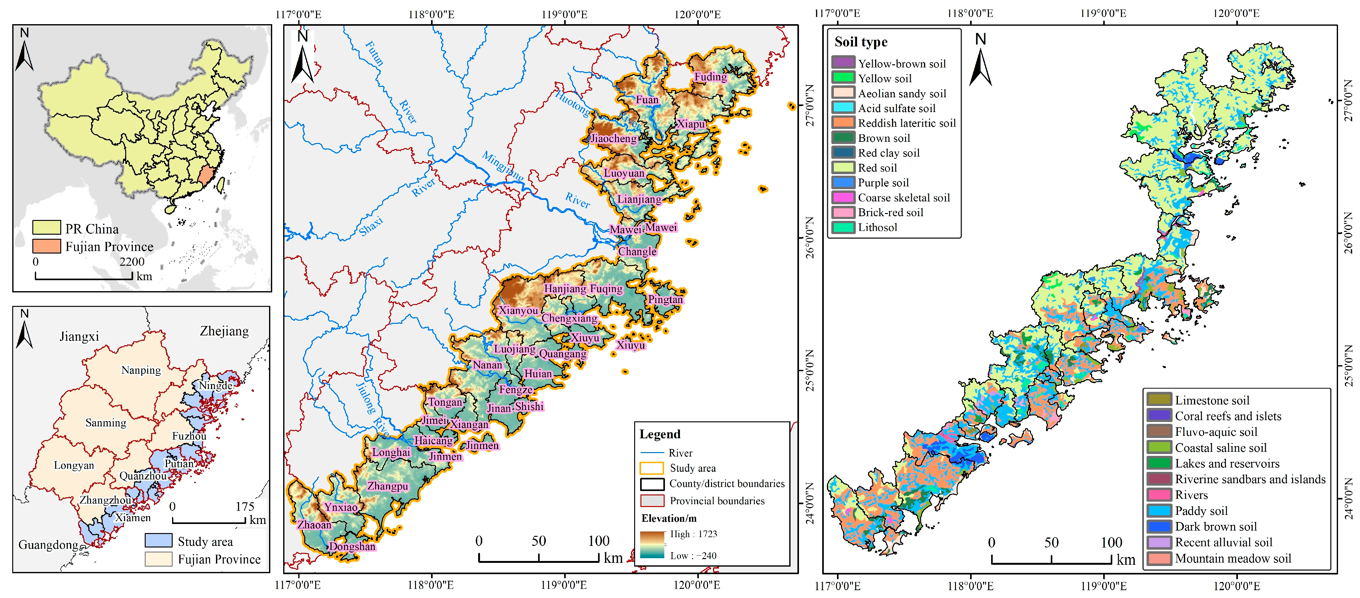
2.1. Study Area
2.2. Data Sources
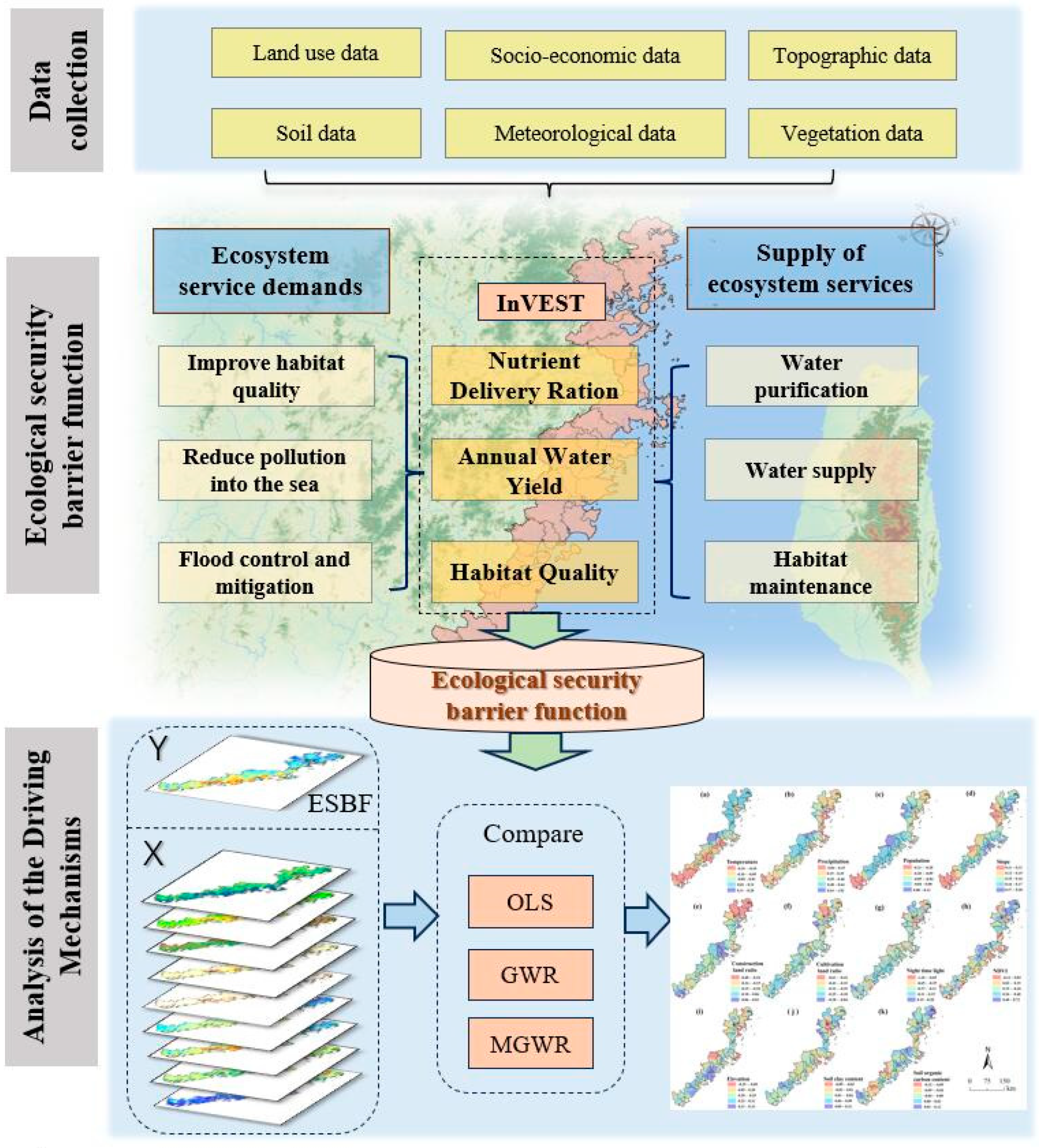
3. Methods
3.1. InVEST Modle
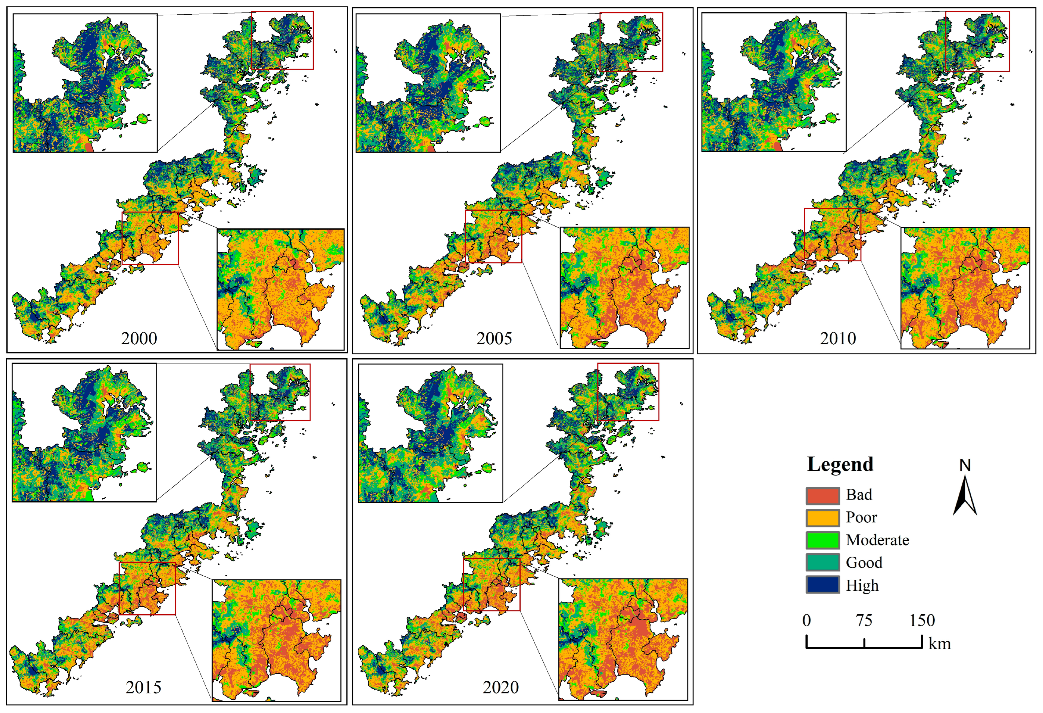
3.1.1. Habitat Quality
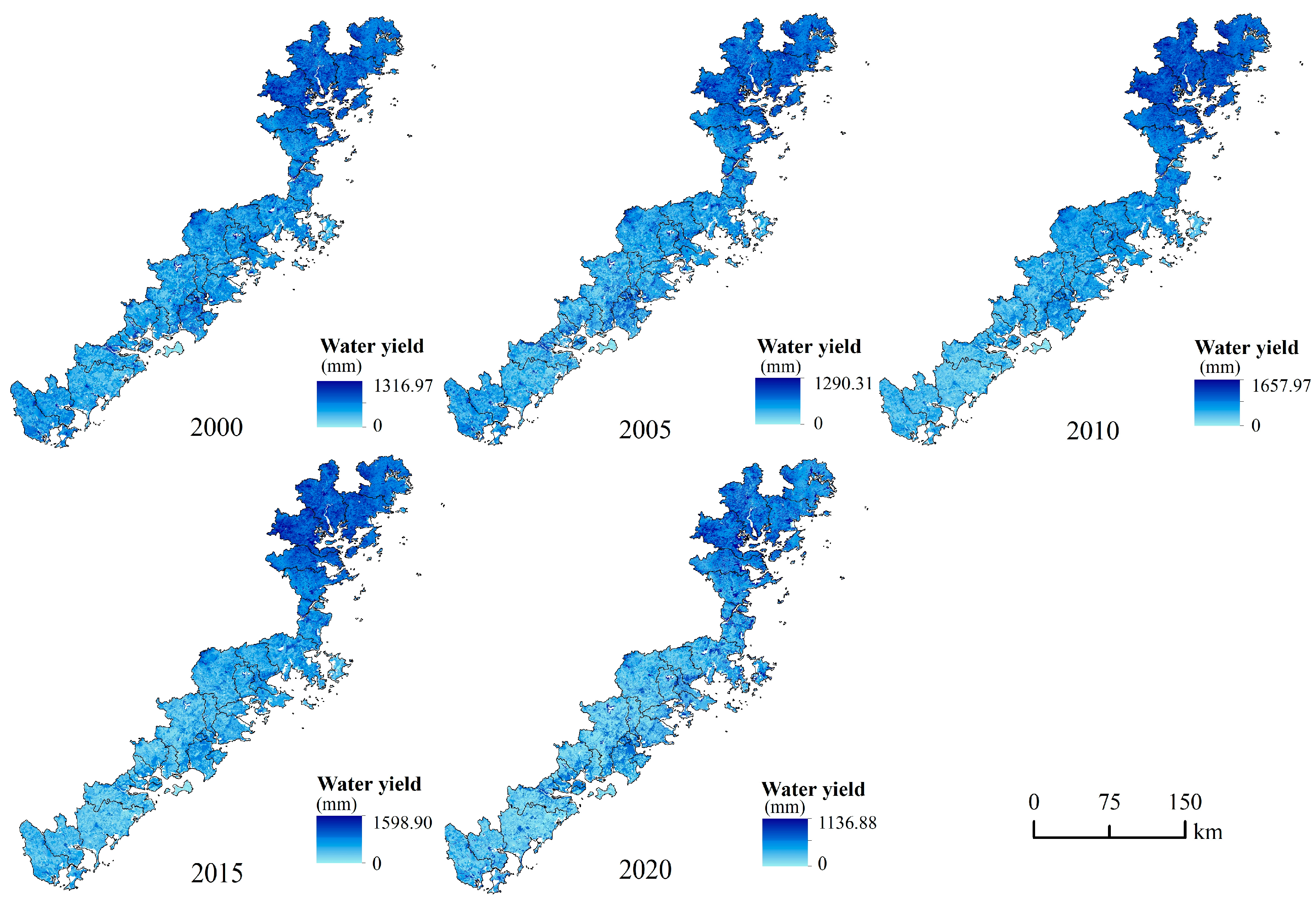
3.1.2. Annual Water Yield
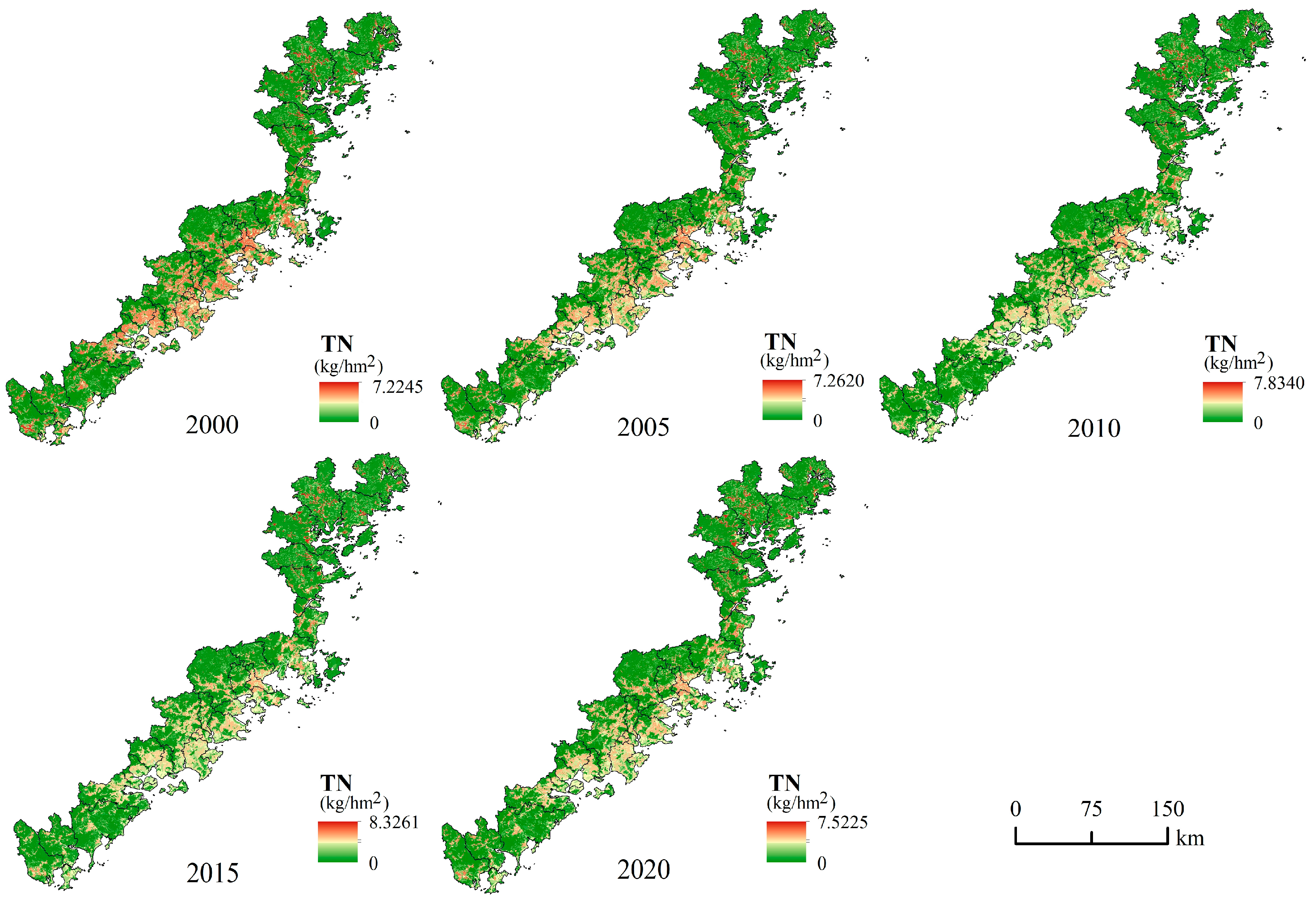
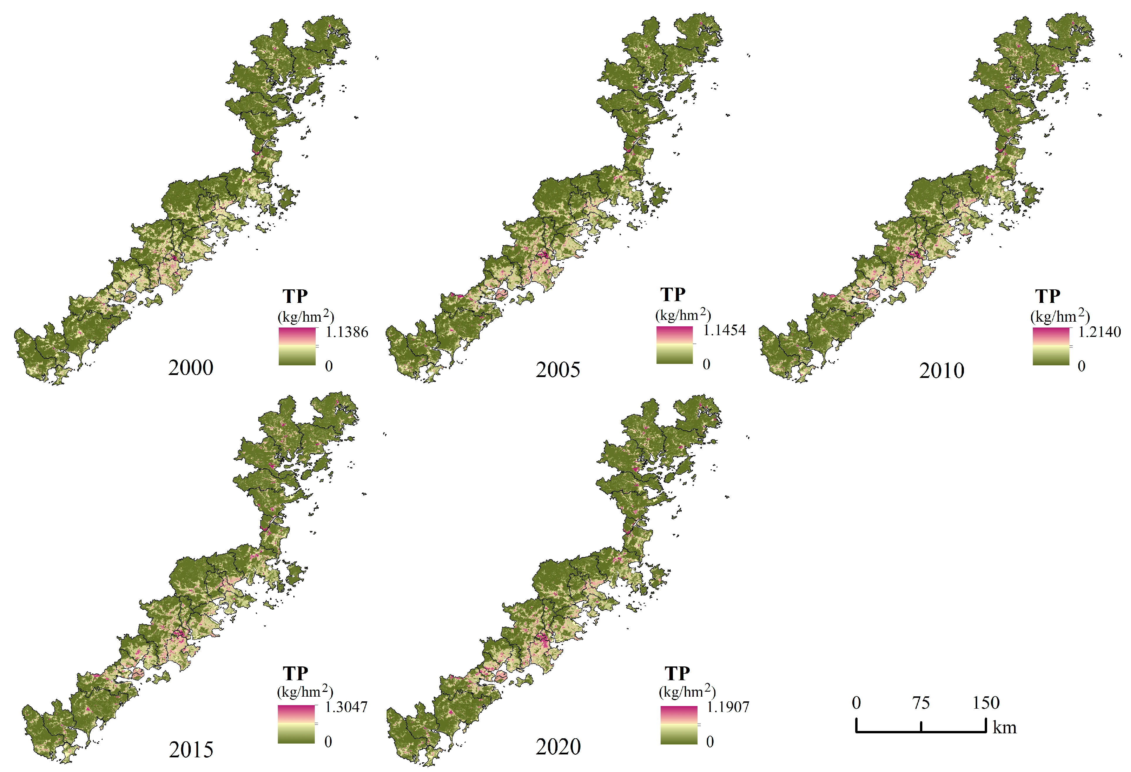
3.1.3. Nutrient Delivery Ratio
3.2. Ecological Security Barrier Function Index
3.3. Spatial Heterogeneity Analysis
3.4. Multiscale Geographically Weighted Regression (MGWR) Model
4. Results
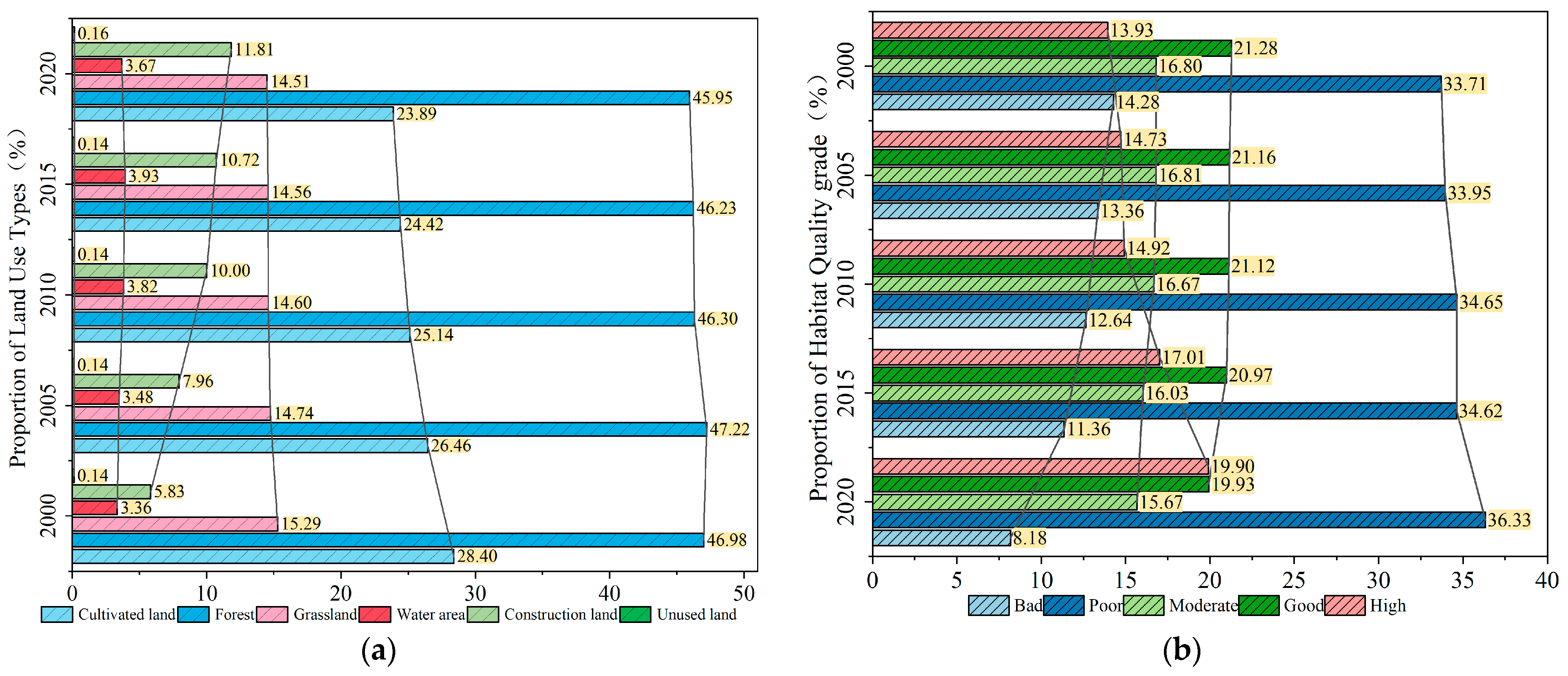
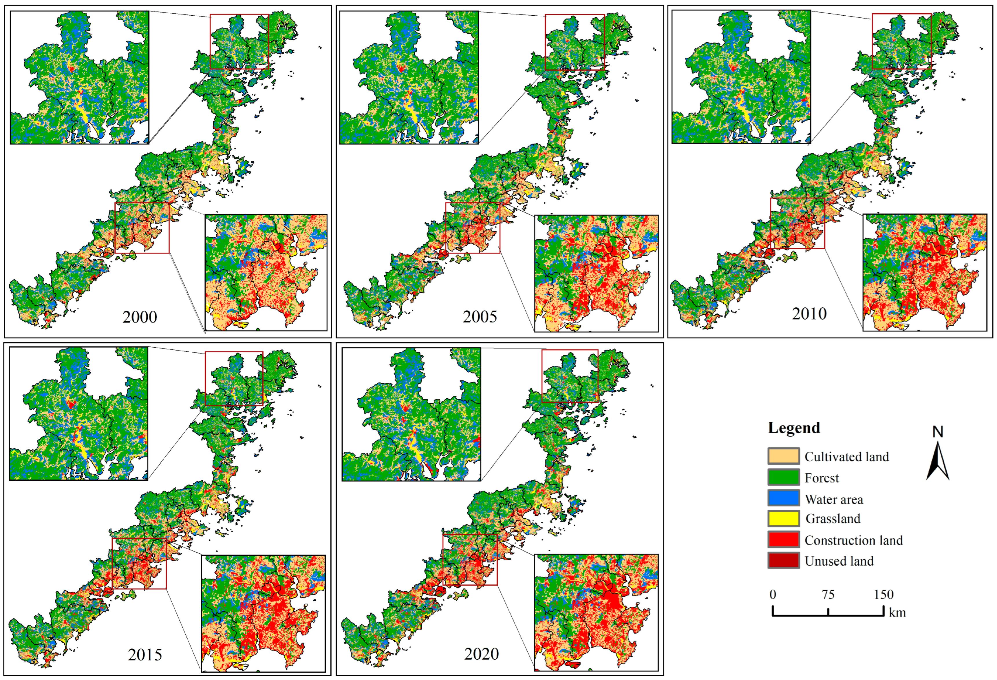
4.1. Dynamic Change of Land Use
4.2. Habitat Maintenance Services
4.3. Water Supply Service
4.4. Water Purification Service
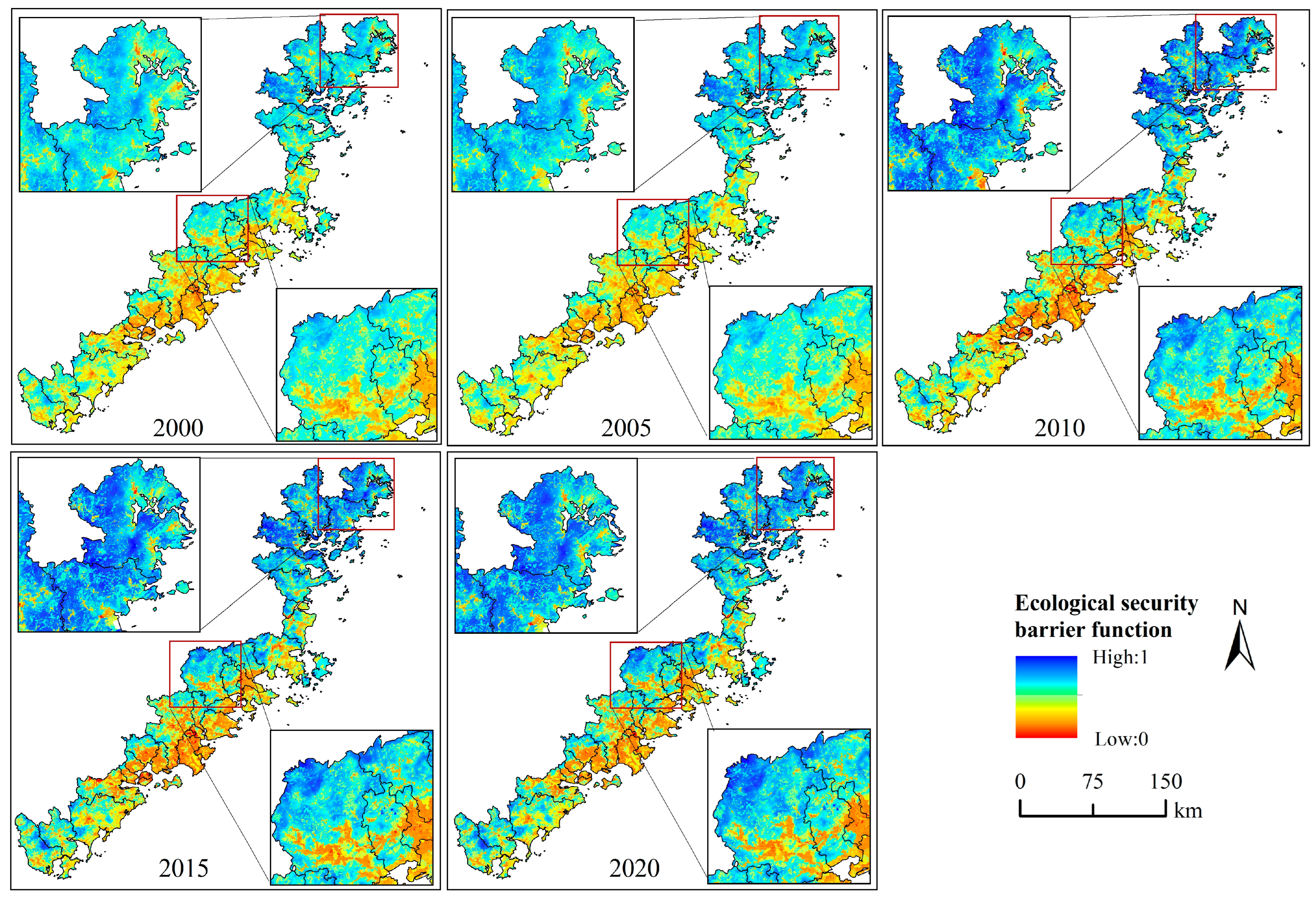
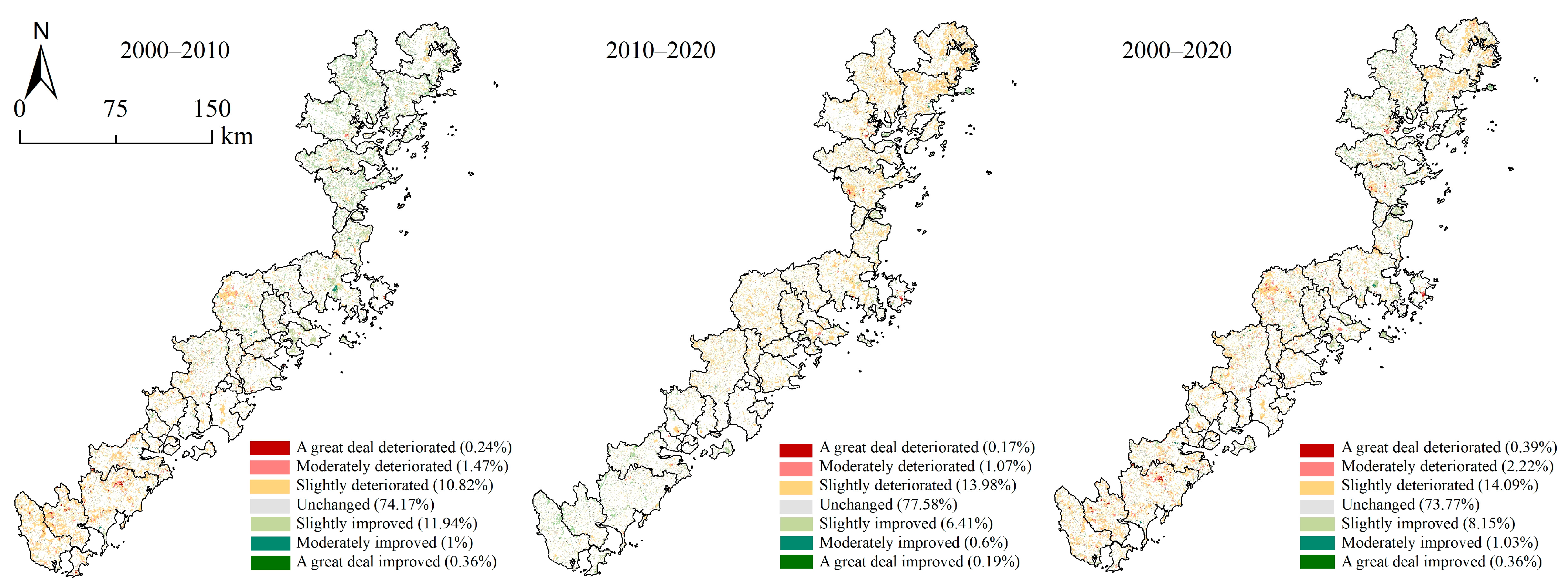
4.5. Dynamic Change Analysis of Ecological Safety Barrier Function (ESBF)
4.6. Analysis of the Driving Factors of ESBF
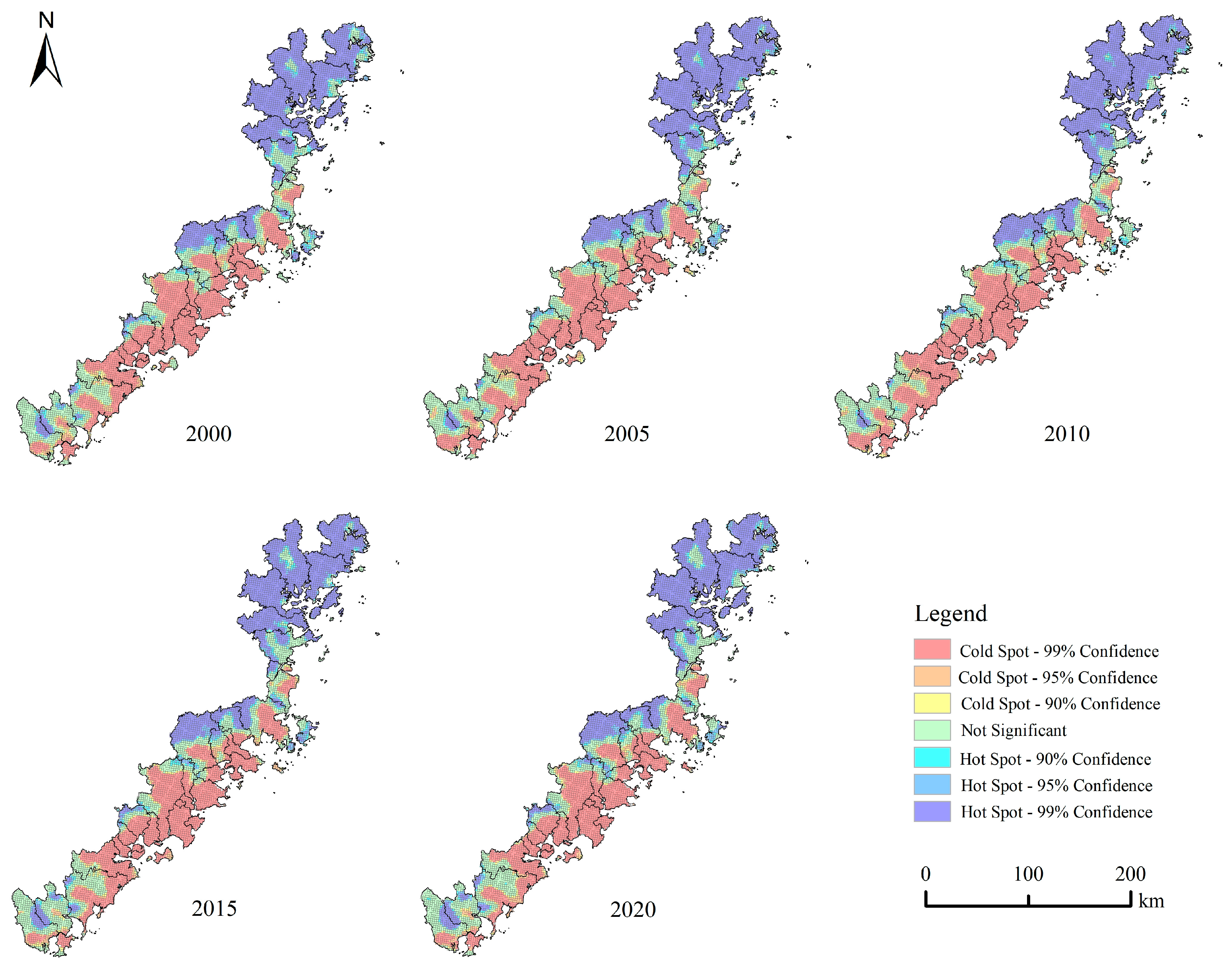
4.6.1. Spatial Autocorrelation Analysis
4.6.2. Analysis of Driving Factors Based on the MGWR Model
5. Discussion
5.1. Construction of Ecological Safety Barrier Function Index
5.2. Analysis of Driving Mechanism
5.3. Limitations
6. Conclusions
Author Contributions
Funding
Institutional Review Board Statement
Informed Consent Statement
Data Availability Statement
Acknowledgments
Conflicts of Interest
Abbreviations
| Acronym | Full Form |
| ESBF | Ecosystem Security Barrier Function |
| MGWR | Multiscale Geographically Weighted Regression |
| NDVI | Normalized Difference Vegetation Index |
| DEM | Digital Elevation Model |
| TN | Total Nitrogen |
| TP | Total Phosphorus |
| NDR | Nutrient Delivery Ratio |
| OLS | Ordinary Least Squares |
| AICc | Akaike Information Criterion, Corrected |
| Tol | Tolerance |
| VIF | Variance Inflation Factor |
References
- Hidalgo-Corrotea, C.; Alaniz, A.J.; Vergara, P.M.; Moreira-Arce, D.; Carvajal, M.A.; Pacheco-Cancino, P.; Espinosa, A. High Vulnerability of Coastal Wetlands in Chile at Multiple Scales Derived from Climate Change, Urbanization, and Exotic Forest Plantations. Sci. Total Environ. 2023, 903, 166130. [Google Scholar] [CrossRef] [PubMed]
- Ristić, V.; Trišić, I.; Štetić, S.; Maksin, M.; Nechita, F.; Candrea, A.N.; Pavlović, M.; Hertanu, A. Institutional, Ecological, Economic, and Socio-Cultural Sustainability—Evidence from Ponjavica Nature Park. Land 2024, 13, 669. [Google Scholar] [CrossRef]
- Wu, W.; Zhi, C.; Gao, Y.; Chen, C.; Chen, Z.; Su, H.; Lu, W.; Tian, B. Increasing Fragmentation and Squeezing of Coastal Wetlands: Status, Drivers, and Sustainable Protection from the Perspective of Remote Sensing. Sci. Total Environ. 2022, 811, 152339. [Google Scholar] [CrossRef] [PubMed]
- Gao, Y.; Liu, Z.; Li, R.; Shi, Z. Long-Term Impact of China’s Returning Farmland to Forest Program on Rural Economic Development. Sustainability 2020, 12, 1492. [Google Scholar] [CrossRef]
- Chinese Government Website. Available online: https://www.gov.cn/zhengce/zhengceku/2020-06/12/content_5518982.htm (accessed on 30 May 2024).
- Wang, X.; Yin, L.; Zhang, Y. Discussion on Several Issues Concerning Ecological Barriers. J. Ecol. Environ. 2016, 25, 2035–2040. [Google Scholar] [CrossRef]
- Wang, X.; Wang, X.; Zhang, X.; Zhou, J.; Jia, Z.; Ma, J.; Yao, W.; Tu, Y.; Sun, Z.; Wei, Y. Ecological Barriers: An Approach to Ecological Conservation and Restoration in China. Ambio 2024, 53, 1077–1091. [Google Scholar] [CrossRef] [PubMed]
- Tang, L.; Liang, G.; Gu, G.; Xu, J.; Duan, L.; Zhang, X.; Yang, X.; Lu, R. Study on the Spatial-Temporal Evolution Characteristics, Patterns, and Driving Mechanisms of Ecological Environment of the Ecological Security Barriers on China’s Land Borders. Environ. IMPACT Assess. Rev. 2023, 103, 107267. [Google Scholar] [CrossRef]
- Daily, G.C. Nature’s Services: Societal Dependence on Natural Ecosystems; Island Press: Washington, DC, USA, 1997. [Google Scholar]
- Costanza, R.; d’Arge, R.; de Groot, R.; Farber, S. The Value of the World’s Ecosystem Services and Natural Capital. Nature 1997, 387, 253–260. [Google Scholar] [CrossRef]
- Liang, S.; Yang, F.; Zhang, J.; Xiong, S.; Xu, Z. Assessment and Management Zoning of Ecosystem Service Trade-Off/Synergy Based on the Social–Ecological Balance: A Case of the Chang-Zhu-Tan Metropolitan Area. Land 2024, 13, 127. [Google Scholar] [CrossRef]
- Syrbe, R.-U.; Walz, U. Spatial Indicators for the Assessment of Ecosystem Services: Providing, Benefiting and Connecting Areas and Landscape Metrics. Ecol. Indic. 2012, 21, 80–88. [Google Scholar] [CrossRef]
- Lu, X.; Zheng, B.; Lian, Y.; Mo, X.; Li, H. Evaluation of Ecological Security Barrier Function in the Coastal Area of Bohai Bay: A Perspective of Ecosystem Service Supply and Demand. J. Saf. Environ. 2024, 24, 1200–1208. [Google Scholar] [CrossRef]
- Hasan, S.S.; Zhen, L.; Miah, M.G.; Ahamed, T.; Samie, A. Impact of Land Use Change on Ecosystem Services: A Review. Environ. Dev. 2020, 34, 100527. [Google Scholar] [CrossRef]
- Gao, J.; Li, F.; Gao, H.; Zhou, C.; Zhang, X. The Impact of Land-Use Change on Water-Related Ecosystem Services: A Study of the Guishui River Basin, Beijing, China. J. Clean. Prod. 2017, 163, S148–S155. [Google Scholar] [CrossRef]
- Wu, Z.; Chen, X.; Liu, B.; Chu, J.; Peng, L. Risk Assessment of Nitrogen and Phosphorus Nutrient Load Based on InVEST Model in Hainan Island. J. Trop. Crops 2013, 34, 1791–1797. [Google Scholar]
- Wang, B.; Cheng, W. Effects of Land Use/Cover on Regional Habitat Quality under Different Geomorphic Types Based on InVEST Model. Remote Sens. 2022, 14, 1279. [Google Scholar] [CrossRef]
- Hu, J.; Zhang, J.; Li, Y. Exploring the Spatial and Temporal Driving Mechanisms of Landscape Patterns on Habitat Quality in a City Undergoing Rapid Urbanization Based on GTWR and MGWR: The Case of Nanjing, China. Ecol. Indic. 2022, 143, 109333. [Google Scholar] [CrossRef]
- Zheng, Q.; Xu, G.; Liu, Y.; Yang, Q.; Chi, J.; Sun, J.; Zhang, T. Habitat Quality Assessment and Driving Forces in Anhui Province Based on InVEST and MGWR Models. Res. Soil Water Conserv. 2024, 31, 373–382. [Google Scholar] [CrossRef]
- Su, K.; Wei, D.; Lin, W. Evaluation of Ecosystem Services Value and Its Implications for Policy Making in China—A Case Study of Fujian Province. Ecol. Indic. 2020, 108, 105752. [Google Scholar] [CrossRef]
- Wang, Z.; Liu, Y.; Xie, X.; Wang, X.; Lin, H.; Xie, H.; Liu, X. Identifying Key Areas of Green Space for Ecological Restoration Based on Ecological Security Patterns in Fujian Province, China. Land 2022, 11, 1496. [Google Scholar] [CrossRef]
- Lu, C.; Lei, Y.; Su, Y.; Huang, Y.; Liu, M.; Jia, M. Remote sensing analysis of wetland dynamics in low-altitude coastal zone of southeast Fujian Province based on object-oriented and deep learning. Remote Sens. Technol. Appl. 2019, 36, 713–727. [Google Scholar]
- Wang, J.; Yan, Y.; Wang, J.; Ying, L.; Tang, Q. Study on the Temporal and Spatial Evolution Characteristics and Prediction of Habitat Quality in the Minjiang River Basin. Acta Ecol. Sin. 2021, 41, 5837–5848. [Google Scholar]
- Zhao, Y.; He, L.; Bai, W.; He, Z.; Luo, F.; Wang, Z. Prediction of Ecological Security Patterns Based on Urban Expansion: A Case Study of Chengdu. Ecol. Indic. 2024, 158, 111467. [Google Scholar] [CrossRef]
- Chen, X.; Chen, S.; He, Z.; Xue, D.; Fang, G.; Pan, K.; Fang, K. Developing a System for Comprehensive Regional Eco-Environmental Quality Assessment in Mountainous Areas—A Case Study of Western Sichuan, China. Front. Environ. Sci. 2022, 10, 879662. [Google Scholar] [CrossRef]
- Jia, Y.; Wang, S.; Liu, F.; Yu, D. Land Use Change and Its Correlation with Habitat Quality in the Efficient Ecological Economic Zone of the Yellow River Delta. Bull. Soil Water Conserv. 2020, 40, 213–220+227+330. [Google Scholar] [CrossRef]
- Zhao, Y.; Zhou, J. Identification of Driving Factors for Water Yield in the Upper Reaches of Shiyang River Based on InVEST Model. Chin. J. Ecol. 2019, 38, 3789. [Google Scholar]
- Li, M.; Li, S.; Liu, H.; Zhang, J. Balancing Water Ecosystem Services: Assessing Water Yield and Purification in Shanxi. Water 2023, 15, 3261. [Google Scholar] [CrossRef]
- Zhang, J.; Lei, G.; Qi, L. Landscape Pattern Change and Nitrogen and Phosphorus Purification Capacity in Danjiangkou City, Water Source Area of the Middle Route of the South-to-North Water Transfer Project. Acta Ecol. Sin. 2021, 41, 2261–2271. [Google Scholar]
- Liu, Y.; Lv, J.; Bi, J. Characterization and Driving Force Analysis of Water Purification Services in Terrestrial Ecosystems of Watersheds. Prog. Geogr. 2019, 38, 588–599. [Google Scholar]
- Chen, Z.; Lin, J.; Huang, J. Study on Freshwater Ecosystem Service Flow in Watersheds of Southeastern Fujian under Water Quality Stress. J. Ecol. Rural Environ. 2022, 38, 1051–1063. [Google Scholar] [CrossRef]
- Luo, F.; Pan, A.; Chen, Z.; Wang, Y. Spatial and Temporal Pattern Changes and Driving Factors of Cultivated Land in Yibin City, Sichuan Province from 1980 to 2018. Bull. Soil Water Conserv. 2021, 41, 336–344. [Google Scholar] [CrossRef]
- Zhu, W.; Lin, J.; Yang, S.; Chen, M.; Dai, Y.; Zhu, Y. Analysis of the Temporal and Spatial Evolution Characteristics and Influencing Factors of County-Level Forest Loss in Fujian Province. J. Ecol. Rural Environ. 2024, 40, 499–512. [Google Scholar] [CrossRef]
- Li, S.; Liu, J.; Lin, J.; Fan, S. Temporal and Spatial Evolution of Habitat Quality in Fujian Province Based on Land Use Change from 1980 to 2018. Chin. J. Appl. Ecol. 2020, 31, 4080–4090. [Google Scholar] [CrossRef]
- Hong, B.; Lin, Q.; Yu, S.; Zhang, D.; Yang, L. Spatial and Temporal Differentiation of the Impact Intensity of Human Activities and Economic Driving Mechanism in Coastal Wetlands of Fujian Province. J. Guilin Univ. Technol. 2019, 39, 678–684. [Google Scholar]
- Sallustio, L.; De Toni, A.; Strollo, A.; Di Febbraro, M.; Gissi, E.; Casella, L.; Geneletti, D.; Munafò, M.; Vizzarri, M.; Marchetti, M. Assessing Habitat Quality in Relation to the Spatial Distribution of Protected Areas in Italy. J. Environ. Manag. 2017, 201, 129–137. [Google Scholar] [CrossRef] [PubMed]
- Zeng, Y.; Li, C.; Huang, X.; Lin, H. Temporal and spatial variations of extreme precipitation in Fujian Province in recent 60 years. Soil Water Conserv. Res. 2023, 30, 203–210. [Google Scholar] [CrossRef]
- Wang, Q.; Ni, J.; Tenhunen, J. Application of a Geographically-Weighted Regression Analysis to Estimate Net Primary Production of Chinese Forest Ecosystems. Glob. Ecol. Biogeogr. 2005, 14, 379–393. [Google Scholar] [CrossRef]
- Wu, J.; Luo, J.; Zhang, H.; Qin, S.; Yu, M. Projections of Land Use Change and Habitat Quality Assessment by Coupling Climate Change and Development Patterns. Sci. Total Environ. 2022, 847, 157491. [Google Scholar] [CrossRef] [PubMed]
- Pei, H.; Liu, M.; Shen, Y.; Xu, K.; Zhang, H.; Li, Y.; Luo, J. Quantifying Impacts of Climate Dynamics and Land-Use Changes on Water Yield Service in the Agro-Pastoral Ecotone of Northern China. Sci. Total Environ. 2022, 809, 151153. [Google Scholar] [CrossRef] [PubMed]
- Yu, H.; Yang, J.; Qiu, M.; Liu, Z. Spatiotemporal Changes and Obstacle Factors of Forest Ecological Security in China: A Provincial-Level Analysis. Forests 2021, 12, 1526. [Google Scholar] [CrossRef]
- Li, Z.; Zuo, X.; Teng, J. Temporal and Spatial Variation Pattern of Red Tides in China’s Coastal Waters from 1950 to 2020 Based on GIS. Acta Sci. Circumstantiae 2023, 43, 203–214. [Google Scholar] [CrossRef]
- Huang, C.; Zhao, D.; Liao, Q.; Xiao, M. Linking Landscape Dynamics to the Relationship between Water Purification and Soil Retention. Ecosyst. Serv. 2023, 59, 101498. [Google Scholar] [CrossRef]
- Zou, L.; Liu, Y.; Wang, Y.; Hu, X. Assessment and Analysis of Agricultural Non-Point Source Pollution Loads in China: 1978–2017. J. Environ. Manag. 2020, 263, 110400. [Google Scholar] [CrossRef] [PubMed]
- Lai, X.; Zeng, C.; Su, Y.; Huang, S.; Jia, J.; Chen, C.; Jiang, J. Vulnerability Assessment of Coastal Wetlands in Minjiang River Estuary Based on Cloud Model under Sea Level Rise. Acta Oceanol. Sin. 2023, 42, 160–174. [Google Scholar] [CrossRef]
- Liu, Q.; Zhao, E.; Wang, K.; Xiong, X.; Wu, C. Analysis of Water Environment Characteristics and Water Purification Capacity of Natural Wetlands on the Qinghai-Tibet Plateau. J. Hydrobiol. 2022, 46, 1797–1806. [Google Scholar]
- Geng, A.; Yang, Z.; Li, Y.; Kang, W.; Gao, J.; Li, Q.; Gao, J. Design of Combined Artificial Wetlands with Both Water Purification and Regulation Functions. China Water Wastewater 2023, 39, 59–64. [Google Scholar] [CrossRef]
- Yu, Q.; Feng, C.-C.; Shi, Y.; Guo, L. Spatiotemporal Interaction between Ecosystem Services and Urbanization in China: Incorporating the Scarcity Effects. J. Clean. Prod. 2021, 317, 128392. [Google Scholar] [CrossRef]
- Vicente-Serrano, S.M.; Quiring, S.M.; Peña-Gallardo, M.; Yuan, S.; Domínguez-Castro, F. A Review of Environmental Droughts: Increased Risk under Global Warming? Earth-Sci. Rev. 2020, 201, 102953. [Google Scholar] [CrossRef]
- Zhong, F.; Xu, X.; Li, Z.; Zeng, X.; Yi, R.; Luo, W.; Zhang, Y.; Xu, C. Relationships between Lithology, Topography, Soil, and Vegetation, and Their Implications for Karst Vegetation Restoration. CATENA 2022, 209, 105831. [Google Scholar] [CrossRef]
- Yin, L.; Feng, X.; Fu, B.; Wang, S.; Wang, X.; Chen, Y.; Tao, F.; Hu, J. A Coupled Human-Natural System Analysis of Water Yield in the Yellow River Basin, China. Sci. Total Environ. 2021, 762, 143141. [Google Scholar] [CrossRef]
- Müller, A.; Olschewski, R.; Unterberger, C.; Knoke, T. The Valuation of Forest Ecosystem Services as a Tool for Management Planning—A Choice Experiment. J. Environ. Manag. 2020, 271, 111008. [Google Scholar] [CrossRef]
- Zhang, Y.; Wu, T.; Arkema, K.K.; Han, B.; Lu, F.; Ruckelshaus, M.; Ouyang, Z. Coastal Vulnerability to Climate Change in China’s Bohai Economic Rim. Environ. Int. 2021, 147, 106359. [Google Scholar] [CrossRef] [PubMed]
- Levin, N.; Kyba, C.C.M.; Zhang, Q.; Sánchez de Miguel, A.; Román, M.O.; Li, X.; Portnov, B.A.; Molthan, A.L.; Jechow, A.; Miller, S.D.; et al. Remote Sensing of Night Lights: A Review and an Outlook for the Future. Remote Sens. Environ. 2020, 237, 111443. [Google Scholar] [CrossRef]


| Data | Data Resources | Description |
|---|---|---|
| Land Use Dataset | Resource and Environment Science and Data Center (https://www.resdc.cn) (accessed on 4 February 2024). | Raster, 30 m × 30 m |
| Population Spatial Distribution | Raster, 1 km × 1 km | |
| Watershed | shapefile | |
| River Network | shapefile | |
| Annual Mean Precipitation | Raster, 1 km × 1 km | |
| Annual Mean Temperature | Raster, 1 km × 1 km | |
| Soil type | Raster, 30 m × 30 m | |
| Soil clay content | Raster, 1 km × 1 km | |
| Soil organic carbon content | Raster, 1 km × 1 km | |
| Nighttime Light Data | Harvard Dataverse (https://dataverse.harvard.edu/dataverse/harvard/?q=nighttime+light) (accessed on 12 February 2024). | Raster, 30 arc s |
| DEM (Digital Elevation Model) | Geospatial Data Cloud (https://www.gscloud.cn/) (accessed on 12 February 2024). | Raster, 30 m × 30 m |
| NDVI (Normalized Difference Vegetation Index) | NASA LP DAAC at the USGS EROS Center (https://lpdaac.usgs.gov/products/mod13a1v006/) (accessed on 12 February 2024). | Raster, 500 m × 500 m |
| Evapotranspiration Data | https://doi.org/10.5194/essd-11-1931-2019 (accessed on 13 February 2024). | Raster, 1 km × 1 km |
| China Bedrock Depth Dataset | http://globalchange.bnu.edu.cn/research/cdtb.jsp (accessed on 13 February 2024). | Raster, 100 m × 100 m |
| Available Water Capacity (SoilGrids 2017 AWC) | https://data.isric.org/geonetwork/srv/eng/catalog.search#/metadata/e33e75c0-d9ab-46b5-a915-cb344345099c (accessed on 14 February 2024). | Raster, 250 m × 250 m |
| Threat | Max_dist | Weight | Decay |
|---|---|---|---|
| Dry Land | 3 | 0.6 | Linear |
| Urban Land | 5 | 0.7 | Exponential |
| Paddy Field | 3 | 0.6 | Linear |
| Other Building Land | 6 | 0.9 | Exponential |
| Rural Settlements | 10 | 1 | Exponential |
| Land Use Types | HABITAT | Paddy Field | Dryland | Urban Land | Rural Settlements | Other Building Land |
|---|---|---|---|---|---|---|
| No Data | 0 | 0 | 0 | 0 | 0 | 0 |
| Paddy Field | 0.4 | 0.3 | 0.3 | 0.5 | 0.4 | 0.5 |
| Dry Land | 0.4 | 0.3 | 0.3 | 0.5 | 0.4 | 0.5 |
| Forested land | 1 | 0.8 | 0.8 | 0.9 | 0.8 | 0.8 |
| Shrubland | 0.8 | 0.4 | 0.4 | 0.8 | 0.7 | 0.7 |
| Open woodland | 0.6 | 0.85 | 0.85 | 0.9 | 0.8 | 0.8 |
| Other woodland | 0.4 | 0.9 | 0.9 | 0.9 | 0.8 | 0.8 |
| High Cover Grassland | 0.7 | 0.4 | 0.4 | 0.6 | 0.5 | 0.6 |
| Medium Cover Grassland | 0.5 | 0.45 | 0.45 | 0.65 | 0.55 | 0.65 |
| Low Cover Grassland | 0.3 | 0.5 | 0.5 | 0.7 | 0.6 | 0.7 |
| Rivers | 0.9 | 0.65 | 0.65 | 0.85 | 0.75 | 0.8 |
| Lakes | 1 | 0.7 | 0.7 | 0.9 | 0.8 | 0.7 |
| Reservoirs and Ponds | 0.8 | 0.7 | 0.7 | 0.9 | 0.8 | 0.7 |
| Mudflat | 0.6 | 0.75 | 0.75 | 0.95 | 0.85 | 0.7 |
| Beaches | 0.6 | 0.75 | 0.75 | 0.95 | 0.85 | 0.7 |
| Urban Land | 0 | 0 | 0 | 0 | 0 | 0 |
| Rural Settlements | 0 | 0 | 0 | 0 | 0 | 0 |
| Other Building Land | 0 | 0 | 0 | 0 | 0 | 0 |
| Marshland | 0.9 | 0.7 | 0.7 | 0.8 | 0.75 | 0.6 |
| Bare Land | 0 | 0 | 0 | 0 | 0 | 0 |
| Rocky Land | 0 | 0 | 0 | 0 | 0 | 0 |
| Ocean | 0 | 0 | 0 | 0 | 0 | 0 |
| Landuse Types | Load_p * | eff_p * | Crit_len_p * | Load_n * | eff_n * | crit_len_n * |
|---|---|---|---|---|---|---|
| Cultivated land | 1.22 | 0.35 | 25 | 19.4 | 0.25 | 25 |
| Forest land | 0.15 | 0.8 | 300 | 2.12 | 0.72 | 300 |
| Grassland | 0.2 | 0.48 | 150 | 3.2 | 0.4 | 150 |
| Water area | 0.01 | 0.05 | 150 | 0.01 | 0.05 | 150 |
| Construction land | 2.1 | 0.05 | 10 | 12 | 0.05 | 10 |
| Unuseed land | 0.05 | 0.05 | 150 | 1.45 | 0.05 | 10 |
| Parameters | Collinearity Diagnostics | MGWR (Bandwidth: 71–8107) | GWR (Bandwidth: 295) | Globle OLS | |||||
|---|---|---|---|---|---|---|---|---|---|
| Tol | VIF | Min | Mean | Max | Min | Mean | Max | ||
| Temperature | 0.25 | 3.94 | −0.16 | −0.02 | 0.20 | −0.56 | −0.05 | 0.45 | −0.12 |
| Precipitation | 0.40 | 2.51 | 0.04 | 0.31 | 1.02 | −0.20 | 0.34 | 1.76 | 0.31 |
| Population | 0.77 | 1.30 | −0.31 | −0.07 | 0.12 | −0.89 | −0.06 | 0.79 | −0.01 |
| NDVI | 0.38 | 2.66 | −0.13 | 0.22 | 0.72 | −0.35 | 0.04 | 0.57 | 0.02 |
| Night time light | 0.47 | 2.15 | −1.34 | −0.17 | 0.20 | −1.31 | −0.15 | 1.42 | −0.09 |
| Construction Land Ratio | 0.42 | 2.37 | −0.40 | −0.15 | 0.01 | −1.15 | −0.16 | 0.22 | −0.14 |
| Cultivated Land Ratio | 0.68 | 1.48 | −0.61 | −0.28 | −0.04 | −0.62 | −0.29 | −0.07 | −0.31 |
| Slope | 0.60 | 1.67 | 0.11 | 0.16 | 0.20 | −0.16 | 0.07 | 0.33 | 0.07 |
| Elevation | 0.45 | 2.23 | −0.25 | 0.14 | 0.33 | −0.22 | 0.18 | 1.00 | 0.11 |
| Soil Clay Content | 0.96 | 1.04 | −0.09 | 0.03 | 0.21 | −0.17 | 0.03 | 0.43 | 0.03 |
| Soil Organic Carbon Content | 0.73 | 1.37 | −0.32 | −0.02 | 0.12 | −0.45 | −0.03 | 0.20 | −0.05 |
| R2 | - | - | 0.758 | - | - | 0.769 | - | - | 0.691 |
| Adjusted R2 | - | - | 0.744 | - | - | 0.750 | - | - | 0.690 |
| AICc | - | - | 12,454 | - | - | 12,503 | - | - | 13,240 |
Disclaimer/Publisher’s Note: The statements, opinions and data contained in all publications are solely those of the individual author(s) and contributor(s) and not of MDPI and/or the editor(s). MDPI and/or the editor(s) disclaim responsibility for any injury to people or property resulting from any ideas, methods, instructions or products referred to in the content. |
© 2024 by the authors. Licensee MDPI, Basel, Switzerland. This article is an open access article distributed under the terms and conditions of the Creative Commons Attribution (CC BY) license (https://creativecommons.org/licenses/by/4.0/).
Share and Cite
Luo, F.; He, L.; He, Z.; Zeng, W.; Wang, Y. Evaluation of Coastal Ecological Security Barrier Functions Based on Ecosystem Services: A Case Study of Fujian Province, China. Sustainability 2024, 16, 6787. https://doi.org/10.3390/su16166787
Luo F, He L, He Z, Zeng W, Wang Y. Evaluation of Coastal Ecological Security Barrier Functions Based on Ecosystem Services: A Case Study of Fujian Province, China. Sustainability. 2024; 16(16):6787. https://doi.org/10.3390/su16166787
Chicago/Turabian StyleLuo, Fang, Li He, Zhengwei He, Wanting Zeng, and Yuanchao Wang. 2024. "Evaluation of Coastal Ecological Security Barrier Functions Based on Ecosystem Services: A Case Study of Fujian Province, China" Sustainability 16, no. 16: 6787. https://doi.org/10.3390/su16166787
APA StyleLuo, F., He, L., He, Z., Zeng, W., & Wang, Y. (2024). Evaluation of Coastal Ecological Security Barrier Functions Based on Ecosystem Services: A Case Study of Fujian Province, China. Sustainability, 16(16), 6787. https://doi.org/10.3390/su16166787