Modeling of Soil Cation Exchange Capacity Based on Chemometrics, Various Spectral Transformations, and Multivariate Approaches in Some Soils of Arid Zones

Abstract

Cation exchange capacity is a crucial metric for managing soil fertility and promoting agricultural sustainability. An alternative technique for the non-destructive assessment of important soil parameters is reflectance spectroscopy. The main focus of this paper is on how to analyze and predict the content of various soil cation exchange capacities (CEC) in arid conditions (Sohag governorate, Egypt) at a low cost using laboratory analysis of CEC, visible near-infrared and shortwave infrared (Vis-NIR) spectroscopy, partial least-squares regression (PLSR), and Ordinary Kriging (OK). Utilizing reflectance spectroscopy with a spectral resolution of 10 nm and laboratory studies with a spectral range of 350 to 2500 nm, 104 surface soil samples were collected to a depth of 30 cm in the Sohag governorate, Egypt (which is part of the dry region of North Africa), in order to accomplish this goal. The association between the spectroradiometer and CEC averaged values was modeled using PLSR in order to map the predicted value using Ordinary Kriging (OK). Thirty-one soil samples were selected for validation. The predictive validity of the cross-validated models was evaluated using the coefficient of determination (R²), root mean square error (RMSE), residual prediction deviation (RPD), and ratio of performance to interquartile distance (RPIQ). The results indicate that ten transformation methods yielded calibration models that met the study’s requirements, with R² > 0.6, RPQ > 2.5, and RIQP > 4.05. For evaluating CEC in Vis-NIR spectra, the most efficient transformation and calibration model was the reciprocal of Log R transformation (R² = 0.98, RMSE = 0.40, RPD = 6.99, and RIQP = 9.22). This implies that combining the reciprocal of Log R with PLSR yields the optimal model for predicting CEC values. The CEC values were best fitted by four models: spherical, exponential, Gaussian, and circular. The methodology used here does offer a “quick”, inexpensive tool that can be broadly and quickly used, and it can be readily implemented again in comparable conditions in arid regions.

1. Introduction

Managing soil fertility and advancing agricultural sustainability require a measurement known as cation exchange capacity (CEC). Traditionally, components such as fertility have been determined through laboratory soil analysis. This is time-consuming and expensive, which raises concerns for precision agriculture’s future, which has stalled in several nations [1]. The ability of soil to adsorb and exchange cations is known as its cation exchange capacity (CEC). Furthermore, CEC is a crucial measure for mineralogical characterization and soil fertility [2,3]. One of the primary chemical characteristics of soil is its cation exchange capacity (CEC), which is necessary for several disciplines, including soil science, agricultural and environmental engineering, and soil science [4].

For the determination of CEC, a number of traditional laboratory analysis techniques have historically been available [5]. According to Richards [6] the majority of procedures entail saturating the soil with an index cation (NH₄), eliminating surplus cations by washing, replacing the adsorbed index cation with another cation (Na), and measuring the index cation in the final extract. Furthermore, due to increased Ca solubility in calcareous and gypsiferous soils, new approaches have been implemented [7]. However, the current methods are costly, labor-intensive, and time-consuming, especially when dealing with a lot of soil samples [8,9]. The scientific community is now working to provide quick and affordable ways for evaluating particular factors because of the difficulties involved with the traditional approaches. Although there has been significant advancement in the accurate application of machine learning algorithms for CEC prediction, these algorithms have not yet been applied to a variety of land uses worldwide [10].

One of the most promising methods for making fast decisions on soil qualities is chemometric analysis, which makes use of the visible, near-infrared, and shortwave infrared reflectance domains to predict different soil parameters. Vis-NIR spectroscopy has been shown in several studies to be useful for estimating soil properties, including CEC [11,12,13]. Through the use of Vis-NIR spectra, information is mostly connected to the organic matter (OM) content, water content, and mineral elements of the soil, such as clay minerals [14]. This information is encoded in the spectrum by its absorptions (spectral characteristics) at particular wavelengths, intensities, and shapes [15]. Additionally, the Vis-NIR approach enables the calculation of secondary soil parameters, or characteristics like pH, cation exchange capacity (CEC), base saturation (V), and exchangeable (ex-) nutrients that have indirect correlations with the spectrum [16]. When primary and secondary soil properties covariate, this is achievable [17]. The method’s ability to complete quick, non-destructive analysis with little to no sample preparation has led to its increasing use. It overcomes the drawbacks of wet chemistry by offering a chemical-free, real-time evaluation of soil quality that may be applied directly at a field location. In reaction to an infrared (IR) source, it creates a fingerprint of the sample that is closely related to its physicochemical makeup [18]. The rapid predictability of this technique when combined with statistical multivariate modeling makes it a viable alternative that has gained popularity for a number of nutrients, including soil organic carbon, nitrogen, phosphorus, potassium, and other nutrients [19,20,21].

The partial least-squares regression (PLSR) technique is the most well-known and extensively utilized multivariate statistical technique in chemometric research, with researchers worldwide using it [22]. PLSR is very useful when there is multicollinearity among predictors (X variables) and when the predictor matrix has many more variables than the number of observations. Because of its greater understandability and faster processing algorithm, PLSR is typically chosen over other multivariate statistical techniques [23]. Numerous researchers, such as Mousavi et al. [24] and Yitagesu et al. [25], have revealed that the primary benefit of PLSR is its great efficiency when dealing with small sample sizes.

Soil spectral data have been preprocessed using a variety of techniques to highlight characteristics, reduce noise, and prepare them for estimation modeling. For example, to find the optimal combination for estimating soil carbon, ref. [26] employed five multivariate approaches and thirty preprocessing transformations, such as derivatives, normalization, and non-linear transformations. The best performance, according to the authors, was shown by PLSR, which was followed by stepwise multiple linear regression (SMLR). Among the preprocessing adjustments, Savitzky–Golay derivatives often improved models for all multivariate approaches. Additionally, five machine learning (ML) model predictions and spatial uncertainties were developed and thoroughly assessed from the standpoint of a soil scientist by Kaya et al. [27]. Higher R² (0.41) values and lower RMSE (4.12 cmolc kg⁻¹) and MAE (3.12 cmolc kg⁻¹) values showed that the RF model performed better than the other models. Several artificial intelligence (AI) methods were employed by other studies to predict CEC [28,29]. Today, visible near-infrared and shortwave infrared (Vis-NIR) approaches are generally acknowledged to be useful for quantitatively retrieving soil parameters and typically yield good indicators of soil quality [30]. However, a number of important issues remain to be resolved, including the proportion of gypsum and carbonate, which is still a contentious subject today. Appropriate multivariate regression techniques, which have an advantage over some bivariate associations and are appropriate for peak intensity data, can be used to obtain quantitative information about CEC. Additionally, a variety of multivariate methods such as main components regression, multiple linear regression, and partial least squares stepwise linear regression (PLSR) support vector machines and multivariate adaptive regression splines can be utilized for several kinds of titrated soil examination [31]. With all of the above-mentioned details in mind, the current study set out to create predictive modeling of soil CEC in arid conditions (Sohag governorate, Egypt) utilizing a variety of spectral transformations and the PLSR approach.

2. Materials and Methods

2.1. Experimental Area

The study area covers a part (alluvial plain about 2021.1 km²) of Sohag governorate, Egypt, which extends from the northern edge of Qena Governorate at latitude 26°07′ N to the southern edge of Assiut Governorate at latitude 26°57′ N. It is bounded between longitudes 31°20′ and 32°14′ E with elevation varying from about 62 to 75 m above the mean sea level (Figure 1). The study area belongs to the arid region of North Africa, which is generally characterized by hot summers and mild winters with low rainfall. Air temperature ranges between 36.5 °C (summer) and 15.5 °C (winter), relative humidity ranges between 51% and 61% (winter), 33% and 41% (spring), and 35% and 42% (summer) ([32], Rainfall is generally rare and randomly precipitates over the area. The Nile River, irrigation canals, and drainage systems hydrologically reflect the surface water in the Sohag region. The Nile’s alluvial deposits created the Quaternary aquifer system in the research region, which is divided into two strata with different hydraulic characteristics. The clay–silt component, which is the top layer, has little permeability both vertically and horizontally. The primary aquifer with high horizontal and vertical permeability is formed by the lowest layer, the graded sand member [33].

2.2. Field Work and Lab Analysis

A total of 104 representative sites were chosen to encompass the study region (Figure 2). A hand-held GPS (Germin e-trix, Nevada, KS, USA) was used to record the location coordinates using the WGS 84 coordinate system. The sampling sites were chosen based on the spatial heterogeneity seen in the alluvial plain. A random sampling method was utilized. This entailed taking soil samples at random sites throughout the selected sampling region. Each soil sample was taken at each sampling location from three to five disturbed subsamples in the surface layer (0 to 30 cm); the soils were then combined and put into polyethylene bags for additional examination. The soil samples were allowed to air dry at room temperature; consequently, the dried soil samples were crushed using a wooden mortar and then sieved through a 2 mm sieve. The salinity (electric conductivity) with an EC meter (Orion, Model 150, Bosque Farms, NM, USA) [34], soil acidity (pH) in a saturated paste with a pH meter supplied from HANNA Instruments (Leighton Buzzard, UK) [35], and cation exchange capacity (CEC) [36] were measured. Furthermore, in accordance with [37], the particle size distribution was measured.

2.3. Acquisition of Spectral Data

A spectroradiometer FieldSpec 3 (ASD-Analytical Spectral Devices, Boulder, CO, USA) with a spectral range of 350 to 2500 nm and a spectral resolution of 10 nm, with a sampling interval of 1 nm, was used to collect the Vis-NIR laboratory-based spectral measurements under standard illumination conditions using two calibrated tungsten quartz halogen lamps in the dark. Petri dishes with roughly 95 cm³ of soil were filled with soil samples. For every soil sample, the equipment calculated an average of 100 scans. The spectroradiometer was calibrated using a white Spectralon with 100% reflectance (LabSphere, North Sutton, NH, USA) prior to scanning [38].

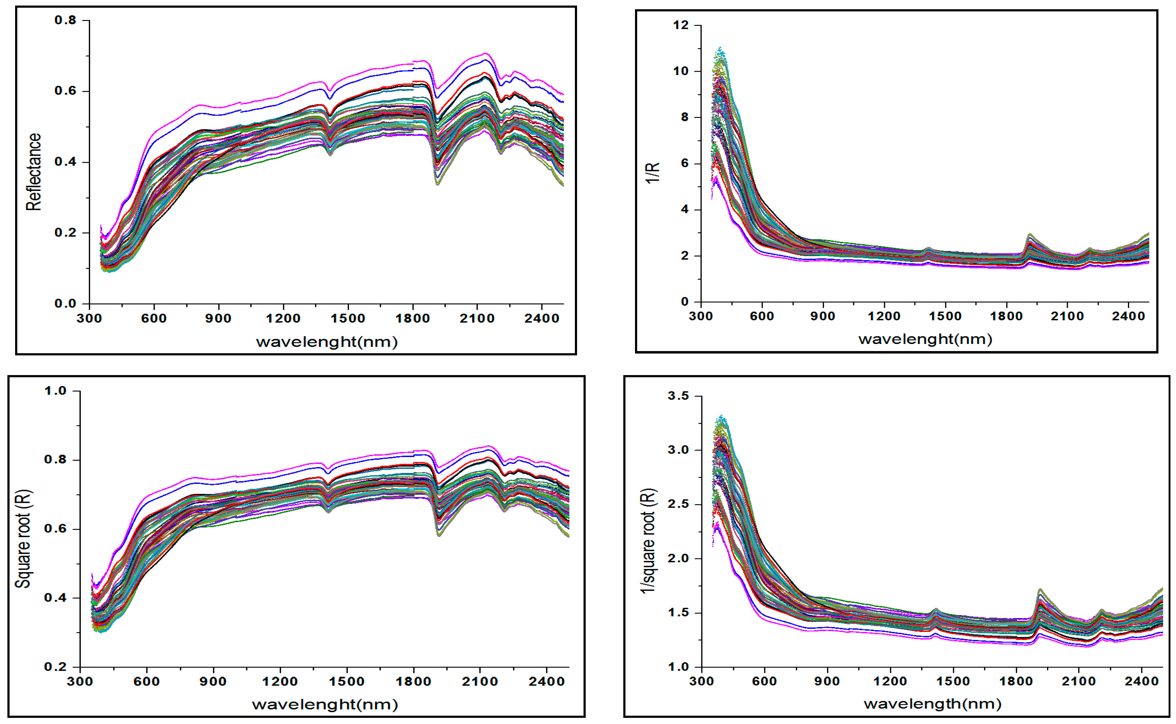
2.4. Data Preparation and Preprocessing Transformation

Utilizing a moving Savitzky–Golay filter algorithm [39] with a window width of 5 nm and a second-degree polynomial, the instrument noise was eliminated. The number of predictor variables in the soil Vis-NIR spectra was lowered from 2150 to 1075 by first averaging the data over two bands. This shortened the dataset’s dimensionality, slashed processing time, and made them ready for additional preparation. Preprocessing is often the first step in spectroscopic analysis, with the goal of assessing and potentially improving data quality. The spectral preprocessing method uses many mathematical strategies to improve the data and rectify light scattering in reflectance measurements before using the data in calibration models [40]. A comprehensive literature review was used to identify several reflectance transformations that are responsive to diverse soil conditions in the current investigation. The authors of [22,23,41,42] have provided a full description of the development of various reflectance transformations and their usage in the quantitative modeling of various soil parameters. In the current investigation, 18 distinct reflectance transformations were identified based on all of those studies, and their potential for quantitative CEC prediction was assessed using these transformations, i.e., Reflectance (R), Logarithm of R (Log R), Square root of R (√R), Reciprocal of R (1/R), Reciprocal of Log R (1/Log R), Reciprocal of √R (1/√R), First derivative of R (R’), First derivative of Log R (Log R)’, First derivative of √R→ (√R)’, Second derivative of R (R”), Second derivative of Log R (Log R)”, Second derivative of √R (√R)”, First derivative of 1/R (1/R)’, First derivative of 1/Log R (1/Log R)’, First derivative of 1/√R→ (1/√R)’, Second derivative of 1/R (1/R)”, Second derivative of 1/Log R (1/Log R)”→, and Second derivative of 1/√R (1/√R)”. The production of reflectance changes was performed using the spectral libraries that were created for each sample. Various reflectance value transformations help with hyperspectral modeling for the prediction of soil properties by eliminating noise (linear, linear-like, and multiplication noise), eliminating the additive baseline (or “offset”), and linearizing the previously non-linear correlation between measured reflectance and soil physico-chemical properties [23].

2.5. Multiple Variable Statistical Modeling

Using a variety of reflectance modifications, the Partial Least Square Regression (PLSR) technique was employed to predict soil attributes among the many multivariate statistical methods available for chemometric analysis. A popular Vis-NIR calibration method noted for its predictability, simplicity, accuracy, and quantitative explanations is called PLSR [43,44]. In general, PLSR is preferred due to its faster computational speed and easier-to-understand algorithm. Essentially, PLSR looks for a small number of components or factors (linear combinations) within the spectral data (original X values) and uses them to create regression equations that predict the observed variable (soil properties). Using laboratory soil data, Vis-NIR spectral data, the R studio software 4.1.2 PLS package was used to create the various soil parameters’ calibration and validation models in accordance with the protocol provided by [45]. The orthogonal components that increase the variance of the predictor (X spectra that are mean-centered before decomposition) and response variables (Y lab data from the chemical analysis) are chosen using the PLSR algorithm. Factor loading (P and q) and factor scores (T) are the breakdowns of X and Y provided by PLSR. Equations (1) and (2) include residues E and F to account for the remaining noise elements that can be ignored.

$$X=TP+E$$

(1)

$$Y=Tq+F$$

(2)

The entire dataset of 104 observations was randomly divided into two groups in order to determine the accuracy of the PLSR regression models: the validation dataset, which included 31 samples (30% of the total dataset), was used to test the developed model’s accuracy, and the calibration dataset, which included 73 samples (70% of the total dataset), for the development of the prediction model. To evaluate each PLSR component’s predictive importance, random cross-validation was used.

2.6. Assessment of the Developed Models’ Performance

The coefficient of determination (R²), root mean square error (RMSE), residual prediction deviation (RPD), and ratio of performance to interquartile distance (RPIQ) were used to assess the cross-validated models’ predictive quality as given in Equations (3)–(6).

$$R^2=n-\left({\displaystyle \frac{\sum {\left(Y_{Pred}-Y_{Meas}\right)}^2}{\sum {\left(Y_i-Y_{Meas}\right)}^2}}\right)$$

(3)

where Y_Pred is the soil predicted values; Yi is the soil measured values mean; Y_Meas is the soil measured values; and n is the number of measured or predicted values.

𝑅𝑀𝑆𝐸 = 1(𝑌 −𝑋)²

(4)

where Y is the soil predicted values; X is the soil measured values; and n is the number of measured or predicted values.

$$RPD={\displaystyle \frac{SD}{RMSE}}$$

(5)

where SD is the standard deviation.

The ratio of performance to IQ (RPIQ) value is more objective than the RPD value; however, Bellon-Maurel noted that both the chemical content and the physical characteristics of the soil show a biased normal distribution [46].

𝑅𝑃𝐼𝑄 = 𝐼𝑄𝑅𝑀𝑆𝐸 = 𝑄3 − 𝑄1𝑅𝑀𝑆𝐸

(6)

where:

The difference between the first quartile (Q1) and the third quartile (Q3), which is where we find 75% of the samples, is known as IQ. Q1 is the value below which we can find 25% of the samples.

Regression models of the spectrum have been extensively trained using these methods [47].

The best cross-validated models were those with the lowest RMSE and highest R², RPD, and RPIQ values. The validation dataset was later used to independently test the selected models, and R², RPD, RPIQ, and RMSE values were used to assess the overall prediction accuracy [23]. According to [48], the R² value indicated whether the model was: (1) fairly predicted (R²: 0.50–0.75); (2) unreliable (R² < 0.50); or (3) well suited to predict the attribute reliably (R² > 0.75). According to the values of (RPD), six categories of models/predictions were defined [44] as shown in (

Table 1. Interpretations of RPD values.

RPD	Interpretation
<1.0	Very poor
1.0–1.4	Poor
1.4–1.8	Fair
1.8–2.0	Good
2.0–2.5	Very good
>2.5	Excellent

).

Whereas, four classes of models were recognized based on RPIQ values [46] and presented in (

Table 2. Interpretations of RPIQ values.

RPIQ	Interpretation
2.02–2.7	Poor
2.7–3.37	Fair
3.27–4.05	Good
>4.05	Excellent

).

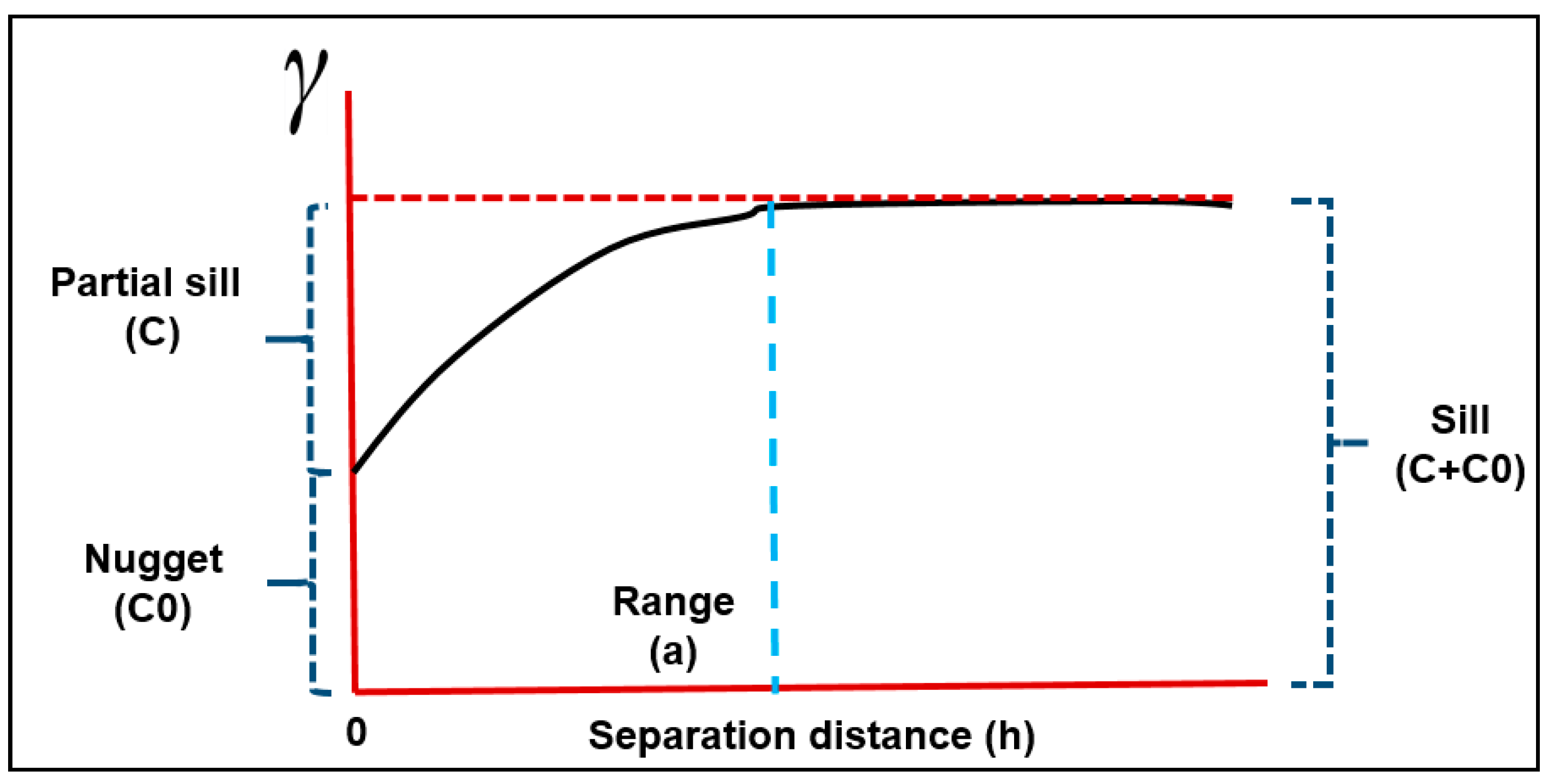
2.7. Semivariogram Analysis

A semivariogram is a statistical tool that evaluates how much two random variables’ average degree of similarity decreases as their distance from one another rises. According to [49], it shows the measured sample points’ spatial autocorrelation. The predicted values from the PLSR models were interpolated using ordinary kriging (OK). The value of the soil parameters at an unsampled location was ascertained using a set of analytical techniques using the OK geostatistics framework. The spatial continuity between points is characterized by the semivariance function. A semivariogram is created when the semivariance is plotted against the lag distance or separation distance between the dots.

Lark [50]. Nugget semivariance, range, and sill were found to be the model’s parameters (Figure 3). Range is defined as the distance beyond which observations are not spatially dependent [51]; sill is the lag distance between measurements at which one value for a variable does not influence neighboring values; and nugget semivariance is the variance at zero distance and represents the experimental error and field variation within the minimum sampling spacing, as seen in Abuzaid [52].

The spatial dependency (SPD) is defined by the hint(C0)/sill(C0 + C) ratio, where ratios less than 0.25, 0.25–0.75, and above 0.75 indicate a strong, moderate, and weak SPD, respectively [53,54]. To ensure the models’ validity and to compare the estimated values from the semivariogram model with the actual values, the models underwent cross-validation (a process including trial and error). The cross-validation statistics mean error (ME), mean standardized error (MSE), and root mean square standardized error (RMSSE) are used to quantify differences between estimated and experimental values [55]. The semivariogram models’ parameters were cross-validated and then utilized to create maps for CEC using ordinary kriging interpolation in ArcGIS 10.4. The kriging method was applied using the following Equation (7), which was provided by [56]. Based on the lowest ME and MSE (around zero), comparable values of RMSE and ASE, and RMSSE close to unity, the best-fit model was chosen [57,58].

$$Z^{\mathrm{*}}(Xo)=\sum _{(i=1)}^N\mathsf{\lambda }\mathrm{i}{Z}^{\mathrm{*}}\left(\mathrm{x}\mathrm{i}\right)$$

(7)

where $Z^{\mathrm{*}}\left(Xo\right)$ is the estimated variable at location xo, Z^*(Xi) is the value of an inspected variable at location Xi, N is the number of observations in the vicinity of the inspected point, and λi is the statistical weight assigned to Z^*(Xi) for a sample near $Xo$.

3. Results and Discussion

3.1. Descriptive Statistics of Soil Samples

Table 3. Summary of descriptive statistical analysis of the investigated soil parameters.

Properties	Mean	Minimum	Maximum	Standard Deviation
Sand (%)	40.27	25.05	74.34	9.14
Silt (%)	33.80	22.11	60.91	6.21
Clay (%)	25.93	13.56	49.05	8.07
CEC (cmolc kg−1)	22.72	17.91	30.35	2.66
EC (dSm−1)	4.01	0.80	11.00	2.75
pH	7.31	7.73	8.48	0.45

presents an overview of the descriptive statistical analysis of the soil parameters that were examined. The soils ranged in pH from a low of 7.73 to a maximum of 8.48. This shows that the study area’s conditions are slightly to highly alkaline [59]. The pH of the soil greatly affects the nutrients that are available to plants. Iron, zinc, and other micronutrients are less available to plants when the pH of the soil is too high [60]. As a result, sustaining an appropriate pH range in the soil is essential for plant growth and nutrient availability [60]. Furthermore, increased soil pH causes a rise in the mineralizable portions of N and C ratios, where the connections between organic elements and clays are broken [61]. According to the data, the soils in the research area have slight to high salinity, with average EC values of 4.01 ± 2.75 dSm⁻¹ and a range of 0.80 to 11 dSm⁻¹ [62]. The amounts of sand, silt, and clay in the soil range from 5.05 to 74.34%, 9.07 to 60.91% and 13.56 to 49.05%, respectively. There were differences in soil textures between loam, clay, clay loam, silty loam, silty clay loam, sandy loam, sandy clay loam, sandy clay, and silty clay (Figure 4). These soils’ cation exchange capacity is moderate, with a mean value of 22.72 cmolc kg⁻¹. The CEC in the studied area ranges widely, from 17.91 to 30.35 cmolc kg⁻¹ soil, with an average of 22.72 ± 2.66 cmolc kg⁻¹ soils. The high values of CEC and basic alkali cation adsorption are correlated with clay content [63]. The interpolation maps of EC and pH values are given in Figure 4a,b.

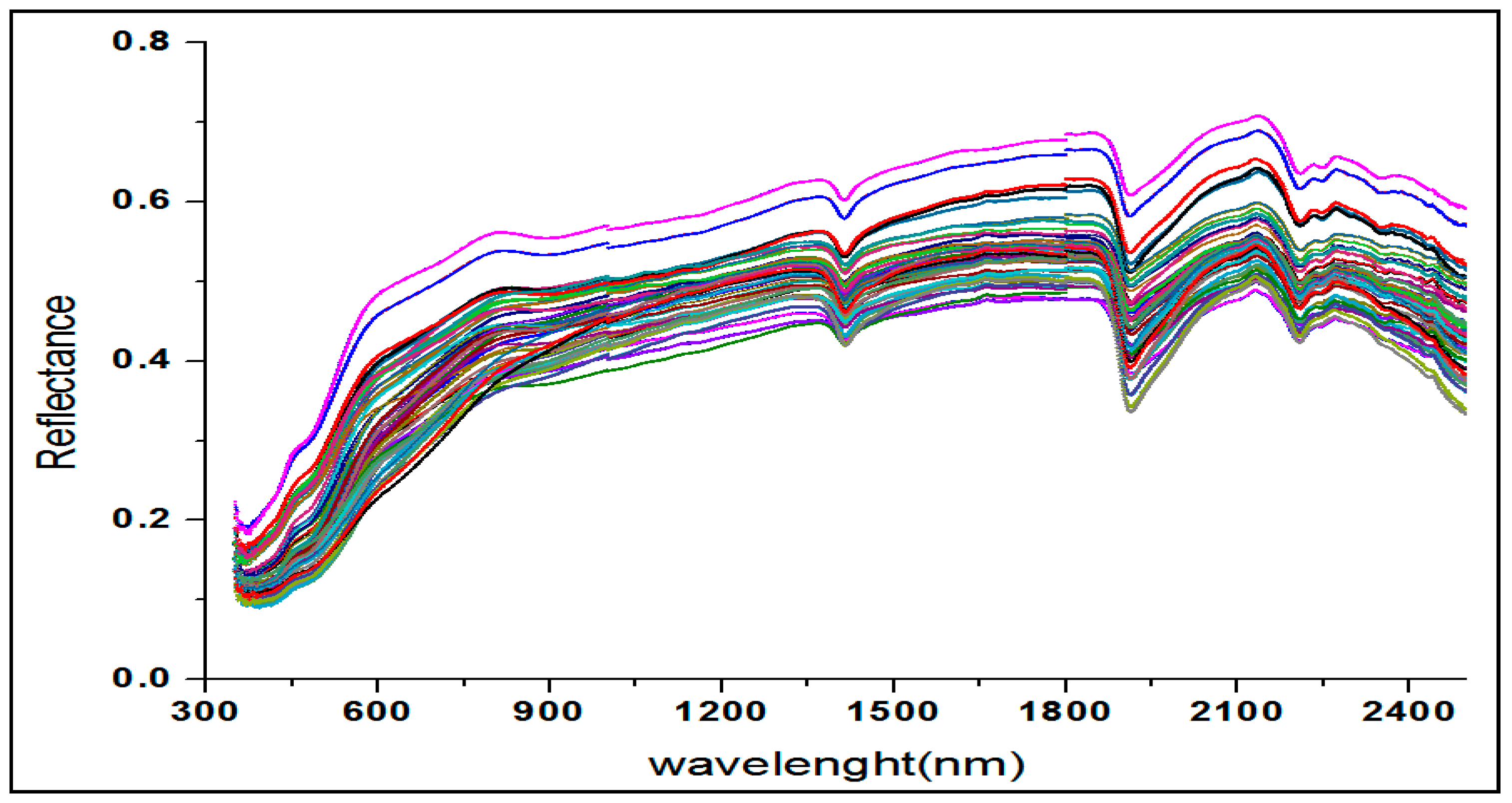
3.2. Qualitative Description of the Soil Spectra

Spectral reflectance characteristics (Figure 5) aid in the identification of the main parameters of the soil, including organic matter, clay content, moisture content, cation exchange capacity, soil color, effect of soil minerals, soil surface condition, salinity, and alkalinity. The spectra library was created using reflectance spectra produced by laboratory experiments, and reflectance transformations were applied to further analyses of the spectra. In the Vis-NIR range, all of the soil samples showed distinctive reflectance spectra that corresponded to different molecular groups or chemical and/or mineralogical components [64]. There were noticeable absorption peaks and regions at wavelengths of 1400, 1900, and 2200 nm. Lower reflectance values were seen in the visible region (400–700 nm), which increased gradually in the near-infrared region (700–2500 nm). The hydroxyl group of free water is linked to the peaks at 1400 and 1900 nm, while clay minerals and lattice–OH features are linked to the absorption features at 1400 and 2200 nm [14,44]. Furthermore, the 2200 nm characteristic is linked to different organic functional groups in different clay minerals, such as CH₂, CH₃, etc., SiOH bonds, or cation–hydroxyl bonds [65] (for various layers, the OH stretching absorption feature was measured between 1410 and 1415 nm, the H–O–H absorption feature between 1910 and 1920 nm, and the Al–OH stretching between 2200 and 2210 nm). Furthermore, the absorption characteristics linked to the soil organic matter components were detected between 2390 and 2400 nm [66].

The average spectral library of CEC values is used for the different reflectance conversions. Figure 6 provides examples of various modifications. In addition to their impacts on strengthening the various absorption properties, the various transformations also served to lessen the various kinds of sounds in spectra.

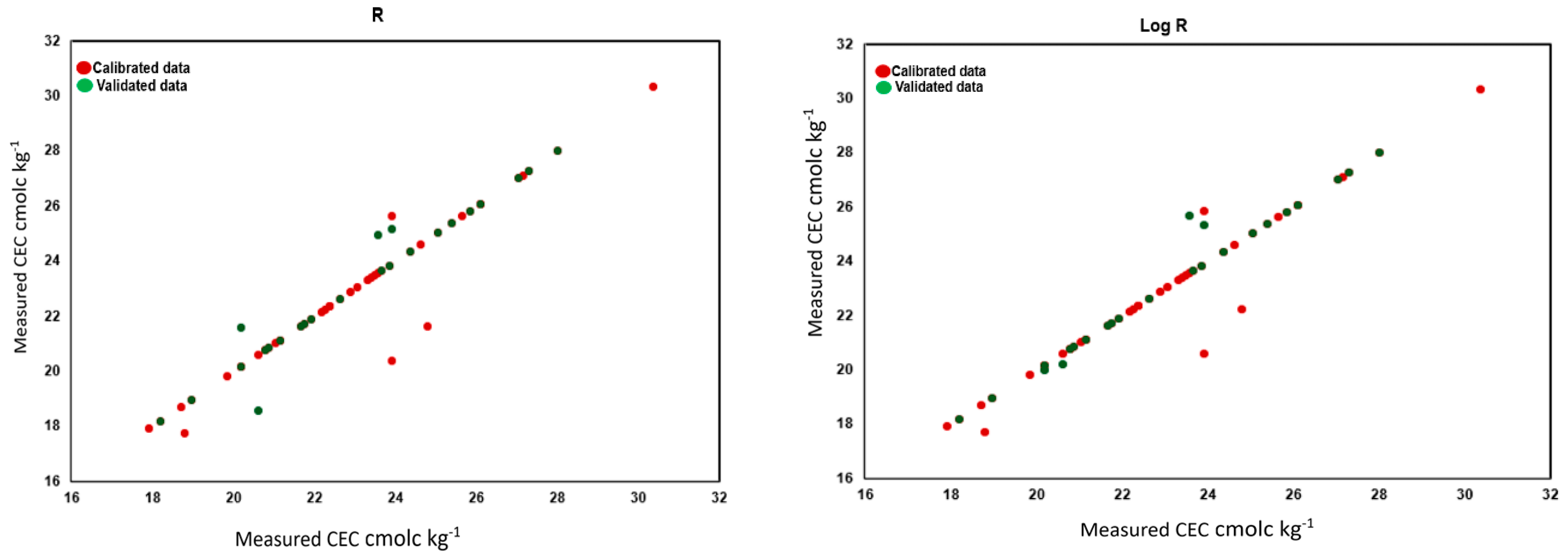
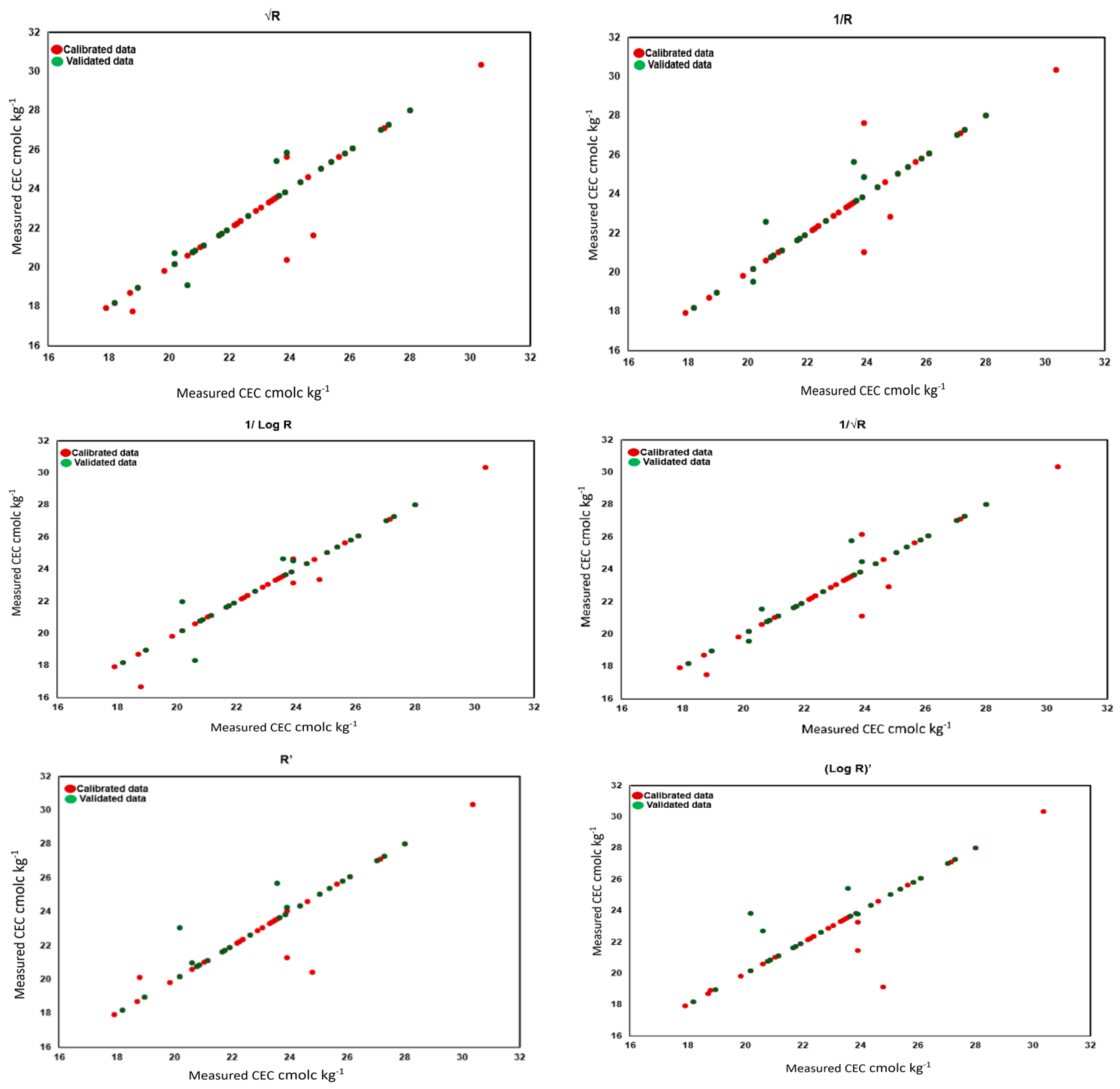
3.3. Prediction of Soil Properties Using PLSR

The most widely used multivariate quantifiable technique in soil research for chemometrics is PLSR, according to [67]. In order to assess soil attributes, this strategy adjusts soil reflectance [44]. It is superior to traditional methods for handling multi-collinearity in high-dimensional data. From each partial least square analysis, the following values were obtained: regression coefficients (R²), residual prediction deviation (RPD), root mean square error (RMSE), and the ratio of performance to inter-quartile range (RPIQ). The coefficient of determination, residual predictive deviation, root mean square error, and performance-to-IQ ratio are commonly used assessment metrics for Vis-NIR model analysis [68,69,70]. R² and RMSE are useful metrics for assessing the models’ accuracy. Since these models exhibit similar stability at the same RPD level, RPD and RPIQ can be used to analyze the stability [46].

The PLSR model was also used to estimate the cross-validation segments, correlation loadings factor, and scatter plots of the measured vs. predicted soil parameters (

Table 4. CEC prediction models’ performance with the matching preprocessing transformation.

No.	Spectral Transformation	Calibrated (N = 73)				Validated (N = 31)
		R2	RMSE	RPD	RPIQ	R2	RMSE	RPD	RPIQ
1	1/Log R	0.98	0.40	6.99	9.22	0.89	0.85	3.28	4.31
2	R	0.95	0.60	4.69	6.53	0.90	0.83	3.40	4.94
3	1/√R	0.95	0.62	4.55	6.29	0.93	0.68	4.02	6.50
4	(1/Log R)’	0.94	0.65	4.23	6.07	0.88	0.89	2.90	4.88
5	Log R	0.94	0.69	4.09	5.83	0.93	0.69	4.04	6.50
6	√R	0.93	0.76	3.79	5.39	0.89	0.86	3.34	5.52
7	R’	0.92	0.77	3.57	4.81	0.86	0.96	2.66	4.52
8	1/R	0.90	0.85	3.47	4.61	0.90	0.83	3.30	5.31
9	(√R)’	0.91	0.82	3.36	4.50	0.83	1.06	2.43	4.89
10	(Log R)’	0.89	0.90	3.09	4.08	0.77	1.23	2.01	2.99
11	(1/√R)’	0.82	1.16	2.40	3.19	0.51	1.21	0.99	1.17
12	(1/R)’	0.75	1.37	2.06	2.71	0.50	1.33	1.13	1.33
13	(1/Log R)”	0.75	1.37	2.05	2.68	0.42	1.35	1.09	1.28
14	R”	0.58	1.78	1.66	2.06	0.35	1.81	0.88	1.04
15	(√R)”	0.53	1.88	1.60	1.96	0.37	2.10	1.00	1.18
16	(Log R)”	0.52	1.90	1.62	1.95	0.41	1.88	1.28	1.50
17	(1/√R)”	0.28	2.27	1.48	1.68	0.21	2.31	1.21	1.43
18	(1/R)”	0.42	5.25	0.74	0.73	0.33	4.86	0.99	1.16

and Figure 7). Although they are less common [17], predictions of secondary attributes using Vis-NIR data have also been reported in a number of other temperate soil studies, including those by Abdul Munnaf [16] for pH, ex-Na, ex-Ca, ex-Mg, and ex-K (0.58 ≤ R² ≥ 0.81), Mouazen and Kuang [71] for ex P (R² = 0.60), and Ulusoy et al. [2] for CEC (0.70 ≤ R² ≥ 0.75).

Table 4 provides a statistical summary of the PLSR models created for CEC prediction using different spectral modifications. Only those modifications that, after calibration and cross-validation, produced models with a moderate-to-high coefficient of determination (R² > 0.6) are included here. These were chosen based on the cross-validation procedure’s outcomes; namely, the lowest RMSE values and highest R², RPD, and RPIQ values. Out of the 18 reflectance transformations that were combined with reflectance spectra, 13 produced results that were adequate for both the model calibration and validation stages (Table 4). Conversely, the models that were produced by the second derivative spectrum of R, Log R, √R, reciprocal of R, and root R were not well calibrated. Based on the values of R², RMSE, RPD, and RPIQ in the calibration and validation datasets, the best fits of the 13 reflectance transformations were chosen. Ten transformation techniques produced calibration models for the current study that were satisfactory (Table 4), with R² > 0.6, RPD > 2.5, and RPIQP > 4.05. The reciprocal of Log R transformation (R² = 0.98, RMSE = 0.40, RPD = 6.99, and RPIQ = 9.22) was the most effective transformation and calibration model for assessing CEC in Vis-NIR spectra. This suggests that the best model for predicting CEC values is produced by combining the reciprocal of Log R with PLSR.

The RPD values of three transformations, namely, (1/R)’, (1/√R)’, and (1/Log R)”, ranged between 2 and 2.5, indicating that employing these transformations resulted in excellent modeling of CEC using PLSR analysis. In contrast, the performance of the second derivative of R, Log R, root R, and reciprocal of root R was mediocre. The modeling is really bad because only the second derivative of the (1/R) transformation has an RPD smaller than one.

3.4. CEC Mapping Based on Semivariogram Analysis

The degree to which the results are acceptable and compatible with previous studies is demonstrated by the accuracy of the spatial distribution map of CEC created using OK [72]. The semivariogram function in the context of the geostatistical analysis examines the null hypothesis, according to which the soil variable does not show spatial dependency at the selected lag h. The spatial dependence for CEC in the research area (

Table 5. Geostatistical parameters for CEC in the soil of the study area.

Spatial Distribution Model	R2	RMSE	MSE	RMSSE	Range (m)	Nugget	Partial Sill	Sill	Nugget/Sill Ratios	Spatial Dependence
Spherical	0.96	2.55	−0.003	1.018	14,846.4	4.78	2.35	7.13	0.67	Moderate
Exponential	0.95	2.56	−0.005	1.025	13,878.2	3.68	3.53	7.21	0.51	Moderate
Gaussian	0.88	2.55	−0.004	1.018	12,886.0	2.21	1.93	4.14	0.53	Moderate
Circular	0.94	2.55	−0.004	1.017	13,785.0	4.91	2.24	7.14	0.68	Moderate

) and the small nugget semivariance indicate that the lag h appears to characterize the spatial variation, and the lag h scale well matched the spatial variation of CEC. Therefore, it is not necessary to sample this variable again in order to identify spatial dependence.

In situations when there is a high or moderate spatial correlation between the distributions of soil attributes, the range of the semivariogram indicates the average extent of these patches. Table 5 indicates that for the models—spherical, exponential, Gaussian, and circular models—the RMSSE values were 1.018, 1.025, 1.018, and 1.019, and the MSE values were −0.003, −0.005, −0.004, and −0.004, accordingly. For all parameters, the RMSSE values were near one and the MSE values were near zero [73]. This suggests that OK was a suitable and trustworthy method for estimating the CEC’s spatial distribution in the research area [72].

At the large scale, CEC values displayed a moderate geographic correlation, indicating that both extrinsic and intrinsic influences were present. Because of their strong spatial dependence, it was therefore reasonable to forecast the spatial distribution of CEC at a wide scale. Furthermore, there were minor variations within the ranges of different models of spatial distribution. Extrinsic (soil management techniques, such as fertilization) and intrinsic (soil formation factors, like soil parent materials) factors can both have an impact on the spatial variability of soil parameters. According to [53,54], intrinsic factors are typically responsible for soil qualities that exhibit great geographical dependency, while extrinsic factors are responsible for those that exhibit weak spatial dependency. A larger range indicates that observed values of the CEC variable are influenced by other values of this variable over greater distances than soil variables, which have smaller ranges [74]. This shows that, at longer distances, CEC levels had an impact on nearby sand values. In the study region, Figure 8 shows the regional distribution of the CEC.

4. Conclusions

Comprehending the principles of cation exchange facilitates well-informed decision-making about soil management, fertilization with nutrients, preservation of the total fertility of agricultural and natural ecosystems, and attaining agricultural sustainability. Vis-NIR spectroscopy is an extremely useful method for CEC evaluation. The modeling of the correlation between the spectral response and the CEC concentrations served as the foundation for the current investigation. To be more specific, the PLSR was used to map and forecast CEC in situ analysis and Vis-NIR spectroscopy using the reflectance spectra obtained in the dry conditions of thirty-one soil samples were chosen in order to confirm the accuracy of the findings. The spatial variety and features of the samples that were chosen at random comprised the study region. Ten transformation approaches produced calibration models, with R² > 0.6, RPD > 2.5, and RPIQ > 4.05. These results show that the methods met the study’s requirements. The reciprocal of Log R transformation (R² = 0.98, RMSE = 0.40, RPD = 6.99, and RPIQ = 9.22) was the most effective transformation and calibration model for assessing CEC in Vis-NIR spectra. This suggests that PLSR and the reciprocal of Log R can be combined to provide the best model for predicting CEC values. Four models—Gaussian, exponential, circular, and spherical—fit the CEC values the best. The techniques used here allow for the rapid and widespread use of a “quick”, inexpensive tool. We put forth the overall proposal that the efficient monitoring of soil conditions through the use of earth observation instruments can be further enhanced in the future on a multi-scale and multi-parameter scale by combining information derived from earth observation with socioeconomic factors such as population, economy, etc. This will provide an integrated system that can be operationally adjusted to support and enhance local government efficiency. Additional investigation is required to examine various datasets obtained from an increased number of fields with varying soil types, textural attributes, land uses, and climate conditions.

References

1. Demattê, J.A.; Ramirez-Lopez, L.; Marques, K.; Rodella, A. Chemometric soil analysis on the determination of specific bands for the detection of magnesium and potassium by spectroscopy. Geoderma 2017, 288, 8–22. [Google Scholar] [CrossRef]
2. Ulusoy, Y.; Tekin, Y.; Tümsavaş, Z.; Mouazen, A.M. Prediction of soil cation exchange capacity using visible and near infrared spectroscopy. Biosyst. Eng. 2016, 152, 79–93. [Google Scholar] [CrossRef]
3. Fung, E.; Wang, J.; Zhao, X.; Farzamian, M.; Allred, B.; Clevenger, W.B.; Levison, P.; Triantafilis, J.J.S.; Research, T. Mapping cation exchange capacity and exchangeable potassium using proximal soil sensing data at the multiple-field scale. Soil Tillage Res. 2023, 232, 105735. [Google Scholar] [CrossRef]
4. Emamgolizadeh, S.; Bateni, S.; Shahsavani, D.; Ashrafi, T.; Ghorbani, H. Estimation of soil cation exchange capacity using Genetic Expression Programming (GEP) and Multivariate Adaptive Regression Splines (MARS). J. Hydrol. 2015, 529, 1590–1600. [Google Scholar] [CrossRef]
5. Rhoades, J.D. Cation exchange capacity. In Methods of Soil Analysis: Part 2 Chemical and Microbiological Properties, 9.2.2, 2nd ed.; Wiley Online Library: Hoboken, NJ, USA, 1982; Volume 9, pp. 149–157. [Google Scholar]
6. Richards, L.A. Diagnosis and Improvement of Saline and Alkali Soils; US Government Printing Office: Washington, DC, USA, 1954. [Google Scholar]
7. Polemio, M.; Rhoades, J.D. Determining Cation Exchange Capacity: A New Procedure for Calcareous and Gypsiferous Soils. Soil Sci. Soc. Am. J. 1977, 41, 524–528. [Google Scholar] [CrossRef]
8. Takele, C.; Iticha, B. Use of infrared spectroscopy and geospatial techniques for measurement and spatial prediction of soil properties. Heliyon 2020, 6, e05269. [Google Scholar] [CrossRef] [PubMed]
9. Keshavarzi, A.; Sarmadian, F.; Shiri, J.; Iqbal, M.; Tirado-Corbalá, R.; Omran, E.-S.E. Application of ANFIS-based subtractive clustering algorithm in soil Cation Exchange Capacity estimation using soil and remotely sensed data. Measurement 2017, 95, 173–180. [Google Scholar] [CrossRef]
10. Mishra, G.; Sulieman, M.M.; Kaya, F.; Francaviglia, R.; Keshavarzi, A.; Bakhshandeh, E.; Loum, M.; Jangir, A.; Ahmed, I.; Elmobarak, A.; et al. Machine learning for cation exchange capacity prediction in different land uses. CATENA 2022, 216, 106404. [Google Scholar] [CrossRef]
11. Kania, M.; Gruba, P. Estimation of selected properties of forest soils using near-infrared spectroscopy (NIR). Soil Sci. Annu. 2016, 67, 32–36. [Google Scholar] [CrossRef]
12. Rehman, H.U.; Knadel, M.; de Jonge, L.W.; Moldrup, P.; Greve, M.H.; Arthur, E. Comparison of Cation Exchange Capacity Estimated from Vis–NIR Spectral Reflectance Data and a Pedotransfer Function. Vadose Zone J. 2019, 18, 1–8. [Google Scholar] [CrossRef]
13. Waruru, B.K.; Shepherd, K.D.; Ndegwa, G.M.; Kamoni, P.T.; Sila, A.M. Rapid estimation of soil engineering properties using diffuse reflectance near infrared spectroscopy. Biosyst. Eng. 2014, 121, 177–185. [Google Scholar] [CrossRef]
14. Ben-Dor, E. Quantitative remote sensing of soil properties. Adv. Agron. 2002, 75, 173–243. [Google Scholar]
15. Demattê, J.A.M. Characterization and discrimination of soils by their reflected electromagnetic energy. Pesqui. Agropecuária Bras. 2002, 37, 1445–1458. [Google Scholar] [CrossRef]
16. Abdul Munnaf, M.; Nawar, S.; Mouazen, A.M. Estimation of Secondary Soil Properties by Fusion of Laboratory and On-Line Measured Vis–NIR Spectra. Remote Sens. 2019, 11, 2819. [Google Scholar] [CrossRef]
17. Stenberg, B.; Viscarra-Rossel, R.A.; Mouazen, A.M.; Wetterlind, J. Visible and Near Infrared Spectroscopy in Soil Science. Adv. Agron. 2010, 107, 163–215. [Google Scholar] [CrossRef]
18. Nocita, M.; Stevens, A.; Noon, C.; van Wesemael, B. Prediction of soil organic carbon for different levels of soil moisture using Vis-NIR spectroscopy. Geoderma 2013, 199, 37–42. [Google Scholar] [CrossRef]
19. Xu, S.; Zhao, Y.; Wang, M.; Shi, X. Comparison of multivariate methods for estimating selected soil properties from intact soil cores of paddy fields by Vis–NIR spectroscopy. Geoderma 2018, 310, 29–43. [Google Scholar] [CrossRef]
20. Fan, S.; Wang, X.; Lei, J.; Ran, Q.; Ren, Y.; Zhou, J. Spatial distribution and source identification of heavy metals in a typical Pb/Zn smelter in an arid area of northwest China. Hum. Ecol. Risk Assess. Int. J. 2019, 25, 1661–1687. [Google Scholar] [CrossRef]
21. Mondal, B.P.; Sekhon, B.S.; Sahoo, R.N.; Paul, P. Vis-nir reflectance spectroscopy for assessment of soil organic carbon in a rice-wheat field of ludhiana district of punjab. ISPRS-Int. Arch. Photogramm. Remote Sens. Spat. Inf. Sci. W6. [CrossRef]
22. Conforti, M.; Castrignanò, A.; Robustelli, G.; Scarciglia, F.; Stelluti, M.; Buttafuoco, G. Laboratory-based Vis–NIR spectroscopy and partial least square regression with spatially correlated errors for predicting spatial variation of soil organic matter content. CATENA 2015, 124, 60–67. [Google Scholar] [CrossRef]
23. Curcio, D.; Ciraolo, G.; D’asaro, F.; Minacapilli, M. Prediction of Soil Texture Distributions Using VNIR-SWIR Reflectance Spectroscopy. Procedia Environ. Sci. 2013, 19, 494–503. [Google Scholar] [CrossRef]
24. Mousavi, F.; Abdi, E.; Ghalandarzadeh, A.; Bahrami, H.A.; Majnounian, B.; Ziadi, N. Diffuse reflectance spectroscopy for rapid estimation of soil Atterberg limits. Geoderma 2019, 361, 114083. [Google Scholar] [CrossRef]
25. Yitagesu, F.A.; Van der Meer, F.; Van der Werff, H.; Hecker, C. Spectral characteristics of clay minerals in the 2.5–14 μm wavelength region. Appl. Clay Sci. 2011, 53, 581–591. [Google Scholar] [CrossRef]
26. Vasques, G.M.; Grunwald, S.; Sickman, J.O. Modeling of soil organic carbon fractions using visible–near-infrared spectroscopy. Appl. Clay Sci. 2009, 73, 176–184. [Google Scholar] [CrossRef]
27. Kaya, F.; Mishra, G.; Francaviglia, R.; Keshavarzi, A. Combining Digital Covariates and Machine Learning Models to Predict the Spatial Variation of Soil Cation Exchange Capacity. Land 2023, 12, 819. [Google Scholar] [CrossRef]
28. Saidi, S.; Ayoubi, S.; Shirvani, M.; Azizi, K.; Zeraatpisheh, M. Comparison of Different Machine Learning Methods for Predicting Cation Exchange Capacity Using Environmental and Remote Sensing Data. Sensors 2022, 22, 6890. [Google Scholar] [CrossRef]
29. Mishra, G.; Das, J.; Sulieman, M. Modelling Soil Cation Exchange Capacity in Different Land-Use Systems using Artificial Neural Networks and Multiple Regression Analysis. Curr. Sci. 2019, 116, 2020–2027. [Google Scholar] [CrossRef]
30. Fang, Q.; Hong, H.; Zhao, L.; Kukolich, S.; Yin, K.; Wang, C. Visible and Near-Infrared Reflectance Spectroscopy for Investigating Soil Mineralogy: A Review. J. Spectrosc. 2018, 2018, 3168974. [Google Scholar] [CrossRef]
31. Soriano-Disla, J.M.; Janik, L.J.; Rossel, R.A.V.; Macdonald, L.M.; McLaughlin, M.J. The Performance of Visible, Near-, and Mid-Infrared Reflectance Spectroscopy for Prediction of Soil Physical, Chemical, and Biological Properties. Appl. Spectrosc. Rev. 2013, 49, 139–186. [Google Scholar] [CrossRef]
32. Mustafa, A.A.; Engineering, A. Incorporate the Fertility Capability Classification and Geo-informatics for Assessing Soil: A Case Study on Some Soils of Sohag Governorate, Egypt. J. Soil Sci. Agric. Eng. 2023, 14, 187–193. [Google Scholar] [CrossRef]
33. El-Rawy, M.; Abdalla, F.; El Alfy, M.; El-Rawy, M.; Abdalla, F.; El Alfy, M.; Abdalla, F. Water resources in Egypt. In The Geology of Egypt; Springer: Berlin/Heidelberg, Germany, 2019; pp. 687–711. [Google Scholar]
34. Rhoades, J.D. Salinity: Electrical conductivity and total dissolved solids. In Methods of Soil Analysis: Part 3; SSSA Book Series No. 5, SSSA and ASA; SSSA Inc.: Madison, WI, USA; ASA Inc.: Madison, WI, USA, 1996; pp. 417–435. [Google Scholar]
35. Thomas, G.W. Soil pH and Soil Acidity. In Method of Soil Analysis, Part 3: Chemical Methods; SSSA Inc.: Madison, WI, USA; ASA Inc.: Madison, WI, USA, 1996; pp. 475–490. [Google Scholar]
36. Sumner, M.E.; Miller, W.P. Cation exchange capacity and exchange coefficients. In Methods of Soil Analysis. Part 3. Chemical Methods; Bingham, J.M., Ed.; ASA-SSSA: Madison, WI, USA, 1996; Volume 5, pp. 1201–1229. [Google Scholar]
37. Lavkulich, L.M. Methods Manual: Pedology Laboratory; University of British Columbia, Department of Soil Science: Vancouver, BC, Canada, 1981. [Google Scholar]
38. Asgari, N.; Ayoubi, S.; Demattê, J.A.M.; Dotto, A.C. Carbonates and organic matter in soils characterized by reflected energy from 350–25000 nm wavelength. J. Mt. Sci. 2020, 17, 1636–1651. [Google Scholar] [CrossRef]
39. Savitzky, A.; Golay, M.J.E. Smoothing and Differentiation of Data by Simplified Least Squares Procedures. Anal. Chem. 1964, 36, 1627–1639. [Google Scholar] [CrossRef]
40. Gholizadeh, A.; Borůvka, L.; Saberioon, M.; Vašát, R. Visible, Near-Infrared, and Mid-Infrared Spectroscopy Applications for Soil Assessment with Emphasis on Soil Organic Matter Content and Quality: State-of-the-Art and Key Issues. Appl. Spectrosc. 2013, 67, 1349–1362. [Google Scholar] [CrossRef]
41. Jinliang, W.; Qiming, Q.; Heng, D.; Chao, C.; Qingye, M. Study on quantitative retrieval of soil organic matter based on bare soil spectrum. In Proceedings of the 3rd International Conference on Multimedia Technology (ICMT-13); Atlantis Press: Amsterdam, The Netherlands, 2013; pp. 382–389. [Google Scholar]
42. Li, J.; Deng, X.; Wang, Y.; Fu, Y.; Li, E.; Peng, M. Quantitative prediction of soil organic matter of mined-land by hyperspectral remote sensing and mathematical statistics. Sens. Transducers 2014, 162, 227. [Google Scholar]
43. Næs, T.; Isaksson, T.; Fearn, T.; Davies, T. A User-Friendly Guide to Multivariate Calibration and Classification, 2nd ed.; NIR Publiscations: Chichester, UK, 2017. [Google Scholar] [CrossRef]
44. Viscarra Rossel, R.A.; Walvoort, D.J.J.; McBratney, A.B.; Janik, L.J.; Skjemstad, J.O. Visible, near infrared, mid infrared or combined diffuse reflectance spectroscopy for simultaneous assessment of various soil properties. Geoderma 2006, 131, 59–75. [Google Scholar] [CrossRef]
45. Aslam, M.W.; Wajid, M.; Waheed, A.; Ahmad, S.; Jafar, K.; Akmal, H.; Khan, T.; Maqsud, M.S.; Khan, M.S. Revision of some mensural measurements, food preference, and haematological parameters in breeding pairs of blue rock pigeon, Columba livia sampled from punjab Pakistan. Braz. J. Biol. 2023, 83, e252059. [Google Scholar] [CrossRef]
46. Maurel, V.B.; Fernandez-Ahumada, E.; Palagos, B.; Roger, J.; McBratney, A. Prediction of soil attributes by NIR spectroscopy. A critical review of chemometric indicators commonly used for assessing the quality of the prediction. Trends Anal. Chem. 2010, 29, 1073–1081. [Google Scholar] [CrossRef]
47. Jin, X.; Li, S.; Zhang, W.; Zhu, J.; Sun, J. Prediction of Soil-Available Potassium Content with Visible Near-Infrared Ray Spectroscopy of Different Pretreatment Transformations by the Boosting Algorithms. Appl. Sci. 2020, 10, 1520. [Google Scholar] [CrossRef]
48. Terra, F.S.; Demattê, J.A.M.; Viscarra Rossel, R.A. Spectral libraries for quantitative analyses of tropical Brazilian soils: Comparing vis–NIR and mid-IR reflectance data. Geoderma 2015, 255–256, 81–93. [Google Scholar] [CrossRef]
49. Singha, C.; Swain, K.C.; Sahoo, S.; Govind, A. Prediction of soil nutrients through PLSR and SVMR models by VIs-NIR reflectance spectroscopy. Egypt. J. Remote Sens. Space Sci. 2023, 26, 901–918. [Google Scholar] [CrossRef]
50. Lark, R.M. A comparison of some robust estimators of the variogram for use in soil survey. Eur. J. Soil Sci. 2000, 51, 137–157. [Google Scholar] [CrossRef]
51. Goenster-Jordan, S.; Jannoura, R.; Jordan, G.; Buerkert, A.; Joergensen, R.G. Spatial variability of soil properties in the floodplain of a river oasis in the Mongolian Altay Mountains. Geoderma 2018, 330, 99–106. [Google Scholar] [CrossRef]
52. Abuzaid, A.S.; Jahin, H.S.; Shokr, M.S.; El Baroudy, A.A.; Mohamed, E.S.; Rebouh, N.Y.; Bassouny, M.A. A Novel Regional-Scale Assessment of Soil Metal Pollution in Arid Agroecosystems. Agronomy 2023, 13, 161. [Google Scholar] [CrossRef]
53. Cambardella, C.A.; Moorman, T.B.; Novak, J.M.; Parkin, T.B.; Karlen, D.L.; Turco, R.F.; Konopka, A.E. Field-Scale Variability of Soil Properties in Central Iowa Soils. Soil Sci. Soc. Am. J. 1994, 58, 1501–1511. [Google Scholar] [CrossRef]
54. Dad, J.M.; Shafiq, M.U. Spatial variability and delineation of management zones based on soil micronutrient status in apple orchard soils of Kashmir valley, India. Environ. Monit. Assess. 2021, 193, 797. [Google Scholar] [CrossRef]
55. Isaaks, E.H.; Srivastava, R.M. Applied Geostatistics; Oxford University Press: New York, NY, USA, 1989. [Google Scholar]
56. Cafarelli, B.; Castrignanò, A.; De Benedetto, D.; Palumbo, A.D.; Buttafuoco, G. A linear mixed effect (LME) model for soil water content estimation based on geophysical sensing: A comparison of an LME model and kriging with external drift. Environ. Earth Sci. 2014, 73, 1951–1960. [Google Scholar] [CrossRef]
57. Sebei, A.; Chaabani, A.; Abdelmalek-Babbou, C.; Helali, M.A.; Dhahri, F.; Chaabani, F. Evaluation of pollution by heavy metals of an abandoned Pb-Zn mine in northern Tunisia using sequential fractionation and geostatistical mapping. Environ. Sci. Pollut. Res. 2020, 27, 43942–43957. [Google Scholar] [CrossRef] [PubMed]
58. Mallik, S.; Mishra, U.; Paul, N. Groundwater suitability analysis for drinking using GIS based fuzzy logic. Ecol. Indic. 2020, 121, 107179. [Google Scholar] [CrossRef]
59. Baruah, T.; Borthakur, H.P. Soil Chemistry. In A Textbook of Soil Analysis; Vikas Publishing House Pvt. Ltd.: New Delhi, India, 1997; pp. 118–132. [Google Scholar]
60. Dewangan, S.; Kumari, L.; Minj, P.; Kumari, J.; Sahu, R. The effects of soil ph on soil health and environmental sustainability: A review. JETIR 2023, 10, 611–616. [Google Scholar]
61. Curtin, D.; Campbell, C.; Jalil, A. Effects of acidity on mineralization: pH-dependence of organic matter mineralization in weakly acidic soils. Soil Biol. Biochem. 1998, 30, 57–64. [Google Scholar] [CrossRef]
62. Food and Agriculture Organization of the United Nations. A Provisional Methodology for Soil Degradation Assessment; FAO: Rome, Italy, 1980. [Google Scholar]
63. Abdel-Fattah, M.K.; Mohamed, E.S.; Wagdi, E.M.; Shahin, S.A.; Aldosari, A.A.; Lasaponara, R.; Alnaimy, M.A. Quantitative Evaluation of Soil Quality Using Principal Component Analysis: The Case Study of El-Fayoum Depression Egypt. Sustainability 2021, 13, 1824. [Google Scholar] [CrossRef]
64. Demattê, J.A.M.; da Silva Terra, F. Spectral pedology: A new perspective on evaluation of soils along pedogenetic alterations. Geoderma 2014, 217–218, 190–200. [Google Scholar] [CrossRef]
65. Poppiel, R.R.; Lacerda, M.P.C.; Oliveira, M.P.D.; Demattê, J.A.M.; Romero, D.J.; Sato, M.V.; Almeida, L.R.D.; Cassol, L.F.M. Surface Spectroscopy of Oxisols, Entisols and Inceptisol and Relationships with Selected Soil Properties. Rev. Bras. Cienc. Solo 2018, 42, e0160519. [Google Scholar] [CrossRef]
66. Rizzo, R.; Demattê, J.A.M.; Terra, F.d.S. Using numerical classification of profiles based on Vis-NIR spectra to distinguish soils from the Piracicaba Region, Brazil. Rev. Bras. Cienc. Solo 2014, 38, 372–385. [Google Scholar] [CrossRef]
67. Adeline, K.; Gomez, C.; Gorretta, N.; Roger, J.-M. Predictive ability of soil properties to spectral degradation from laboratory Vis-NIR spectroscopy data. Geoderma 2016, 288, 143–153. [Google Scholar] [CrossRef]
68. Shao, Y.; He, Y. Nitrogen, phosphorus, and potassium prediction in soils, using infrared spectroscopy. Soil Res. 2011, 49, 166–172. [Google Scholar] [CrossRef]
69. Wang, W.-J.; Li, Z.; Wang, C.; Zheng, D.; Du, H. Prediction of Available Potassium Content in Cinnamon Soil Using Hyperspectral Imaging Technology. Spectrosc. Spectr. Anal. 2019, 39, 1579–1585. [Google Scholar]
70. Vasques, G.; Grunwald, S.; Sickman, J. Comparison of multivariate methods for inferential modeling of soil carbon using visible/near-infrared spectra. Geoderma 2008, 146, 14–25. [Google Scholar] [CrossRef]
71. Mouazen, A.M.; Kuang, B. On-line visible and near infrared spectroscopy for in-field phosphorous management. Soil Tillage Res. 2016, 155, 471–477. [Google Scholar] [CrossRef]
72. Mohamed, E.S.; Baroudy, A.A.E.; El-Beshbeshy, T.; Emam, M.; Belal, A.A.; Elfadaly, A.; Aldosari, A.A.; Ali, A.M.; Lasaponara, R. Vis-NIR Spectroscopy and Satellite Landsat-8 OLI Data to Map Soil Nutrients in Arid Conditions: A Case Study of the Northwest Coast of Egypt. Remote Sens. 2020, 12, 3716. [Google Scholar] [CrossRef]
73. Aldabaa, A.; Yousif, I.A.H. Geostatistical approach for land suitability assessment of some desert soils. Egypt. J. Soil Sci. 2020, 60, 195–209. [Google Scholar] [CrossRef]
74. Calvete, F.J.S.; Ramírez, J.C. Geoestadística: Aplicaciones a la Hidrogeología Subterránea; Centro Internacional de Métodos Numéricos en Ingeniería: Barcelona, Spain, 1996. [Google Scholar]
Figure 1. Location map of the studied area.
Sustainability 16 07002 g001
Figure 2. Soil sample locations over the study area.
Sustainability 16 07002 g002
Figure 3. The relationship between variogram parameters (nugget, partial sill, sill) and sample separation distance.
Sustainability 16 07002 g003
Figure 4. Interpolation maps of (a); pH and (b); EC dS m−1.; and (c) map of soil texture.
Sustainability 16 07002 g004
Figure 5. Reflectance spectra of the examined soil samples.
Sustainability 16 07002 g005
Figure 6. Examples of various reflectance transformations used in the study.
Sustainability 16 07002 g006aSustainability 16 07002 g006b
Figure 7. The best-performing models for CEC based on different transformation methods.
Sustainability 16 07002 g007aSustainability 16 07002 g007b
Figure 8. The spatial distribution of the CEC throughout the study region.
Sustainability 16 07002 g008