Abstract
Predicting and assessing urban traffic noise is crucial for environmental management. This paper establishes a traffic noise simulation method based on microscopic traffic simulation, utilizing a traffic simulation under a mixed distribution probability combining normal and exponential distributions. This method integrates a single-vehicle noise prediction model to compute the spatial distribution of noise. Comparison with empirical data demonstrates that the proposed model effectively predicts the level of traffic noise. The accuracy of the model is validated through comparison with measured data, showing minimum and maximum errors of 3.60 dB(A) and 4.37 dB(A), respectively. Additionally, the noise spatial results under microscopic traffic models are compared with those under line source models, revealing that the proposed model provides a more detailed and realistic noise spatial distribution. Furthermore, the noise variation patterns between stable and time-varying traffic flows are investigated. Results indicate that noise levels fluctuate under stable traffic flow, whereas under time-varying traffic flow, noise values exhibit a stepped change.
1. Introduction
As urbanization continues to advance, noise pollution in urban areas remains a significant issue. The compliance rate of traffic noise at night is merely as high as 74.4% [1], which means that mitigating noise exposure is essential to prevent complaints [2]. The WHO [3] categorizes traffic noise as a significant health factor. Studies [4,5,6,7] further indicate that traffic noise has adverse effects on human health apart from work efficiency [8], potentially causing premature mortality and various psychological or physiological disorders, such as sleep disorders [9], annoyance [10], learning impairment [11], heart disease [12,13], and diastolic blood pressure [14]. Beyond acoustic energy exposure, factors related to sound signals significantly affect perception, such as peak levels, temporal variations, amplitude modulation, impulsivity, and frequency distribution [15,16,17].
In the numerous sources of noise pollution, road traffic noise pollution has become a hot public issue, severely impacting people’s quality of life. Numerous studies have proposed various methods for reducing noise [18,19], for example, the construction of low-noise pavement [20] based on different principles (like pavement texture [21] and mixture [22]) and green belts [23,24], and the installation of noise barriers [25]. Predicting road traffic noise is a fundamental task in urban acoustic environment management [26,27]. It is also a fundamental basis for noise control [28,29] and assessment of noise exposure by city management [30,31]. Especially with regard to the development of smart and sustainable cities, emerging solutions such as dynamic evaluation are being implemented [32,33,34,35,36].
Currently, popular traffic noise prediction models can be categorized into two types: steady-state calculation models and dynamic simulation models [37]. Commonly used traffic noise prediction models include Common Noise Assessment Methods in Europe (CNOSSOS) [38], Computation of Road Traffic Noise (CoRTN) [39], and Acoustical Society of Japan and Road Traffic Noise (ASJ-RTN) [40].
The static models are suitable for calculating the equivalent sound values over a period of time, but they cannot capture the dynamic variations in noise. Additionally, most of these models include parameters such as traffic volume, traffic flow components, number of lanes, and distance, to predict equivalent time or statistical noise values. However, a dynamic simulation model can be used to calculate not only the noise values over a period of time but also the second-by-second dynamic changes in the noise value. With the advancement of computer technology, the application of dynamic simulation models in predicting traffic noise is becoming increasingly widespread. Some studies [41] propose a dynamic traffic noise simulation method by integrating microscopic traffic simulation with vehicle noise emission models. For example, microsimulation traffic software [42], VISSIM (v4.3) [43], cellular automaton models [44,45,46], probability models [37,47], etc. These meso- or micro-scale traffic simulations are computer-based models that aim to replicate the dynamic behavior of individual vehicles on road networks. They update the vehicles’ speeds and positions at each time step, offering detailed insights into individual vehicle behaviors [48]. Those approaches allow for understanding variations in noise values at smaller spatial and temporal scales. However, by comparing Table 1, shortcomings of current traffic simulations can be identified. A common limitation among them is their difficulty in incorporating randomness; under the same input parameters, they can only produce identical results.

Table 1.
A summary of existing studies on traffic simulation.
Probability models can simulate the randomness and variability in traffic flow, making simulated results closer to real road conditions. Additionally, these models can be adjusted and extended according to different scenarios and conditions, suitable for various traffic scenarios and research purposes.
From an individual perspective, each vehicle affects the overall noise value, with specific impacts depending on traffic characteristics [57], such as speed [58]. On a broader scale, the density of vehicles on the road significantly influences the overall noise value. Headway, in particular, effectively reflects the vehicular density on roads [59].
This article calculates vehicle headways based on a mixed distribution and vehicle speeds using a normal distribution in traffic simulations. Monte Carlo simulations assign headways and speeds to individual vehicles, and a single-vehicle noise prediction model calculates noise values. The accuracy of the model is verified by comparing experimental data with simulated results. Additionally, the study applies this model to analyze the spatial distribution of noise in a specific area of Guangzhou City. Furthermore, the article explores temporal variations in vehicle noise under steady-state and time-varying traffic conditions using the model.
2. Methodology
2.1. Overview of Method
The goal of the paper is to establish a noise spatial distribution simulation based on input parameters of headway and speed of vehicles. The presence of real vehicles’ acceleration and deceleration behaviors complicates the simulation and requires substantial data. Therefore, for simplification, the following assumptions are proposed: (a) the roadway is straight; (b) vehicles travel at a constant speed; (c) only noise attenuation due to distance is considered.
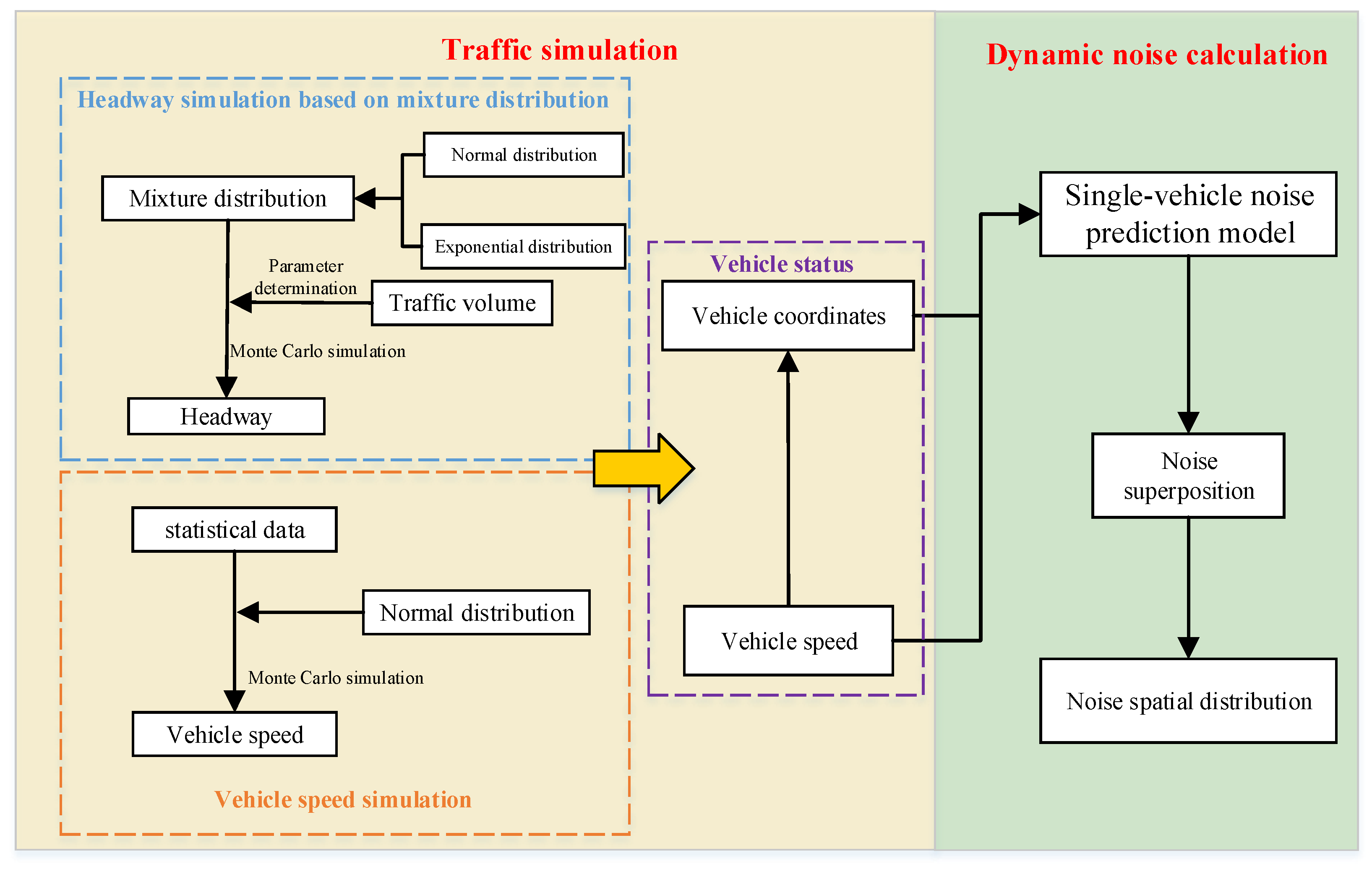
The simulation of noise spatial distribution can be divided into four steps (as shown in Figure 1): (1) Monte Carlo simulation of headway on the roadway based on a mixture distribution probability; (2) Monte Carlo simulation of vehicle speed on the roadway based on a normal distribution probability; (3) determination of vehicle states based on headway and speed; (4) calculation of noise values for individual vehicles as input, followed by noise superposition principles and receiver point arrangement to obtain noise spatial distribution.
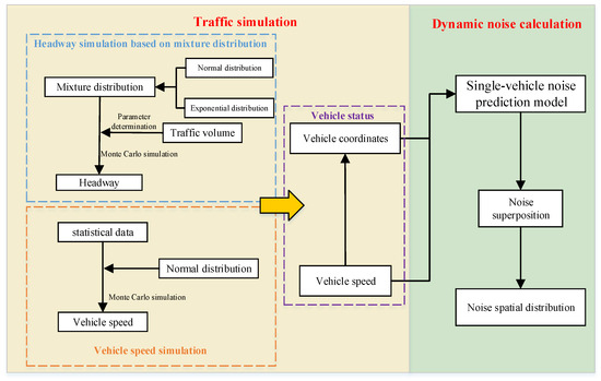
Figure 1.
Technology roadmap.
2.2. Headway Simulation Based on Mixture Distribution
Under free-driving conditions, the distribution characteristics of the headway distance are assumed to follow a negative exponential distribution, which reflects relatively independent movement patterns between vehicles. However, in the following conditions, the headway distance distribution exhibits characteristics of a normal distribution, indicating aggregated behavior influenced by dynamic interactions among vehicles.
where fmix(h) is Probability density of headway h; ω is the proportion of samples conforming to the negative exponential distribution to the total sample; λ is the reciprocal of the average frequency; µ is the expectation of the normal distribution, numerically equal to the most frequent headway in the following state; σ is Standard deviation of the normal distribution.
θ represents the set of relevant parameters (ω, µ, σ, λ) in Equation (1). i is the i-th element in the samples following a mixed distribution. fmix(h) can be simplified to a mixture distribution fi(h) composed of exponential distribution f1i and normal distribution f2i, limited by parameter θ. It can be expressed as the following:
Ii is an indicator variable corresponding to i, and Ii follows a (0, 1) distribution (as expressed by Equation (5)). And i is an unobservable random variable for it in an unknown distribution. Let g(Ii, θ) constrain the joint distribution of i and Ii, representing the probability of their simultaneous occurrence under the constraint of θ. Due to the restricted range of values that i can take, the joint distribution exists in only two cases: (1) When Ii = 1, ti follows a negative exponential distribution(f1i), and the probability of i occurring simultaneously with Ii is ωf1i; (2) When Ii = 0, i follows a normal distribution(f2i), and the probability of ti occurring simultaneously with Ii is (1 − ω)f2i. Integrating the above two cases, the joint distribution g (as Equation (6) shows) can be obtained.
The conditional probability distribution of Ii given ti is the following:
The Expectation–Maximization algorithm (EM) is simpler and more stable compared to the computationally complex maximum likelihood estimation method. Thus, a set of parameters θ (ω, µ, σ, λ) is calculated with the EM algorithm. n denotes the sample size and m denotes the number of iterations. The conditional expectation Q can be expressed by the following:
where θ(m) is the parameter at iteration m,
The parameters by maximizing the expected value function:
Using θ(m+1) as the update value for θm, repeat the steps and stop the iteration when the following conditions are met. It can be presented as the following:
Finally, by maximizing the equation and taking its partial derivatives (as expressed by Equation (12)), the four unknown parameters can be solved using four equations. Subsequently, these results are incorporated into the initial step, and through iterative processes, the final parameter estimates for the four unknowns can be obtained.
2.3. Single-Vehicle Noise Prediction Model
In the simulation of dynamic traffic flow calculation process, each vehicle on the road is treated as an independent point sound source in a semi-free sound field (as Figure 2. shown), with negligible absorption from the air and ground. Therefore, the sound value at the receiver point from the i-th second, j-th vehicle, k-th vehicle type on the road can be expressed as Equation (13) according to technical guidelines for noise impact assessment (HJ2.4-2021) [60]:
where L(i,j,k) is Noise values (dB(A)) at the receiving point in the i-th second, which generated by the j-th vehicle; L0(i,j,k) is Noise values (dB(A)) at the reference point in the i-th second, which generated by the j-th vehicle (k-th type). is Noise correction value.
where r0 is reference distance for noise propagation (r0 = 7.5 m); ri,j,k is the distance from the j-th vehicle and the k-th type of vehicle to the receiving point in the i-th second.
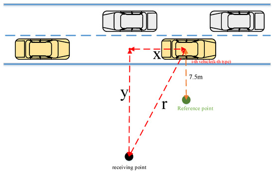
Figure 2.
Noise propagation from single vehicle.
All vehicles can be categorized into three types: large vehicles, medium vehicles, and small vehicles. Specifically, the noise calculation for each category of vehicle is as follows:
where, VS, VM, VL are speed of small vehicle, medium vehicles, large vehicles, respectively.
Then, by applying the principle of superposition of noise energy propagation, the noise value at a specific point is calculated. The noise value at the receiving point on the road from all k types of vehicles at the i-th second can be expressed by the following [60]:
The noise value Li at the receiving point from all vehicles on the road at the i-th second is as follows:
The total equivalent sound value Leq at the receiving point during the calculation time T is as follows:
3. Model Validation
According to Section 2.2, mixed distribution parameters were computed for traffic volumes ranging from 200 to 2000 (increment of 200), and the results are presented in Table 2. During the simulation, the corresponding mixture distribution parameters can be identified based on the road traffic flow.
Table 2.
Parameter values of the mixed distribution under different traffic volumes.
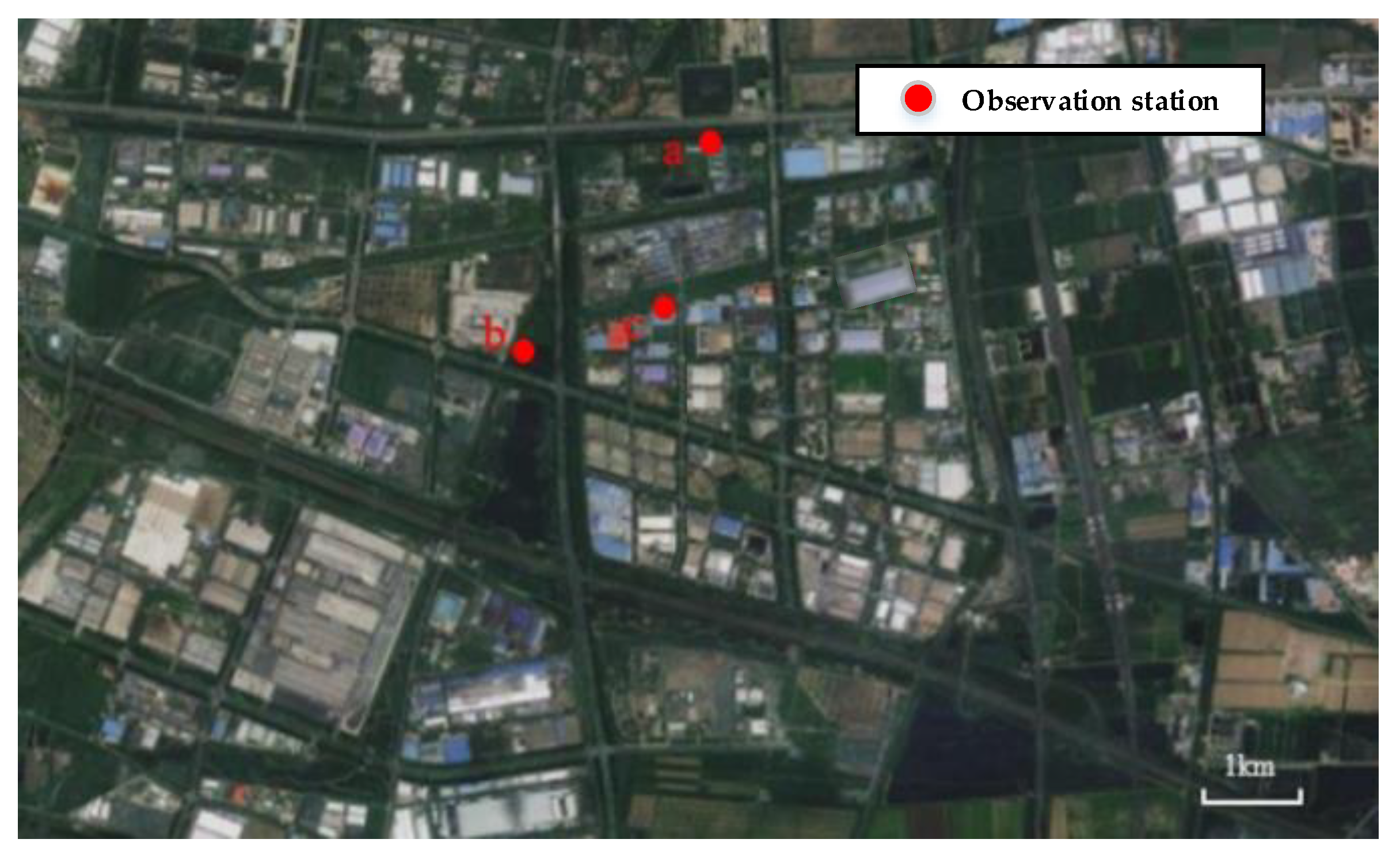
The study selected three different road values in Tianjin, including arterial roads, sub-arterial roads, and local roads (shown in Figure 3) for data collection, to verify the accuracy of the model. The survey took place on 21 July 2023, between 7:00 a.m. and 8:00 a.m.
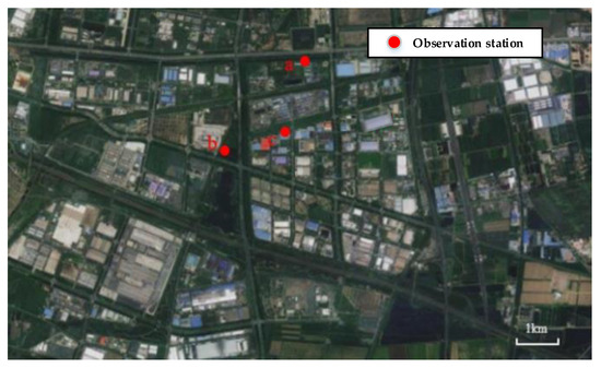
Figure 3.
Monitoring location.
The noise monitoring instrument and vehicle speedometer used are a type AWA5610 (Hangzhou Aihua Instruments Co., Ltd., Hangzhou, Zhejiang, China) integrating sound value meter and Bushnell-101911 (Bushnell Corporation, Overland Park, KS, USA), respectively. Vehicle counts were conducted manually. During the measurement period, record the number of vehicles of various types with the monitoring section as the reference. The vehicle types are listed in Table 3.
Table 3.
Small, medium, and large vehicles include vehicle types.
The data collected at monitoring points located 20 m, 60 m, and 90 m from the edge of the road are shown in Table 4. This includes corresponding monitored noise values, traffic flow rates, average traffic speeds, and simulated noise values obtained by inputting traffic flow rates into the model.
Table 4.
Monitoring data.
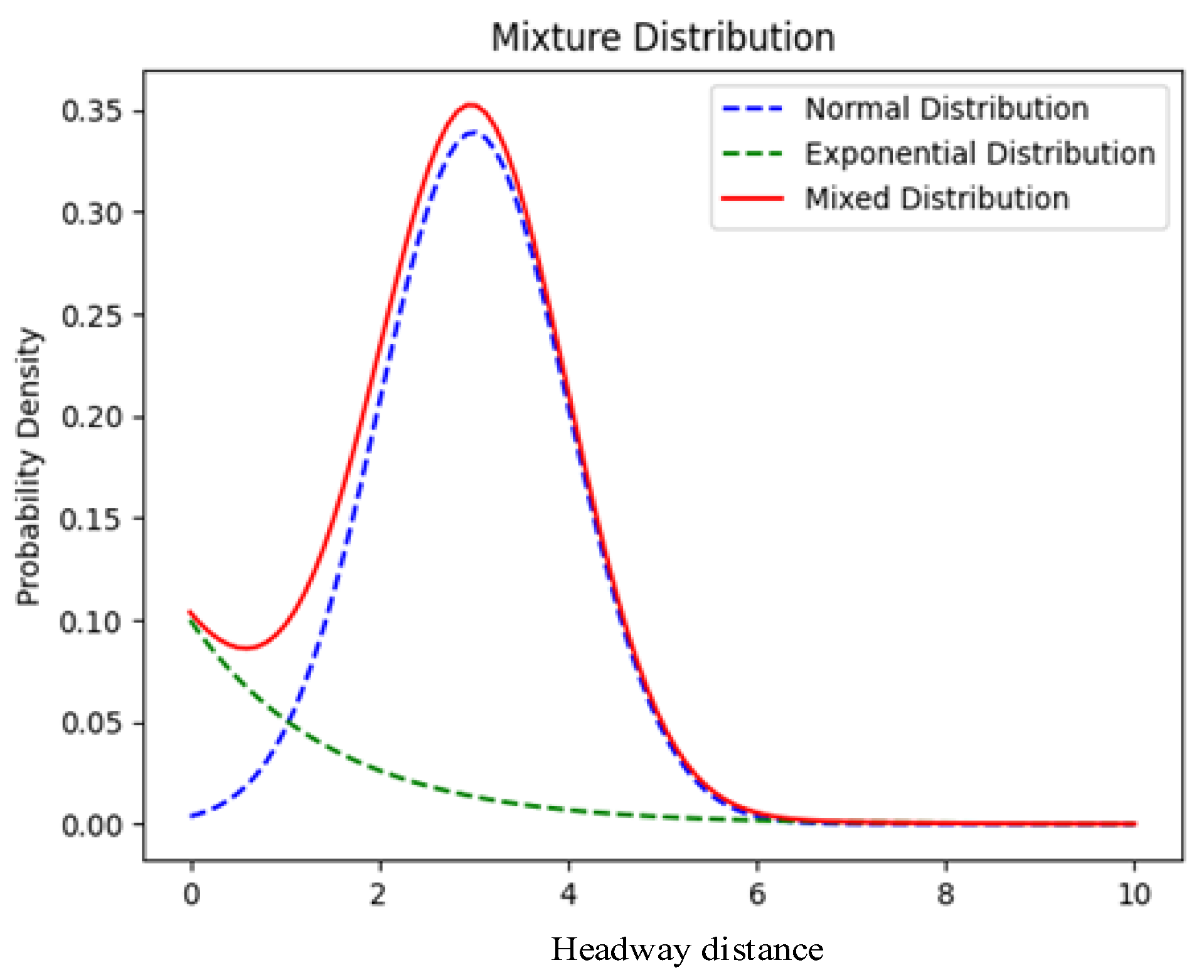
Taking point C as an example, according to the traffic flow at point C, the corresponding parameters for the mixed distribution are identified, resulting in the probability density of headways (shown in Figure 4). The minimum specified headway time is set to be greater than or equal to 2 s. The mixed-type headway time distribution curve exhibits a pattern that initially rises, then declines, and finally approaches zero, with the highest probability occurring at a headway time of 3 s, approximately 0.35. The most frequent interval in the mixed-type headway time distribution curve is between 2.5 and 4 s.
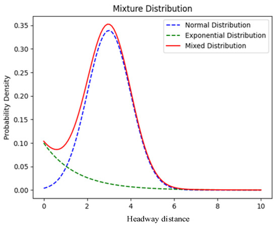
Figure 4.
Mixed distribution.
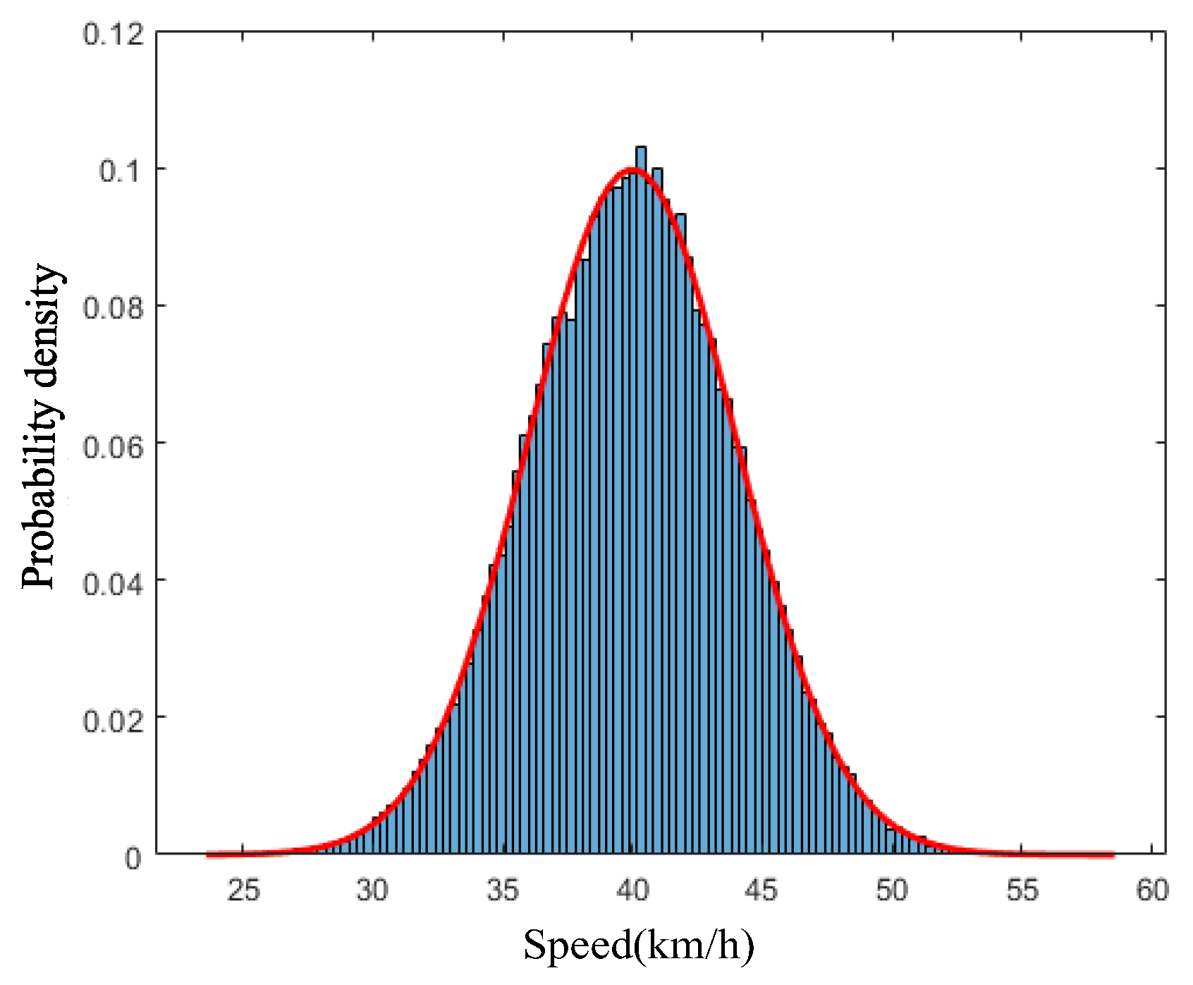
For the calculation of each vehicle’s speed, the probability of vehicle speeds is fit with a normal distribution using statistical data (results shown in Figure 5), and then assign speeds to each vehicle using Monte Carlo simulation.

Figure 5.
Probability density distribution of velocity.
The final simulation results are depicted in Figure 6. The coordinate information and travel speeds of each vehicle are obtained, followed by calculating the noise values at various reception points according to the formulas in Section 2.2.
Figure 6.
Traffic flow at point C.
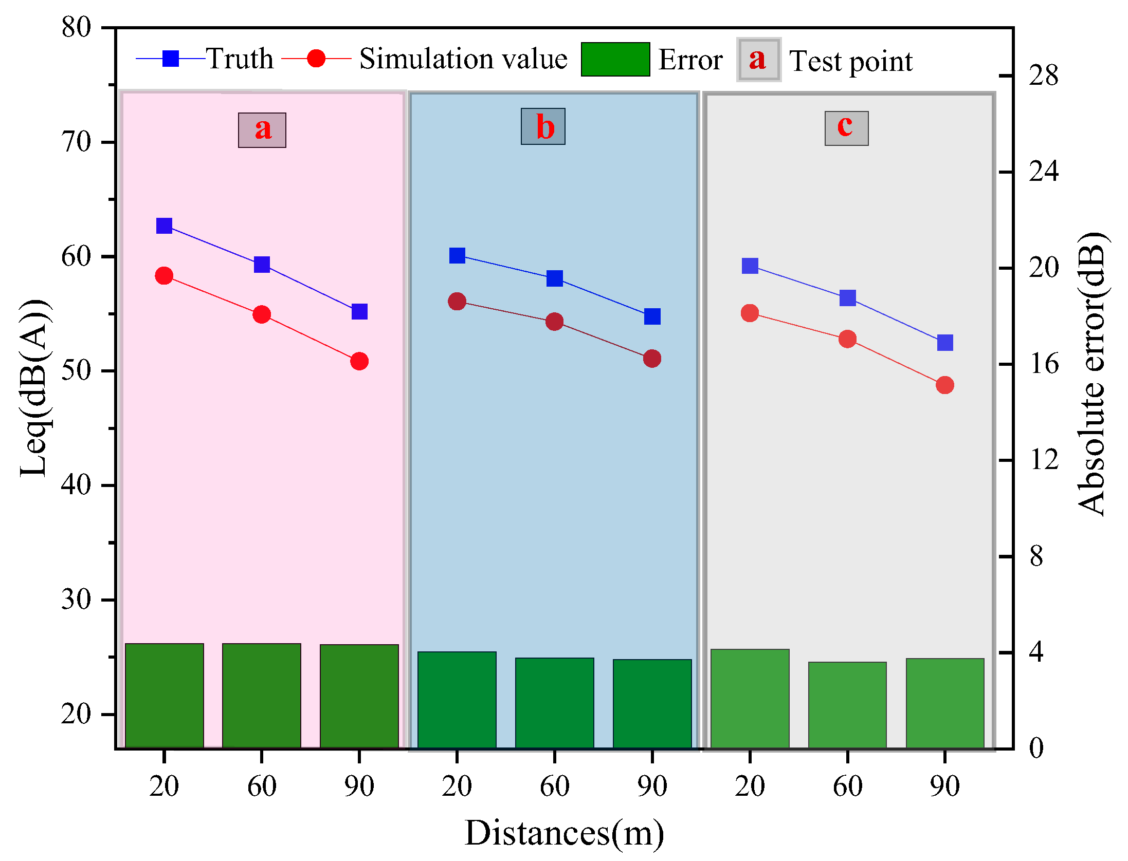
As shown in Figure 7, the validation results of the model indicate discrepancies between predicted and measured values. And absolute error (AE) (as expressed by Equation (19)) is used to assess the results. Specifically, the minimum and maximum errors are 3.6 dB(A) and 4.4 dB(A), respectively, with an average error of 4.0 dB(A). The proposed model in this study meets the accuracy requirements [28].
where vturth and vsimulation respectively are the test values and simulation values.

Figure 7.
Comparative Error.
4. Case Study
4.1. Information of Case
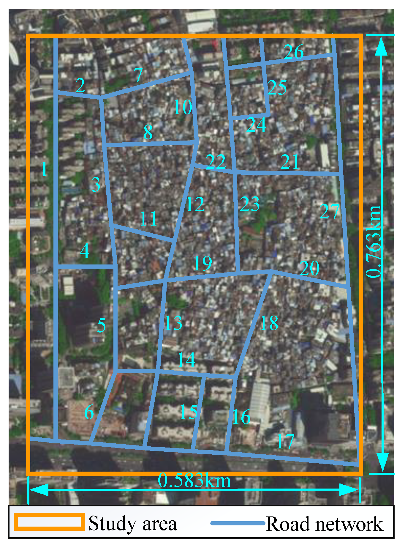
A specific district within Guangzhou, China, is selected as the study area (shown in Figure 8). To ensure comprehensive research, the study area includes a total of 27 roads across three road classifications: 3 primary roads, 17 secondary roads, and 7 tertiary roads.
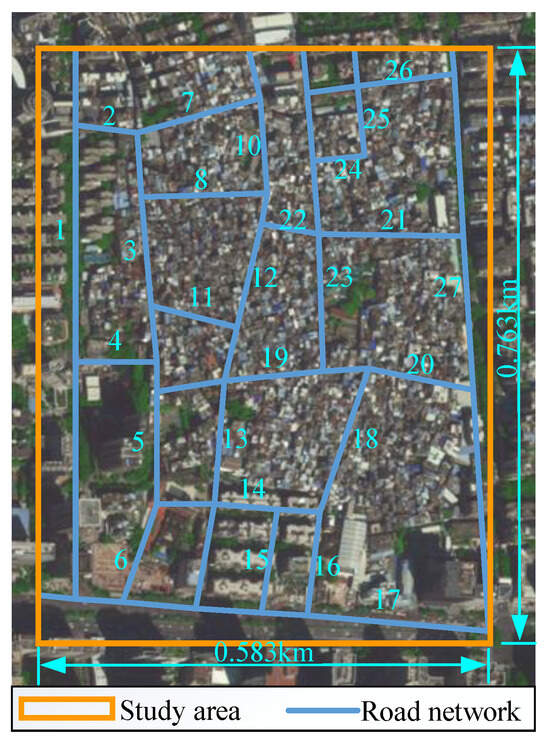
Figure 8.
Study area.
The same experimental equipment and data collection methods are utilized as shown in Section 3 to gather traffic volume and vehicle speeds for various sections of the study area during the time periods 8:15–8:30 a.m. and 8:30–8:45 a.m. The results are shown in Table 5.
Table 5.
Traffic flow and speed of road.
4.2. Analysis of Results
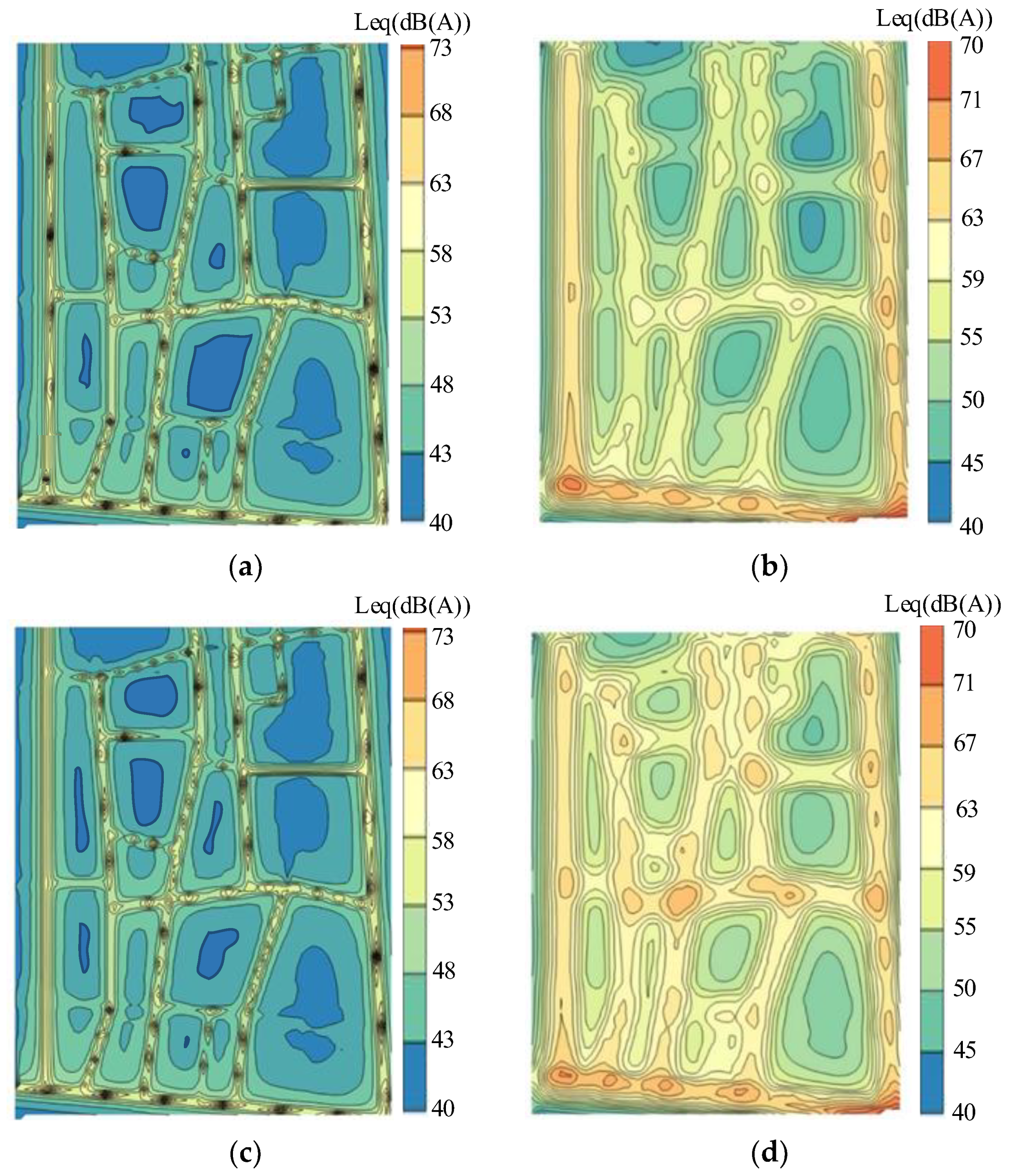
In calculating noise values in the study area using collected data, noise receivers are placed every 5 m, and noise spatial distribution maps are generated using the Kriging interpolation method. To better illustrate the spatial distribution of noise, the results with those obtained using the line source model [28] are compared. The results are shown in Figure 9. It presents that the proposed model yields more detailed results, whereas the line source model produces smoother outcomes. The line source model is a simplified model requiring fewer data. Traffic flow can be considered as a series of discrete line sources arranged at equal intervals, with each vehicle acting as an omnidirectional point source. The proposed model generally exhibits lower noise values numerically compared to the line source model, for its simulation realism and closer approximation to actual values.
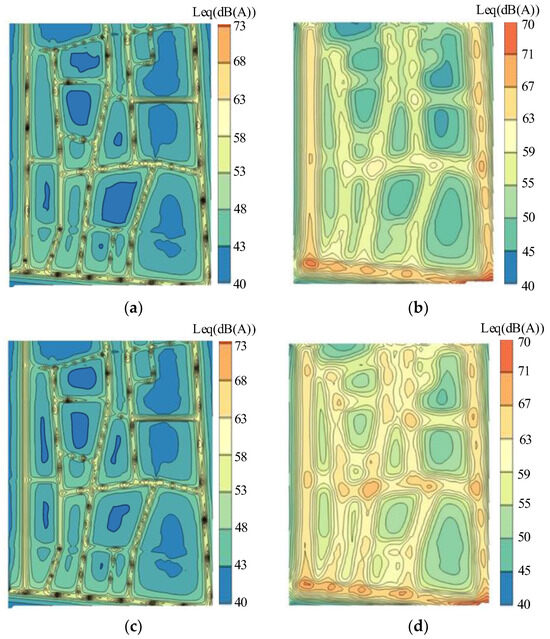
Figure 9.
Spatial Distribution of Noise: (a) Calculated by the proposed model (8:15–8:30); (b) Calculated by line source model (8:15–8:30); (c) Calculated by the proposed model (8:30–8:45); (d) Calculated by line source model (8:30–8:45).
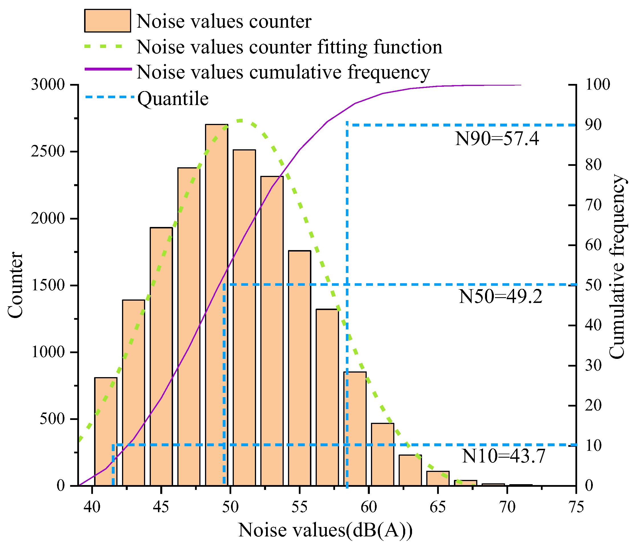
Noise values for the proposed model in the region from 8:15 to 8:30 (totaling 20,416 data) are collected. The frequency distribution of noise is shown in Figure 10. Network noise follows a normal distribution. According to the “Environmental Quality Standards for Noise” (GB 3096-2008) [61], the daytime environmental noise limit in Class II noise-sensitive areas is 60 dB(A). The frequency below the noise limit of 60 dB(A) is approximately 92.2%, indicating that some areas still do not meet the standard. The 90th percentile noise value is 57.4 dB(A), while the 50th percentile noise value is 49.2 dB(A). This indicates that although the noise values in the study area are below the allowable limit of 60 dB(A), there is not much margin left. It can be observed (Figure 9a–c) that these areas are concentrated on both sides of the road, especially alongside main roads with heavy traffic flow and high speeds.
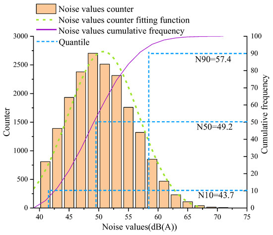
Figure 10.
Noise frequency.
5. Discussion
5.1. The Temporal Variation Pattern of Noise in Stable Traffic Flow
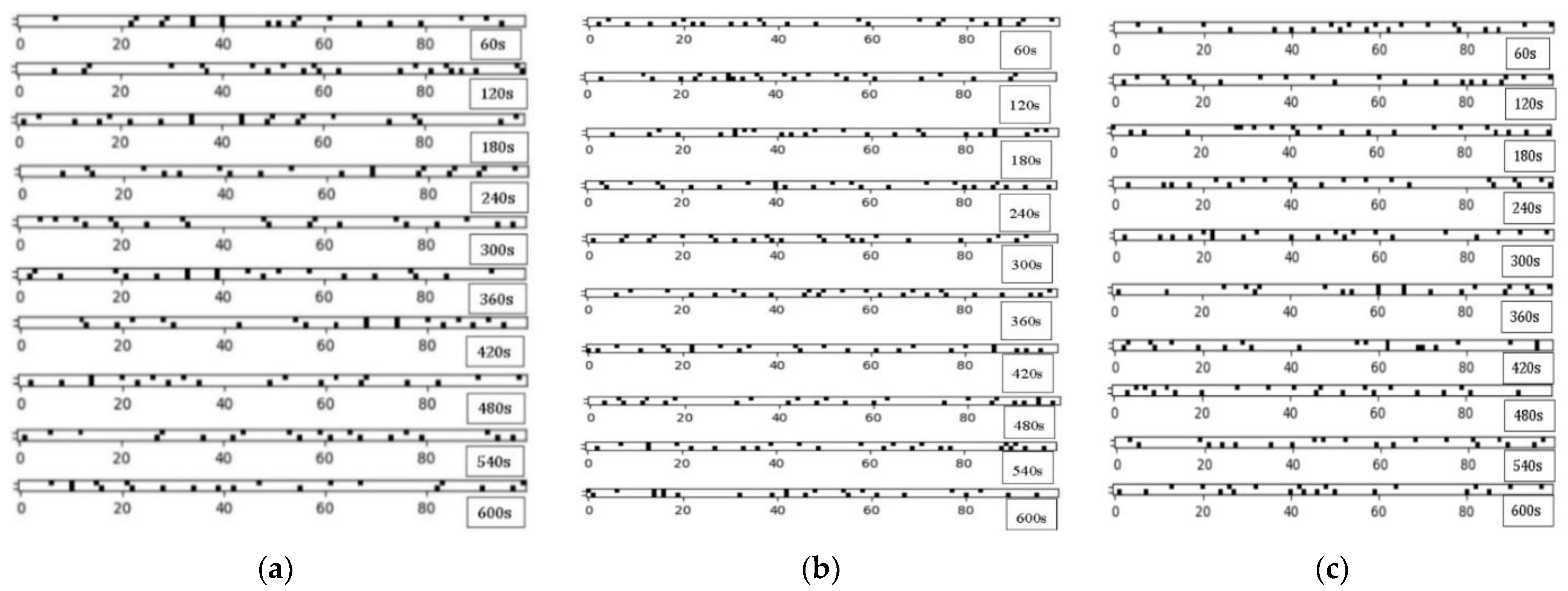
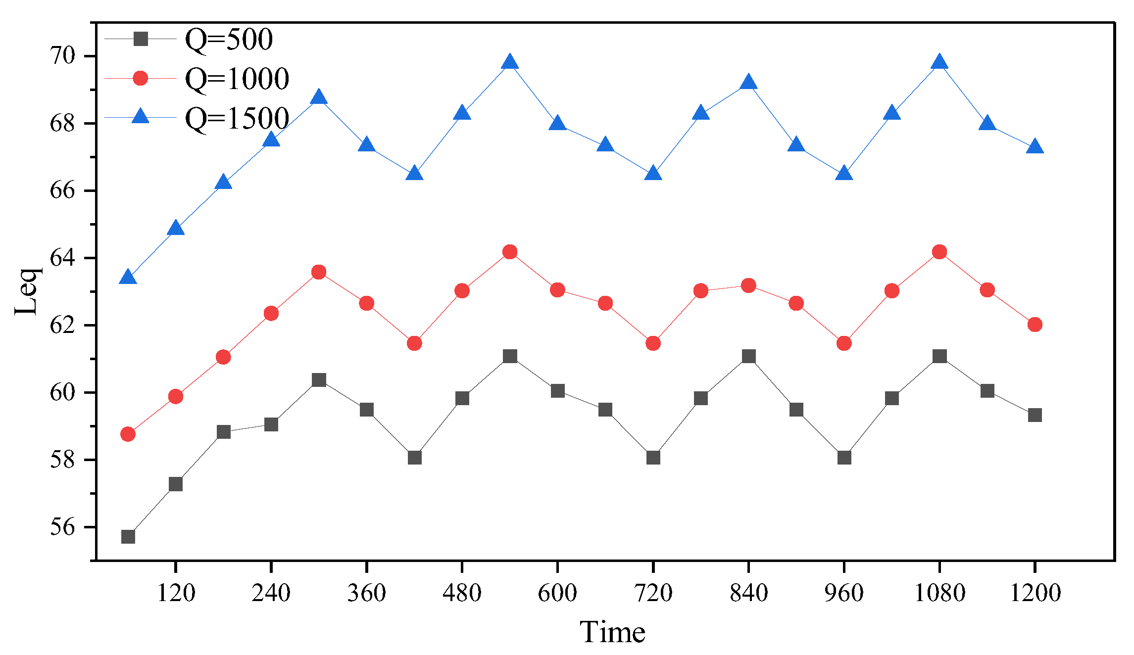
Road 27 is selected as the scene, configured as a two-way single lane, ignoring the influence of other roads. Traffic flows of 500, 1000, and 1500 were used as inputs to calculate headways, with vehicle speeds simulated by a normal distribution with a mean of 40 km/h and a standard deviation of four. Noise values were calculated every 60 s over a simulated period of 1200 s. Figure 11 depicts the traffic simulation process for the three traffic volumes (first 600 s). Noise receivers were placed 50 m from the road center to calculate noise values. As shown in Figure 12, vertically, noise values clearly increase with traffic volume. Horizontally, initially, with fewer vehicles on the road, the total noise emitted by vehicles is relatively low. As the number of vehicles increases and speeds accelerate, noise values gradually rise. Subsequently, as headways reach an optimal state under traffic flow, delay times remain within a relatively low range, maintaining smooth traffic flow and thus reducing traffic noise. However, as vehicle numbers increase again, delay times increase, resulting in higher noise values. The final noise values fluctuate around a certain value.
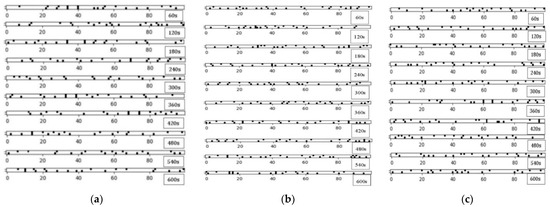
Figure 11.
Traffic simulation: (a) Q set at 500; (b) Q set at 1000; (c) Q set at 1500.
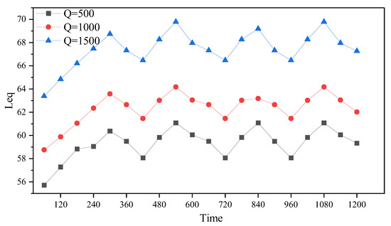
Figure 12.
Variation in noise under different traffic volumes.
5.2. The Temporal Variation Pattern of Noise in Unstable Traffic Flow
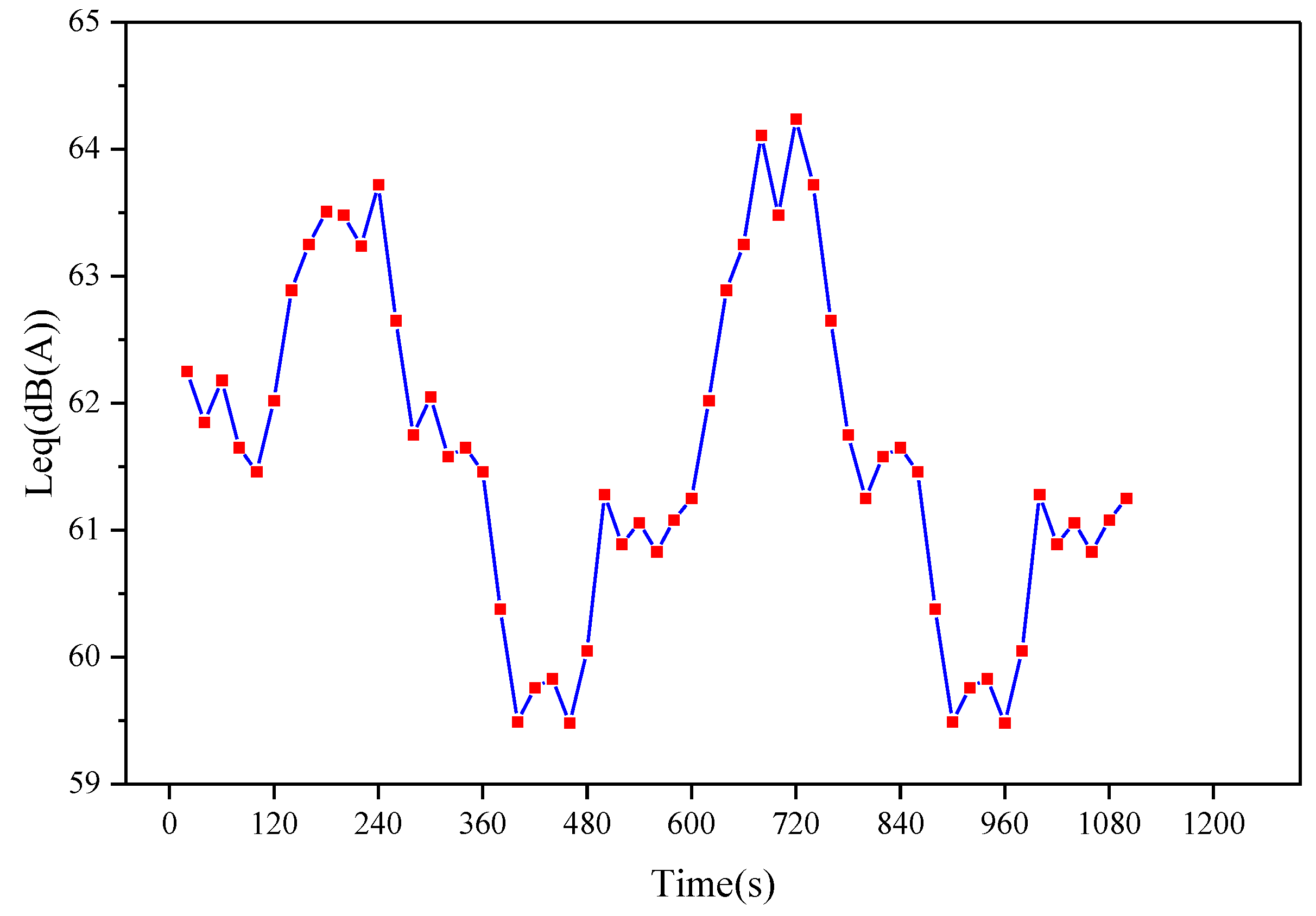
Road 27 is selected as the scene, ignoring the effects of other roads, and varied the traffic volume with a time step of 120 s (e.g., [1000, 1500, 1000, 500, 1000,1500, 1000, …...]) to simulate headways under time-varying traffic volumes. Vehicle speeds were simulated using a normal distribution with a mean of 40 km/h and a standard deviation of four. Noise values were calculated every 30 s over a total simulation period of 1100 s. The results are shown in Figure 13. It can be observed that under time-varying traffic flow, the variation in noise exhibits a step-like pattern. For instance, 120 s ago, the noise value was in a stable fluctuation state. As the traffic volume and vehicle count increased, the noise value sharply rose, followed by a fluctuating state. Subsequently, as the traffic volume decreased and vehicle count increased, the noise value sharply dropped, entering another fluctuating state.
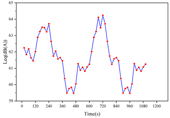
Figure 13.
The time variation in noise reception values at 50 m under different traffic flow conditions.
5.3. The Pattern of Noise Variation with Distance
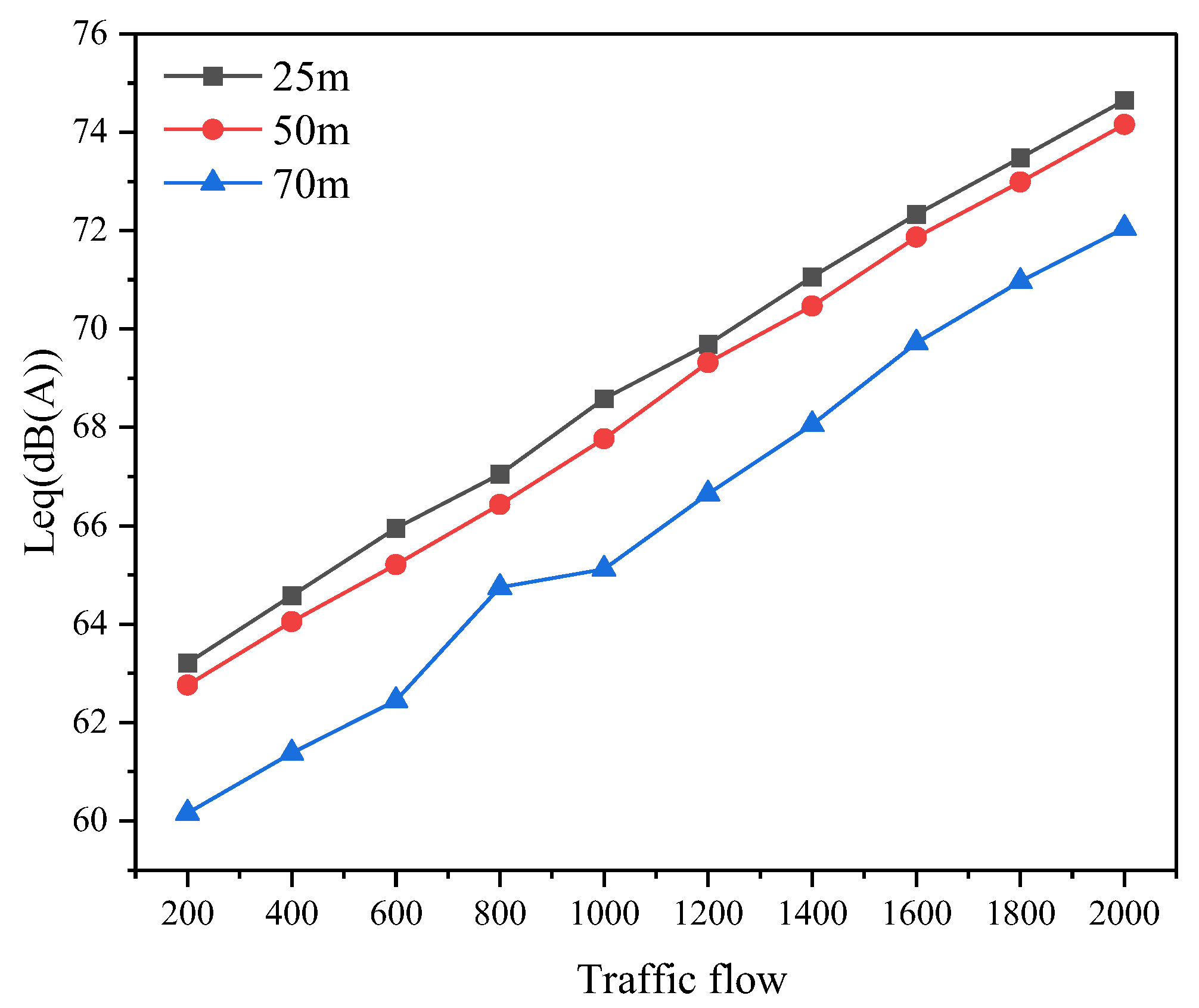
Similarly, the 27th Road is selected as the modeling scenario, with receivers positioned at distances of 25, 50, and 70 m from the midpoint of the road. Noise patterns for traffic volumes ranging from 200 to 2000 (with a step of 200) are observed, over a simulation period of 60 s. The results, shown in Figure 14, indicate that noise values increase with higher traffic volumes. Furthermore, at the same traffic volume, noise values decrease as the distance from the road increases for the receivers, with the rate of attenuation increasing with greater distances.
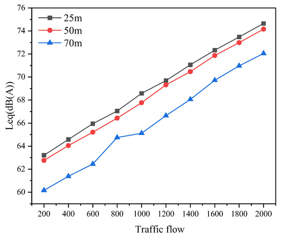
Figure 14.
Variation in noise values under stable traffic conditions.
6. Conclusions
This paper proposes a method for simulating traffic based on headway calculations using a mixed distribution, and integrates a single-vehicle noise prediction model to compute the spatial distribution of noise. The model requires traffic volume (Q) as an input parameter to determine the parameters of the mixed distribution. Through Monte Carlo simulation of headways under this mixed distribution, vehicles are dispatched. The model offers the following advantages: (a) it only requires traffic volume as an input parameter; and (b) the mixed distribution combining normal and exponential distributions is closer to reality compared to a simple normal distribution. Furthermore, experimental data testing shows that the proposed model can effectively predict noise values. The proposed method and model hold potential application value in the assessment of highway traffic noise.
Additionally, urban landscapes and the arrangement of buildings can also influence traffic noise. In this study, the effects of urban landscape and building layout were omitted. It is an aspect that needs to be addressed in future research.
Author Contributions
Conceptualization, H.W.; methodology, H.W. and Z.W.; software, Z.W. and J.C.; validation, Z.W. and J.C.; investigation, Z.W.; data curation, H.W. and J.C.; writing—original draft preparation, Z.W.; writing—review and editing, H.W. and J.C.; visualization, J.C.; supervision, J.C.; funding acquisition, H.W. All authors have read and agreed to the published version of the manuscript.
Funding
This work was supported by the Guangdong Basic and Applied Basic Research Foundation (2023A1515012482).
Institutional Review Board Statement
Not applicable.
Informed Consent Statement
Not applicable.
Data Availability Statement
The datasets used and/or analyzed during the current study are available from the corresponding author upon reasonable request.
Conflicts of Interest
The authors declare no conflicts of interest.
References
- Ministry of Ecology and Environment of the People’s Republic of China. China Environmental Noise Prevention and Control Annual Report 2020; Ministry of Ecology and Environment of the People’s Republic of China: Beijing, China, 2020. [Google Scholar]
- Tong, H.; Kang, J. Relationships between Noise Complaints and Socio-Economic Factors in England. Sustain. Cities Soc. 2021, 65, 102573. [Google Scholar] [CrossRef]
- World Health Organization. Environment Noise Guidelines for the European Region. Available online: https://www.who.int/europe/publications/i/item/9789289053563 (accessed on 14 February 2023).
- Guski, R.; Schreckenberg, D.; Schuemer, R. WHO environmental noise guidelines for the european region: A systematic review on environmental noise and annoyance. Int. J. Environ. Res. Public Health 2017, 14, 1539. [Google Scholar] [CrossRef] [PubMed]
- Kempen, E.; Casas, M.; Pershagen, G.; Foraster, M. WHO environmental noise guidelines for the european region: A systematic review on environmental noise and cardiovascular and metabolic effects: A summary. Int. J. Environ. Res. Public Health 2018, 15, 397. [Google Scholar] [CrossRef] [PubMed]
- Thacher, J.D.; Poulsen, A.H.; Raaschou-Nielsen, O.; Hvidtfeldt, U.A.; Brandt, J.; Christensen, J.H.; Khan, J.; Levin, G.; Münzel, T.; Sørensen, M. Exposure to Transportation Noise and Risk for Cardiovascular Disease in a Nationwide Cohort Study from Denmark. Environ. Res. 2022, 211, 113106. [Google Scholar] [CrossRef] [PubMed]
- Wang, H.; Yan, X.; Chen, J.; Cai, M. Urban Noise Exposure Assessment Based on Principal Component Analysis of Points of Interest. Environ. Pollut. 2024, 342, 123134. [Google Scholar] [CrossRef] [PubMed]
- Vukić, L.; Mihanović, V.; Fredianelli, L.; Plazibat, V. Seafarers’ Perception and Attitudes towards Noise Emission on Board Ships. Int. J. Environ. Res. Public Health 2021, 18, 6671. [Google Scholar] [CrossRef]
- Muzet, A. Environmental Noise, Sleep and Health. Sleep Med. Rev. 2007, 11, 135–142. [Google Scholar] [CrossRef]
- Fredianelli, L.; Carpita, S.; Licitra, G. A Procedure for Deriving Wind Turbine Noise Limits by Taking into Account Annoyance. Sci. Total Environ. 2019, 648, 728–736. [Google Scholar] [CrossRef]
- Erickson, L.C.; Newman, R.S. Influences of Background Noise on Infants and Children. Curr. Dir. Psychol. Sci. 2017, 26, 451–457. [Google Scholar] [CrossRef]
- Leon Bluhm, G.; Berglind, N.; Nordling, E.; Rosenlund, M. Road Traffic Noise and Hypertension. Occup. Environ.-Ment. Med. 2006, 64, 122–126. [Google Scholar] [CrossRef]
- Dratva, J.; Phuleria, H.C.; Foraster, M.; Gaspoz, J.-M.; Keidel, D.; Künzli, N.; Liu, L.-J.S.; Pons, M.; Zemp, E.; Gerbase, M.W.; et al. Transportation Noise and Blood Pressure in a Population-Based Sample of Adults. Environ. Health Perspect. 2012, 120, 50–55. [Google Scholar] [CrossRef]
- Petri, D.; Licitra, G.; Vigotti, M.A.; Fredianelli, L. Effects of Exposure to Road, Railway, Airport and Recreational Noise on Blood Pressure and Hypertension. Int. J. Environ. Res. Public Health 2021, 18, 9145. [Google Scholar] [CrossRef]
- Marquis-Favre, C.; Braga, R.; Gourdon, E.; Combe, C.; Gille, L.-A.; Ribeiro, C.; Mietlicki, F. Estimation of Psychoacoustic and Noise Indices from the Sound Pressure Level of Transportation Noise Sources: Investigation of Their Potential Benefit to the Prediction of Long-Term Noise Annoyance. Appl. Acoust. 2023, 211, 109560. [Google Scholar] [CrossRef]
- Lavandier, C.; Regragui, M.; Dedieu, R.; Royer, C.; Can, A. Influence of Road Traffic Noise Peaks on Reading Task Performance and Disturbance in a Laboratory Context. Acta Acust. 2022, 6, 3. [Google Scholar] [CrossRef]
- Huth, C.; Forstreuter, M.; Arlt, R.; Liepert, M. Annoyance at the Point of Emission versus Immission for Impulsive Noises at Train Passings. J. Acoust. Soc. Am. 2020, 148, 2567. [Google Scholar] [CrossRef]
- Licitra, G.; Bolognese, M.; Chiari, C.; Carpita, S.; Fredianelli, L. Noise Source Predominance Map: A New Representation for Strategic Noise Maps. Noise Mapp. 2022, 9, 269–279. [Google Scholar] [CrossRef]
- Bolognese, M.; Fredianelli, L.; Stasi, G.; Ascari, E.; Crifaci, G.; Licitra, G. Citizens’ Exposure to Predominant Noise Sources in Agglomerations. Noise Mapp. 2024, 11, 20240007. [Google Scholar] [CrossRef]
- Ramos-Romero, C.; Asensio, C.; Moreno, R.; de Arcas, G. Urban Road Surface Discrimination by Tire-Road Noise Analysis and Data Clustering. Sensors 2022, 22, 9686. [Google Scholar] [CrossRef]
- Del Pizzo, A.; Teti, L.; Moro, A.; Bianco, F.; Fredianelli, L.; Licitra, G. Influence of Texture on Tyre Road Noise Spectra in Rubberized Pavements. Appl. Acoust. 2020, 159, 107080. [Google Scholar] [CrossRef]
- de León, G.; Del Pizzo, A.; Teti, L.; Moro, A.; Bianco, F.; Fredianelli, L.; Licitra, G. Evaluation of Tyre/Road Noise and Texture Interaction on Rubberised and Conventional Pavements Using CPX and Profiling Measurements. Road Mater. Pavement Des. 2020, 21, S91–S102. [Google Scholar] [CrossRef]
- Karbalaei, S.; Karimi, E.; Naji, H.; Ghasempoori, S.; Hosseini, S.; Abdollahi, M. Investigation of the traffic noise attenuation provided by roadside green belts. Fluct. Noise Lett. 2015, 14, 1550036. [Google Scholar] [CrossRef]
- Ow, L.; Ghosh, S. Urban cities and road traffic noise: Reduction through vegetation. Appl. Acoust. 2017, 120, 15–20. [Google Scholar] [CrossRef]
- Ilgurel, N.; Akdag, N.; Akdag, A. Evaluation of noise exposure before and after noise barriers, a simulation study in Istanbul. Environ. Eng. Manag. J. 2016, 24, 293–302. [Google Scholar] [CrossRef]
- Wang, H.; Wu, Z.; Wu, Z.; Hou, Q. Urban Network Noise Control Based on Road Grade Optimization Considering Comprehensive Traffic Environment Benefit. J. Environ. Manag. 2024, 364, 121451. [Google Scholar] [CrossRef]
- Liu, Y.; Ma, X.; Shu, L.; Yang, Q.; Zhang, Y.; Huo, Z.; Zhou, Z. Internet of Things for Noise Mapping in Smart Cities: State of the Art and Future Directions. IEEE Netw. 2020, 34, 112–118. [Google Scholar] [CrossRef]
- Wang, H.; Sun, B.; Chen, L. An Optimization Model for Planning Road Networks That Considers Traffic Noise Impact. Appl. Acoust. 2022, 192, 108693. [Google Scholar] [CrossRef]
- Yan, X.; Wu, Z.; Wang, H. Network Noise Control under Speed Limit Strategies Using an Improved Bilevel Programming Model. Transp. Res. Part D Transp. Environ. 2023, 121, 103805. [Google Scholar] [CrossRef]
- Wang, H.; Wu, Z.; Chen, J.; Chen, L. Evaluation of Road Traffic Noise Exposure Considering Differential Crowd Characteristics. Transp. Res. Part D Transp. Environ. 2022, 105, 103250. [Google Scholar] [CrossRef]
- Sun, B.; Wang, H.; Hu, L.; Zhang, Q.; Shi, H.; Mao, H. Exploring Vehicle-Centric Strategies for Sustainable Urban Mobility: A Theoretical Framework for Saving Energy and Reducing Noise in Transportation. J. Environ. Manag. 2024, 358, 120798. [Google Scholar] [CrossRef]
- Licitra, G.; Artuso, F.; Bernardini, M.; Moro, A.; Fidecaro, F.; Fredianelli, L. Acoustic Beamforming Algorithms and Their Applications in Environmental Noise. Curr. Pollut. Rep. 2023, 9, 486–509. [Google Scholar] [CrossRef]
- Licitra, G.; Di Marco, B.; Ricardo, M.; Francesco, B.; De Luca, F. CNOSSOS-EU Coefficients for Electric Vehicle Noise Emission. Appl. Acoust. 2023, 211, 109511. [Google Scholar] [CrossRef]
- Bolognese, M.; Carpita, S.; Fredianelli, L.; Licitra, G. Definition of Key Performance Indicators for Noise Monitoring Networks. Environments 2023, 10, 61. [Google Scholar] [CrossRef]
- Shah, S.K.; Tariq, Z.; Lee, J.; Lee, Y. Real-Time Machine Learning for Air Quality and Environmental Noise Detection. In Proceedings of the 2020 IEEE International Conference on Big Data (Big Data), Atlanta, GA, USA, 10–13 December 2020. [Google Scholar]
- Moreno, R.; Bianco, F.; Carpita, S.; Monticelli, A.; Fredianelli, L.; Licitra, G. Adjusted Controlled Pass-by (CPB) Method for Urban Road Traffic Noise Assessment. Sustainability 2023, 15, 5340. [Google Scholar] [CrossRef]
- Li, F.; Liao, S.S.; Cai, M. A New Probability Statistical Model for Traffic Noise Prediction on Free Flow Roads and Control Flow Roads. Transp. Res. Part D Transp. Environ. 2016, 49, 313–322. [Google Scholar] [CrossRef]
- Stylianos, K.; Marco, P. Common Noise Assessment Methods for Europe (CNOSSOS-EU): Implementation Challenges in the Context of EU Noise Policy Developments and Future Perspectives. In Proceedings of the 23rd Congress on Sound and Vibration, Athens, Greece, 10–14 July 2016. [Google Scholar]
- Givargis, S.; Mahmoodi, M. Converting the UK Calculation of Road Traffic Noise (CORTN) to a Model Capable of Calculating LAeq,1h for the Tehran’s Roads. Appl. Acoust. 2008, 69, 1108–1113. [Google Scholar] [CrossRef]
- Sakamoto, S. Road Traffic Noise Prediction Model “ASJ RTN-Model 2018’’: Report of the Research Committee on Road Traffic Noise. Acoust. Sci. Technol. 2020, 41, 529–589. [Google Scholar] [CrossRef]
- Du, C.; Qiu, X.; Li, F.; Cai, M. A Simulation of Traffic Noise Emissions at a Roundabout Based on a Cellular Automaton Model. Acta Acust. 2021, 5, 42. [Google Scholar] [CrossRef]
- Li, F.; Lin, Y.; Cai, M.; Du, C. Dynamic Simulation and Characteristics Analysis of Traffic Noise at Roundabout and Signalized Intersections. Appl. Acoust. 2017, 121, 14–24. [Google Scholar] [CrossRef]
- Estévez-Mauriz, L.; Forssén, J. Dynamic Traffic Noise Assessment Tool: A Comparative Study between a Roundabout and a Signalised Intersection. Appl. Acoust. 2018, 130, 71–86. [Google Scholar] [CrossRef]
- Yan, X.; Wu, Z.; Wu, Z.; Wang, H. Study on the Network Acoustics Environment Effects of Traffic Management Measures by a Bilevel Programming Model. Sustain. Cities Soc. 2024, 101, 105203. [Google Scholar] [CrossRef]
- Li, F.; Lai, R.; Rong, Y.; Yu, F.; Du, C.; Lan, Z.; Ye, B.; Li, Z. Dynamic Traffic Noise Simulation at Signal-Controlled Intersections Based on Cellular Automata Model. Appl. Acoust. 2024, 224, 110128. [Google Scholar] [CrossRef]
- Hou, G.; Chen, S.; Bao, Y. Development of Travel Time Functions for Disrupted Urban Arterials with Microscopic Traffic Simulation. Phys. A 2022, 593, 126961. [Google Scholar] [CrossRef]
- Li, F.; Xue, W.; Rong, Y.; Du, C.; Tang, J.; Zhao, Y. A Probability Distribution Prediction Method for Expressway Traffic Noise. Transp. Res. Part D Transp. Environ. 2022, 103, 103175. [Google Scholar] [CrossRef]
- Baclet, S.; Khoshkhah, K.; Pourmoradnasseri, M.; Rumpler, R.; Hadachi, A. Near-Real-Time Dynamic Noise Mapping and Exposure Assessment Using Calibrated Microscopic Traffic Simulations. Transp. Res. Part D Transp. Environ. 2023, 124, 103922. [Google Scholar] [CrossRef]
- Eisele, W.L.; Toycen, C.M. Identifying and Quantifying Operational and Safety Performance Measures for Access Management: Micro-Simulation Results; Texas Transportation Institute, The Texas A&M University System: College Station, TX, USA, 2005. [Google Scholar]
- Al-Fuqaha, A.; Guizani, M.; Mohammadi, M.; Aledhari, M.; Ayyash, M. Internet of Things: A Survey on Enabling Technologies, Protocols, and Applications. IEEE Commun. Surv. Tutor. 2015, 17, 2347–2376. [Google Scholar] [CrossRef]
- Ambros, J.; Turek, R.; Paukrt, J. Road Safety Evaluation Using Traffic Conflicts: Pilot Comparison of Micro-Simulation and Observation. In Proceedings of the Second International Conference on Traffic and Transport Engineering (ICTTE), Belgrade, Serbia, 27–28 November 2014. [Google Scholar]
- Yang, H. Simulation-based evaluation of traffic safety performance using surrogate safety measures. Ph.D. Thesis, Rutgers, The State University of New Jersey, New Brunswick, NJ, USA, 2012. [Google Scholar]
- Caliendo, C.; Guida, M. Microsimulation Approach for Predicting Crashes at Unsignalized Intersections Using Traffic Conflicts. J. Transp. Eng. 2012, 138, 1453–1467. [Google Scholar] [CrossRef]
- Dalla Chiara, B.; Deflorio, F.; Diwan, S. Assessing the Effects of Inter-Vehicle Communication Systems on Road Safety. IET Intell. Transp. Syst. 2009, 3, 225. [Google Scholar] [CrossRef]
- Yang, S.; Du, M.; Chen, Q. Impact of Connected and Autonomous Vehicles on Traffic Efficiency and Safety of an On-Ramp. Simul. Model. Pract. Theory 2021, 113, 102374. [Google Scholar] [CrossRef]
- Brügmann, J.; Schreckenberg, M.; Luther, W. A Verifiable Simulation Model for Real-World Microscopic Traffic Simulations. Simul. Model. Pract. Theory 2014, 48, 58–92. [Google Scholar] [CrossRef]
- Nygren, J.; Boij, S.; Rumpler, R.; O’Reilly, C.J. Vehicle-Specific Noise Exposure Cost: Noise Impact Allocation Methodology for Microscopic Traffic Simulations. Transp. Res. Part D Transp. Environ. 2023, 118, 103712. [Google Scholar] [CrossRef]
- Can, A.; Aumond, P. Estimation of Road Traffic Noise Emissions: The Influence of Speed and Acceleration. Transp. Res. Part D Transp. Environ. 2018, 58, 155–171. [Google Scholar] [CrossRef]
- Saha, P.; Roy, R.; Sarkar, A.K.; Pal, M. Preferred Time Headway of Drivers on Two-Lane Highways with Heterogeneous Traffic. Transp. Lett. 2017, 11, 200–207. [Google Scholar] [CrossRef]
- HJ2.4-2021; Technical Guidelines for Noise Impact Assessment. Ministry of Ecology and Environment of the People’s Republic of China: Beijing, China, 2021.
- GB 3096–2008; Environmental Quality Standard for Noise. China’s State Environmental Protection Administration: Beijing, China, 2008.


Disclaimer/Publisher’s Note: The statements, opinions and data contained in all publications are solely those of the individual author(s) and contributor(s) and not of MDPI and/or the editor(s). MDPI and/or the editor(s) disclaim responsibility for any injury to people or property resulting from any ideas, methods, instructions or products referred to in the content. |
© 2024 by the authors. Licensee MDPI, Basel, Switzerland. This article is an open access article distributed under the terms and conditions of the Creative Commons Attribution (CC BY) license (https://creativecommons.org/licenses/by/4.0/).