A Dynamic Approach to Sustainable Knitted Footwear Production in Industry 4.0: Integrating Short-Term Profitability and Long-Term Carbon Efficiency

Abstract

This study proposes a novel approach to support sustainable decision-making in knitted shoe manufacturing by integrating activity-based costing (ABC), the theory of constraints (TOC), and carbon emission costs into a comprehensive mathematical programming model. The model is applied to evaluate the impact of different carbon tax and carbon trading policies on the profitability and product mix of a knitted shoe company in Taiwan. The model considers single-period and multi-period scenarios, as well as continuous and discontinuous carbon tax functions, with and without carbon trading. The results show that a continuous carbon tax leads to higher profitability in single-period models, while a continuous carbon tax function combined with carbon trading yields the highest profits in multi-period models. Reducing the carbon emission cap is found to be more effective in curbing emissions than raising carbon taxes. This research contributes to sustainable operations management by providing a holistic approach that integrates cost control, profit optimization, and environmental sustainability in the context of Industry 4.0. The findings offer valuable insights for footwear manufacturers in making strategic decisions and for governments in designing effective carbon tax and emission trading schemes to drive industrial transformation towards a low-carbon economy.

1. Introduction

Research Background and Motivation

Given the heightened governmental regulations and increasing societal focus on environmental stewardship, environmental considerations have become pivotal to corporate agendas. The shoe manufacturing sector, in particular, faces significant environmental challenges because of its production processes, sourcing of materials, and the harmful effects of organic compounds and solvents on its workforce [1]. Such a transformation, including the adoption of eco-friendly products, is crucial for maintaining a competitive edge. The Ellen MacArthur Foundation [2] highlights the inefficiency and pollution rampant in the current life cycle of clothing, warning of dire global impacts if the trend persists. Addressing the fashion industry’s sustainability challenges necessitates a holistic view that encompasses the entire supply chain [3].

Studies focusing on the footwear industry have promoted environmental sustainability concepts. Using carbon fiber prepreg scraps for toe caps provides a sustainable, lightweight alternative with a lower environmental impact compared with traditional materials [4]. Additionally, innovations like Design for Additive Manufacturing (DfAM) and Design for Assembly (DfD) reduce the fashion industry’s carbon footprint. An optimized shoe design using Polyamide 12 and TPU with a snapfit assembly cuts mass by 34% and enhances sustainability [5].

Caniato et al. [6] identified key factors and practices for international brands aiming to enhance environmental sustainability. Other research has delved into the possibilities for recycling and remanufacturing at the end-of-life stage of footwear products [7,8].

The tanning sector, crucial to the leather footwear supply chain, has also been a focus of study. Bhavan et al. [9] developed a new tanning method to lessen the chemical load in tannery wastewater. Chen et al. [10] investigated the carbon footprint of producing aniline leather, while Kılıç et al. [11] calculated the carbon footprint of a Turkish tannery, pinpointing major impact sources. Milà I Canals et al. [12] employed life cycle assessment (LCA) to identify significant environmental impacts in chrome-tanned leather production, leading to the proposition of environmental labels for leather goods. As indicated in recent studies, such as Daddi et al. [13], the key to reducing carbon emissions in the life cycle of shoe manufacturing is to improve the efficiency of component manufacturing and to select more environmentally friendly raw materials. By optimizing manufacturing processes and material choices, the carbon footprint of shoes can be significantly reduced, achieving the goal of carbon reduction.

Early research by Perdijk et al. [14] proposed eco-labeling for footwear, laying the groundwork for further study. The article found that leather footwear materials have the most significant environmental impact during their life cycle and pointed out that there is currently limited research on thermochemical treatments, especially pyrolysis, as a footwear waste recycling option. The article proposed to further investigate pyrolysis as a potential footwear waste recycling method to reduce waste streams in landfills [15]. Other assessments have oversimplified material modeling or focused on specific footwear types, making some findings less reliable [16].

The motivation for this study is the urgent need to address the environmental impact of the footwear industry. With increasing regulatory standards and heightened consumer awareness of environmental issues, the industry faces pressure to adopt sustainable practices. By integrating advanced cost management techniques and carbon emission analysis, this study aims to provide actionable insights to help manufacturers enhance both profitability and environmental performance. This dual focus on economic and ecological outcomes drives the exploration of innovative solutions applicable to various industrial scenarios.

Efficient waste management is essential for environmental sustainability, yet it is challenged by the rise in waste due to technological progress, improved living standards, and changing consumer behaviors [17,18,19,20]. Although textiles, including footwear, constitute only about 7% of household waste [21], the environmental impact of shoe waste is significant because of the toxic materials used in their production [16,22,23]. Global footwear production in 2022 reached 23.9 billion pairs, recovering to pre-pandemic levels with a growth of 7.6% [24]. This reflects increased consumer consumption, which, along with socio-economic advancements, contributes to both economic gains and environmental strains, such as increased waste and pollution [1,25,26]. To address these challenges, the industry is exploring innovations such as knitted materials for shoe uppers and sustainable production methods. These innovations aim to mitigate environmental impacts and take advantage of market shifts towards sustainability.

The process of this research is divided into the following five sections:

(1)

Section 1, Introduction: This section explains the research background and motivation of this research.

(2)

Section 2, Literature: This section mainly discusses the impact and transformation of the footwear industry on the environment, carbon tax and carbon rights, and the combination of the constraint theory of the activity-based cost system.

(3)

Section 3, Research Design and Methods: This section defines the single-period model, multi-period model, and model parameter data hypothesis.

(4)

Section 4, Research Results and Analysis: This section describes the model results and model analysis.

(5)

Section 5, Discussion and Conclusions: This section describes the research conclusions and research limitations.

2. Literature

2.1. Carbon Emissions, Carbon Taxes, Carbon Rights

The literature on the EU Emissions Trading System (EU ETS) finds no widespread effects on competitiveness or significant carbon leakage. However, the findings are mainly from the first two trading periods, show some heterogeneity without clear patterns, and lack long-term impact studies. Additionally, China’s carbon trading system, exemplified by platforms such as the Shanghai Environment and Energy Exchange, provides a compelling case study [27,28]. This suggests a pathway for Taiwan to become a crucial carbon trading center in Asia if it can align with international standards [29].

However, the integration of the footwear industry into carbon trading markets has been minimal in some major Asian economies, presenting both a unique challenge and an opportunity to reduce its environmental impact through incentivized sustainable practices. The examination of low-carbon innovation highlights the importance of governmental support in stimulating low-carbon innovation systems. Despite the absence of an established energy or carbon tax, energy transition policies in some countries have been exploring such proposals. For instance, carbon trading systems exemplified by platforms such as the Shanghai Environment and Energy Exchange suggest a pathway for Taiwan to become a crucial carbon trading center in Asia if it aligns with international standards. This perspective is reinforced by several studies on low-carbon innovation and the critical role of governmental support in fostering such systems [30,31,32,33,34,35,36].

2.2. The Relationship among Activity-Based Costing, Constraint Theory, and Industry 4.0

Luthra and Mangla [37] identify Industry 4.0 and sustainability as keys to boosting organizational efficiency and promoting eco-friendly manufacturing. Kiel et al. [38] discuss how Industry 4.0’s advanced tools address global market challenges, enhancing customization and innovation speed. Dalenogare et al. [39] note its benefits in improving production efficiency and reducing costs. Gabriel and Pessl [40] and Müller et al. [41] explore its environmental and social sustainability impacts, highlighting waste reduction and improved workplace safety, while acknowledging challenges like data management and electronic waste. Industry 4.0’s integration with sustainability, particularly in the circular economy, is explored by de Sousa Jabbour et al. [42], with a comprehensive review by Beltrami and Orzes [43]. This technological shift, as Park et al. [44] suggest, aligns with firms adopting sustainability practices under the pressure of stakeholder expectations, moving beyond profit towards environmental and social stewardship. The development of activity-based costing (ABC) by Cooper and Kaplan [45] revolutionized cost management, enabling precise cost allocation and environmental sustainability insights [46,47]. The United Nations’ emphasis on environmental cost management further highlights ABC’s importance in sustainable strategy development [48]. The theory of constraints (TOC) by Goldratt and Cox [49] complements this by enhancing strategic planning and operational efficiency. This study proposes a model that blends ABC, TOC, and carbon emission analysis to evaluate the impacts of carbon taxation and trading on profitability and product mix, advocating for the synergy of Industry 4.0 technologies to optimize resource use and support sustainability. By merging ABC’s detailed cost insights with TOC’s operational efficiency framework, this research addresses the gap between short-term and long-term strategic planning, aiming to guide businesses in transitioning towards Industry 4.0 with a focus on financial performance and environmental sustainability. The footwear industry can effectively manage costs, address labor shortages, and reduce carbon emissions, thus promoting the adoption of low-carbon technologies under higher carbon tax rates [50,51].

3. Research Design and Methods

This study adopts activity-based costing and the theory of constraints to optimize shoe production costs and streamline product lineups. Knitted shoe design innovations utilize textile technology to reduce labor and costs. The production process, shown in Figure 1, involves knitting, pressing, shaping, cutting, and assembling, alongside logistics and material management. This analysis explores models for both single and multiple production periods.

In the shoe manufacturing process, various raw materials are first prepared and allocated for different manufacturing steps. Raw material 1 enters the knitting step (M = 1), where it is knitted into the upper layer of the shoe. The knitted upper layer is then temporarily stored, awaiting assembly with other parts. Raw material 2 proceeds to the compression step (M = 2), forming the middle layer of the shoe. The compressed middle layer material moves to the molding step (M = 3), where it is molded to further enhance the shoe’s structure. Subsequently, the molded material undergoes trimming (M = 4) to ensure the size and shape meet the standards. The trimmed material forms the lower layer of the shoe (M = 5). Finally, all parts are assembled together, resulting in the finished product, ready for market.

3.1. Single-Period Model Assumptions

In the single-period model, only a single period (one year) is considered, and factors such as carbon emissions and raw material storage are not considered.

3.1.1. Objective Function

This manuscript details a knitted shoe manufacturer’s use of yarn (m = 1), polyurethane (PU, m = 2), and adhesive (m = 5), utilizing a multi-period model for efficient bulk material purchasing.

(1)

A carbon tax cost scheme with a smoothly escalating tax rate, excluding the mechanism for carbon emissions trading—referred to as Model 1.

This model calculates total profit by incorporating continuous carbon tax costs based on emissions. It highlights the financial burden of continuous carbon taxes on profitability, emphasizing the need for efficient emission management to enhance financial outcomes.

$$\begin{array}{l}\pi ={\displaystyle \sum _{\mathrm{i}=1}^3}{\mathrm{P}}_{\mathrm{i}}{\mathrm{X}}_{\mathrm{i}}-{\displaystyle \sum _{\mathrm{i}=1}^3}\left({\displaystyle \sum _{\mathrm{j}=1}^3}{\mathrm{C}\mathrm{M}}_{\mathrm{j}}{\mathrm{R}\mathrm{M}}_{\mathrm{i}\mathrm{j}}\right){\mathrm{X}}_{\mathrm{i}}-{[\mathrm{D}\mathrm{L}\mathrm{C}}_0+{\mathsf{\eta }}_1\left({\mathrm{D}\mathrm{L}\mathrm{C}}_1-{\mathrm{D}\mathrm{L}\mathrm{C}}_0\right)+{\mathsf{\eta }}_2\left({\mathrm{D}\mathrm{L}\mathrm{C}}_2-{\mathrm{D}\mathrm{L}\mathrm{C}}_0\right)]-{\displaystyle \sum _{\mathrm{I}=1}^3}{\displaystyle \sum _{\mathrm{m}=3,6,7}}{C}_m{\lambda }_{\mathrm{i}\mathrm{m}}{\varrho }_{\mathrm{i}\mathrm{m}}\\ \hspace{1em}\hspace{1em}\hspace{1em}\hspace{1em}\hspace{1em}\hspace{1em}-{\displaystyle \sum _{\mathrm{i}=1}^3}{\mathrm{d}}_8{\mathsf{\Theta }}_{\mathrm{i}8}{\mathsf{\Gamma }}_{\mathrm{i}}-({\mathrm{C}\mathrm{T}}_1{\omega }_1+{\mathrm{C}\mathrm{T}}_2{\omega }_2+{\mathrm{C}\mathrm{T}}_3{\omega }_3)-\mathrm{F}\end{array}$$

(2)

A carbon tax cost model characterized by a gradually increasing tax rate, including provisions for trading carbon emission rights—referred to as Model 2.

This model includes carbon trading, allowing companies to buy or sell carbon credits. It demonstrates how carbon trading can offset carbon tax costs, potentially leading to higher profitability. This underscores the strategic advantage of participating in carbon markets.

$$\begin{array}{l}\pi ={\displaystyle \sum _{\mathrm{i}=1}^3}{\mathrm{P}}_{\mathrm{i}}{\mathrm{X}}_{\mathrm{i}}-{\displaystyle \sum _{\mathrm{i}=1}^3}\left({\displaystyle \sum _{\mathrm{j}=1}^3}{\mathrm{C}\mathrm{M}}_{\mathrm{j}}{\mathrm{R}\mathrm{M}}_{\mathrm{i}\mathrm{j}}\right){\mathrm{X}}_{\mathrm{i}}-{[\mathrm{D}\mathrm{L}\mathrm{C}}_0+{\mathsf{\eta }}_1\left({\mathrm{D}\mathrm{L}\mathrm{C}}_1-{\mathrm{D}\mathrm{L}\mathrm{C}}_0\right)+{\mathsf{\eta }}_2\left({\mathrm{D}\mathrm{L}\mathrm{C}}_2-{\mathrm{D}\mathrm{L}\mathrm{C}}_0\right)]-{\displaystyle \sum _{\mathrm{I}=1}^3}{\displaystyle \sum _{\mathrm{m}=3,6,7}}{C}_m{\lambda }_{\mathrm{i}\mathrm{m}}{\varrho }_{\mathrm{i}\mathrm{m}}\\ \hspace{1em}\hspace{1em}\hspace{1em}\hspace{1em}\hspace{1em}\hspace{1em}-{\displaystyle \sum _{\mathrm{i}=1}^3}{\mathrm{d}}_8{\mathsf{\Theta }}_{\mathrm{i}8}{\mathsf{\Gamma }}_{\mathrm{i}}-(\left({\mathrm{C}\mathrm{T}}_1{\omega }_1+{\mathrm{C}\mathrm{T}}_2{\omega }_2+{\mathrm{C}\mathrm{T}}_3{\omega }_3\right)-\left(\mathrm{M}\mathrm{C}\mathrm{E}\mathrm{Q}-\mathrm{q}\right) \ast \alpha ){\sigma }_1\\ \hspace{1em}\hspace{1em}\hspace{1em}\hspace{1em}\hspace{1em}\hspace{1em}-(\left({\mathrm{C}\mathrm{T}}_1{\omega }_1+{\mathrm{C}\mathrm{T}}_2{\omega }_2+{\mathrm{C}\mathrm{T}}_3{\omega }_3\right)+\left(\mathrm{q}-\mathrm{M}\mathrm{C}\mathrm{E}\mathrm{Q}\right) \ast \alpha {)\sigma }_2-\mathrm{F}\end{array}$$

(3)

A carbon tax cost framework featuring a stepped, progressive tax rate without the option for carbon emissions trading—referred to as Model 3.

This model applies a stepwise increasing tax rate, where tax rates change at specified emission levels. It helps to understand the financial burden of discontinuous tax structures on profitability. Companies can use this model to plan their production volumes and emissions strategically.

$$\begin{array}{l}\pi ={\displaystyle \sum _{\mathrm{i}=1}^3}{\mathrm{P}}_{\mathrm{i}}{\mathrm{X}}_{\mathrm{i}}-{\displaystyle \sum _{\mathrm{i}=1}^3}\left({\displaystyle \sum _{\mathrm{j}=1}^3}{\mathrm{C}\mathrm{M}}_{\mathrm{j}}{\mathrm{R}\mathrm{M}}_{\mathrm{i}\mathrm{j}}\right){\mathrm{X}}_{\mathrm{i}}-{[\mathrm{D}\mathrm{L}\mathrm{C}}_0+{\mathsf{\eta }}_1\left({\mathrm{D}\mathrm{L}\mathrm{C}}_1-{\mathrm{D}\mathrm{L}\mathrm{C}}_0\right)+{\mathsf{\eta }}_2\left({\mathrm{D}\mathrm{L}\mathrm{C}}_2-{\mathrm{D}\mathrm{L}\mathrm{C}}_0\right)]-{\displaystyle \sum _{\mathrm{I}=1}^3}{\displaystyle \sum _{\mathrm{m}=3,6,7}}{C}_m{\lambda }_{\mathrm{i}\mathrm{m}}{\varrho }_{\mathrm{i}\mathrm{m}}\\ \hspace{1em}\hspace{1em}\hspace{1em}\hspace{1em}\hspace{1em}\hspace{1em}-{\displaystyle \sum _{\mathrm{i}=1}^3}{\mathrm{d}}_8{\mathsf{\Theta }}_{\mathrm{i}8}{\mathsf{\Gamma }}_{\mathrm{i}}-({\mathrm{T}\mathrm{R}}_1{\mathrm{Q}}_1+{\mathrm{T}\mathrm{R}}_2{\mathrm{Q}}_2+{\mathrm{T}\mathrm{R}}_3{\mathrm{Q}}_3)-\mathrm{F}\end{array}$$

(4)

A carbon tax cost model with a tiered, step-increasing tax rate, incorporating carbon emission trading—referred to as Model 4.

Combining stepwise tax rates with carbon trading, this model illustrates the complex interaction between tax costs and trading benefits. It shows the potential for optimizing both financial performance and environmental impact through the strategic use of carbon markets.

$$\begin{array}{l}\pi ={\displaystyle \sum _{\mathrm{i}=1}^3}{\mathrm{P}}_{\mathrm{i}}{\mathrm{X}}_{\mathrm{i}}-{\displaystyle \sum _{\mathrm{i}=1}^3}\left({\displaystyle \sum _{\mathrm{j}=1}^3}{\mathrm{C}\mathrm{M}}_{\mathrm{j}}{\mathrm{R}\mathrm{M}}_{\mathrm{i}\mathrm{j}}\right){\mathrm{X}}_{\mathrm{i}}-{[\mathrm{D}\mathrm{L}\mathrm{C}}_0+{\mathsf{\eta }}_1\left({\mathrm{D}\mathrm{L}\mathrm{C}}_1-{\mathrm{D}\mathrm{L}\mathrm{C}}_0\right)+{\mathsf{\eta }}_2\left({\mathrm{D}\mathrm{L}\mathrm{C}}_2-{\mathrm{D}\mathrm{L}\mathrm{C}}_0\right)]-{\displaystyle \sum _{\mathrm{I}=1}^3}{\displaystyle \sum _{\mathrm{m}=3,6,7}}{C}_m{\lambda }_{\mathrm{i}\mathrm{m}}{\varrho }_{\mathrm{i}\mathrm{m}}\\ \hspace{1em}\hspace{1em}\hspace{1em}\hspace{1em}\hspace{1em}\hspace{1em}-{\displaystyle \sum _{\mathrm{i}=1}^3}{\mathrm{d}}_8{\mathsf{\Theta }}_{\mathrm{i}8}{\mathsf{\Gamma }}_{\mathrm{i}}-\left({\mathrm{T}\mathrm{R}}_1{\mathrm{Q}}_1+{\mathrm{T}\mathrm{R}}_2{\mathrm{Q}}_2+{\mathrm{T}\mathrm{R}}_3{\mathrm{Q}}_3-\left(\mathrm{M}\mathrm{C}\mathrm{E}\mathrm{Q}-\mathrm{q}\right) \ast \alpha \right){\sigma }_1\\ \hspace{1em}\hspace{1em}\hspace{1em}\hspace{1em}\hspace{1em}\hspace{1em}-(\left({\mathrm{T}\mathrm{R}}_1{\mathrm{Q}}_1+{\mathrm{T}\mathrm{R}}_2{\mathrm{Q}}_2+{\mathrm{T}\mathrm{R}}_3{\mathrm{Q}}_3\right)+\left(\mathrm{q}-\mathrm{M}\mathrm{C}\mathrm{E}\mathrm{Q}\right) \ast \alpha {)\sigma }_2-\mathrm{F}\end{array}$$

3.1.2. Carbon Emission Cost Function

This manuscript outlines a knitted shoe manufacturer’s procurement of yarn (m = 1), PU (m = 2), and adhesive (m = 5) in bulk, guided by a multi-period model to optimize costs deducted from profits. This study evaluates the effects of production materials on shoemaking’s carbon footprint and profitability, highlighting carbon taxes as incentives for emission reduction. It introduces a model to calculate carbon emissions at three production stages—knitting (m = 1), pressing (m = 2), and assembling (m = 5).

This model $q$ calculates the total profit considering continuous carbon tax costs based on emissions. It demonstrates how varying carbon tax rates impact overall profitability, emphasizing the importance of continuous monitoring and optimizations of emissions to enhance financial outcomes.

$$q=g_1\left(X_1,X_2,X_3\right)=\sum _{i=1}^3 \sum _{m=\mathrm{1,2},5}^{ } {CE}_{im}{X}_i$$

Within this scenario, X_i indicates the production volume of the i-th type of knitted footwear, and Ceim specifies the carbon emissions per unit for the i-th footwear variant during the m-th stage of manufacturing. Figure 2 illustrates the carbon tax cost function.

3.1.3. Carbon Tax Cost Function

The choice to analyze progressive tax rate and stepwise increasing tax rate models stems from their unique approaches to incentivizing carbon reduction. The progressive tax rate model incrementally increases the tax rate with higher emissions, encouraging continuous improvement in emission reduction. In contrast, the stepwise increasing tax rate model imposes higher tax rates at specific emission thresholds, creating significant financial incentives for companies to stay below these limits. These models provide valuable insights into how different tax structures affect corporate strategies and financial outcomes in managing carbon emissions.

In this section, we develop a model to calculate the cost of carbon emissions under various tax structures. This model is integral to our study on sustainable knitted footwear production, as it provides a quantitative basis for understanding how different carbon tax policies impact both the financial and environmental performance of the company. By integrating carbon tax calculations into our cost management framework, we can better assess the trade-offs between profitability and sustainability. Our model examines the following distinct approaches to calculating carbon tax costs: a function that applies a progressively increasing tax rate continuously and another that utilizes a stepwise increasing rate, applying fully at each increment. These methodologies are depicted in Figure 2 and Figure 3, respectively.

(1)

A carbon tax cost function with a smoothly increasing tax rate.

Figure 2 shows a model for calculating carbon tax using a variable rate that increases with the volume of emissions. The model assigns different tax rates to various emission levels. The emission thresholds for the first two segments are CEQ₁ and CEQ₂, with corresponding tax costs CT₁ and CT_2. The tax rates for the three segments are TR₁, TR₂, and TR3. Equation (1) formulates the carbon tax calculation based on this model.

$${\mathrm{G}}_2\left(\mathrm{q}\right)=\left\{\begin{array}{c}\hspace{1em}\hspace{1em}\hspace{1em}\hspace{1em}\hspace{1em}\hspace{1em}q \ast {\mathrm{T}\mathrm{R}}_1, \mathrm{If} 0\le q\le {\mathrm{C}\mathrm{E}Q}_1\\ {\mathrm{C}\mathrm{T}}_1+\left(q-{\mathrm{C}\mathrm{E}Q}_1\right){\mathrm{T}\mathrm{R}}_2, \mathrm{If} {\mathrm{C}\mathrm{E}Q}_1<q\le {\mathrm{C}\mathrm{E}Q}_2\\ {\mathrm{C}\mathrm{T}}_2+\left(q-{\mathrm{C}\mathrm{E}Q}_2\right){\mathrm{T}\mathrm{R}}_3, {\mathrm{If} \mathrm{C}\mathrm{E}Q}_2<q\end{array}\right.$$

The carbon tax calculation is as follows:

$$CT={CT}_1{\omega }_1+{CT}_2{\omega }_2+{CT}_3{\omega }_3$$

(1)

Total carbon emissions are calculated as follows:

$$\sum _{\mathrm{i}=1}^{\mathrm{n}}\sum _{\mathrm{m}=\mathrm{1,2},5}^5{\mathrm{C}\mathrm{E}}_{\mathrm{i}\mathrm{m}}{\mathrm{X}}_{\mathrm{i}}={\mathrm{C}\mathrm{E}\mathrm{Q}}_1{\omega }_1+{\mathrm{C}\mathrm{E}\mathrm{Q}}_2{\omega }_2+{\mathrm{C}\mathrm{E}\mathrm{Q}}_3{\omega }_3$$

(2)

The constraint conditions are as follows:

$${\omega }_0-{\epsilon }_1\le 0$$

(3)

$${\omega }_1-{\epsilon }_1-{\epsilon }_2\le 0$$

(4)

$${\omega }_2-{\epsilon }_2-{\epsilon }_3\le 0$$

(5)

$${\omega }_3-{\epsilon }_3\le 0$$

(6)

The carbon emission proportion constraints are as follows:

$${\omega }_0+{\omega }_1+{\omega }_2+{\omega }_3=1$$

(7)

$${\epsilon }_1+{\epsilon }_2+{\epsilon }_3=1$$

(8)

$$0\le {\omega }_0,{\omega }_1,{\omega }_2,{\omega }_3\le 1$$

(9)

$${\epsilon }_1,{\epsilon }_2,{\epsilon }_3=\mathrm{0,1}$$

(10)

A description of each symbol is provided below:

CEim	For each i-th product, CEim represents the carbon emissions produced by the m-th process (where m equals 1, 2, or 5).
CT	The expenses incurred by a corporation due to the carbon tax.
CEQ3	Without a maximum cap in the third carbon tax structure, significant emissions cannot be modeled without defining CEQ3.
CT3	Substantial carbon emissions cannot be accounted for in the mathematical model without defining CEQ3.
TRi	At the CEQ3 point, the carbon tax cost is determined by the applicable tax rate for the segment i that the emissions fall into.
${\epsilon }_1,{\epsilon }_2,{\epsilon }_3$	Each is a dummy variable (0, 1), and only one of the three can be 1.
${\omega }_0,{\omega }_1,{\omega }_2,{\omega }_3$	Each is a variable that cannot be negative, where no more than two consecutive variables can have a non-zero value.

${\epsilon }_1$, ${\epsilon }_2$, and ${\epsilon }_3$ are dummy variables. If the variables ${\epsilon }_1$, ${\epsilon }_2$, and ${\epsilon }_3$ are such that only one of them can be 1, then when ${\epsilon }_1$ is 1, ${\epsilon }_2$ and ${\epsilon }_3$ in function (8) will be 0, and ${\omega }_2$ and ${\omega }_3$ in functions (6) and (5) will all be 0 as well. ${\omega }_0, {\omega }_1\le 1$ in function (4) and function (3), and ${\omega }_0+{\omega }_1=1$ in function (7). Therefore, from function (2), we can see that the overall carbon footprint of the company is ${CEQ}_1{\omega }_1$, and from the cost of carbon tax, we can see that the carbon tax cost is ${CT}_1{\omega }_1$, and the company’s total carbon emissions (q) will fall in the first portion of Figure 2 in the range [0, CEQ1].

(2)

A carbon tax cost function featuring a stepwise increasing tax rate.

Figure 3 shows a tiered carbon tax function with three piecewise segments, each having progressive rates. Transition thresholds are marked between segments as CEQ1 and CEQ₂. The applied tax rates for the first, second, and third segments are labeled TR1, TR2, and TR3. As such, at the emission levels CEQ₁ and CEQ₂, the respective carbon tax liabilities are calculated as TR1CEQ1 and TR2CEQ2. Thus, the carbon tax cost function illustrated in Figure 3 is formally defined by Equation (11).

$${\mathrm{g}}_4\left(\mathrm{q}\right)=\left\{\begin{array}{c}q \ast {\mathrm{T}\mathrm{R}}_1, \mathrm{If} 0\le q\le {\mathrm{C}\mathrm{E}Q}_1\\ q \ast {\mathrm{T}\mathrm{R}}_2, \mathrm{If} {\mathrm{C}\mathrm{E}Q}_1<q\le {\mathrm{C}\mathrm{E}Q}_2\\ q \ast {\mathrm{T}\mathrm{R}}_3, {\mathrm{If} \mathrm{C}\mathrm{E}Q}_2<q\end{array}\right.$$

(11)

$$\sum _{\mathrm{i}=1}^{\mathrm{n}}\sum _{\mathrm{m}=\mathrm{1,2},5}^5{\mathrm{C}\mathrm{E}}_{\mathrm{i}\mathrm{m}}{\mathrm{X}}_{\mathrm{i}}=Q_1+Q_2+Q_3$$

(12)

$$0\le Q_1\le {\varnothing }_{1}C{EQ}_1$$

(13)

$${\varnothing }_{2}C{EQ}_1<Q_2\le {\varnothing }_{2}C{EQ}_2$$

(14)

$${Q_3>\varnothing }_{3}C{EQ}_2$$

(15)

$${\varnothing }_1+{\varnothing }_2+{\varnothing }_3=1$$

(16)

$${\varnothing }_1,{\varnothing }_2,{\varnothing }_3=\mathrm{0,1}$$

(17)

A description of each symbol is provided below:

$Q_i$	This variable indicates carbon emissions in the i-th segment (i = 1, 2, 3), allowing detailed analysis by emission levels.
CEim	CEim denotes the quantity of carbon emissions generated by a single unit of the i-th product undergoing the m-th process, where m can be 1, 2, or 5. This parameter captures the specific carbon footprint associated with each product and process combination.
TRi	This term denotes the tax rate for carbon emissions in the i-th segment, enabling a flexible, tiered tax policy.
${\varnothing }_1,{\varnothing }_2,{\varnothing }_3$	These are dummy variables (0, 1), and only one of the three can be 1.

3.1.4. Carbon Right Trading Consideration

This section builds on the previous discussion of carbon tax equations by introducing carbon rights trading and presenting four models for calculating carbon emission costs. The models differ based on the following two factors: the type of carbon tax cost function (continuously increasing or stepwise progressive rates) and the inclusion or exclusion of carbon rights trading.

• Models 1 and 3 assess carbon tax impacts without trading.
• Models 2 and 4 incorporate carbon trading, evaluating costs and benefits.
• Models 1 and 2 feature continuous tax rates.
• Models 3 and 4 apply stepwise rates at specific emission levels.

The analysis explores how different carbon tax and trading approaches affect corporate financial outcomes and strategies, guiding effective carbon management and sustainability.

$$\sum _{\mathrm{i}=1}^{\mathrm{n}}\sum _{\mathrm{m}=1,2,5}^{51}{\mathrm{C}\mathrm{E}}_{\mathrm{i}\mathrm{m}}{\mathrm{X}}_{\mathrm{i}}\le \mathrm{M}\mathrm{C}\mathrm{E}\mathrm{Q}$$

(18)

A description of each symbol is provided below:

${\mathrm{X}}_i$	The amount of product i (where i equals 1, 2, or 3).
CEim	CEim represents the carbon emissions per unit of process m for product i (with m being 1, 2, or 5).
$\mathrm{M}\mathrm{C}\mathrm{E}\mathrm{Q}$	Corresponds to the maximum level of carbon emissions permitted by regulatory authorities.

In Models 2 and 4, the carbon management strategy encompasses both carbon tax implications and the financial aspects of trading carbon credits at a set price per credit (α), as detailed in Equation (19). This includes considerations for the maximum allowable emissions after purchasing additional credits (MPCEQ) and the cap on credit acquisitions (LPCEQ).

$${\mathrm{g}}_6\left(q\right)=\left\{\begin{array}{c}\alpha \ast \left(\mathrm{M}\mathrm{C}\mathrm{E}\mathrm{Q}-\mathrm{q}\right), \mathrm{I}\mathrm{f} 0\le \mathrm{q}\le \mathrm{M}\mathrm{C}\mathrm{E}\mathrm{Q}\\ \alpha \ast \left(\mathrm{q}-\mathrm{M}\mathrm{C}\mathrm{E}\mathrm{Q}\right), \mathrm{I}\mathrm{f} \mathrm{M}\mathrm{C}\mathrm{E}\mathrm{Q}<\mathrm{q}\le \mathrm{M}\mathrm{P}\mathrm{C}\mathrm{E}\mathrm{Q} (=\mathrm{M}\mathrm{C}\mathrm{E}\mathrm{Q}+\mathrm{L}\mathrm{P}\mathrm{C}\mathrm{E}\mathrm{Q})\end{array}\right.$$

(19)

In Models 2 and 4, the comprehensive carbon emission cost calculation incorporates both the carbon levy and carbon emission credit trading aspects. The detailed formulation for Model 2, which includes a carbon tax cost structure based on a continuous incremental rate alongside carbon credit transactions, along with its accompanying constraint Equations (20)–(23), is outlined as follows:

$$\mathrm{q}=\sum _{\mathrm{i}=1}^{\mathrm{n}}\sum _{\mathrm{m}=\mathrm{1,2},5}^5{\mathrm{C}\mathrm{E}}_{\mathrm{i}\mathrm{m}}{\mathrm{X}}_{\mathrm{i}}={\mathsf{\Lambda }}_1+{\mathsf{\Lambda }}_2$$

(20)

$$0\le {\Lambda }_1\le {\sigma }_{1}MCEQ$$

(21)

$${\sigma }_{2}MCEQ<{\Lambda }_2\le {\sigma }_{2}MPCEQ$$

(22)

$${\sigma }_1+{\sigma }_2=1$$

(23)

A description of each symbol is provided below:

${\Lambda }_1$	The company’s total carbon emissions, when $q\le MCEQ$.
${\Lambda }_2$	The company’s total carbon emissions, when $q\ge MCEQ$.
${\sigma }_1,{\sigma }_2$	These are dummy variables (0, 1), and only one of the two can be 1.

When the value of is ${\sigma }_1$ equal to 1, Equation (23) establishes that ${\sigma }_2$ assumes a value of 0. As a result, according to Equation (21), the company’s cumulative carbon emissions, represented by q, are situated within the closed interval spanning from 0 to MCEQ. In this scenario, the company is not required to purchase additional carbon emission allowances. Instead, it has the opportunity to sell its excess allowances for profit. As long as the company’s carbon emissions stay within the allocated quota, it stands to gain financially, leading to a positive net outcome, as it circumvents incurring costs associated with carbon emissions and instead benefits from the revenue generated through the sale of its unused emission permits.

$$\left({CT}_1{\omega }_1+{CT}_2{\omega }_2+{CT}_3{\omega }_3\right)-\left(MCEQ-q\right) \ast \alpha )$$

Cost equation for a segmented, incremental carbon tax rate, incorporating emission trading as follows:

$$\left({TR}_1{Q}_1+{TR}_2{Q}_2+{TR}_3{Q}_3-\left(MCEQ-q\right) \ast \alpha \right){\sigma }_1-(\left({TR}_1{Q}_1+{TR}_2{Q}_2+{TR}_3{Q}_3\right)+\left(q-MCEQ\right) \ast \alpha {)\sigma }_2$$

$$\mathrm{q}=\sum _{\mathrm{i}=1}^{\mathrm{n}}\sum _{\mathrm{m}=\mathrm{1,2},5}^5{\mathrm{C}\mathrm{E}}_{\mathrm{i}\mathrm{m}}{\mathrm{X}}_{\mathrm{i}}={\mathsf{\Lambda }}_1+{\mathsf{\Lambda }}_2$$

(24)

$$0\le {\Lambda }_1\le {\sigma }_{1}MCEQ$$

(25)

$${\sigma }_{2}MCEQ<{\Lambda }_2\le {\sigma }_{2}MPCEQ$$

(26)

$${\sigma }_1+{\sigma }_2=1$$

(27)

3.1.5. Unit Level Operation—Direct Labor Cost Function

Knitted shoe production uses regular and overtime labor, with higher costs for unexpected orders. Automation in cutting and assembly reduces manual labor. In the model, overtime increases direct labor costs linearly, as shown in Figure 4. Overtime pay depends on the extra hours worked.

Equations (28)–(32) in the mathematical programming framework formalize the constraints related to the direct labor cost function in Figure 4. The wage rates for the three segments of direct labor in Figure 4 are assumed to be WR0, WR1, and WR2, respectively.

The direct labor cost function is as follows:

$${\mathrm{D}\mathrm{L}\mathrm{C}}_0+{\mathsf{\eta }}_1\left({\mathrm{D}\mathrm{L}\mathrm{C}}_1-{\mathrm{D}\mathrm{L}\mathrm{C}}_0\right)+{\mathsf{\eta }}_2\left({\mathrm{D}\mathrm{L}\mathrm{C}}_2-{\mathrm{D}\mathrm{L}\mathrm{C}}_0\right)$$

The relevant constraints are as follows:

$$\sum _{\mathrm{i}=1}^3\left({\mathrm{L}\mathrm{H}}_{\mathrm{i}4}+{\mathrm{L}\mathrm{H}}_{\mathrm{i}5}\right){\mathrm{X}}_{\mathrm{i}}\le {\mathrm{D}\mathrm{L}\mathrm{H}}_0+{\mathsf{\eta }}_1\left({\mathrm{D}\mathrm{L}\mathrm{H}}_1-{\mathrm{D}\mathrm{L}\mathrm{H}}_0\right)+{\mathsf{\eta }}_2({\mathrm{D}\mathrm{L}\mathrm{H}}_2-{\mathrm{D}\mathrm{L}\mathrm{H}}_0)$$

(28)

$${\mathsf{\eta }}_0-{\mathsf{\Omega }}_1\le 0$$

(29)

$${\mathsf{\eta }}_1-{\mathsf{\Omega }}_1-{\mathsf{\Omega }}_2\le 0$$

(30)

$${\mathsf{\eta }}_2-{\mathsf{\Omega }}_2\le 0$$

(31)

$${\mathsf{\eta }}_0+{\mathsf{\eta }}_1+{\mathsf{\eta }}_2=1$$

(32)

$${\mathsf{\Omega }}_1+{\mathsf{\Omega }}_2=1$$

(33)

$${\mathsf{\Omega }}_1,{\mathsf{\Omega }}_2=0,1$$

(34)

$$0\le {\mathsf{\eta }}_0,{\mathsf{\eta }}_1,{\mathsf{\eta }}_2\le 1$$

(35)

A description of each symbol is provided below:

$X_i$	The amount of the i-th product, where i equals 1, 2, or 3.
${\eta }_0,{\eta }_1, {\eta }_2$	Each is a variable that cannot be less than zero, with no more than two consecutive variables having values greater than 0.
${\Omega }_1,{\Omega }_2$	Each is a dummy variable (0, 1), where only one of them can be 1.
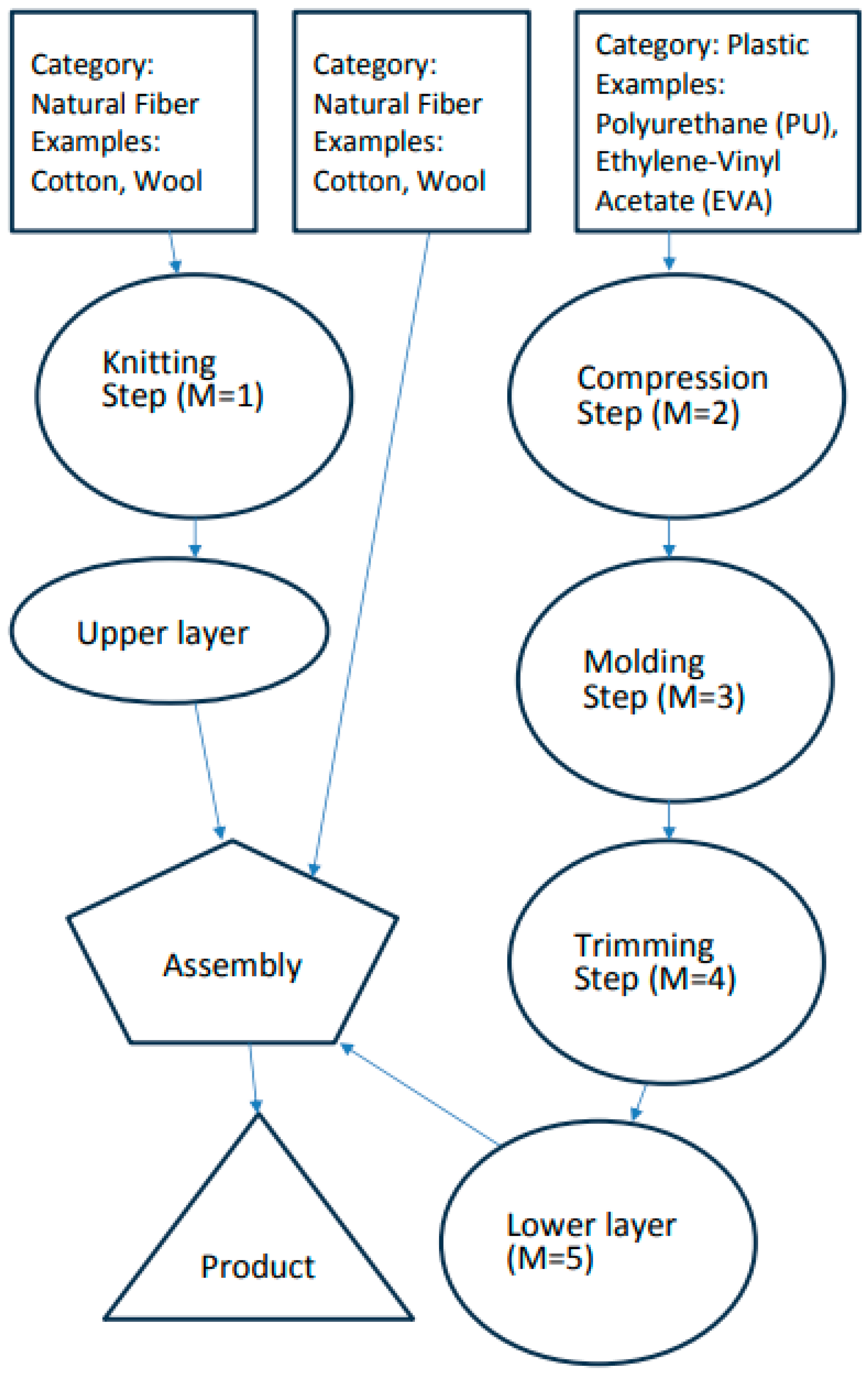
${LH}_{i4}$	In tasks related to pruning, which involve the variable m equaling 4, the quantity of labor hours needed to finish one unit of the i-th product is specified.
${LH}_{i5}$	For tasks that involve combining components, where m is equal to 5, the text outlines the labor hours required to complete one unit of the i-th product.
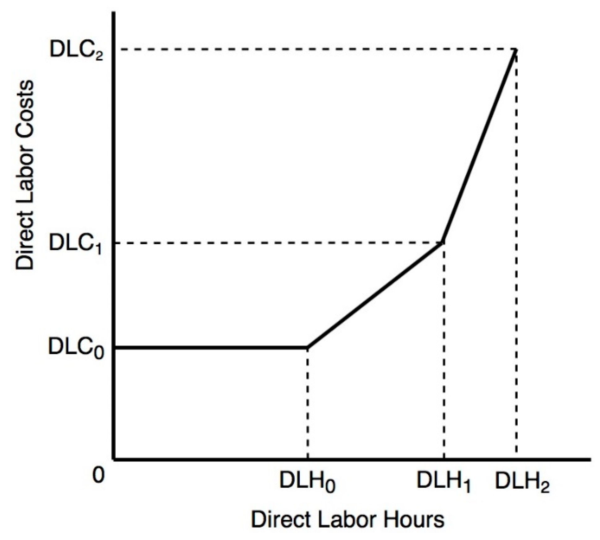
${DLH}_0$	This refers to the aggregate labor hours available for tasks without considering any rush or delayed orders.
${DLH}_1$	This denotes the maximum labor hours allocated during the initial overtime phase, as depicted in Figure 4.
${DLH}_2$	This signifies the greatest amount of labor hours allocated during the second overtime phase, as illustrated in Figure 4.
${DLC}_0$	The total direct labor cost at this point in ${DLC}_0$ = WR0 * ${DLH}_0$.
${DLC}_1$	The total direct labor cost at this point in ${DLC}_1$ = ${DLC}_0$ + WR1 * (${DLH}_1$ − ${DLH}_0$).
${DLC}_2$	The total direct labor cost at this point in ${DLH}_2$= ${DLH}_1$ + WR2 * (${DLH}_2$ − ${DLH}_1$).

If ${\Omega }_1$ is 1, then ${\Omega }_2$ in Equation (33) is 0, ${\eta }_2$ in the Equation (31) is 0, ${\eta }_0, {\eta }_1$ in Equations (29) and (30) fall in [0, 1], and the sum is 1. Therefore, from Equation (28), the company’s total direct labor hours is ${DLH}_0+{\eta }_1\left({DLH}_1-{DLH}_0\right)$, and the company’s total direct labor costs are ${DLC}_0+{\eta }_1\left({DLC}_1-{DLC}_0\right)$, which also means that the company’s total direct labor hours fall in the second section in Figure 4.

3.1.6. Capacity per Machine Hour

This study assumes that knitted shoe production uses three key machines—knitting, pressing, and gluing—to improve efficiency by replacing manual labor, constrained by operation time, space, and labor, with associated costs like depreciation marked as “ℵ”. The constraints concerning machine operation hours are detailed in Equations (36)–(38).

$$\sum _{\mathrm{i}=1}^3{\mathrm{MH}}_{\mathrm{i}1}{\mathrm{X}}_{\mathrm{i}}\le {\mathrm{LMH}}_1$$

(36)

$$\sum _{\mathrm{i}=1}^3{\mathrm{MH}}_{\mathrm{i}2}{\mathrm{X}}_{\mathrm{i}}\le { \mathrm{LMH}}_2$$

(37)

$$\sum _{\mathrm{i}=1}^3{\mathrm{MH}}_{\mathrm{i}5}{\mathrm{X}}_{\mathrm{i}}\le { \mathrm{LMH}}_5$$

(38)

A description of each symbol is provided below:

${MH}_{i1}$	The duration, in machine hours, that the knitting machine takes to produce a single unit of product i.
${MH}_{i2}$	The amount of time, in machine hours, needed by the press to manufacture a single unit of product i.
${MH}_{i5}$	The machine hours necessary for the automatic gluing machine to finish producing a single unit of product i.
${LMH}_1$	The maximum capacity of machine hours that the knitting machine can operate.
${LMH}_2$	The ceiling on the operational machine hours for the press.
${LMH}_5$	The maximum available machine hours for the automatic gluing machine to function.

3.1.7. Batch Level Operation—Formulating a Cost Function for Setup and Material Management

This study explores how carbon emission costs, including government taxes and carbon allowances from trading markets under a cap-and-trade system, affect corporate profitability. It uses four models to examine the implications of carbon tax and trading options on financial outcomes.

The total cost of batch-level operations is calculated as follows:

$$\sum _{\mathrm{i}=1}^3\sum _{m=3,6,7}{C}_m{\lambda }_{\mathrm{i}\mathrm{m}}{\varrho }_{\mathrm{i}\mathrm{m}}$$

The relevant constraints are as follows:

$${\mathrm{X}}_{\mathrm{i}}\le {\mathsf{\beta }}_{\mathrm{i}\mathrm{m}}{\mathsf{\varrho }}_{\mathrm{i}\mathrm{m}}\hspace{1em}\hspace{1em}\hspace{1em}\mathrm{i}=1,2,3;\mathrm{m}=3,6,7$$

(39)

$$\sum _{\mathrm{i}=1}^3{\lambda }_{\mathrm{im}}{\varrho }_{\mathrm{i}\mathrm{m}}\le {\mathrm{R}}_{\mathrm{m}}\hspace{1em}\hspace{1em}\hspace{1em}{\varrho }_{\mathrm{i}\mathrm{j}}\ge 0;\mathrm{m}=3,6,7$$

(40)

A description of each symbol is provided below:

${\varrho }_{im}$	For each type of product, the number of batches processed at each specific batch-level activity is denoted (for product types 1, 2, and 3; during batch processes 3, 6, and 7).
${\beta }_{im}$	The production output for each batch corresponding to each type of product during the specific batch-level stage is detailed (for product types 1, 2, and 3; at batch stages 3, 6, and 7).
${\lambda }_{im}$	Resource use for each batch of product types 1, 2, and 3 is detailed at stages 3, 6, and 7.
$R_m$	The maximum capacity of resources that can be allocated for each batch-level operation is specified (for batch processes 3, 6, and 7).

3.1.8. Product Level Activity—Product Design Cost Function

For a company making three types of knitted shoes, including walking (product 1), jogging (product 2), and high-tops (product 3), each type has specific design costs affecting overall operational costs. Profit calculation requires deducting these design costs from total profit, as shown in constraints 41 and 4.

$$\sum _{\mathrm{i}=1}^3{\mathrm{d}}_8{\mathsf{\Theta }}_{\mathrm{i}8}{\mathsf{\Gamma }}_{\mathrm{i}}$$

The relevant constraints are as follows:

$${\mathrm{X}}_{\mathrm{i}}\le {\mathrm{P}\mathrm{D}}_{\mathrm{i}}{\mathsf{\Gamma }}_{\mathrm{i}}\hspace{1em}\hspace{1em}\hspace{1em}\mathrm{i}=\mathrm{1,2},3$$

(41)

$$\sum _{\mathrm{i}=1}^{\mathrm{n}}{\mathsf{\Theta }}_{\mathrm{i}8}{\mathsf{\Gamma }}_{\mathrm{i}}\le {\mathrm{R}}_8$$

(42)

A description of each symbol is provided below:

${PD}_i$	The existing demand in the market for each type of product.
${\Gamma }_i$	A binary variable, represented as either 0 or 1, used to decide the production status of each product. A Γi value of 1 implies the product is in production, whereas a value of 0 indicates that the product is not being produced.
${\Theta }_{i8}$	The amount of resources expended on the operations at the level of each specific product (for products 1, 2, and 3). The maximum quantity of resources that can be utilized for operations at the product level.
$R_8$	The amount of resources expended on the operations at the level of each specific product (for products 1, 2, and 3). The maximum quantity of resources that can be utilized for operations at the product level.

3.1.9. Direct Raw Material Cost Function

In knitted shoe manufacturing, profit calculations deduct costs for the following key materials: yarn (m = 1), polyurethane (PU) for soles (m = 2), and adhesives (m = 5), as directed by the raw material cost function in Equation (43).

$$\sum _{\mathrm{i}=1}^3\left(\sum _{\mathrm{j}=1}^3{\mathrm{C}\mathrm{M}}_{\mathrm{j}}{\mathrm{R}\mathrm{M}}_{\mathrm{i}\mathrm{j}}\right){\mathrm{X}}_{\mathrm{i}}$$

The relevant constraints are as follows:

$$\sum _{\mathrm{i}=1}^3({\mathrm{R}\mathrm{M}}_{\mathrm{ij}}{\mathrm{X}}_{\mathrm{i}})\le {\mathrm{LMQ}}_{\mathrm{j}}\hspace{1em}\hspace{1em}\hspace{1em}\mathrm{j}=1,2,3$$

(43)

A description of each symbol is provided below:

${CM}_j$	The cost associated with one unit of each type of raw material (categorized as types 1, 2, and 3).
${RM}_{ij}$	The quantity of each type of raw material required to manufacture a single unit of product i (for products 1, 2, and 3, corresponding to raw material types 1, 2, and 3).
${LMQ}_j$	The maximum available quantity for each category of raw material (for raw material types 1, 2, and 3).

3.2. Multi-Period Model

The single-period model analyzes the production and cost parameters within a fixed timeframe. This model helps to understand the immediate impact of various production decisions and carbon tax policies. The multi-period model extends the analysis over multiple time periods, allowing for the assessment of long-term impacts and trends. This model is crucial for evaluating the sustainability of production practices and the effectiveness of carbon management strategies over time.

In the multi-period model, multiple periods (three years) are considered, and factors such as carbon emissions and the pre-borrowing and storage of raw materials are considered.

(1)

Model 1 is an objective function.

This model’s inputs include product market prices, raw material costs, direct labor costs, carbon tax rates, production quantities, carbon emissions, batch operation costs, and machine hours. Specifically, the market price for product 1 is TWD 1705, for product 2 is TWD 1974, and for product 3 is TWD 2178. Raw materials include yarn at TWD 58 per unit, polyurethane at TWD 116 per unit, and glue at TWD 39 per unit. Direct labor costs are TWD 133 per hour for regular labor, TWD 177 per hour for the first overtime, and TWD 221 per hour for the second overtime. Carbon tax rates are TWD 0.9 per kilogram for the first stage, TWD 1.16 per kilogram for the second stage, and TWD 1.417 per kilogram for the third stage. Production quantities are 34,818 pairs for product 1, 14,454 pairs for product 2, and 29,582 pairs for product 3. The output data include a total revenue of TWD 152.3 million, product revenues of TWD 59.4 million for product 1, TWD 28.5 million for product 2, and TWD 64.4 million for product 3. The total profit is TWD 45.6 million. Direct labor costs amount to TWD 16.0 million for 120,000 regular hours, and batch costs are TWD 16.4 million, including TWD 1.2 million for molding, TWD 3.2 million for setup, and TWD 1.2 million for handling. The carbon tax cost is TWD 251,000 for a total emission of 250,000 kg.

$$\begin{array}{l}\pi ={\displaystyle \sum _{\mathrm{t}=1}^{\mathrm{T}}}{\displaystyle \sum _{\mathrm{i}=1}^3}{\mathrm{P}}_{\mathrm{i}}{\mathrm{X}}_{\mathrm{i}\mathrm{t}}-{\displaystyle \sum _{\mathrm{t}}^{\mathrm{T}}}({\displaystyle \sum _{\mathrm{i}=1}^3}{\displaystyle \sum _{\mathrm{j}=1}^3}{\mathrm{C}\mathrm{M}}_{\mathrm{j}}{\mathrm{R}\mathrm{M}}_{\mathrm{i}\mathrm{j}}{)\mathrm{X}}_{\mathrm{i}\mathrm{t}}-{\displaystyle \sum _{\mathrm{t}}^{\mathrm{T}}}{\mathrm{D}\mathrm{L}\mathrm{C}}_0+{\mathsf{\eta }}_{1\mathrm{t}}\left({\mathrm{D}\mathrm{L}\mathrm{C}}_1-{\mathrm{D}\mathrm{L}\mathrm{C}}_0\right)+{\mathsf{\eta }}_{2\mathrm{t}}\left({\mathrm{D}\mathrm{L}\mathrm{C}}_2-{\mathrm{D}\mathrm{L}\mathrm{C}}_0\right)\\ \hspace{1em}\hspace{1em}\hspace{1em}\hspace{1em}\hspace{1em}\hspace{1em}-{\displaystyle \sum _{\mathrm{t}}^{\mathrm{T}}}({\displaystyle \sum _{\mathrm{i}=1}^3}{\displaystyle \sum _{m=3,6,7}}{C}_m{\lambda }_{\mathrm{i}\mathrm{m}}{\varrho }_{\mathrm{i}\mathrm{m}\mathrm{t}})-{\displaystyle \sum _{\mathrm{t}=1}^{\mathrm{T}}}{\displaystyle \sum _{\mathrm{i}=1}^3}{\mathrm{d}}_8{\mathsf{\Theta }}_{\mathrm{i}8}{\mathsf{\Gamma }}_{\mathrm{i}\mathrm{t}}-{\displaystyle \sum _{\mathrm{t}=1}^{\mathrm{T}}}({\mathrm{C}\mathrm{T}}_1{\omega }_{1\mathrm{t}}+{\mathrm{C}\mathrm{T}}_2{\omega }_{2\mathrm{t}}+{\mathrm{C}\mathrm{T}}_3{\omega }_{3\mathrm{t}})-{\displaystyle \sum _{\mathrm{t}=1}^{\mathrm{T}}}{\mathrm{F}}_{\mathrm{t}}\end{array}$$

(44)

(2)

Model 2 evaluates a carbon tax system with increasing rates and carbon credit trading.

This model has the same inputs as Model 1 but includes carbon trading mechanisms. The output data show a total revenue of TWD 160.2 million, with product revenues of TWD 45.5 million for product 1, TWD 49.4 million for product 2, and TWD 65.3 million for product 3. The total profit increases to TWD 49.8 million. Direct labor costs rise to TWD 18.0 million because of the inclusion of 11,700 overtime hours on top of the regular 120,000 h. The batch costs are TWD 16.6 million, with TWD 1.2 million for molding, TWD 3.3 million for setup, and TWD 1.2 million for handling. The carbon tax in this model is TWD 277,000 for 272,000 kg of emissions, divided into 47,000 kg for product 1, 82,000 kg for product 2, and 143,000 kg for product 3, plus an additional TWD 16,000 for carbon rights.

$$\begin{array}{l}\pi ={\displaystyle \sum _{\mathrm{t}=1}^{\mathrm{T}}}{\displaystyle \sum _{\mathrm{i}=1}^3}{\mathrm{P}}_{\mathrm{i}}{\mathrm{X}}_{\mathrm{i}\mathrm{t}}-{\displaystyle \sum _{\mathrm{t}=1}^{\mathrm{T}}}({\displaystyle \sum _{\mathrm{i}=1}^3}{\displaystyle \sum _{\mathrm{j}=1}^3}{\mathrm{C}\mathrm{M}}_{\mathrm{j}}{\mathrm{R}\mathrm{M}}_{\mathrm{i}\mathrm{j}}{)\mathrm{X}}_{\mathrm{i}\mathrm{t}}-{\displaystyle \sum _{\mathrm{t}=1}^{\mathrm{T}}}{\mathrm{D}\mathrm{L}\mathrm{C}}_0+{\mathsf{\eta }}_{1\mathrm{t}}\left({\mathrm{D}\mathrm{L}\mathrm{C}}_1-{\mathrm{D}\mathrm{L}\mathrm{C}}_0\right)+{\mathsf{\eta }}_{2\mathrm{t}}\left({\mathrm{D}\mathrm{L}\mathrm{C}}_2-{\mathrm{D}\mathrm{L}\mathrm{C}}_0\right)\\ \hspace{1em}\hspace{1em}\hspace{1em}\hspace{1em}\hspace{1em}\hspace{1em}-{\displaystyle \sum _{\mathrm{t}=1}^{\mathrm{T}}}({\displaystyle \sum _{\mathrm{i}=1}^3}{\displaystyle \sum _{m=3,6,7}}{C}_m{\lambda }_{\mathrm{i}\mathrm{m}}{\varrho }_{\mathrm{i}\mathrm{m}\mathrm{t}})-{\displaystyle \sum _{\mathrm{t}=1}^{\mathrm{T}}}{\displaystyle \sum _{\mathrm{i}=1}^3}{\mathrm{d}}_8{\mathsf{\Theta }}_{\mathrm{i}8}{\mathsf{\Gamma }}_{\mathrm{i}\mathrm{t}}\\ \hspace{1em}\hspace{1em}\hspace{1em}\hspace{1em}\hspace{1em}\hspace{1em}-[{\displaystyle \sum _{\mathrm{t}=1}^{\mathrm{T}}}\left({\mathrm{C}\mathrm{T}}_1{\omega }_{1\mathrm{t}}+{\mathrm{C}\mathrm{T}}_2{\omega }_{2\mathrm{t}}+{\mathrm{C}\mathrm{T}}_3{\omega }_{3\mathrm{t}}\right)-\alpha (\mathrm{M}\mathrm{C}\mathrm{E}\mathrm{Q}\\ \hspace{1em}\hspace{1em}\hspace{1em}\hspace{1em}\hspace{1em}\hspace{1em}-{\displaystyle \sum _{\mathrm{t}=1}^{\mathrm{T}}}{q}_t)]{\sigma }_1-[{\displaystyle \sum _{\mathrm{t}=1}^{\mathrm{T}}}\left({\mathrm{C}\mathrm{T}}_1{\omega }_{1\mathrm{t}}+{\mathrm{C}\mathrm{T}}_2{\omega }_{2\mathrm{t}}+{\mathrm{C}\mathrm{T}}_3{\omega }_{3\mathrm{t}}\right)+\alpha ({\displaystyle \sum _{\mathrm{t}=1}^{\mathrm{T}}}{q}_t-\mathrm{M}\mathrm{C}\mathrm{E}\mathrm{Q})]{\sigma }_2-{\displaystyle \sum _{\mathrm{t}=1}^{\mathrm{T}}}{\mathrm{F}}_{\mathrm{t}}\end{array}$$

(45)

(3)

Model 3 is a carbon tax pricing model with a tiered, incrementally increasing tax rate without the option for trading carbon emission allowances.

This model uses a stepped progressive carbon tax rate without carbon trading. The input data are the same as Model 1. The output data show a total revenue of TWD 152.3 million, with the same breakdown across the three products. Production volumes are 34,800 pairs for product 114,500 pairs for product 2, and 29,600 pairs for product 3. The total profit remains consistent with Model 1 at TWD 45.6 million. Direct labor costs are TWD 16.0 million, and batch costs remain at TWD 16.4 million. The carbon tax increases to TWD 290,000 for the same total emissions of 250,000 kg, now distributed as 62,000 kg for product 147,000 kg for product 2, and 141,000 kg for product 3.

$$\begin{array}{l}\pi ={\displaystyle \sum _{\mathrm{t}=1}^{\mathrm{T}}}{\displaystyle \sum _{\mathrm{i}=1}^3}{\mathrm{P}}_{\mathrm{i}}{\mathrm{X}}_{\mathrm{i}\mathrm{t}}-{\displaystyle \sum _{\mathrm{t}=1}^{\mathrm{T}}}({\displaystyle \sum _{\mathrm{i}=1}^3}{\displaystyle \sum _{\mathrm{j}=1}^3}{\mathrm{C}\mathrm{M}}_{\mathrm{j}}{\mathrm{R}\mathrm{M}}_{\mathrm{i}\mathrm{j}}{)\mathrm{X}}_{\mathrm{i}\mathrm{t}}-{\displaystyle \sum _{\mathrm{t}=1}^{\mathrm{T}}}{\mathrm{D}\mathrm{L}\mathrm{C}}_0+{\mathsf{\eta }}_{1\mathrm{t}}\left({\mathrm{D}\mathrm{L}\mathrm{C}}_1-{\mathrm{D}\mathrm{L}\mathrm{C}}_0\right)+{\mathsf{\eta }}_{2\mathrm{t}}\left({\mathrm{D}\mathrm{L}\mathrm{C}}_2-{\mathrm{D}\mathrm{L}\mathrm{C}}_0\right)\\ \hspace{1em}\hspace{1em}\hspace{1em}\hspace{1em}\hspace{1em}\hspace{1em}-{\displaystyle \sum _{\mathrm{t}=1}^{\mathrm{T}}}\left({\displaystyle \sum _{\mathrm{i}=1}^3}{\displaystyle \sum _{m=3,6,7}}{C}_m{\lambda }_{\mathrm{i}\mathrm{m}}{\varrho }_{\mathrm{i}\mathrm{m}\mathrm{t}}\right)-{\displaystyle \sum _{\mathrm{t}=1}^{\mathrm{T}}}{\displaystyle \sum _{\mathrm{i}=1}^3}{\mathrm{d}}_8{\mathsf{\Theta }}_{\mathrm{i}8}{\mathsf{\Gamma }}_{\mathrm{i}\mathrm{t}}-{\displaystyle \sum _{\mathrm{t}=1}^{\mathrm{T}}}{\displaystyle \sum _{\mathrm{i}=1}^3}{\mathrm{d}}_8{\mathsf{\Theta }}_{\mathrm{i}8}{\mathsf{\Gamma }}_{\mathrm{i}\mathrm{t}}\\ \hspace{1em}\hspace{1em}\hspace{1em}\hspace{1em}\hspace{1em}\hspace{1em}-{\displaystyle \sum _{\mathrm{t}=1}^{\mathrm{T}}}({\mathrm{T}\mathrm{R}}_1{\mathrm{Q}}_{1\mathrm{t}}+{\mathrm{T}\mathrm{R}}_2{\mathrm{Q}}_{2\mathrm{t}}+{\mathrm{T}\mathrm{R}}_3{\mathrm{Q}}_{3\mathrm{t}})-{\displaystyle \sum _{\mathrm{t}=1}^{\mathrm{T}}}{\mathrm{F}}_{\mathrm{t}}\end{array}$$

(46)

(4)

Model 4 is a carbon tax framework using a segmented, progressively increasing rate, integrating the ability to trade carbon emission permits.

This model combines a stepped progressive tax rate with carbon rights trading. The input data are the same as in the previous models. The output data show a total revenue of TWD 160.2 million, with product-specific revenues of TWD 45.5 million for product 1, TWD 49.4 million for product 2, and TWD 65.3 million for product 3. The production quantities are 26,700 pairs for product 1, 25,000 pairs for product 2, and 30,000 pairs for product 3. The total profit in this scenario is the highest at TWD 49.8 million. The direct labor costs are TWD 18.0 million, including overtime hours. The batch costs are TWD 16.6 million, similar to Model 2. The carbon tax is TWD 316,000 for 272,000 kg of emissions, divided into 47,000 kg for product 1, 82,000 kg for product 2, and 143,000 kg for product 3, along with an additional TWD 16,000 for carbon rights.

$$\begin{array}{l}\pi ={\displaystyle \sum _{\mathrm{t}=1}^{\mathrm{T}}}{\displaystyle \sum _{\mathrm{i}=1}^3}{\mathrm{P}}_{\mathrm{i}}{\mathrm{X}}_{\mathrm{i}\mathrm{t}}-{\displaystyle \sum _{\mathrm{t}=1}^{\mathrm{T}}}({\displaystyle \sum _{\mathrm{i}=1}^3}{\displaystyle \sum _{\mathrm{j}=1}^3}{\mathrm{C}\mathrm{M}}_{\mathrm{j}}{\mathrm{R}\mathrm{M}}_{\mathrm{i}\mathrm{j}}{)\mathrm{X}}_{\mathrm{i}\mathrm{t}}-{\displaystyle \sum _{\mathrm{t}=1}^{\mathrm{T}}}{\mathrm{D}\mathrm{L}\mathrm{C}}_0+{\mathsf{\eta }}_{1\mathrm{t}}\left({\mathrm{D}\mathrm{L}\mathrm{C}}_1-{\mathrm{D}\mathrm{L}\mathrm{C}}_0\right)+{\mathsf{\eta }}_{2\mathrm{t}}\left({\mathrm{D}\mathrm{L}\mathrm{C}}_2-{\mathrm{D}\mathrm{L}\mathrm{C}}_0\right)\\ \hspace{1em}\hspace{1em}\hspace{1em}\hspace{1em}\hspace{1em}\hspace{1em}-{\displaystyle \sum _{\mathrm{t}=1}^{\mathrm{T}}}\left({\displaystyle \sum _{\mathrm{i}=1}^3}{\displaystyle \sum _{m=3,6,7}}{C}_m{\lambda }_{\mathrm{i}\mathrm{m}}{\varrho }_{\mathrm{i}\mathrm{m}\mathrm{t}}\right)-{\displaystyle \sum _{\mathrm{t}=1}^{\mathrm{T}}}{\displaystyle \sum _{\mathrm{i}=1}^3}{\mathrm{d}}_8{\mathsf{\Theta }}_{\mathrm{i}8}{\mathsf{\Gamma }}_{\mathrm{i}\mathrm{t}}\\ \hspace{1em}\hspace{1em}\hspace{1em}\hspace{1em}\hspace{1em}\hspace{1em}-[{\displaystyle \sum _{\mathrm{t}=1}^{\mathrm{T}}}\left({\mathrm{T}\mathrm{R}}_1{\mathrm{Q}}_{1\mathrm{t}}+{\mathrm{T}\mathrm{R}}_2{\mathrm{Q}}_{2\mathrm{t}}+{\mathrm{T}\mathrm{R}}_3{\mathrm{Q}}_{3\mathrm{t}}\right)-\alpha (\mathrm{M}\mathrm{C}\mathrm{E}\mathrm{Q}\\ \hspace{1em}\hspace{1em}\hspace{1em}\hspace{1em}\hspace{1em}\hspace{1em}-{\displaystyle \sum _{\mathrm{t}=1}^{\mathrm{T}}}{q}_t)]{\sigma }_1-[{\displaystyle \sum _{\mathrm{t}=1}^{\mathrm{T}}}\left({\mathrm{T}\mathrm{R}}_1{\mathrm{Q}}_{1\mathrm{t}}+{\mathrm{T}\mathrm{R}}_2{\mathrm{Q}}_{2\mathrm{t}}+{\mathrm{T}\mathrm{R}}_3{\mathrm{Q}}_{3\mathrm{t}}\right)+\alpha ({\displaystyle \sum _{\mathrm{t}=1}^{\mathrm{T}}}{q}_t-\mathrm{M}\mathrm{C}\mathrm{E}\mathrm{Q})]{\sigma }_2-{\displaystyle \sum _{\mathrm{t}=1}^{\mathrm{T}}}{\mathrm{F}}_{\mathrm{t}}\end{array}$$

(47)

4. Research Results and Analysis

4.1. Assumptions of Single-Period and Multi-Period Model Parameter Data

This study presents four scenarios for knitted shoe manufacturers, considering various costs at the individual activity, batch process, product, and carbon emission levels, as well as fixed expenses. In order to provide a complete example, some of the data are based on assumptions according to the understanding of the footwear industry, while some are provided by the case company.

Table 1. Illustrative data.

					Maximum Available Resources	Product 1 (i = 3)	Product 2 (i = 2)	Product 3 (i = 1)
Market price of product			m	Pi		TWD 2178	TWD 1974	TWD 1705
Fundamental resources (unit level)	j equal to 1 (string)	M1 = TWD 58/unit		RMi1	LMQ1 = $\mathrm{265,938}$	$2$	$1.5$	$1$
	j equal to 2 (PU)	M2 = TWD 116/unit		RMi2	LMQ2 = 364,000	$2$	$2$	$2$
	j equal to 3 (glue)	M3 = TWD 39/unit		RMi3	LMQ3 = 156,000	$1.2$	$1$	$0.5$
Unit level job
labor hours	m equal to 4 (trimming)		4	RLHi4		$0.4$	$0.3$	$0.2$
	m equal to 5 (combination)		5	RLHi5		$1.6$	$1.5$	$0.8$
machine hour	m equal to 1 (knitting)		1	RMHi1	LMH1 = 401,500	8	4	1
	m equal to 2 (pressing)		2	RMHi2	LMH2 = 24,024	0.2	0.14	0.1
	m equal to 5 (combination)		5	RMHi5	LMH5 = 64,064	0.5	0.4	0.2
Batch level	job element
forming	forming hours	C3 = TWD 100/h	3	$\mathsf{\beta }$i3	R3 = 120,900	2	2	2
				$\mathsf{\lambda }$i3		2	3	4
setting	setting hours	C6 = TWD 40/h	6	$\mathsf{\beta }$i6	R6 = 713,284	2	3	6
				$\mathsf{\lambda }$i6		2	3	6
material handling	handling hours	C7 = TWD 15/h	7	$\mathsf{\beta }$i7	R7 = 436,800	2	4	6
				$\mathsf{\lambda }$i7		3	4	6
Product level	product design	d8 = TWD 150/h	8	$\mathsf{\Theta }$i8	C8 = 10,000	5000	1500	3000
Labor cost cap on costs for direct labor	DLC0 = TWD 15,960,000	DLC1 = TWD 22,910,790	DLC2 = TWD 31,589,640
allocated hours for direct labor	DLH0 = 120,000	DLH1 = 39,270	DLH2 = 78,540
hourly wage rate	WR0 = TWD 133/h	WR1 = TWD 177/h	WR2 = TWD 221/h
Carbon emissions
carbon emissions during production	m = 1 (knitting)			CEi1	MCEQ = 250,000 kg	1.43	0.98	0.53
	m = 2 (pressing)			CEi2	SMCEQ = 677,500 kg	0.95	0.65	0.35
	m = (combination)			CEi5		2.39	1.64	0.89
Carbon tax cost	CT1 = TWD 135,000	CT2 = TWD 425,000	T3 = TWD 313,667,020
Carbon emission caps for each level	CEQ1 = 150,000 kg	CEQ2 = 400,000 kg	CEQ3 = 221,460,000 kg
Carbon tax rates for each level	TR1 = TWD 0.9/kg	TR2 = TWD 1.16/kg	TR3 = TWD 1.417/kg
Carbon rights cost	LPCRC = TWD 36,500	LPCEQ = 50,000 kg	$\alpha$ = TWD 0.73/kg		MPCEQ = 300,000 kg
	SLPCRC = TWD 98,910	LPCEQ = 135,500 kg			SMPCEQ = 813,000 kg

provides an overview of the various data types used in this paper. It includes product market price, RM1, RM2, RM3, labor hours, and carbon emissions. The product column identifies the type of footwear being analyzed, which includes product 1, product 2, and product 3. The market price column indicates the selling price per unit in New Taiwan Dollars (TWD). The columns RM1, RM2, and RM3 specify the raw material requirements per unit, including the amount of string, PU, and glue needed for each product. Labor hours denote the required labor hours per unit for various production stages. Lastly, the carbon emissions column measures the carbon emissions generated per unit during the production process.

Retail prices for products 1, 2, and 3 are TWD 1,705, TWD 1,974, and TWD 2,178, respectively. Direct labor compensation rates across three tiers are TWD 133, TWD 177, and TWD 221 per hour. Carbon emission tax rates for three levels are TWD 0.9, TWD 1.16, and TWD 1.417 per kilogram. Table 1,

Table 2. Single-period continuous carbon tax model 1.

π

= (1705 * X1 + 1974 * X2 + 2178 * X3) − [(58 + 232 + 20)X1 + (87 + 232 + 39)X2 + (116 + 232 + 47)X3] − (15,960,000 + 6,950,790$\mathsf{\eta }$1 + 15,629,640$\mathsf{\eta }$2) − [(4 * 100)$\ast {\varrho }_{13}$ + (3 * 100)${ \ast \varrho }_{23}$ + (2 * 100)$\ast {\varrho }_{33}$] − [(6 * 40)${\varrho }_{16}$ + (3 * 40)${\varrho }_{26}$ + (2 * 40)${\varrho }_{36}$] + [(6 * 15)${\varrho }_{17}$ + (4 * 15)${\varrho }_{27}$ + (3 * 15)${\varrho }_{37}$)] − (450,000${\mathsf{\Gamma }}_1$ + 225,000${\mathsf{\Gamma }}_2$ + 750,000$\ast {\mathsf{\Gamma }}_3$) − (135,000$\ast {\omega }_1$ + 425,000${ \ast \omega }_2$ + 313,667,020$\ast {\omega }_3$) − 44,996,392;

carbon tax constraints: (1.77 * X1 + 3.27 * X2 + 4.77 * X3) = 150,000${ \ast \omega }_1$ + 400,000$\ast {\omega }_2$ + 221,460,000$\ast {\omega }_3$; (1.77 * X1 + 3.27 * X2 + 4.77 * X3) ≤ 250,000; ${\omega }_0$ − ${\epsilon }_1$ ≤ 0; ${\omega }_1$ − ${\epsilon }_1$ − ${\epsilon }_2$ ≤ 0; ${\omega }_2$ − ${\epsilon }_2$ − ${\epsilon }_3$ ≤ 0; ${\omega }_3$ − ${\epsilon }_3$ ≤ 0; ${\omega }_0$ + ${\omega }_1$ + ${\omega }_2$ + ${\omega }_3$ = 1; ${\epsilon }_1$ + ${\epsilon }_2$ + ${\epsilon }_3$ = 1

,

Table 3. Single-period continuous carbon tax with carbon trading model 2.

π	= (1705X1 + 1974X2 + 2178X3) − [(58 + 232 + 20)X1 + (87 + 232 + 39)X2 + (116 + 232 + 47)X3] − (15,960,000 + 6,950,790$\mathsf{\eta }$1 + 15,629,640$\mathsf{\eta }$2) − [(4 * 100)${\varrho }_{13}$ + (3 * 100)${\varrho }_{23}$ + (2 * 100)${\varrho }_{33}$] − [(6 * 40)${\varrho }_{16}$ + (3 * 40)${\varrho }_{26}$ + (2 * 40)${\varrho }_{36}$] + [(6 * 15)${\varrho }_{17}$ + (4 * 15)${\varrho }_{27}$ + (3 * 15)${\varrho }_{37}$)] − (450,000${\mathsf{\Gamma }}_1$ + 225,000${\mathsf{\Gamma }}_2$ + 750,000${\mathsf{\Gamma }}_3$) − ((135,000$\ast {\omega }_1$ + 425,000$\ast {\omega }_2$ + 313,667,020$\ast {\omega }_3$) − (250,000 − (${\mathsf{\Lambda }}_1+{\mathsf{\Lambda }}_2$)) * 0.73)${\sigma }_1$ − ((135,000$\ast {\omega }_1$ + 425,000$\ast {\omega }_2$ + 313,667,020$\ast {\omega }_3$) + ((${\mathsf{\Lambda }}_1+{\mathsf{\Lambda }}_2$) − 250,000) * 0.73)${\sigma }_2$ − 44,996,392;
carbon tax constraints: (1.77 * X1 + 3.27 * X2 + 4.77 * X3) = 150,000$\ast {\omega }_1$ + 400,000$\ast {\omega }_2$ + 221,460,000${\omega }_3$; ${\omega }_0$ − ${\epsilon }_1$ ≤ 0; ${\omega }_1$ − ${\epsilon }_1$ − ${\epsilon }_2$ ≤ 0; ${\omega }_2$ − ${\epsilon }_2$ − ${\epsilon }_3$ ≤ 0; ${\omega }_3$ − ${\epsilon }_3$ ≤ 0; ${\omega }_0$ + ${\omega }_1$ + ${\omega }_2$ + ${\omega }_3$ = 1; ${\epsilon }_1$ + ${\epsilon }_2$ + ${\epsilon }_3$ = 1
carbon right constraint: (1.77 * X1 + 3.27 * X2 + 4.77 * X3) = ${\mathsf{\Lambda }}_1+{\mathsf{\Lambda }}_2$; ${\mathsf{\Lambda }}_1$ ≤ ${\sigma }_1 \ast$250,000; ${\sigma }_2 \ast \mathrm{250,000}<{\mathsf{\Lambda }}_2$; ${\mathsf{\Lambda }}_2$ ≤ ${\sigma }_2 \ast$300,000; ${\sigma }_1$ + ${\sigma }_2=$ 1

,

Table 4. Single-period discontinuous carbon tax Model 3.

π

= (1705 * X1 + 1974 * X2 + 2178 * X3) − [(58 + 232 + 20)X1 + (87 + 232 + 39)X2 + (116 + 232 + 47)X3] − (15,960,000 + 6,950,790$\mathsf{\eta }$1 + 15,629,640$\mathsf{\eta }$2) − [(4 * 100)${\varrho }_{13}$ + (3 * 100)${\varrho }_{23}$ + (2 * 100)${\varrho }_{33}$] − [(6 * 40)${\varrho }_{16}$ + (3 * 40)${\varrho }_{26}$ + (2 * 40)${\varrho }_{36}$] + [(6 * 15)${\varrho }_{17}$ + (4 * 15)${\varrho }_{27}$ + (3 * 15)${\varrho }_{37}$)] − (450,000${\mathsf{\Gamma }}_1$ + 225,000${\mathsf{\Gamma }}_2$ + 750,000${\mathsf{\Gamma }}_3$) − ($0.9{\mathrm{Q}}_1+1.16{\mathrm{Q}}_2+1.417{\mathrm{Q}}_3$) − 44,996,392;

carbon tax constraints: (1.77 * X1 + 3.27 * X2 + 4.77 * X3) = Q1 + Q2 + Q3; (1.77 * X1 + 3.27 * X2 + 4.77 * X3) ≤ 250,000; $0\le {\mathrm{Q}}_1$; ${\mathrm{Q}}_1\le {\mathrm{\varnothing }}_1 \ast \mathrm{150,000}$; ${\mathrm{\varnothing }}_2 \ast \mathrm{150,000}<{\mathrm{Q}}_2$; ${\mathrm{Q}}_2$ ≤ ${\mathrm{\varnothing }}_2 \ast$400,000; ${\mathrm{Q}}_3>{\mathrm{\varnothing }}_3 \ast \mathrm{400,000}$; ${\mathrm{Q}}_3\le {\mathrm{\varnothing }}_3 \ast \mathrm{999,999}$; ${\mathrm{\varnothing }}_1+{\mathrm{\varnothing }}_2+{\mathrm{\varnothing }}_3=1$

,

Table 5. Demonstration data added to single-period Model 4.

π	= (1705 * X1 + 1974 * X2 + 2178 * X3) − [(58 + 232 + 20)X1 + (87 + 232 + 39)X2 + (116 + 232 + 47)X3] − (15,960,000 + 6,950,790$\ast \mathsf{\eta }$1 + 15,629,640$\ast \mathsf{\eta }$2) − [(4 * 100)${\varrho }_{13}$ + (3 * 100)${\varrho }_{23}$ + (2 * 100)${\varrho }_{33}$] − [(6 * 40)${\varrho }_{16}$ + (3 * 40)${\varrho }_{26}$ + (2 * 40)${\varrho }_{36}$] + [(6 * 15)${\varrho }_{17}$ + (4 * 15)${\varrho }_{27}$ + (3 * 15)${\varrho }_{37}$)] − (450,000${\mathsf{\Gamma }}_1$ + 225,000${\mathsf{\Gamma }}_2$ + 750,000${\mathsf{\Gamma }}_3$) − (($0.9{\mathrm{Q}}_1+1.16{\mathrm{Q}}_2+1.417{\mathrm{Q}}_3$) − (250,000 − (${\mathsf{\Lambda }}_1+{\mathsf{\Lambda }}_2$)) * 0.73)${\sigma }_1$ − (($0.9 \ast {\mathrm{Q}}_1+1.16 \ast {\mathrm{Q}}_2+1.417{ \ast \mathrm{Q}}_3$) + ((${\mathsf{\Lambda }}_1+{\mathsf{\Lambda }}_2$) − 250,000) * 0.73)${\sigma }_2$ − 44,996,392;
carbon tax constraints: (1.77 * X1 + 3.27 * X2 + 4.77 * X3) = Q1 + Q2 + Q3; $0\le {\mathrm{Q}}_1$; ${\mathrm{Q}}_1\le {\mathrm{\varnothing }}_1\mathrm{150,000}$; ${\mathrm{\varnothing }}_2\mathrm{150,000}<{\mathrm{Q}}_2$; ${\mathrm{Q}}_2$ ≤ ${\mathrm{\varnothing }}_2 \ast$400,000; ${\mathrm{Q}}_3>{\mathrm{\varnothing }}_3 \ast \mathrm{400,000}$; ${\mathrm{Q}}_3\le {\mathrm{\varnothing }}_3 \ast \mathrm{999,999}$; ${\mathrm{\varnothing }}_1+{\mathrm{\varnothing }}_2+{\mathrm{\varnothing }}_3=1$
carbon right constraint: (1.77 * X1 + 3.27 * X2 + 4.77 * X3) = ${\mathsf{\Lambda }}_1+{\mathsf{\Lambda }}_2$; ${\mathsf{\Lambda }}_1$ ≤ ${\sigma }_1 \ast$250,000; ${\sigma }_2 \ast \mathrm{250,000}<{\mathsf{\Lambda }}_2$; ${\mathsf{\Lambda }}_2$ ≤${\sigma }_2$ * 300,000; ${\sigma }_1$ + ${\sigma }_2=$ 1;

and

Table 6. Common restrictions for single-period models.

The target equation is constrained by the following: Direct raw material restrictions 1 * X1 + 1.5 * X2 + 2 * X3 ≤ 265,938; 2 * X1 + 2 * X2 + 2 * X3 ≤ 364,000; 0.5 * X1 + 1 * X2 + 1.2 * X3 ≤ 156,000;

Direct manual restriction (1 * X1 + 1.8 * X2 + 2 * X3) ≤ (120,000 +${\mathsf{\eta }}_1 \ast$39,270 + ${\mathsf{\eta }}_2$* 78,540); ${\mathsf{\eta }}_0-{\mathsf{\Omega }}_1\le 0$; ${\mathsf{\eta }}_1-{\mathsf{\Omega }}_1-{\mathsf{\Omega }}_2\le 0;(\mathrm{b}\mathrm{r}\mathrm{e}\mathrm{a}\mathrm{k}){\mathsf{\eta }}_2-{\mathsf{\Omega }}_2\le 0$; ${\mathsf{\eta }}_0+{\mathsf{\eta }}_1+{\mathsf{\eta }}_2=1$; ${\mathsf{\Omega }}_1+{\mathsf{\Omega }}_2=1$;

Machine hour limit 1 * X1 + 4 * X2 + 8 * X3 ≤ 401,500; 0.1 * X1 + 0.14 * X2 + 0.2 * X3 ≤ 24,024; 0.2 * X1 + 0.4 * X2 + 0.5 * X3 ≤ 64,064;

Batch-level job limits (forming) X1 − 2 * ${\varrho }_{13}$ ≤ 0; X2 − 2 * ${\varrho }_{23}$ ≤ 0; X3 − 2$\ast {\varrho }_{33}$ ≤ 0; 4$\ast {\varrho }_{13}$ + 3$\ast {\varrho }_{23}$ + 2$\ast {\varrho }_{33}$ ≤ 120,900;

Batch-level job limits (settings) X1 − 6$\ast {\varrho }_{16}$ ≤ 0; X2 − 3$\ast {\varrho }_{26}$ ≤ 0; X3 − 2$\ast {\varrho }_{36}$ ≤ 0; 6${\varrho }_{16}$ + 3$\ast {\varrho }_{26}$ + 2$\ast {\varrho }_{36}$ ≤ 713,284;

Batch-level job limits (material handling) X1 − 6$\ast {\varrho }_{17}$ ≤ 0; X2 − 4$\ast {\varrho }_{27}$ ≤ 0; X3 − 3$\ast {\varrho }_{37}$ ≤ 0; 6${\varrho }_{17}$ + 4$\ast {\varrho }_{27}$ + 3${\varrho }_{37}$ ≤ 436,800;

Product-level assignments (product design) X1 − 100,000$\ast {\mathsf{\Gamma }}_1$ ≤ 0; X2 − 25,000$\ast {\mathsf{\Gamma }}_2$ ≤ 0; X3 − 30,000$\ast {\mathsf{\Gamma }}_3$ ≤ 0; 3000$\ast {\mathsf{\Gamma }}_1$ + 1500$\ast {\mathsf{\Gamma }}_2$ + 5000$\ast {\mathsf{\Gamma }}_3$ ≤ 10,000;

present the foundational parameters and their application in the formulas for each scenario, while

Table 7. Comparison of single-period models.

	Profit	The Output of Each Product	Carbon Emission	Carbon Tax Cost	The Cost of Carbon Rights	Labor Hours	Forming (Forming Hours)	Setting (Setting Hours)	Material Handling (Handling Hours)
Model 1 Continuous carbon tax	TWD 45,614,175	X1: 34,818 X2: 14,454 X3: 29,582	249,999	TWD 250,998	0	119,999	120,899	78,854	78,857
Model 2 Continuous carbon tax with carbon trading	49,807,842	X1: 26,700 X2: 25,000 X3: 30,000	272,109	276,646	16,140	131,700	120,900	81,702	81,700
Model 3 Discontinuous carbon tax	45,575,175	X1: 34,818 X2: 14,454 X3: 29,582	249,999	289,998	0	119,999	120,899	78,854	78,857
Model 4 Discontinuous carbon tax with carbon trading	49,768,842	X1: 26,700 X2: 25,000 X3: 30,000	272,109	315,646	16,140	131,700	120,900	81,702	81,700

compiles the common constraint equations for the single-period model.

• Model 1: Continuous and progressive carbon tax cost function without carbon emission trading. The carbon tax cost increases continuously with emissions.
• Model 2: Single-period model with a continuous carbon tax rate based on emission levels and the option for carbon trading.
• Model 3: Single-period model with a stepwise carbon tax rate structure. The tax rate remains constant within each emission range but increases abruptly when emissions exceed predetermined threshold.
• Model 4: Combines a stepped progressive tax rate with carbon rights trading.

4.2. Model Analysis

This study presents a model that merges activity-based costing, the theory of constraints, and carbon emission costs to enhance profit margins under resource constraints. Using LINGO 21 software and the initial parameters in Table 1, it analyzes variables like total profit, production volumes, direct labor, batch-level costs, product-level expenses, and carbon emission costs. The results, shown in Table 7 (for the single-period models) and

Table 8. Comparison of multi-period models.

	Profit	The Output of Each Product	Carbon Emission	Carbon Tax Cost	Pre-Borrow or Store Carbon Emissions	Expense Related to Carbon Credits	Labor Hours	Forming (Forming Hours)	(Adjustment Duration) Management of Materials	(Management Duration)
Model 1 Continuous carbon tax	TWD 118,037,916	X11: 30,600 X21: 25,000 X31: 22,198	241,797	TWD 241,483	(8204)	0	119,996	120,898	77,800	77,800
		X12: 36,768 X22: 24,996 X32: 9870	193,896	185,920	(31,104)		114,950	120,900	71,634	71,634
		X13: 30,600 X23: 25,000 X33: 22,200	241,806	241,495	39,306		120,000	120,900	77,802	77,800
Model 2 Continuous carbon tax with carbon trading	148,742,200	X11: 26,712 X21: 24,984 X31: 30,000	272,078	276,610	X	16,117	131,683	120,900	81,696	81,696
		X12: 26,730 X22: 24,960 X32: 30,000	272,031	276,556		34,333	131,658	120,900	81,690	81,690
		X13: 27,942 X23: 23,343 X33: 30,000	268,889	272,911		48,464	129,959	120,900	81,285	81,286
Model 3 Discontinuous carbon tax	117,920,900	X11: 30,624 X21: 24,996 X31: 22,158	241,635	280,297	(8365)	0	119,933	120,900	77,778	77,778
		X11: 30,606 X21: 25,000 X31: 22,188	241,759	280,441	16,759		119,982	120,900	77,796	77,794
		X11: 36,738 X21: 25,000 X31: 9922	194,104	225,161	(8396)		101,582	120,898	71,662	71,662
Model 4 Discontinuous carbon tax with carbon trading	148,625,179	X11: 26,730 X21: 24,960 X31: 30,000	272,031	315,556	X	16,083	131,658	120,900	81,690	81,690
		X11: 26,712 X21: 24,984 X31: 30,000	272,078	315,610		34,367	131,683	120,900	81,696	81,696
		X11: 27,942 X21: 23,343 X31: 30,000	268,889	311,911		48,464	129,959	120,900	81,285	81,286

(for the multi-period models), explore the impact of different models on profits and carbon credit strategies.

4.2.1. Model Description

In this study, we present a detailed comparison of four models to understand the impact of different carbon tax structures and trading mechanisms on the profitability and sustainability of a knitted shoe manufacturing company in Taiwan.

Model 1 assumes a continuous incremental carbon tax rate without the option for carbon rights trading. The revenue for this model is TWD 152.3 million, with product revenues divided as follows: TWD 59.4 million, TWD 28.5 million, and TWD 64.4 million. The production quantities for the three product types are 34,818 pairs, 14,454 pairs, and 29,582 pairs, respectively. The total profit achieved in this scenario is TWD 45.6 million. The direct labor costs amount to TWD 16.0 million for 120,000 regular hours, and the batch costs are TWD 16.4 million, including TWD 1.2 million for molding, TWD 3.2 million for setup, and TWD 1.2 million for handling. The carbon tax is TWD 251,000 for emissions totaling 250,000 kg, distributed as 61,600 kg, 47,300 kg, and 141,100 kg for the three products.

Model 2 introduces carbon rights trading along with a continuous carbon tax rate. The total revenue in this scenario is higher at TWD 160.2 million, with product-specific revenues of TWD 45.5 million, TWD 49.4 million, and TWD 65.3 million. The production quantities are slightly different, with 26,700 pairs, 25,000 pairs, and 30,000 pairs. The profit increases to TWD 49.8 million. The direct labor costs rise to TWD 18.0 million because of the inclusion of 11,700 overtime hours on top of the regular 120,000 h. The batch costs are TWD 16.6 million, with TWD 1.2 million for molding, TWD 3.3 million for setup, and TWD 1.2 million for handling. The carbon tax in this model is TWD 277,000 for 272,000 kg of emissions, divided into 47,000 kg, 82,000 kg, and 143,000 kg for the three products, plus an additional TWD 16,000 for carbon rights.

Model 3 operates under a stepped, progressive carbon tax rate without carbon rights trading. The revenue remains the same as in Model 1 at TWD 152.3 million, with the same breakdown across the three products. The production volumes are 34,800 pairs, 14,500 pairs, and 29,600 pairs. The profit also remains consistent with Model 1 at TWD 45.6 million. Direct labor costs are TWD 16.0 million, and the batch costs remain at TWD 16.4 million. However, the carbon tax increases to TWD 290,000 for the same total emissions of 250,000 kg, now distributed as 62,000 kg, 47,000 kg, and 141,000 kg.

Model 4 combines a stepped progressive tax rate with carbon rights trading. The revenue is TWD 160.2 million, with product-specific revenues of TWD 45.5 million, TWD 49.4 million, and TWD 65.3 million. The production quantities are 26,700 pairs, 25,000 pairs, and 30,000 pairs. The profit in this scenario is the highest at TWD 49.8 million. The direct labor costs are TWD 18.0 million, including overtime hours. The batch costs are TWD 16.6 million, similar to Model 2. The carbon tax is TWD 316,000 for 272,000 kg of emissions, divided into 47,000 kg, 82,000 kg, and 143,000 kg, along with an additional TWD 16,000 for carbon rights.

Overall, these models highlight the financial and operational impacts of various carbon tax structures and trading mechanisms. The continuous incremental carbon tax model with trading (Model 2) yields the highest profitability, suggesting that integrating carbon trading can significantly enhance financial outcomes while managing carbon emissions effectively. Conversely, the stepped progressive tax models, both with and without trading, show higher carbon tax costs but also illustrate the potential benefits of trading in offsetting these costs and boosting profits. These findings underscore the importance of strategic decision-making in carbon management to balance profitability and sustainability.

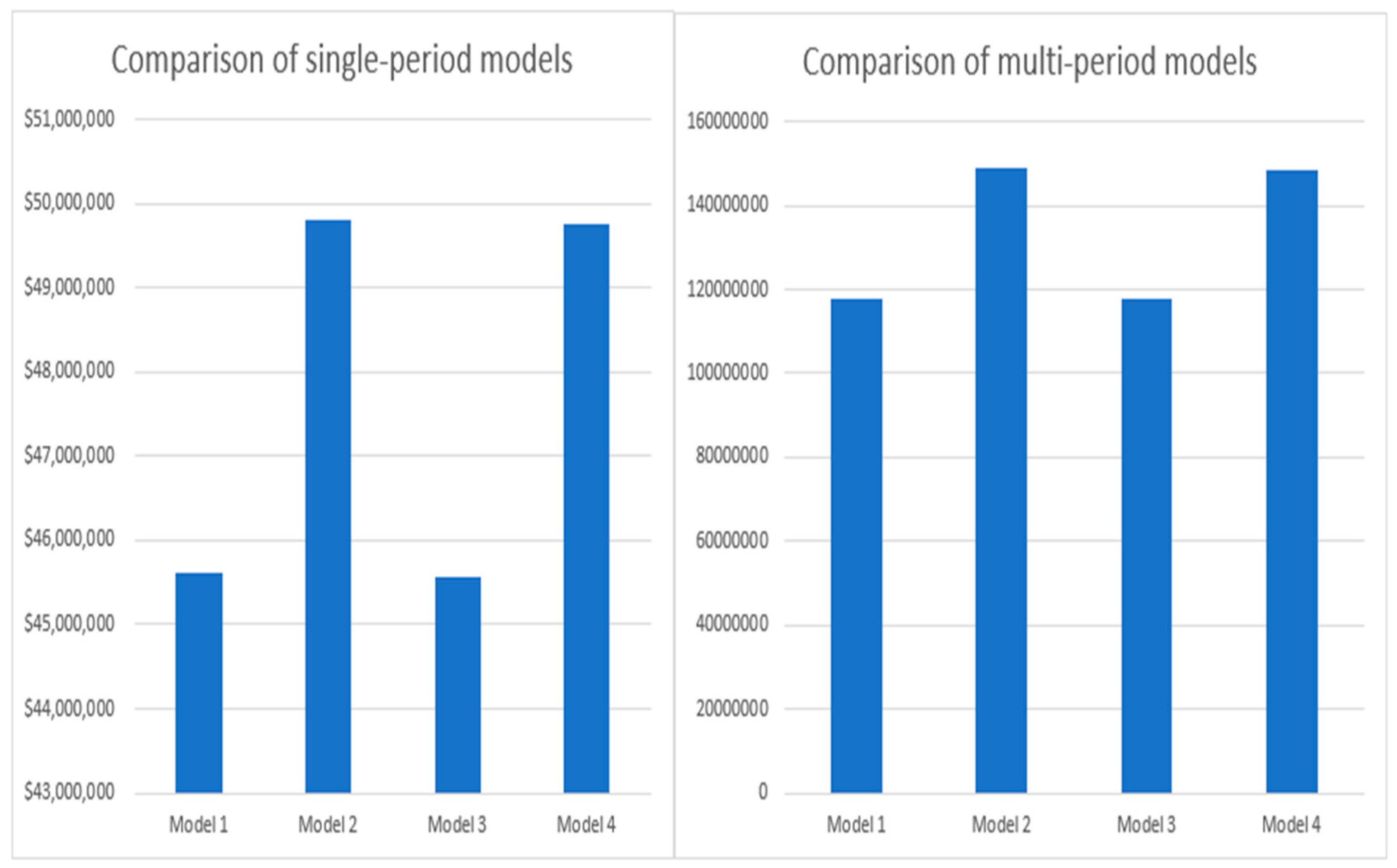
4.2.2. Comparison of Single-Period and Multi-Period Models

This section compares the results of single-period (Table 7) and multi-period (Table 8) models. From the results of the single-product models (Table 7), models with carbon trading (Models 2 and 4) have higher profits than those without (Models 1 and 3). Model 2 (continuous carbon tax with trading) has the highest profit at TWD 49,807,842.

The results of the single-product models (Table 7) are described below:

As for product output, models with carbon trading produce more X3 to meet demand. Models 2 and Model 4 have the same output mix. Regarding carbon emissions, models with carbon trading have higher emissions (272,109 kg) than those without (249,999 kg). With respect to carbon tax cost, discontinuous tax models (Model 3 and Model 4) have higher costs than continuous models (Model 1 and Model 2). Regarding labor hours, models with carbon trading require more labor, including overtime, because of the higher product output needed. Concerning batch-level costs, models with carbon trading have slightly higher forming, setting, and handling costs.

The results of the multi-period models (Table 8) are described below:

The results of multi-product cases are shown in Table 8. Regarding profit, continuous tax models (Model 1 and Model 2) have higher profits than discontinuous models (Model 3 and Model 4). Model 2 has the highest profit at TWD 148,742,200 across all periods. Regarding product output, production varies by period based on carbon constraints and pre-borrowing/storing. Models with trading generally produce more X3. Concerning carbon emissions, emissions fluctuate as companies strategically allocate or bank emissions. Models with trading have higher total emissions. With respect to carbon tax cost, discontinuous tax models have higher total costs than continuous models. Regarding pre-borrowing or storing emissions, only continuous tax models (Model 1 and Model 2) allow this across periods. With respect to labor hours, requirements vary by period based on production, with trading models generally requiring more hours. Figure 5 shows the profit comparisons across the models in the single-period and multi-period cases.

5. Discussion and Conclusions

5.1. Discussion

This study stands out from others in the scientific literature by comprehensively integrating activity-based costing (ABC), the theory of constraints (TOC), and carbon emission costs within the framework of Industry 4.0. Unlike previous studies that often examine these elements in isolation, this research proposes a holistic approach that combines cost control, profit optimization, and environmental sustainability. The results indicate that continuous carbon tax models, especially those incorporating carbon trading mechanisms, offer significant advantages in balancing profitability and emissions reduction. This study also highlights the operational flexibility provided by carbon trading, enabling more effective production scheduling and labor cost management. By comparing the total revenue and detailed costs, it becomes clear that fixed costs, such as equipment depreciation, rent, and salaries, remain constant and provide financial stability. In contrast, variable costs, including raw materials and direct labor, fluctuate with production levels and impact profitability. For the analyzed company, fixed costs offer greater predictability and stability, which is beneficial for long-term financial planning.

5.2. Conclusions

The findings indicate that integrating carbon trading mechanisms can significantly enhance profitability while achieving environmental goals. Continuous carbon tax models, particularly those with trading options, appear to offer the most balanced approach for maximizing profits and minimizing emissions. For instance, Model 2 shows that carbon trading can mitigate the financial impact of carbon taxes, making it a viable strategy for companies aiming to balance economic and environmental objectives. Additionally, lowering emission caps proves more effective in curbing emissions than merely increasing tax rates. Policymakers should consider these insights when designing carbon tax and carbon emission trading programs to drive industrial transition toward a low-carbon economy. This study contributes to sustainable operations management by providing a robust framework that integrates cost control, profit optimization, and environmental sustainability within the context of Industry 4.0. The use of advanced technologies and data analytics can further enhance the effectiveness of such integrated models, supporting more informed and strategic decision-making. Future research should focus on refining the models under more realistic constraints and exploring their application in various industries. Enhancing dynamic adjustment algorithms can further emphasize the balance between profitability and environmental sustainability, aiding industry leaders and policymakers in promoting sustainable manufacturing practices and contributing to broader goals of mitigating climate change impacts. One limitation of our study is that it focuses solely on the knitted shoe manufacturing industry. The results may not be directly applicable to other sectors with different production dynamics and regulatory environments.

References

1. Bockorny, M.; Raber, M.; Vos, Y. The use of Dimethylformamide (DMF) in the shoe production and its effects on health and environment. RIVM Lett. Rep. 2017, 2017, 136. [Google Scholar] [CrossRef]
2. Ellen MacArthur Foundation. A New Textiles Economy: Redesigning Fashion’s Future. Available online: https://www.ellenmacarthurfoundation.org/assets/downloads/publications/A-New-Textiles-Economy_Full-Report_Updated_1-12-17.pdf (accessed on 1 July 2024).
3. Moretto, A.; Macchion, L.; Lion, A.; Caniato, F.; Danese, P.; Vinelli, A. Designing a roadmap towards a sustainable supply chain: A focus on the fashion industry. J. Clean. Prod. 2018, 193, 169–184. [Google Scholar] [CrossRef]
4. Bianchi, I.; Forcellese, A.; Simoncini, M.; Vita, A.; Castorani, V.; Cafagna, D.; Buccoliero, G. Comparative life cycle assessment of safety shoes toe caps manufacturing processes. Int. J. Adv. Manuf. Technol. 2022, 120, 7363–7374. [Google Scholar] [CrossRef]
5. Ghimouz, C.; Kenné, J.P.; Hof, L.A. On sustainable design and manufacturing for the footwear industry–Towards circular manufacturing. Mater. Des. 2023, 233, 112224. [Google Scholar] [CrossRef]
6. Caniato, F.; Caridi, M.; Crippa, L.; Moretto, A. Environmental sustainability in fashion supply chains: An exploratory case based research. Int. J. Prod. Econ. 2012, 135, 659–670. [Google Scholar] [CrossRef]
7. Dissanayake, G.; Sinha, P. An examination of the product development process for fashion remanufacturing. Resour. Conserv. Recycl. 2015, 104, 94–102. [Google Scholar] [CrossRef]
8. Lee, M.J.; Rahimifard, S. An air-based automated material recycling system for postconsumer footwear products. Resour. Conserv. Recycl. 2012, 69, 90–99. [Google Scholar] [CrossRef]
9. Bhavan, S.; Rao, J.R.; Nair, B.U. A potential new commercial method for processing leather to reduce environmental impact. Environ. Sci. Pollut. Res. 2008, 15, 293–295. [Google Scholar] [CrossRef]
10. Chen, K.W.; Lin, L.C.; Lee, W.S. Analyzing the carbon footprint of the finished bovine leather: A case study of aniline leather. Energy Proc. 2014, 61, 1063–1066. [Google Scholar] [CrossRef]
11. Kılıç, E.; Puigb, R.; Zengin, G.; Zengin, C.A.; Fullana-I-Palmer, P. Corporate carbon footprint for country climate change mitigation: A case study of a tannery in Turkey. Sci. Total Environ. 2018, 635, 60–69. [Google Scholar] [CrossRef] [PubMed]
12. Milà I Canals, L.; Domènèch, X.; Rieradevall, J.; Puig, R.; Fullana, P. Use of life cycle assessment in the procedure for the establishment of environmental criteria in the catalan eco-label of leather. Int. J. Life Cycle Assess. 2002, 7, 39–46. [Google Scholar] [CrossRef]
13. Bodoga, A.; Nistorac, A.; Loghin, M.C.; Isopescu, D.N. Environmental Impact of Footwear Using Life Cycle Assessment—Case Study of Professional Footwear. Sustainability 2024, 16, 6094. [Google Scholar] [CrossRef]
14. Perdijk, E.W.; Luijten, J.; Selderijk, A.J. An Eco-Label for Footwear. Background Report (Report Number: 9041); CEA, Communication and Consultancy on Environment and Energy, Centrum TNO Leather and Shoes: Rotterdam, The Netherlands, 1994. [Google Scholar]
15. Van Rensburg, M.L.; Nkomo SP, L.; Mkhize, N.M. Life cycle and End-of-Life management options in the footwear industry: A review. Waste Manag. Res. 2020, 38, 599–613. [Google Scholar] [CrossRef] [PubMed]
16. Gottfridsson, M.; Zhang, Y. Environmental Impacts of Shoe Consumption—Combining Product Flow Analysis with an LCA Model for Sweden; Department of Energy and Environment, Division of Environmental Systems Analysis, Chalmers University of Technology: Gothenburg, Sweden, 2015. [Google Scholar]
17. Bhat, R.A.; Dervash, M.A.; Mehmood, M.A.; Hakeem, K.R. Municipal solid waste generation and its management a growing threat to fragile ecosystem in Kashmir Himalaya. Am. J. Environ. Sci. 2017, 13, 388–397. [Google Scholar] [CrossRef]
18. Kazuva, E.; Zhang, J. Analyzing municipal solid waste treatment scenarios in rapidly urbanizing cities in developing countries: The case of Dar es Salaam, Tanzania. Int. J. Environ. Res. Public Health 2019, 16, 2035. [Google Scholar] [CrossRef] [PubMed]
19. Oelofse, S.H.H.; Nahman, A. Waste production and disposal in South Africa. Environ. Sci. Policy 2019, 94, 46–56. [Google Scholar]
20. O’Neill, K. The global environmental injustice of fast fashion. Environ. Health 2018, 17, 92. [Google Scholar] [CrossRef]
21. Ozc1an, K.; Suthar, S.; Singh, S. Household waste categorization and its environmental impact: A comprehensive analysis. Waste Manag. 2016, 56, 234–245. [Google Scholar]
22. Behrendt, G.; Naber, B.W. The chemical recycling of polyurethanes. J. Chem. Technol. Metall. 2009, 44, 3–23. [Google Scholar]
23. Chrobot, P.; Faist, M.; Gustavus, L.; Martin, A.; Stamm, A.; Zah, R.; Zollinger, M. Measuring Fashion: Environmental Impact of the Global Apparel and Footwear Industries Study; Quantis. Available online: https://quantis.com/report/measuring-fashion-report/ (accessed on 1 July 2024).
24. World Footwear Yearbook 2023. Global Footwear Production Reaches 23.9 Billion Pairs and Is Back to Pre-Pandemic Levels. Retrieved from World Footwear. Available online: https://www.worldfootwear.com/news/2022-global-footwear-production-reaches-239-billion-pairs-back-to-pre-pandemic-levels/9025.html (accessed on 1 July 2024).
25. Mwinyihija, M. An analysis of the synthetic leather footwear industry in Kenya. J. Clean. Prod. 2018, 196, 953–960. [Google Scholar]
26. Cheah, L.; Ciceri, N.D.; Olivetti, E.; Matsumura, S.; Forterre, D.; Roth, R.; Kirchain, R. Manufacturing-focused emissions reductions in footwear production. J. Clean. Prod. 2013, 44, 18–29. [Google Scholar] [CrossRef]
27. Wang, Z.; Wang, L.H. Low-carbon economic development under carbon emission trading system—Analysis based on non-expected DEA and DID model. J. Southwest Univ. 2019, 41, 85–95. [Google Scholar] [CrossRef]
28. Verde, S.F. The impact of the EU emissions trading system on competitiveness and carbon leakage: The econometric evidence. J. Econ. Surv. 2020, 34, 320–343. [Google Scholar] [CrossRef]
29. Lin, T.J.; Wang, J.S.; Hsieh, P.H.; Hsu, T.S. Advantage analysis and integration planning of Taiwan carbon trading platform. Qtly. J. Bus. Manag. 2015, 16, 269–289. [Google Scholar]
30. Albino, V.; Ardito, L.; Dangelico, R.M.; Petruzzelli, A.M. Understanding the development trends of low-carbon energy technologies: A patent analysis. Appl. Energy 2014, 135, 836–854. [Google Scholar] [CrossRef]
31. De Marchi, V. Environmental innovation and R&D cooperation: Empirical evidence from Spanish manufacturing firms. Res. Policy 2012, 41, 614–623. [Google Scholar] [CrossRef]
32. Yan, Z.; Yi, L.; Du, K.; Yang, Z. Impacts of low-carbon innovation and its heterogeneous components on CO2 emissions. Sustainability 2017, 9, 548. [Google Scholar] [CrossRef]
33. Yin, H.; Zhao, J.; Xi, X.; Zhang, Y. Evolution of regional low-carbon innovation systems with sustainable development: An empirical study with big-data. J. Clean. Prod. 2019, 209, 1545–1563. [Google Scholar] [CrossRef]
34. Borghesi, S.; Cainelli, G.; Mazzanti, M. Linking emission trading to environmental innovation: Evidence from the Italian manufacturing industry. Res. Policy 2015, 44, 669–683. [Google Scholar] [CrossRef]
35. Calel, R.; Dechezlepretre, A. Environmental policy and directed technological change: Evidence from the European carbon market. Rev. Econ. Stat. 2016, 98, 173–191. [Google Scholar] [CrossRef]
36. Kim, W.; Yu, J. The effect of the penalty system on market prices in the Korea ETS. Carbon Manag. 2018, 9, 145–154. [Google Scholar] [CrossRef]
37. Luthra, S.; Mangla, S.K. Evaluating the impact of industry 4.0 on supply chain sustainability. Proc. Manuf. 2018, 21, 563–570. [Google Scholar]
38. Kiel, D.; Müller, J.M.; Arnold, C.; Voigt, K.I. Sustainable industrial value creation: Benefits and challenges of industry 4.0. Int. J. Innov. Manag. 2017, 21, 1740015. [Google Scholar] [CrossRef]
39. Dalenogare, L.S.; Benitez, G.B.; Ayala, N.F.; Frank, A.G. The expected contribution of industry 4.0 technologies for industrial performance. Int. J. Prod. Econ. 2018, 204, 383–394. [Google Scholar] [CrossRef]
40. Gabriel, M.; Pessl, E. Industry 4.0 and sustainability impacts: Critical discussion of sustainability aspects with a special focus on future of work and ecological consequences. Ann. Fac. Eng. Hunedoara 2016, 14, 131–136. [Google Scholar]
41. Müller, J.M.; Kiel, D.; Voigt, K.I. What drives the implementation of industry 4.0? The role of opportunities and challenges in the context of sustainability. Sustainability 2018, 10, 247. [Google Scholar] [CrossRef]
42. de Sousa Jabbour, A.B.L.; Jabbour, C.J.C.; Foropon, C.; Godinho Filho, M. When titans meet—Can industry 4.0 revolutionise the environmentally-sustainable manufacturing wave? The role of critical success factors. Technol. Forecast. Soc. Change 2018, 132, 18–25. [Google Scholar] [CrossRef]
43. Beltrami, M.; Orzes, G. A systematic review of industry 4.0 and sustainability. In Proceedings of the 2019 IEEE International Conference on Engineering, Technology and Innovation (ICE/ITMC), Valbonne, France, 17–19 June 2019; pp. 1–9. [Google Scholar]
44. Park, J.; Sarkis, J.; Wu, Z. Creating integrated business and environmental value within the context of China’s circular economy and ecological modernization. J. Clean. Prod. 2010, 18, 1494–1501. [Google Scholar] [CrossRef]
45. Cooper, R.; Kaplan, R.S. Activity-based costing: Introducing a new cost management system. J. Cost Manag. 1988, 2, 4–15. [Google Scholar]
46. Kim, G.; Ballard, G. Applying ABC to construction projects. J. Constr. Eng. Manag. 2001, 127, 176–185. [Google Scholar]
47. Fichman, M.; Kemerer, C.F. Software development: Using ABC for cost management. Inform. Syst. Res. 2002, 13, 267–283. [Google Scholar]
48. AlMaryani, M.A.K.; Sadik, Z. Environmental protection costs: Insights from the ABC method. Environ. Resour. Econom. 2012, 52, 549–564. [Google Scholar]
49. Goldratt, E.M.; Cox, J. The Theory of Constraints and Its Implications for Management Accounting; The North River Press: Great Barrington, MA, USA, 1984. [Google Scholar]
50. Tsai, W.H.; Jhong, S.Y. Production decision model with carbon tax for the knitted footwear industry under activity-based costing. J. Clean. Prod. 2019, 207, 1150–1162. [Google Scholar] [CrossRef]
51. Hsieh, C.L.; Tsai, W.H. Sustainable Decision Model for Circular Economy towards Net Zero Emissions under Industry 4.0. Processes 2023, 11, 3412. [Google Scholar] [CrossRef]
Figure 1. Knitted shoe manufacturing process.
Sustainability 16 07120 g001
Figure 2. The carbon tax cost function.
Sustainability 16 07120 g002
Figure 3. Carbon tax cost function of discontinuous.
Sustainability 16 07120 g003
Figure 4. Direct labor cost equation.
Sustainability 16 07120 g004
Figure 5. Model comparison profit (by TWD).
Sustainability 16 07120 g005