Abstract
Public debt plays a major role in financing projects that support economic growth and sustainable development. As governments may choose between domestic and external borrowing, a comprehensive assessment of their effects would support this choice. Our study provides an integrative view of economic and social outcomes and compares, through externalities, the impacts of external and domestic public debt as methods of financing development, with a focus on the Cameroonian economy. Utilizing a dynamic computable general equilibrium (CGE) model and a microsimulation analysis, we find that domestic debt has more advantages for Cameroon compared to external debt, as it increases the large-scale economic impact by improving household welfare, boosting GDP growth, and progressively reducing poverty and inequality. It is therefore recommended that the Cameroonian government focus on increasing the use of domestic debt as a method of financing development by implementing policies that support domestic saving and promote the development of domestic debt markets.
1. Introduction
In many countries, public debt plays a significant role in financing development by providing the necessary funds for investment in infrastructure, education, healthcare, social welfare programs, and other development projects. Particularly in developing economies, where the development needs are high but the fiscal systems are severely strained and resources are scarce, public debt serves as a crucial source of financing for initiatives aimed at promoting economic growth, reducing poverty, and improving the living standards of citizens, as recent studies suggest [1,2]. Nevertheless, the relationship between debt and development is one between friends and foes; debt mismanagement, excessive borrowing, and debt accumulation may pose substantial risks to macroeconomic stability and hinder future development efforts [3,4].
In Cameroon, as in many other developing economies, public debt was used as a tool for mobilizing additional resources and supporting growth. Up to the beginning of the 1980s, Cameroon practiced a prudent debt policy, and the increase in external debt, although continuous, led to only moderate debt levels compared to similar countries. Nevertheless, starting in the mid-1980s, the situation changed. Cameroon faced serious cash deficits and devalued the CFA franc to stimulate exports and restore budget balance, while the bulk of its debt was denominated in foreign currency. However, the expected positive effects were not observed, and external debt increased steadily and more than tripled over the following decade. In 1996, the Bretton Woods institutions launched the Heavily Indebted Poor Countries (HIPC) initiative to alleviate the debt burden of developing countries. Cameroon joined this initiative and reached the completion point in 2005, benefiting from a reduction in its debt. In 2020, the country was granted a moratorium on its debt because of the COVID-19 pandemic. The G20’s debt-suspension initiative allowed Cameroon to postpone the payment of $108 million in external debt in 2020 [5]. Such initiatives as HIPC and IMF interventions are tools used to help developing countries cope with their economic difficulties and reduce their debt. At present, although public debt is well below the 70% of GDP threshold set as a convergence criterion by CEMAC (Central African Economic and Monetary Community) member states, Cameroon is facing a high risk of debt distress. This underscores the high importance of prudent debt management and the appropriate choice of future sources of funding to avoid unfavorable debt developments while also allowing the government to reach a wide range of economic and social goals.
The economy of a developing country like Cameroon is therefore faced with a complex dilemma when it comes to financing economic initiatives and supporting development. One of the core questions is whether the government should rely on foreign or domestic debt to finance its projects. This decision is not simply a matter of weighing the pros and cons but also requires an in-depth analysis of the economic and social externalities associated with each option.
Theory suggests that both external and domestic debt may have advantages and disadvantages. External debt allows for rapid access to substantial financial resources, enabling the financing of large-scale infrastructure and development projects [6,7]. It also makes it possible to benefit from the foreign knowledge and expertise needed to implement these projects effectively [8]. However, external debt can also lead to economic dependence on foreign creditors, with potential implications for national sovereignty and economic policy [9]. Alternatively, domestic debt offers a higher degree of independence and economic control, as the government can mobilize financial resources internally, mainly by issuing bonds [10]. This allows it to diversify its sources of finance and make more autonomous development decisions [11,12]. However, excessive reliance on domestic debt can also lead to an accumulation of unsustainable debt, inflation, and higher interest rates, which in turn can undermine economic stability and investor confidence [13,14].
In recent years, the effects of overall public or external debt in developing economies have been extensively investigated, with most of the studies focusing on the debt-growth nexus in one individual country or a group of countries. While some researchers looked at the direct effects of debt on economic growth or identified a debt threshold [15,16,17,18,19,20], others focused on the factors moderating debt’s impact on growth, like the liquidity of the economy [21], the stability of macroeconomic policies [22], or the quality of institutions [18]. With regard to domestic public debt, a few studies focused on crowding-out effects and investigated its impact on private investment [23] or corporate debt [24]. All these studies have contributed to our understanding of public debt issues and clearly emphasized the importance of domestic and external debt in financing development. Nevertheless, without disregarding the contribution of growth-focused studies, we appreciate that they offer an incomplete picture of the complex network of effects linking government debt financing to development.
Against this background, our study aims to comparatively assess, through externalities, the impacts of external and domestic government debt as methods of financing development in Cameroon. While reaching economic goals is of high importance to developing countries, we advocate for a wider approach that integrates economic and social considerations when choosing the appropriate source of funding. Therefore, we combine macroeconomic and microeconomic approaches to simulate the long-term effects of an increase in Cameroon’s foreign and domestic debt on various economic and social indicators such as production, prices, household welfare, income inequality, and poverty.
This study stands out in several respects. First, it offers an integrative and comparative approach to the impact of external and domestic public debt on Cameroon’s development. Unlike previous research that focuses primarily on the effects of debt on economic growth, our work takes a broader perspective by examining the economic and social impacts associated with each type of debt. Second, we consider economic and social externalities in the analysis, which are essential to assessing the indirect effects of financing choices on an economy. In particular, external debt can contribute to an increase in imports of goods and services, which may have a negative impact on the balance of trade [25]. Moreover, domestic debt can affect the availability of bank loans for the private sector, which may hamper investment and economic growth in the long run [26]. Third, by using a dynamic computable general equilibrium (CGE) model coupled with a microsimulation analysis, we are able to capture the complex interactions between different sectors of the economy and estimate the long-term sectoral and social impacts of financing choices. This innovative methodology not only assesses the direct effects of debt on economic growth but also emphasizes the indirect consequences on income distribution, poverty, and inequality.
By focusing on the specific case of Cameroon, this study provides empirical support for concrete policy recommendations that are tailored to local realities. Therefore, our research could be useful to public authorities in Cameroon for designing debt strategies that maximize the positive effects of government interventions. In addition, our study opens perspectives that are applicable to other developing countries. Cameroon’s situation in terms of public debt, whether foreign or domestic, is relevant not only for the country itself but also for the international community. As a developing country with a diversified economy and abundant natural resources, Cameroon represents a relevant case study for understanding debt dynamics and its impact on economic development, and the lessons learned from the Cameroonian experience can be applied to other developing countries facing similar economic conditions and development financing challenges. By exploring the externalities associated with public debt, this study contributes to a broader debate on sustainable development financing strategies, offering valuable insights for international financial institutions, and policymakers and researchers in all developing countries.
The structure of this paper is as follows: we begin by briefly presenting some facts about Cameroon’s external and domestic debt dynamics in Section 2; in Section 3, we review the existing literature to explore the potential effects of different indebtedness options; in Section 4, we describe the methodological approach; Section 5 presents the results and discusses their implications; and finally, in Section 6, we conclude by summarizing the main results and identifying policy implications and recommendations for the choice of financing for Cameroon’s development.
2. Overview of Cameroon’s Foreign and Domestic Debt Trends
In this section, we briefly explore the evolution of Cameroon’s debt. The data in Figure 1 give us valuable insights into external and domestic debt fluctuations over the period 2000–2021, in both nominal and relative terms. When distinguishing between domestic and foreign debt, we consider the criterion of creditors’ residence; therefore, domestic debt refers to the government borrowing from domestic creditors, while external debt refers to borrowing from foreign creditors.
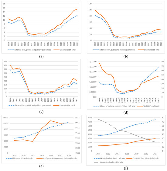
Figure 1.
External and domestic debt indicators for Cameroon (data from: the World Bank, World Development Indicators database, https://databank.worldbank.org/source/world-development-indicators, (accessed on 15 March 2024); IMF, World Economic Outlook database, https://www.imf.org/en/Publications/WEO/weo-database/2023/October, (accessed on 15 March 2024); and the Ministry of Finance of Cameroon, https://minfi.gov.cm/category/documentation/, (accessed on 15 March 2024)). (a) External debt (in billions of current $); (b) External debt/GDP ratio (%); (c) External debt/Exports ratio (%); (d) General government debt; (e) Central government debt; (f) Domestic and external central government debt (in billions of FCFA).
The total stock of external debt increased from $10.6 billion in 2000 to $15.4 billion in 2021 (Figure 1a). Nevertheless, this general trend hides changing dynamics over the years. External debt decreased up to 2005, given the government’s efforts to reduce the debt burden and improve the country’s economic situation. A sharp decrease was further registered in 2006, followed by a slight decline between 2006 and 2011 because of the commitments undertaken and support granted by international creditors under the enhanced HIPC. Nevertheless, from 2011 to 2021, external debt grew significantly because of increased external borrowing to finance infrastructure projects or cover budget deficits.
The overall rise in the country’s external debt over the years resulted mostly from additional government liabilities. External public and publicly guaranteed debt closely followed the trend of total external debt, rising from $8.8 billion in 2000 to $12.4 billion in 2021. Nevertheless, the external debt/GDP ratio dropped from 99.9% in 2000 to 34.2% in 2021, with most of the decrease being registered up to 2011, when external debt recorded a minimum of 6.9% of GDP. Over the same period (2000–2021), external public and publicly guaranteed debt decreased from 82.8% to 27.5% of GDP (Figure 1b). Moreover, following the same trend, the debt-to-exports ratio fell from 402.1% in 2000 to 206.9% in 2021, at about half its value in 2000 (Figure 1c).
The analysis of overall public debt data also reveals some important trends over the years (Figure 1d). Cameroon’s general government debt/GDP ratio decreased from 75.9% in 2000 to a minimum of 11.2% of GDP in 2008 and then increased continuously to 46.8% in 2021 because of the decline in oil revenues, the security crisis, the COVID-19 pandemic, and investment needs in infrastructure. Central government debt represents the bulk of this debt, accounting for about 90% of the total amount (Figure 1e). In addition, over the period 2015–2021, domestic debt represented no more than 30% of central government debt (Figure 1f), which emphasizes that foreign creditors are the main providers of funds to the Cameroonian government, which preferred to finance its projects by borrowing externally. Nevertheless, despite the quite similar patterns that domestic and external debt exhibited in recent years, both increasing because of the high financing requirements of the government or the late payments to external creditors, the contribution of domestic creditors slightly improved after 2018. The ratio of domestic debt to overall central government debt rose from 23.7% in 2018 to 28.1% in 2021, which highlights an increased interest in using domestic markets as an alternative to external creditors.
Overall, this brief analysis shows the significant efforts of the government to strike a balance between external and domestic borrowing while focusing on prudent debt management to ensure long-term economic stability. Moreover, it points to an increasing role of domestic creditors as financial resource providers for the government, which substantiates the need for an in-depth comparative analysis of domestic and external debt’s effects.
3. Theoretical Background and Empirical Literature
Financing development through public debt is a major concern for governments and economists in developing countries. In time, several economic theories have been put forward to understand the economic and political aspects of public debt, each making equally important contributions. In addition, many empirical studies explored economic and political factors such as trade balances, exchange rates, interest rates, economic size, and institutional factors to understand how developing countries manage their public debt.
Grounding their arguments on Keynes’ most influential work [27], Keynesian economists emphasize the positive role of public debt in supporting fiscal policy interventions to stabilize the economy and promote full employment. In times of recession, when aggregate demand falls short of aggregate supply, increased government spending or tax cuts financed through government borrowing may spur economic activity and resume economic growth. Nevertheless, the crowding-out theory (that Keynes himself brought forward but subsequent monetarist economists refined) argues that such positive effects may not occur or be smaller than expected, as an increase in public debt can lead to an increase in interest rates, which further reduces private investment and slows down economic growth.
Developed by Krugman [28], the debt cycle theory further suggests that developing countries can enter a vicious cycle of indebtedness, in which they borrow to repay their existing debt, leading to a continuous increase in debt. Stiglitz’s creditor response theory [29] argues that the conditions and policies imposed by international creditors can have a significant impact on the level of public debt. According to this theory, creditors can influence the economic policies of developing countries according to their interests.
Reinhart and Rogoff’s theory of the costs of debt reduction [30] highlights the negative effects of decreasing public debt. According to this theory, efforts to cut down on debt can lead to high social costs, such as reduced social spending, which can harm the population.
Finally, the theory of debt solutions proposes various strategies for dealing with the problem of public debt, such as debt renegotiation, restructuring, and debt forgiveness. This theory emphasizes the need to find viable political and economic solutions to the debt crisis. The key authors of this theory include several economists and researchers specializing in the field of development economics, notably those mentioned above.
These theories have given rise to a vast empirical literature on the effects of public debt. Whether external or domestic, public debt is a major concern for many developing countries, as it can have a significant impact on economic growth, macroeconomic stability, and social welfare. However, the impact of public debt on development is ambiguous and depends on several factors, such as the level, composition, maturity, cost, and sustainability of the debt, in addition to the institutional, political, and economic context of the country. The empirical literature on this topic is rich and diverse, but also sometimes contradictory and incomplete. In this review, we briefly present the main findings and limitations of existing studies, grouping them along three axes: the impact of public debt on growth, the impact of external debt on growth, and the impact of domestic debt on growth.
Public debt is a topic that generates much debate in the economic literature, particularly concerning its impact on economic growth. Several empirical studies have tried to measure this effect using different methods and data. We can distinguish two main approaches: one that considers the relationship between public debt and economic growth to be linear and negative, and the other that states the relationship is nonlinear and depends on the level of public debt and further identifies the threshold at which the relationship between public debt and economic growth/development reverses.
The linear approach assumes that public debt has a negative effect on economic growth, regardless of its level. This hypothesis is based on the theory of crowding out, according to which an increase in public debt leads to an increase in interest rates, which further reduces private investment and aggregate demand. It also draws on the theory of odious debt, which states that public debt can be considered illegitimate if it is not used to finance productive expenditures or if it is contracted by corrupt or authoritarian regimes. Studies using this approach include Refs. [16,31]. Based on panel data from developed and emerging economies, these find an inverse and linear relationship between public debt and economic growth. In other words, the more public debt increases, the more economic growth decreases. More recently, similar findings have been confirmed for a group of 45 sub-Saharan African countries by Sumba et al. [32], who also presented evidence of a negative effect of public debt on macroeconomic stability and inflation. For a smaller group of just 11 sub-Saharan African economies, Obiero and Topuz [33] investigated the causal relationships between public debt, economic growth, and income inequality and found that these vary according to the specific characteristics of the countries.
The nonlinear approach is based on the assumption that the relationship between public debt and economic growth is not constant but varies with the level of public debt. This hypothesis is based on the critical threshold theory, according to which public debt has no significant effect on economic growth as long as it remains below a certain threshold but becomes detrimental beyond this threshold. It is also based on the theory of the inverted U-curve, which states that public debt can have a positive effect on economic growth at moderate levels by financing productive public spending, but it becomes negative at higher levels by creating fiscal distortions and uncertainty. Among the studies using this approach, Ref. [34] examined data from 44 countries over two centuries and found that there was no apparent relationship between public debt and economic growth up to a threshold of 90% of GDP. Beyond this threshold, economic growth slows down significantly. Checherita-Westphal and Rother [35] examined a sample of Eurozone countries over the period 1970–2009. Their results showed that when public debt exceeds 90% of GDP, it weakens economic growth. Below this threshold, however, the relationship between debt and growth is insignificant. A study by Caner et al. [15] confirmed these results, based on data from 101 developed and developing countries between 1980 and 2008. They also found a nonlinear relationship between public debt and economic growth. Similarly, the study by Cecchetti et al. [36] on a sample of 18 OECD countries between 1980 and 2010 identified a threshold of 85% of GDP that should not be exceeded to avoid the negative impact of public debt on economic growth. Da Veiga et al. [37] found evidence in a group of 52 African countries that there is an inverted-U relationship between public debt and economic growth, while high public debt levels are also associated with more inflation. Finally, Presbitero [38] examined the impact of public debt on growth in developing countries, focusing on the expansionary response of governments to the global crisis. His results showed that public debt has a negative impact on growth at the threshold of 90% of GDP, beyond which the effects are no longer significant. This non-linear effect is explained by country-specific factors, with excessive debt being a constraint on growth only in countries with sound macroeconomic policies and stable institutions. Other studies confirm that there is high cross-country heterogeneity in the public debt–economic growth nexus, with the relationship depending on various factors, among which are the income level [39,40] or type of economic system [41].
Regarding the impact of external debt on growth, foreign debt is often seen as a means of financing development, which allows countries to import capital goods, undertake public investment, finance budget deficits, and support domestic demand. However, external debt can also have negative effects on growth by creating distortions in the allocation of resources, reducing the availability of credit, increasing vulnerability to external shocks, inducing opportunistic or strategic behavior by debtors and creditors, and restricting fiscal space and economic policy’s room for maneuver. Several empirical studies have attempted to measure the impact of external debt on growth using various econometric techniques such as threshold models, error correction models, instrumental variable models, impact models, fixed or random effects models, or dynamic panel data models. These studies have generally found that there is a nonlinear relationship between external debt and growth, i.e., above a certain threshold, external debt becomes detrimental to growth. However, the level of this threshold varies across studies, ranging from 20% to 90% of GDP, depending on the indicators, periods, samples, and specifications used. For example, Pattillo et al. [42] estimated that the threshold is between 35% and 40% of GDP for low-income countries and between 15% and 20% of GDP for middle-income countries. Reinhart and Rogoff [30] proposed a higher threshold of 60% of GDP, above which the average growth rate falls by more than one percentage point. In the study of Lau et al. [20], the threshold varies for different groups of Asian developing countries, between below 30% of GDP and 60%–90% of GDP. Moreover, the growth effects are not limited to one country, but significant spillovers may occur, especially at the regional level. Examining the impact of geographic proximity and spatial spillovers on public debt and economic growth dynamics in East Africa over the period 1992–2019, Otieno [43] found evidence that foreign public debt has a negative impact on economic growth, which is consistent with the debt overhang theory and the crowding-out hypothesis. In addition, along with many other macroeconomic variables, foreign debt is found to have significant spatial spillover effects on regional economic growth. A separate strand of research has highlighted the importance of the quality of institutions, fiscal policy, degree of openness, exchange rate, and type of creditors as moderating or amplifying factors in the impact of external debt on economic growth. For example, Dey and Tareque [22] found that external debt has a positive effect on growth when macroeconomic policies are stable but a negative effect when policies are unstable. Ehigiamusoe and Lean [44] found that macroeconomic stability and institutional quality foster financial development, which in turn enhances the positive effect of external debt on growth. Moshin et al. [18] emphasized that better institutions can help alleviate the negative effects of external debt on economic growth.
As several studies indicate, the foreign currency denomination of external debt is particularly important for shaping its economic and developmental effects. Grounding their demonstration on a two-country New Keynesian DSGE model with nominal rigidities and financial frictions, Hory et al. [45] demonstrated that foreign currency debt can influence domestic financial conditions. They showed that the increase in the burden of foreign currency-denominated debt issued to finance public spending deteriorates the balance sheets of domestic firms by increasing their external financing premium and crowding out private investment, ultimately offsetting the positive effect of the government spending shock. Furthermore, Lu et al. [46] found that the composition of foreign exchange reserves may be altered, with higher proportions of dollar-denominated external debt leading central banks to hold more U.S. dollars. Coulibaly et al. [47] also provided evidence on the buffering effects of international reserves in Africa, which is crucial for understanding debt management mechanisms. Finally, Apeti et al. [48] discussed the role of fiscal rules in limiting foreign currency debt and exposure to the problem of “original sin” in developing countries.
Domestic debt, i.e., public debt held by the residents of a country, is often perceived as less risky and more flexible than external debt because it is not dependent on international market conditions, does not involve a transfer of resources abroad, does not create currency mismatch problems, and can be renegotiated or restructured more easily. However, domestic debt can also have negative effects on growth by crowding out the private sector, increasing financing costs, reducing the effectiveness of monetary policy, creating inflationary expectations, and introducing fiscal distortions. Empirical studies on the impact of domestic debt on growth are fewer and less consistent than those on external debt, due to the difficulty of obtaining reliable and comparable data on domestic debt and the complexity of isolating its effect from other factors. Some studies have found a negative effect of domestic debt on growth using threshold models, error correction models, or panel data models. For example, Abbas and Christensen [49] estimated that the threshold is between 35% and 40% of GDP for emerging economies and between 70% and 80% of GDP for advanced economies. Kumar and Woo [31] found a lower threshold of 30% of GDP for the OECD countries. Other studies evidenced a positive or insignificant effect of domestic debt on growth using instrumental variable models, fixed or random effects models, or dynamic panel data models. For example, Panizza [50] found that domestic debt has no significant effect on growth but reduces the likelihood of external debt crises. Presbitero [51] emphasized that domestic debt has a positive effect on growth, but this effect is weaker than that of external debt. Ehigiamusoe and Samsurijan [52] noted that the effect of domestic debt on growth depends on the quality of institutions, fiscal policy, and the degree of financial development.
The banking sector may be an important player in providing domestic resources to governments and supporting economic growth, especially in developing countries. According to Presbitero [38], local banks can contribute to financial stability by diversifying their portfolios with public debt securities, thereby reducing their exposure to the risks associated with private lending. This interaction between the banking sector and public debt can also stimulate the economy by increasing liquidity and facilitating access to credit for firms and households. More recently, Tran et al. [53] showed that banks may act as lenders to governments, thus allowing them to raise funds to finance development projects. According to these authors, well-capitalized banks are more likely to increase loan growth, especially for real estate, commercial and industrial loans, and loans to individuals. However, this positive effect of capital on loan growth is not uniform, as medium and large banks do not show this positive effect during crises. All these studies highlight the importance of bank participation in the public debt market and the soundness of macroeconomic policies to maximize the benefits of domestic debt financing.
Although the effects of public debt are extensively investigated in the literature, this study differs from the previously identified works in several ways. First, while the bulk of the literature focuses on the effects of external or domestic debt on one dimension of development, namely economic growth, we use an externalities approach to provide a comparative view of the impact of external and domestic debt on multiple facets of development. Externalities are the positive or negative consequences of an action or decision on agents who are not directly involved. For example, external debt can have negative externalities for development by reducing investor confidence, increasing the risk of crises, or limiting the room for maneuvering economic policy. Domestic debt can also have positive externalities for development by stimulating savings, promoting financial sector growth, or enhancing the credibility of public authorities. Second, a dynamic CGE model and microsimulation analysis are used to assess the impact of external and internal debt on development. A CGE model is a tool that can be used to simulate the impact of a change in policy, technology, or other external factors on a country’s economy. It is based on real economic data and assumptions about the behavior of agents. A dynamic CGE model accounts for changes in the economy over time, considering accumulation, transition, and growth effects [54]. A microsimulation analysis simulates the activities of each individual within a population, taking into account their characteristics and preferences [54]. Finally, the paper focuses on the case of Cameroon, a developing country that faces significant challenges in financing development and whose public debt, both external and domestic, has increased markedly in recent years. Nevertheless, the findings and recommendations of this study could be extended to other developing countries facing similar economic and financial conditions.
In conclusion, this study makes an original and relevant contribution to the literature on the impact of external and internal debt on development, using an innovative methodology and focusing on the case of Cameroon.
4. Methodology
4.1. Model Description
A computable general equilibrium (CGE) model is used to represent the economy of Cameroon. This model considers several sectors, economic agents, and markets, and it makes it possible to analyze the direct and indirect effects of economic policies, particularly tax policies, on the entire economy and its actors [55].
Our CGE model is based on the Social Accounting Matrix (SAM) of Cameroon for the year 2015 and includes a total of 18 accounts covering different aspects of the economy, such as branches of activity, taxes, factors of production, economic agents, accumulation, and variation in stock. It reflects the economic structure of the country and makes it possible to analyze the behavior of the different actors in this model.
We chose a dynamic model because it considers the complex interactions between economic variables and the long-term effects of debt policies on Cameroon’s development. In addition, this type of model allows us to analyze the potential externalities linked to foreign and domestic debt, thus providing a more complete picture of the impacts of these policies on the Cameroonian economy. The model, based on that of Decaluwé et al. [56] (PEP-1-t (PEP standard CGE models)), is adjusted to include public debt’s externalities, with a sectoral elasticity specific to different types of public debt. It assumes that debt, whether domestic or foreign, generates positive or negative externalities for the productivity of the public, private, and household sectors, depending on its uses and costs.
CGE models have been used to analyze the impact of policy changes on the economies of developing countries in several studies. In recent years, Handayani and Febriyanti [57] used a CGE model to assess the impact of public debt on macroeconomic conditions in Indonesia. Similarly, Ren et al. [58] applied a dynamic CGE model to analyze debt risks in China, drawing lessons from the European debt crisis, while Roson and Britz [59] used a CGE model to simulate long-run structural changes and found that foreign debt tends to reduce consumption. In Turkey, Akbulut and Eğen [60] explored the impact of import tariffs and the informal labor market using a CGE model, including public debt payments in their analyses. Finally, Beyers et al. [61] used a CGE model as a regulatory tool for the banking sector in South Africa, examining the effects of regulatory penalties and public debt payments. These studies show that the use of CGE models to analyze the impact of public debt is well-established in the literature. However, there is a notable lack of research explicitly integrating public debt externalities into these models. Therefore, our approach of integrating public debt externalities into a CGE model makes a significant contribution to the existing literature by offering a more holistic perspective on the implications of public debt for Cameroon’s economic and social development.
To analyze the impact of different financing strategies on Cameroon’s development, we simulated several scenarios that assessed the effects on macroeconomic, sectoral, distributive, and microeconomic variables. The results of these simulations were analyzed to evaluate the direct and indirect effects of debt on economic growth, income distribution, poverty, and inequality.
In Decaluwé et al.’s model [56], households earn their income from different sources: labor, capital, and transfers from other agents. After deducting direct and indirect taxes paid to the government, they receive their disposable income. The latter is then used for saving, transfers to other nongovernment agents, and consumption. Household saving is a linear function of disposable income, with a marginal propensity to save that differs from the average propensity to save. Taxes paid by households to the government are proportional to total income and are treated as income taxes.
For their part, companies derive their income from capital and transfers from other agents. Their disposable income, after taxes, is devoted to current spending and savings. This corresponds to the disposable income remaining after transfers to other agents, the latter being proportional to the disposable income. The government has various fiscal instruments, including income tax, product and import taxes, and other taxes on production. It also receives part of the capital remuneration and transfers. These taxes are indexed over time to simulate changes in budgetary policy and can be applied by sector or by type, on work or capital. Government transfers are set according to the Social Accounting Matrix (SAM) and increase with the population index and the consumer price index. To compensate for the fact that poverty and inequality indicators are often neglected in the applied general equilibrium model (GEM), a microsimulation is used.
4.2. Measuring Poverty and Inequality
4.2.1. Poverty
Our model incorporates the class poverty indices developed by Foster et al. [62], also called the FGT (Foster–Greer–Thorbecke) index. The general formula for this indicator is given by:
With n as the number of households in the population; q as the number of poor households; z as the poverty line; as the consumption expenditure of household i; and α as the poverty aversion parameter. However, a weighting of the observations by the household size can be made when the unit of analysis is the household, as is our case. In this instance, the formula is as follows:
The parameter α takes alternating values of 0, 1, and 2. When α = 0, denotes the fraction of the population below the poverty line and measures the incidence of poverty (incidence rate) as the number of poor people expressed as a fraction of the total population. (for α = 1) assesses how far the poor spend from the poverty line, or the depth of poverty. This index is called the ‘income gap rate’. A value of α = 2 or more indicates greater concern or aversion to poverty. The index allows us to calculate the severity of poverty, accounting not only for the incidence and depth of poverty but also for the distribution of resources among the poor.
4.2.2. Inequality
To measure inequality, the Gini coefficient is calculated using the relative deprivation method widely used in many studies [63,64,65]. This coefficient is half the average of the mean absolute income gaps for any pair in the total population. In other words, it is the average relative deprivation of individuals divided by their average income. Therefore, the formula is as follows:
With as the average income of the population; n as the total population; and as the weight of household i in the population. The term represents the absolute value of the difference between the average income of household i and the average income of household j. That is, the absolute value of the mean absolute deprivation of i relative to j. This average absolute deprivation becomes the average relative deprivation when it is related to the average income of the sample of households considered and is similar to term , representing median household income.
The value of the Gini coefficient is greater than or equal to 0 and less than or equal to 1. The closer this value is to 1, the higher the corresponding inequality. A coefficient of zero (minimal inequality or perfect equality) corresponds to an egalitarian society in which all members receive the same income as other members. On the other hand, a Gini coefficient equal to 1 describes an extremely unequal society in which one member receives all the income and the others receive no income.
4.2.3. Reconciliation of Survey Data with the Social Accounting Matrix (SAM)
Household survey data must be pre-processed before comparison with the reference SAM data. Due to a lack of recent survey data for Cameroon, this study uses ECAM 4 (Cameroonian Household Survey 2014) data, which count 10,303 households, including 5464 in urban areas and 4839 in rural areas. One of the main contributions here is the use of total household consumption expenditure rather than income, which is prone to the presence of negative income and underestimation of income by households. Nevertheless, Fofana and Cockburn [66] tell us how to resolve these income-related issues that are not present in our data.
After processing the ECAM 4 data, we opt for the approach of Bourguignon et al. [67], which allows us to move from a CGE to an MSM (microsimulation model). The inclusion of vectors of total household expenditure in SAM inevitably leads to imbalances in the latter. According to Fofana [68], two methods are commonly used to rebalance the new SAM, namely the substitution method and the programming method. The substitution method, which has been chosen as part of this study, consists of assigning the expenditure vectors of the categories of households (capitalist and worker households) representative of the primary SAM according to the distribution ratios determined from the survey data of different classes of households. To this end, Fofana [68] uses the formulations below to describe the distributive shares of households.
With as the distribution coefficient of expenses or income i of surveyed household h; as the expenditure or income i of the surveyed household h; and, therefore, as the sum of the income or expenditure i of the surveyed household h.
The percentages of this distribution are then used to assign the income or expenditure elements of the matrix to the household categories h of the survey, as follows:
With as the imputed income or expenditure and as the income or expenditure items of the primary SAM.
4.3. Measurment of Externalities
Our paper relies on the works of Estache and Garsous and Vicente Cateia et al. [69,70], who found a procedure that allows externalities to be accounted for in a CGE model. In our model, these externalities measure the efficiency of public debt (external and domestic) and make it possible to distinguish between productive and nonproductive public debt [69].
Thus, total government revenue ( can be obtained from several sources, as shown in Equation (6) below:
With as government capital income; as total public revenue from taxes on household income; as total public revenue from taxes on corporate income; as total public revenue from other taxes on production; as total government revenue from taxes on products and imports; as income from government transfers; and as external debt contracted. Note that is calculated as follows:
With representing total public revenue from social security contributions; as total government revenue from capital taxes; and as total government revenue from production taxes.
As for , it is obtained from the following equation:
With representing total government revenue from indirect taxes on commodities; as total government revenue from import duties; and as total government revenue from export taxes.
In this study, we explore two main sources of debt: external debt () and domestic debt ().
As the government may face budgetary constraints in financing development, the government’s current budget or savings () is calculated according to Vicente Cateia et al. [70] as the difference between its public revenues () and its expenditure, which is made up of transfers to nongovernment agents ( and current expenditure on goods and services (), as reported in Equation (9) below:
If public debt is used at the right time, it can have effects in terms of externalities for the economy [70]. However, unlike these authors, who focus on past and current levels of capital stock, we base the calculation of the externality coefficient of public debt (external and domestic) on public savings (Equation (9)). This provides a more robust and realistic measure of Cameroon’s ability to service its debt, considering its real capacity to save and repay. It also allows for more informed decision-making by investors and creditors, thereby contributing to greater financial and economic stability. This coefficient is given by:
where SG0 is the reference value for public savings; refers to the population growth rate considered exogenous; and is a parameter representing the elasticity coefficient of public infrastructure of the type i, calculated as follows:
With representing total production and representing the industry’s total intermediate demand j.
In addition, we start the propagation of externalities through the value-added equation. This makes it possible to take full account of the economic and social impacts of each method of financing the project and facilitates informed decision-making by identifying which mode of financing is most advantageous for promoting the country’s economic and social development. The equation is as follows:
With as the industry’s demand j in composite labor; as the industry’s demand j in composite capital; and as the Constant Elasticity of Substitution (CES) scale parameters of value added; and as the elasticity parameter CES of value added with linked to the constant elasticity of substitution by the following relationship:
Finally, captures the effects of different public debts as a source of comparative advantage [69].
This methodology thus opens the field to the implementation of a scenario of increasing external debt and then domestic debt, with and without externalities, the results of which are presented in the next section.
5. Results and Interpretations
In this section, we present the results obtained following the implementation of a scenario of a 20% increase in external and domestic public debt. Successive simulations are carried out at five-year intervals and reported for the years 2025, 2030, 2035, and 2040. We start by presenting the results at the macroeconomic level (Section 5.1) and then move on to the results at the microeconomic level (Section 5.2). For a description of the variables retained for interpretation, see Table A2 in the Appendix A.
5.1. Results of the Macrosimulation Model
From the results of the dynamic CGE model, we can observe the impact of the increase in Cameroon’s external and domestic public debt on certain indicators like total production, household consumption, purchase prices, etc., over a time frame ranging from 2025 to 2040.
In terms of production and without accounting for externalities, when external debt is used as an alternative for financing, total production will increase only in the AGR sector; nevertheless, a slight decline in the growth rate can be noticed over the subsequent simulation periods, from 1.90% in 2025 to 1.65% in 2040 (see Table 1). In the industrial (IND), services (SER), and public administration (SAD) sectors, total output would decline over the years. When domestic debt is used as a method for financing, total output will increase in almost all sectors over the years. The highest increase can be noticed in the IND sector, where output would rise by 1.83% in 2025 and 3.3% in 2040 (see Table 1). The SAD sector, on the other hand, is expected to experience a slight decline in output over the years.

Table 1.
Impact on total production *.
When externalities are considered and external debt is used as a means for financing, the negative effects are amplified, and total output will fall significantly in all sectors over the period 2025–2040. In the IND sector, for example, the decrease in output goes from 7.42% in 2025 to 9.46% in 2040 (see Table 1). On the other hand, with domestic debt as a method for financing, the positive effects are stronger, and total output will increase significantly in all sectors over the years. The increase in output is more pronounced in the industrial and service sectors and only modest, by comparison, in the public administration sector.
Looking at these impacts, we see that the use of domestic debt as a method of financing leads to an increase in total output in most sectors, both with and without externalities. This indicates that domestic debt has a positive impact on development in Cameroon. On the other hand, the use of external debt leads to a decrease in total output in most sectors, with even more important negative effects when accounting for externalities.
When used for productive purposes, debt financing may play a key role in supporting economic growth, especially at a moderate debt level, and this effect appears to be dominant in the case of Cameroon’s domestic debt. In addition, domestic debt may promote economic and financial stability and distribute the interest income to domestic creditors, which further supports consumption, investment, and production. As for the external debt, the positive effects seem to be exceeded by the negative impact of specific factors such as national currency depreciation and the diverting of productive resources to serve an increasing debt, capital flight, and economic instability, increased external dependency, and high vulnerability to external shocks. These channels play an important role in the case of countries with a history of high external debt, like Cameroon.
Furthermore, without taking externalities into account, we can see that the increase in external and domestic debt would lead to a fall in household consumption in many sectors over the years (see Table 2). This fall is more pronounced in the industrial sector for external debt, with household consumption falling by 0.68% up to 2025 and 0.49% up to 2040. For domestic debt, the falls are less significant than for external debt over the long run; only household consumption in industry continuously fell by 0.64% in the last period of simulation (up to 2040).
Table 2.
Impact on household consumption *.
Taking externalities into account, the impact on household consumption would remain negative for external debt across all sectors. In fact, the reductions are more marked in the case of external debt, particularly in the industrial and service sectors. For example, in 2040, household consumption would fall by 4.26% in industry and 5.04% in services. On the other hand, the increase in domestic debt would have a positive impact on household consumption, leading to an increase in all sectors over the years. The most important increase would be in the services sector, where household consumption grows by 10.84% up to 2040 (see Table 2).
One may notice that the changes in household consumption generally follow the changes in output for both external and domestic debt, which reflects the strong connection between production and consumption in an economy. In addition, domestic debt directly affects household consumption through increased private savings to buy government bonds. This could explain why the impact of domestic debt on household consumption is negative in some instances that do not account for externalities.
Overall, we may conclude that an increase in domestic debt has a more favorable impact on household consumption than an increase in external debt. This could help to improve household living standards and purchasing power and, thus, support Cameroon’s economic development.
With regard to prices and without taking externalities into account, we find that the increase in external debt would lead to an increase in the purchase price of the composite product in all sectors (agriculture—AGR, industry—IND, services—SER, and public administration—SAD) over the years. However, the increase would be more important in certain sectors, such as agriculture (AGR) and services (SER). Comparatively, the increase in domestic debt would lead to a decrease in the purchase price of the composite product in almost all sectors (AGR, IND, and SER) over the years. This decline is more significant in sectors such as industry (IND) and agriculture (AGR) and becomes stronger over time. For example, the purchase price of the composite product in the agricultural sector would fall by 3.23 times more in 2040 compared to 2025 (−0.68 in 2040 compared to only −0.21 in 2025) (see Table 3). The exception is the public administration sector (SAD), where the purchase price of the composite product would rise from 2025 onwards.
Table 3.
Impact on the purchase price of the composite product *.
When taking externalities into account, we can see that the impact on the purchase price of the composite product is more important for both financing methods and generally becomes stronger over time. In the case of external debt, increases are higher, particularly in the agricultural (AGR) and industrial (IND) sectors (see Table 3). In the case of domestic debt, the decrease in the purchase price of the composite product is more pronounced and is present in all sectors, public administration included.
Overall, considering these results, the increase in external debt has a more unfavorable impact on the purchase price of the composite product. This implies higher costs for businesses and consumers, which could be detrimental to Cameroon’s economic development. Some possible explanations are that external borrowing and foreign debt accumulation may result in the depreciation of the national currency and higher prices of imported goods, or lead to high budget deficits and inflationary pressures to service this debt. On the other hand, domestic borrowing may just reallocate existing resources and not exert the same negative effects on prices. As the total production and supply of goods and services increase (as emphasized by the data in Table 1), prices may even decrease over time.
To further develop the analysis of macroeconomic effects, we present the impacts of domestic and external debt on a few one-dimensional variables, such as gross domestic product (GDP), consumer price index (CPI), total household income (TSH), and overall well-being. We capture well-being (welfare) by the equivalent variation, which allows us to measure the impact of a change on the welfare of an individual or a society. Décaluwé et al. [71] use equivalent variation to assess the impact of economic policies, reforms, or changes in living conditions. From the results obtained, we can see that in the first case (without taking externalities into account), the increase in external debt would lead to an increase in GDP, although this growth would gradually slow down over the years (see Table 4). The change in total household income and the consumer price index, although positive over our time framework, would also fall over time (see Table 4). On the other hand, by increasing domestic debt, we would see a gradual growth in GDP and total household income and a gradual decrease in the consumer price index. Nevertheless, the increase in domestic debt would also result in an initial decline in welfare, followed by a gradual improvement over time, up to 2040 (see Table 4).
Table 4.
Impact on one-dimensional variables *.
By introducing externalities, the results differ. This time, the increase in external debt would lead to a significant reduction in GDP, total household income, and overall well-being. In addition, the consumer price index rises steadily (see Table 4). For domestic debt with externalities, there would be a significant increase in GDP, total household income, and welfare, although the impact on the latter would decrease over time. Moreover, the consumer price index would fall steadily.
Overall, it is interesting to note that, in all sectors, when taking externalities into account, the increase in external debt has negative effects, while the increase in domestic debt has positive effects. Based on our findings, it seems that the most appropriate method of financing development in Cameroon would be domestic debt. Indeed, domestic debt allows for continuous growth in GDP and household income while maintaining stable consumer prices and ultimately improving the well-being of the Cameroonian people.
5.2. Results of the Microsimulation Model
The microsimulation results presented in this section are mainly based on the use of the Foster–Greer–Thorbecke index to measure poverty and the GINI index to assess inequality. Given the dynamic nature of the model and for the sake of simplicity, we have chosen to present the results for the poverty rate (incidence of poverty) and inequality at the national level, as well as for the area of residence and gender of the household head. Results specific to the depth and severity of poverty and the different regions are appended (see Table A3, Table A4, Table A5, Table A6, Table A7 and Table A8 in Appendix A).
Our results show that without externalities, the increase in external debt would lead to a reduction in poverty in Cameroon (see Table 5). Reductions in the incidence of poverty would be registered at the national level and in urban and rural areas, for both men and women. However, the extent of this reduction varies between areas and population groups. For example, the reduction is greater in rural areas, while it is slightly less pronounced in urban areas. In fact, poverty will fall by 25.42% at the national level in 2025 and by 20.96% in 2040. In urban areas, the reduction is 17.61% in 2025 and 15.14% in 2040, while in rural areas, it is 34.24% in 2025 and 27.53% in 2040 (see Table 5). Nevertheless, the increase in domestic debt would lead to an increase in poverty levels at the national level, as well as within urban and rural areas, for both men and women, but this would diminish over time. Again, the extent of this increase would vary by area and population group, although to a smaller extent.
Table 5.
Impact on the incidence of poverty *.
When externalities are accounted for, the results change drastically. In the case of external debt, we would see an increase in poverty at the national level as well as in urban and rural areas, for both men and women, after each year of simulation (see Table 5). This shows that the externalities generated by this method of development financing have a negative impact on poverty. As for domestic debt, the externalities generated would help to reduce poverty at the national level and in urban and rural areas for both men and women, and the reduction would be persistent over time. Moreover, the reduction in the incidence of poverty is more pronounced in rural areas than in urban ones.
Our results indicate that domestic debt is a more appropriate method of financing development in Cameroon. Taking externalities into account, domestic debt would reduce poverty, while external debt would increase it. Nevertheless, the impact on inequality also needs to be accounted for to obtain a more complete picture of the effects.
When looking at the results that do not take externalities into account, we may notice that external debt leads to a gradual reduction in inequality over time at the national level and in urban and rural areas for both men and women (see Table 6). However, these reductions remain modest, with values ranging from 0.03 to 0.09. In the case of domestic debt, there would instead be a gradual increase in inequality across all categories over time. The values range from 0.02 to 0.23, indicating a more marked increase in inequality compared with external debt.
Table 6.
Impact on inequalities *.
Nevertheless, the results differ completely when accounting for externalities. In the case of external debt, we can observe a complete reversal of previous trends. Inequality would increase progressively over time, which means that an increase in external debt would lead to an increase in inequality, with values ranging from 0.06 to 0.83. In the case of domestic debt, the results also differ substantially from those obtained without externalities. Inequalities in this case would be progressively reduced, and the values would oscillate around 0.13 (see Table 6).
Our results therefore indicate, once again, that domestic debt is more appropriate as a method of financing development in Cameroon. Taking externalities into account, domestic debt would reduce inequality, while external debt would increase it.
5.3. Robustness of the Results
Sensitivity analysis in the CGE model can be subject to strong criticism due to the difficulty of choosing the right parameters to analyze [72,73], simplifying assumptions, data limitations, normative assumptions, and issues of interpretation of results due to a lack of data [74]. To demonstrate the robustness of the basic results, sensitivity analysis in the CGE model can consist of testing the structure of the elasticities of substitution between goods within a 50% interval [72].
In our study, we followed the method of Hosoe et al. [75] to analyze the sensitivity of our results to modifying the values of the CES and/or CET elasticities. In accordance with this method, we chose to multiply the values of the CES parameters by 1.5. In this way, we were able to assess the impact of this variation on the results of the various scenarios considered. We found that despite this 50% increase in the values of the CES parameters, the results did not change significantly. Table 7 reports the results of macrosimulations capturing the impacts on one-dimensional variables, but other results can be provided upon request. The variations observed in the various indicators shown in Table 7 suggest that our results are robust to these changes.
Table 7.
Robustness of results for one-dimensional variables *.
6. Conclusions
This study compared, through externalities, the impacts of external and domestic government debt as methods of financing development in Cameroon using a computable general equilibrium model and a microsimulation analysis. Our results show that financing development through domestic debt has more advantages for Cameroon. It allows for the use of local resources, preserves economic sovereignty, reduces the risk of exchange rate fluctuations, stimulates household consumption, and allows policies to reduce inequality and poverty. Overall, this supports Cameroon’s sustainable economic development and promotes inclusive growth.
Based on our empirical findings, domestic debt should be preferred to external debt as a financing option for government expenditures. This choice should be explicitly reflected in Cameroon’s debt strategies, while it is also essential to raise awareness among investors and the general public about the advantages of domestic debt over external debt to ensure the success of such strategies. The international experience of other countries should be considered when designing policies and incentives that enhance the transition to domestic borrowing over the medium and long term. Specific measures could include tax incentives for domestic investors, competitive interest rates on government bonds, and repayment guarantees. In addition, the government bond market could be strengthened by enhancing the regulatory framework, facilitating wider access for domestic investors, increasing liquidity, diversifying bond offerings to meet the needs of various domestic investors, and encouraging the active participation of local financial institutions. Moreover, involving regulators and financial institutions in monitoring domestic debt could ensure a more responsible use of borrowed funds. Nevertheless, these proposals are just guidelines for further research, as their applicability to the Cameroonian economy needs to be investigated in more detail before being put into practice.
Finally, it is important to note some of the limitations of this study. First, the data used, although the most recent available in terms of the Social Accounting Matrix and the Cameroonian household survey, date back almost a decade. An update of the data could provide more accurate results in relation to the current situation in Cameroon. In addition, the comparison between external and internal debt is only one case. It would be interesting to extend the analysis to other forms of development financing, in particular foreign direct investment (FDI), migrant remittances, and public–private partnerships. These elements could enrich our understanding of the advantages and disadvantages of different sources of financing for the country’s development.
Author Contributions
Conceptualization, N.D.N., I.N. and I.B.; methodology, N.D.N. and I.N.; validation, N.D.N., I.N. and I.B.; formal analysis, N.D.N.; investigation, N.D.N.; resources, N.D.N., I.N. and I.B.; writing—original draft preparation, N.D.N., I.N. and I.B.; writing—review and editing, N.D.N., I.N. and I.B.; supervision, I.N. and I.B.; project administration, I.B. All authors have read and agreed to the published version of the manuscript.
Funding
This research was co-funded by the European Commission, the European Education and Culture Executive Agency (EACEA), through the Jean Monnet Chair EU Public Administration Integration and Resilience Studies-EU-PAIR, project no. ERASMUS-JMO-2021-HAI-TCH-RSCH 101047526, decision no. 1190440/17.02.2022. The views and opinions expressed are however those of the authors only and do not necessarily reflect those of the European Union or European Commission (EACEA). Neither the European Union nor the granting authority can be held responsible for them.
Institutional Review Board Statement
Not applicable.
Informed Consent Statement
Not applicable.
Data Availability Statement
The raw data supporting the conclusions of this article will be made available by the authors upon request.
Conflicts of Interest
The authors declare no conflicts of interest.
Appendix A
Table A1.
List of acronyms.
Table A1.
List of acronyms.
| Acronym | Explanation |
|---|---|
| AGR | Agricultural Sector |
| CEMAC | Central African Economic and Monetary Community |
| CES | Constant Elasticity of Substitution |
| CET | Constant Elasticity of Transformation |
| CGE | Computable General Equilibrium |
| CPI | Consumer Price Index |
| DSGE | Dynamic Stochastic General Equilibrium |
| FCFA | Franc of the Financial Community of Africa |
| FGT | Foster–Greer–Thorbecke |
| GDP | Gross Domestic Product |
| GEM | General Equilibrium Model |
| HIPC | Heavily Indebted Poor Countries |
| IND | Industrial Sector |
| IMF | International Monetary Fund |
| MSM | Microsimulation Model |
| SAD | Public Administration Sector |
| SAM | Social Accounting Matrix |
| SDM-FE | Spatial Durbin Fixed Effects Model |
| SER | Services Sector |
| TSH | Total Household Income |
Table A2.
Description of variables for results.
Table A2.
Description of variables for results.
| Variables | Description * |
|---|---|
| Real GDP at basic prices | |
| households | |
| Consumer price index | |
| Equivalent variation | |
| sold on the domestic market | |
| imported | |
| households | |
| Total government revenue from taxes on production (excluding taxes directly linked to the use of capital and labor) | |
| households | |
| households | |
| households | |
| households | |
| Parameters | |
| Coefficient (Leontief—intermediate consumption) | |
| CET parameter of total production | |
| CET elasticity parameter of total production | |
| CET scale parameter of total production | |
| Equations | |
| (14) | |
| (15) | |
| (16) | |
| (17) | |
| (18) | |
| (19) | |
| (20) | |
* The letter ‘O’ after a variable shows that it is a nominal variable (in initial value).
Table A3.
Impact on the depth of poverty *.
Table A3.
Impact on the depth of poverty *.
| Impacts without Externalities | ||||||||
| External Debt | Domestic Debt | |||||||
| 2025 | 2030 | 2035 | 2040 | 2025 | 2030 | 2035 | 2040 | |
| National | −9.96 | −9.10 | −8.59 | −8.42 | 22.81 | 16.66 | 12.05 | 7.38 |
| Urban | −5.41 | −5.05 | −4.83 | −4.75 | 15.29 | 11.06 | 7.95 | 4.84 |
| Rural | −15.11 | −13.67 | −12.83 | −12.56 | 31.29 | 22.98 | 16.68 | 10.25 |
| Men | −9.31 | −8.55 | −8.10 | −7.95 | 21.96 | 16.03 | 11.59 | 7.10 |
| Women | −11.58 | −10.43 | −9.78 | −9.57 | 24.89 | 18.20 | 13.17 | 8.08 |
| Impacts with Externalities | ||||||||
| External Debt | Domestic Debt | |||||||
| 2025 | 2030 | 2035 | 2040 | 2025 | 2030 | 2035 | 2040 | |
| National | 19.32 | 30.16 | 40.34 | 39.73 | −13.18 | −13.29 | −13.36 | −13.42 |
| Urban | 12.89 | 20.48 | 27.90 | 27.45 | −6.31 | −6.33 | −6.34 | −6.34 |
| Rural | 26.59 | 41.09 | 54.39 | 53.60 | −20.93 | −21.15 | −21.28 | −21.40 |
| Men | 18.60 | 29.06 | 38.94 | 38.35 | −11.93 | −12.00 | −12.04 | −12.07 |
| Women | 21.10 | 32.84 | 43.78 | 43.13 | −16.26 | −16.46 | −16.60 | −16.73 |
* Impacts on the depth of poverty are expressed as a percentage of the baseline depth (a new simulation is carried out every 5 years, the first simulation taking place in 2020, the second in 2025, etc., with the results of the simulations being reported for the period 2025–2040).
Table A4.
Impact on the severity of poverty *.
Table A4.
Impact on the severity of poverty *.
| Impacts without Externalities | ||||||||
|---|---|---|---|---|---|---|---|---|
| External Debt | Domestic Debt | |||||||
| 2025 | 2030 | 2035 | 2040 | 2025 | 2030 | 2035 | 2040 | |
| National | −5.24 | −4.81 | −4.56 | −4.48 | 25.75 | 16.54 | 10.64 | 5.65 |
| Urban | −2.33 | −2.20 | −2.11 | −2.08 | 16.08 | 10.13 | 6.40 | 3.31 |
| Rural | −8.52 | −7.77 | −7.33 | −7.19 | 36.67 | 23.77 | 15.43 | 8.29 |
| Men | −4.68 | −4.33 | −4.11 | −4.04 | 24.58 | 15.73 | 10.09 | 5.33 |
| Women | −6.62 | −6.02 | −5.67 | −5.55 | 28.63 | 18.52 | 12.00 | 6.43 |
| Impacts with Externalities | ||||||||
| External Debt | Domestic Debt | |||||||
| 2025 | 2030 | 2035 | 2040 | 2025 | 2030 | 2035 | 2040 | |
| National | 20.35 | 38.52 | 58.79 | 57.51 | −6.67 | −6.72 | −6.75 | −6.77 |
| Urban | 12.58 | 24.46 | 38.00 | 37.13 | −2.65 | −2.66 | −2.66 | −2.66 |
| Rural | 29.12 | 54.39 | 82.27 | 80.51 | −11.21 | −11.31 | −11.36 | −11.41 |
| Men | 19.39 | 36.87 | 56.44 | 55.20 | −5.78 | −5.81 | −5.82 | −5.84 |
| Women | 22.71 | 42.56 | 64.55 | 63.17 | −8.87 | −8.97 | −9.02 | −9.07 |
* Impacts on the severity of poverty are expressed as a percentage of the baseline severity (a new simulation is carried out every 5 years, the first simulation taking place in 2020, the second in 2025, etc., with the results of the simulations being reported for the period 2025–2040).
Table A5.
Impact on the incidence of poverty by region *.
Table A5.
Impact on the incidence of poverty by region *.
| Impacts without Externalities | ||||||||
|---|---|---|---|---|---|---|---|---|
| External Debt | Domestic Debt | |||||||
| 2025 | 2030 | 2035 | 2040 | 2025 | 2030 | 2035 | 2040 | |
| Douala | −12.58 | −11.79 | −11.08 | −10.91 | 12.14 | 8.71 | 5.36 | 3.96 |
| Yaoundé | −14.02 | −13.17 | −12.79 | −12.42 | 9.88 | 7.62 | 5.64 | 3.95 |
| Centre | −25.98 | −23.78 | −22.80 | −22.20 | 15.61 | 11.34 | 7.32 | 4.63 |
| Adamaoua | −29.23 | −26.50 | −24.45 | −23.50 | 12.84 | 9.15 | 6.69 | 4.23 |
| Far North | −28.57 | −24.75 | −23.02 | −22.57 | 10.37 | 7.55 | 5.46 | 2.91 |
| East | −25.04 | −23.44 | −23.13 | −22.65 | 15.15 | 9.25 | 6.70 | 3.99 |
| North | −31.44 | −28.23 | −25.34 | −24.51 | 13.44 | 10.44 | 8.07 | 6.00 |
| Coastline | −27.49 | −25.38 | −23.87 | −23.26 | 16.47 | 13.29 | 8.61 | 5.89 |
| Southwest | −32.67 | −29.79 | −26.53 | −26.03 | 17.15 | 12.52 | 8.01 | 5.51 |
| West | −26.48 | −24.18 | −23.19 | −22.97 | 16.48 | 12.09 | 9.56 | 6.04 |
| Northwest | −34.89 | −29.36 | −27.55 | −26.60 | 13.30 | 9.57 | 6.81 | 4.57 |
| South | −20.66 | −20.11 | −19.20 | −18.46 | 15.72 | 11.15 | 7.13 | 3.84 |
| Impacts with Externalities | ||||||||
| External Debt | Domestic Debt | |||||||
| 2025 | 2030 | 2035 | 2040 | 2025 | 2030 | 2035 | 2040 | |
| Douala | 9.67 | 16.62 | 23.75 | 23.31 | −13.72 | −13.72 | −13.72 | −13.72 |
| Yaoundé | 9.03 | 14.39 | 21.54 | 21.26 | −15.71 | −15.71 | −15.71 | −15.71 |
| Centre | 12.93 | 20.98 | 28.29 | 28.17 | −32.80 | −32.80 | −32.93 | −32.93 |
| Adamaoua | 10.52 | 17.35 | 22.27 | 21.86 | −42.62 | −42.90 | −43.44 | −43.44 |
| Far North | 9.01 | 13.19 | 18.84 | 18.20 | −52.32 | −53.32 | −53.78 | −54.87 |
| East | 11.64 | 21.05 | 28.55 | 28.23 | −30.78 | −30.94 | −31.10 | −31.26 |
| North | 11.58 | 17.17 | 22.65 | 22.13 | −46.54 | −47.26 | −47.57 | −47.88 |
| Coastline | 14.50 | 21.60 | 28.40 | 28.25 | −39.88 | −40.48 | −40.94 | −41.39 |
| Southwest | 14.39 | 22.03 | 28.54 | 28.41 | −41.55 | −41.55 | −41.55 | −41.68 |
| West | 13.85 | 22.09 | 29.89 | 29.67 | −32.20 | −32.20 | −32.20 | −32.31 |
| Northwest | 11.28 | 16.60 | 21.28 | 20.74 | −57.23 | −58.83 | −59.57 | −60.00 |
| South | 13.16 | 21.76 | 29.62 | 29.07 | −26.33 | −26.33 | −26.51 | −26.51 |
* Poverty impacts are expressed as a percentage of the basic poverty rate (a new simulation is carried out every 5 years, the first simulation taking place in 2020, the second in 2025, etc., with the results of the simulations being reported for the period 2025–2040).
Table A6.
Impact on inequalities by region *.
Table A6.
Impact on inequalities by region *.
| Impacts without Externalities | ||||||||
|---|---|---|---|---|---|---|---|---|
| External Debt | Domestic Debt | |||||||
| 2025 | 2030 | 2035 | 2040 | 2025 | 2030 | 2035 | 2040 | |
| Douala | −0.03 | −0.02 | −0.02 | −0.02 | 0.05 | 0.03 | 0.02 | 0.01 |
| Yaoundé | −0.03 | −0.02 | −0.02 | −0.02 | 0.05 | 0.03 | 0.02 | 0.01 |
| Centre | −0.06 | −0.05 | −0.05 | −0.05 | 0.13 | 0.09 | 0.06 | 0.03 |
| Adamaoua | −0.07 | −0.06 | −0.06 | −0.06 | 0.16 | 0.11 | 0.07 | 0.04 |
| Far North | −0.09 | −0.07 | −0.07 | −0.07 | 0.20 | 0.13 | 0.09 | 0.05 |
| East | −0.06 | −0.05 | −0.05 | −0.05 | 0.13 | 0.08 | 0.06 | 0.03 |
| North | −0.08 | −0.07 | −0.06 | −0.06 | 0.19 | 0.12 | 0.08 | 0.05 |
| Coastline | −0.07 | −0.06 | −0.06 | −0.06 | 0.17 | 0.11 | 0.08 | 0.04 |
| Southwest | −0.08 | −0.07 | −0.06 | −0.06 | 0.18 | 0.12 | 0.08 | 0.05 |
| West | −0.06 | −0.06 | −0.05 | −0.05 | 0.14 | 0.09 | 0.06 | 0.04 |
| Northwest | −0.09 | −0.08 | −0.07 | −0.07 | 0.26 | 0.16 | 0.10 | 0.06 |
| South | −0.05 | −0.05 | −0.04 | −0.04 | 0.10 | 0.07 | 0.05 | 0.03 |
| Impacts with Externalities | ||||||||
| External Debt | Domestic Debt | |||||||
| 2025 | 2030 | 2035 | 2040 | 2025 | 2030 | 2035 | 2040 | |
| Douala | 0.04 | 0.07 | 0.10 | 0.10 | −0.05 | −0.05 | −0.05 | −0.05 |
| Yaoundé | 0.04 | 0.07 | 0.11 | 0.10 | −0.06 | −0.06 | −0.06 | −0.06 |
| Centre | 0.11 | 0.20 | 0.33 | 0.322 | −0.11 | −0.11 | −0.11 | −0.11 |
| Adamaoua | 0.13 | 0.26 | 0.45 | 0.44 | −0.13 | −0.13 | −0.14 | −0.14 |
| Far North | 0.16 | 0.35 | 0.70 | 0.68 | −0.15 | −0.16 | −0.16 | −0.16 |
| East | 0.10 | 0.19 | 0.32 | 0.31 | −0.1 | −0.1 | −0.1 | −0.1 |
| North | 0.15 | 0.31 | 0.57 | 0.55 | −0.14 | −0.14 | −0.14 | −0.15 |
| Coastline | 0.14 | 0.27 | 0.49 | 0.48 | −0.12 | −0.12 | −0.12 | −0.12 |
| Southwest | 0.14 | 0.28 | 0.50 | 0.49 | −0.12 | −0.13 | −0.13 | −0.13 |
| West | 0.11 | 0.21 | 0.35 | 0.34 | −0.1 | −0.1 | −0.1 | −0.1 |
| Northwest | 0.12 | 0.47 | 1.12 | 1.06 | −0.14 | −0.14 | −0.15 | −0.15 |
| South | 0.08 | 0.15 | 0.24 | 0.24 | −0.09 | −0.09 | −0.09 | −0.09 |
* Impacts on inequality, expressed in terms of the Gini index, are measured in percentage points. One percentage point represents a 1% change in the Gini index (a new simulation is carried out every 5 years, the first simulation taking place in 2020, the second in 2025, etc., with the results of the simulations being reported for the period 2025–2040).
Table A7.
Impact on the depth of poverty by region *.
Table A7.
Impact on the depth of poverty by region *.
| Impacts without Externalities | ||||||||
|---|---|---|---|---|---|---|---|---|
| External Debt | Domestic Debt | |||||||
| 2025 | 2030 | 2035 | 2040 | 2025 | 2030 | 2035 | 2040 | |
| Douala | −2.97 | −2.84 | −2.75 | −2.71 | 10.70 | 7.67 | 5.48 | 3.32 |
| Yaoundé | −3.89 | −3.72 | −3.61 | −3.57 | 11.55 | 8.37 | 6.00 | 3.66 |
| Centre | −8.47 | −7.87 | −7.52 | −7.40 | 22.17 | 16.12 | 11.62 | 7.10 |
| Adamaoua | −12.12 | −11.04 | −10.40 | −10.19 | 26.16 | 19.19 | 13.92 | 8.55 |
| Far North | −16.43 | −14.53 | −13.49 | −13.17 | 28.97 | 21.32 | 15.50 | 9.55 |
| East | −7.52 | −7.02 | −6.74 | −6.65 | 21.17 | 15.40 | 11.13 | 6.83 |
| North | −13.61 | −12.38 | −11.62 | −11.37 | 28.59 | 21.00 | 15.26 | 9.36 |
| Coastline | −10.90 | −9.91 | −9.35 | −9.17 | 25.60 | 18.66 | 13.46 | 8.25 |
| South West | −11.27 | −10.49 | −9.97 | −9.79 | 27.41 | 19.98 | 14.45 | 8.87 |
| West | −7.80 | −7.29 | −6.97 | −6.87 | 22.57 | 16.45 | 11.86 | 7.23 |
| Northwest | −17.43 | −15.58 | −14.50 | −14.16 | 33.13 | 24.36 | 17.71 | 10.89 |
| South | −6.73 | −6.30 | −6.07 | −5.98 | 18.13 | 13.09 | 9.38 | 5.71 |
| Impacts with Externalities | ||||||||
| External Debt | Domestic Debt | |||||||
| 2025 | 2030 | 2035 | 2040 | 2025 | 2030 | 2035 | 2040 | |
| Douala | 8.98 | 14.50 | 20.12 | 19.77 | −3.16 | −3.16 | −3.16 | −3.16 |
| Yaoundé | 9.75 | 15.40 | 21.07 | 20.72 | −4.13 | −4.13 | −4.13 | −4.13 |
| Centre | 18.75 | 29.53 | 39.78 | 39.16 | −9.91 | −9.93 | −9.94 | −9.94 |
| Adamaoua | 22.21 | 34.45 | 45.74 | 45.07 | −15.88 | −15.99 | −16.03 | −16.07 |
| Far North | 24.65 | 37.91 | 49.95 | 49.24 | −25.21 | −25.59 | −25.85 | −26.12 |
| East | 17.88 | 28.25 | 38.23 | 37.63 | −9.19 | −9.23 | −9.27 | −9.29 |
| North | 24.30 | 37.52 | 49.58 | 48.86 | −18.48 | −18.66 | −18.78 | −18.90 |
| Coastline | 21.68 | 33.85 | 45.32 | 44.64 | −14.86 | −14.99 | −15.06 | −15.10 |
| South West | 23.20 | 36.21 | 48.37 | 47.64 | −13.07 | −13.09 | −13.10 | −13.12 |
| West | 19.09 | 29.99 | 40.47 | 39.85 | −9.19 | −9.21 | −9.22 | −9.23 |
| Northwest | 28.17 | 43.42 | 57.22 | 56.41 | −25.25 | −25.54 | −25.70 | −25.84 |
| South | 15.25 | 24.33 | 33.24 | 32.70 | −7.94 | −7.96 | −7.97 | −7.97 |
* Impacts on the depth of poverty are expressed as a percentage of the baseline depth (a new simulation is carried out every 5 years, the first simulation taking place in 2020, the second in 2025, etc., with the results of the simulations being reported for the period 2025–2040).
Table A8.
Impact on the severity of poverty by region *.
Table A8.
Impact on the severity of poverty by region *.
| Impacts without Externalities | ||||||||
|---|---|---|---|---|---|---|---|---|
| External Debt | Domestic Debt | |||||||
| 2025 | 2030 | 2035 | 2040 | 2025 | 2030 | 2035 | 2040 | |
| Douala | −1.03 | −1.00 | −0.97 | −0.96 | 10.57 | 6.54 | 4.04 | 2.03 |
| Yaoundé | −1.41 | −1.37 | −1.33 | −1.32 | 11.95 | 7.50 | 4.72 | 2.42 |
| Centre | −3.76 | −3.53 | −3.39 | −3.34 | 24.07 | 15.25 | 9.67 | 5.04 |
| Adamaoua | −6.40 | −5.89 | −5.59 | −5.49 | 30.15 | 19.45 | 12.56 | 6.70 |
| Far North | −10.62 | −9.53 | −8.92 | −8.72 | 35.85 | 23.64 | 15.60 | 8.58 |
| East | −3.34 | −3.11 | −2.98 | −2.93 | 22.83 | 14.40 | 9.10 | 4.71 |
| North | −7.52 | −6.88 | −6.50 | −6.38 | 33.19 | 21.49 | 13.93 | 7.48 |
| Coastline | −5.95 | −5.43 | −5.13 | −5.03 | 28.62 | 18.36 | 11.80 | 6.26 |
| South West | −5.01 | −4.73 | −4.55 | −4.48 | 30.29 | 19.30 | 12.31 | 6.47 |
| West | −3.41 | −3.21 | −3.08 | −3.04 | 23.83 | 14.98 | 9.42 | 4.85 |
| Northwest | −10.49 | −9.50 | −8.93 | −8.74 | 39.90 | 26.08 | 17.07 | 9.28 |
| South | −2.94 | −2.75 | −2.64 | −2.60 | 19.43 | 12.31 | 7.81 | 4.07 |
| Impacts with Externalities | ||||||||
| External Debt | Domestic Debt | |||||||
| 2025 | 2030 | 2035 | 2040 | 2025 | 2030 | 2035 | 2040 | |
| Douala | 8.19 | 16.35 | 25.82 | 25.21 | −1.08 | −1.08 | −1.08 | −1.08 |
| Yaoundé | 9.33 | 18.23 | 28.39 | 27.74 | −1.47 | −1.47 | −1.47 | −1.47 |
| Centre | 18.88 | 36.44 | 56.30 | 55.04 | −4.23 | −4.24 | −4.24 | −4.25 |
| Adamaoua | 23.88 | 44.93 | 68.29 | 66.81 | −7.95 | −7.99 | −8.00 | −8.02 |
| Far North | 28.73 | 52.37 | 77.99 | 76.38 | −15.07 | −15.26 | −15.38 | −15.49 |
| East | 17.87 | 34.69 | 53.80 | 52.58 | −4.03 | −4.04 | −4.05 | −4.05 |
| North | 26.35 | 49.28 | 74.58 | 72.99 | −9.76 | −9.85 | −9.90 | −9.95 |
| Coastline | 22.60 | 42.86 | 65.48 | 64.04 | −7.60 | −7.63 | −7.65 | −7.65 |
| South West | 23.84 | 45.61 | 70.05 | 68.50 | −5.61 | −5.62 | −5.63 | −5.63 |
| West | 18.62 | 36.30 | 56.40 | 55.12 | −3.91 | −3.91 | −3.92 | −3.92 |
| Northwest | 31.83 | 58.74 | 88.17 | 86.32 | −14.11 | −14.22 | −14.28 | −14.33 |
| South | 15.24 | 29.44 | 45.58 | 44.55 | −3.32 | −3.32 | −3.32 | −3.32 |
* Impacts on the severity of poverty are expressed as a percentage of the baseline severity (a new simulation is carried out every 5 years, the first simulation taking place in 2020, the second in 2025, etc., with the results of the simulations being reported for the period 2025–2040).
References
- Thi, P.L.V. Public debt management and its impact on economic development: The case of Vietnam. J. Asian Financ. Econ. Bus. 2022, 9, 283–289. [Google Scholar]
- Abeysekera, I. The influence of fiscal, monetary, and public policies on sustainable development in Sri Lanka. Sustainability 2024, 16, 580. [Google Scholar] [CrossRef]
- Appiah-Kubi, S.N.K.; Malec, K.; Phiri, J.; Krivko, M.; Maitah, K.; Maitah, M.; Smutka, L. Key drivers of public debt levels: Empirical evidence from Africa. Sustainability 2022, 14, 1220. [Google Scholar] [CrossRef]
- Chekouri, S.M.; Chibi, A.; Benbouziane, M. Public debt dynamics and fiscal sustainability in selected North African countries: New evidence from recurrent explosive behavior tests and quantile unit root analysis. Econ. Chang. Restruct. 2024, 57, 38. [Google Scholar] [CrossRef]
- Bradlow, D.D.; Masamba, M.L. (Eds.) COVID-19 & la Dette Souveraine: Cas de la SADC; Pretoria University Law Press: Pretoria, South Africa, 2022. [Google Scholar]
- Saungweme, T.; Odhiambo, N.M. The impact of public debt on economic growth: A review of contemporary literature. Rev. Black Political Econ. 2018, 45, 339–357. [Google Scholar] [CrossRef]
- Zanna, L.F.; Buffie, E.F.; Portillo, R.; Berg, A.; Pattillo, C. Borrowing for growth: Big pushes and debt sustainability in low-income countries. World Bank Econ. Rev. 2019, 33, 661–689. [Google Scholar] [CrossRef]
- Romer, P.M. Endogenous technological change. J. Polit. Econ. 1990, 98 Pt 2, S71–S102. [Google Scholar]
- Stiglitz, J.E. Globalization and Its Discontents Revisited: Anti-Globalization in the Era of TRUMP; WW Norton & Company: New York, NY, USA, 2017. [Google Scholar]
- Mishkin, F.S. The Channels of Monetary Transmission: Lessons for Monetary Policy; NBER Working Paper w5464; National Bureau of Economic Research, Inc.: Cambridge, MA, USA, 1996; Available online: https://ssrn.com/abstract=265157 (accessed on 10 February 2024).
- Solow, R.M. A contribution to the theory of economic growth. Q. J. Econ. 1956, 70, 65–94. [Google Scholar]
- Blinder, A.S. Issues in the Coordination of Monetary and Fiscal Policy; NBER Working Paper 0982; National Bureau of Economic Research, Inc.: Cambridge, MA, USA, 1982; Available online: https://www.nber.org/system/files/working_papers/w0982/w0982.pdf (accessed on 20 December 2023).
- Eichengreen, B.J. Capital Flows and Crises; The MIT Press: Cambridge, MA, USA, 2004. [Google Scholar]
- Reinhart, C.M.; Rogoff, K.S. This Time Is Different: Eight Centuries of Financial Folly; Princeton University Press: Princeton, NJ, USA, 2009. [Google Scholar]
- Caner, M.; Grennes, T.J.; Köhler-Geib, F.F.N. Finding the Tipping Point—When Sovereign Debt Turns Bad; Policy Research Working Paper 5391; The World Bank: Washington, DC, USA, 2010. [Google Scholar]
- Afonso, A.; Jalles, J.T. Growth and productivity: The role of government debt. Int. Rev. Econ. Financ. 2013, 25, 384–407. [Google Scholar] [CrossRef]
- Bal, P.B.; Rath, B.N. Public debt and economic growth in India: A reassessment. Econ. Anal. Policy 2014, 44, 292–300. [Google Scholar] [CrossRef]
- Mohsin, M.; Ullah, H.; Iqbal, N.; Iqbal, W.; Taghizadeh-Hesary, F. How external debt led to economic growth in South Asia: A policy perspective analysis from quantile regression. Econ. Anal. Policy 2021, 72, 423–437. [Google Scholar] [CrossRef]
- Gu, Y.W.; Guo, J.; Liang, X.; Zhao, Y.J. Does the debt-growth link differ across private and public debt? Evidence from China. Econ. Model. 2022, 114, 105930. [Google Scholar] [CrossRef]
- Lau, E.; de Alba, J.M.; Liew, K.-H. Debt and economic growth in Asian developing countries. Econ. Anal. Policy 2022, 76, 599–612. [Google Scholar] [CrossRef]
- Grobéty, M. Government debt and growth: The role of liquidity. J. Int. Money Financ. 2018, 83, 1–22. [Google Scholar] [CrossRef]
- Dey, S.R.; Tareque, M. External debt and growth: Role of stable macroeconomic policies. J. Econ. Financ. Adm. Sci. 2020, 25, 185–204. [Google Scholar] [CrossRef]
- Kulu, E.; Braafu-Insaidoo, W.G.; Peprah, J.A.; Bondzie, E.A. Government domestic debt arrears and private investment in Sub-Saharan Africa. Afr. J. Econ. Manag. Stud. 2022, 13, 190–204. [Google Scholar] [CrossRef]
- Zhang, M.; Brookins, O.T.; Huang, X.W. The crowding out effect of central government debt versus local government debt: Evidence from China. Pac. Basin Financ. J. 2022, 72, 101707. [Google Scholar] [CrossRef]
- Bhagwati, J. How Preferential Agreements Undermine Free Trade; Oxford University Press: Oxford, UK, 2008. [Google Scholar]
- McKinnon, R.I. Money and Capital in Economic Development; Brookings Institution Press: Washington, DC, USA, 2010. [Google Scholar]
- Keynes, J.M. The General Theory of Employment, Interest and Money; Macmillan: London, UK, 1936. [Google Scholar]
- Krugman, P. Financing vs. forgiving a debt overhang. J. Dev. Econ. 1988, 29, 253–268. [Google Scholar] [CrossRef]
- Stiglitz, J.E. Globalization and Its Discontents; WW Norton & Company: New York, NY, USA, 2002. [Google Scholar]
- Reinhart, C.M.; Rogoff, K.S. Growth in a time of debt. Am. Econ. Rev. 2010, 100, 573–578. [Google Scholar] [CrossRef]
- Kumar, M.; Woo, J. Public Debt and Growth; IMF Working Paper WP/10/174; International Monetary Fund: Washington, DC, USA, 2010. [Google Scholar]
- Sumba, J.O.; Ochenge, R.; Mugambi, P.; Musafiri, C.M. Public debt and macroeconomic stability among sub-Saharan African countries: A system GMM test approach. Cogent Econ. Financ. 2024, 12, 2326451. [Google Scholar] [CrossRef]
- Obiero, W.L.; Topuz, S.G. The causality relationship between income inequality, debt, and economic growth in Sub-Saharan African countries. J. Int. Trade Econ. Dev. 2023, 1–19. [Google Scholar] [CrossRef]
- Reinhart, C.M.; Reinhart, V.R.; Rogoff, K.S. Public debt overhangs: Advanced-economy episodes since 1800. J. Econ. Perspect. 2012, 26, 69–86. [Google Scholar] [CrossRef]
- Checherita-Westphal, C.D.; Rother, P. The Impact of High and Growing Government Debt on Economic Growth: An Empirical Investigation for the Euro Area; Working Paper Series no. 1237; European Central Bank: Frankfurt, Germany, 2010. [Google Scholar]
- Cecchetti, S.G.; Mohanty, M.S.; Zampolli, F. The Real Effects of Debt; BIS Working Papers 352; Bank for International Settlements: Basel, Switzerland, 2011. [Google Scholar]
- Da Veiga, J.A.L.; Ferreira-Lopes, A.; Sequeira, T.N. Public debt, economic growth and inflation in African economies. S. Afr. J. Econ. 2016, 84, 294–322. [Google Scholar] [CrossRef]
- Presbitero, A.F. Total public debt and growth in developing countries. Eur. J. Dev. Res. 2012, 24, 606–626. [Google Scholar] [CrossRef]
- del Ramos-Herrera, M.C.; Sosvilla-Rivero, S. An empirical characterization of the effects of public debt on economic growth. Appl. Econ. 2016, 49, 3495–3508. [Google Scholar] [CrossRef]
- Shah, S.S.A.; Dickinson, D.; Tao, K.; Wang, C.; Zhang, L. The heterogenous threshold effects of public debt on economic growth: Empirical evidence from developing countries. Open Econ. Rev. 2024, 1–38. [Google Scholar] [CrossRef]
- Ahlborn, M.; Schweickert, R. Public debt and economic growth—Economic systems matter. Int. Econ. Econ. Policy 2018, 15, 373–403. [Google Scholar] [CrossRef]
- Pattillo, C.A.; Poirson, H.; Ricci, L.A. External Debt and Growth; IMF Working Paper WP/02/69; International Monetary Fund: Washington, DC, USA, 2002. [Google Scholar]
- Otieno, B.A. Public debt, investment and economic growth dynamics: Do geographical proximity and spatial spillover effects matter? Reg. Sci. Policy Pract. 2024, 16, 100059. [Google Scholar] [CrossRef]
- Ehigiamusoe, K.U.; Lean, H.H. The role of deficit and debt in financing growth in West Africa. J. Policy Model. 2020, 42, 216–234. [Google Scholar] [CrossRef]
- Hory, M.P.; Levieuge, G.; Onori, D. The fiscal multiplier when debt is denominated in foreign currency. Int. Econ. 2023, 176, 100458. [Google Scholar] [CrossRef]
- Lu, D.; Qian, X.; Zhu, W. External debt currency denomination and the currency composition of foreign exchange reserves. Pac. Basin Financ. J. 2024, 86, 102438. [Google Scholar] [CrossRef]
- Coulibaly, I.; Gnimassoun, B.; Mighri, H.; Saadaoui, J. International reserves, currency depreciation and public debt: New evidence of buffer effects in Africa. Emerg. Mark. Rev. 2024, 60, 101130. [Google Scholar] [CrossRef]
- Apeti, A.E.; Combes, J.L.; Edoh, E.D. Original sin: Fiscal rules and government debt in foreign currency in developing countries. J. Macroecon. 2024, 80, 103600. [Google Scholar] [CrossRef]
- Abbas, S.A.; Christensen, J.E. The role of domestic debt markets in economic growth: An empirical investigation for low-income countries and emerging markets. IMF Staff. Pap. 2010, 57, 209–255. [Google Scholar]
- Panizza, U. Domestic and External Public Debt in Developing Countries; UNCTAD Discussion Papers 188; United Nations: New York, NY, USA, 2008. [Google Scholar]
- Presbitero, A.F. Domestic debt in low-income countries. Econ. Bull. 2012, 32, 1099–1112. [Google Scholar]
- Ehigiamusoe, K.U.; Samsurijan, M.S. What matters for finance-growth nexus? A critical survey of macroeconomic stability, institutions, financial and economic development. Int. J. Financ. Econ. 2021, 26, 5302–5320. [Google Scholar] [CrossRef]
- Tran, P.Q.; Phan, A.; Tran, D.V.; Shahrour, M.H. The effect of capital empowerment on the lending competence of banks: Evidence from segmental analysis. Econ. Bull. 2024, 44, 731–746. [Google Scholar]
- Rutter, C.M. Micro-Simulation Modelling. In Health Services Evaluation. Health Services Research; Levy, A., Goring, S., Gatsonis, C., Sobolev, B., van Ginneken, E., Busse, R., Eds.; Springer: New York, NY, USA, 2019; pp. 559–575. [Google Scholar] [CrossRef]
- Decaluwé, B.; Martens, A.; Savard, L. La Politique Économique du Développement & les Modèles D’équilibre Général Calculable; Les Presses de l’Université de Montréal: Montréal, QC, Canada, 2001. [Google Scholar]
- Decaluwé, B.; Lemelin, A.; Robichaud, V.; Maisonnave, H. PEP-1-t. Standard PEP Model: Single-Country, Recursive Dynamic Version; Poverty and Economic Policy Network, Université Laval: Québec, QC, Canada, 2013. [Google Scholar]
- Handayani, R.; Febriyanti, H. Expansionary fiscal impact on macroeconomic conditions; computable general equlibrium (CGE) model approach. J. Ekon. 2023, 12, 2413–2422. [Google Scholar]
- Ren, X.; Liu, Z.; Jin, H. Fiscal consolidation in China: A dynamic computable general equilibrium analysis. Appl. Econ. 2024, 56, 59–80. [Google Scholar] [CrossRef]
- Roson, R.; Britz, W. Simulating long run structural change with a dynamic general equilibrium model. Int. J. Comput. Econ. Econom. 2021, 11, 368–405. [Google Scholar] [CrossRef]
- Akbulut, H.; Eğen, H.T. Import tariffs and informal labour market: A computable general equilibrium (CGE) analysis for Turkey. Rev. Econ. Anal. 2021, 13, 213–234. [Google Scholar] [CrossRef]
- Beyers, F.J.; De Freitas, A.; Essel-Mensah, K.A.; Seymore, R.; Tsomocos, D.P. A computable general equilibrium model as a banking sector regulatory tool in South Africa. S. Afr. J. Econ. 2022, 90, 93–120. [Google Scholar] [CrossRef]
- Foster, J.; Greer, J.; Thorbecke, E. A class of decomposable poverty measures. Econom. J. Econom. Soc. 1984, 52, 761–766. [Google Scholar] [CrossRef]
- Yitzhaki, S. Relative deprivation and the Gini coefficient. Q. J. Econ. 1979, 93, 321–324. [Google Scholar] [CrossRef]
- Bourguignon, F.; Ferreira, F.H.; Lustig, N. (Eds.) The Microeconomics of Income Distribution Dynamics in East Asia and Latin America; World Bank Publications: Whashington, DC, USA, 2004. [Google Scholar]
- Subramanian, S.; Jayaraj, D. The evolution of consumption and wealth inequality in India: A quantitative assessment. J. Glob. Dev. 2013, 4, 253–281. [Google Scholar] [CrossRef]
- Fofana, I.; Cockburn, J. Microsimulations in Computable General Equilibrium: Procedures for Analysing and Reconciling Data; Poverty and Economic Policy Network and Centre Interuniversitaire sur le Risque, les Politique Economiques & l’Emploi (CIRPEE), Université Laval: Québec, QC, Canada, 2003. [Google Scholar]
- Bourguignon, F.; Robilliard, A.S.; Robinson, S. Representative versus Real Households in the Macro-Economic Modelling of Inequality; DELTA Working Paper No DT/2003/10. 2003. Available online: https://dial.ird.fr/wp-content/uploads/2021/12/2003-10.pdf (accessed on 5 November 2023).
- Fofana, I. Elaborer une Matrice de Comptabilité Sociale pour l’analyse d’impacts des Chocs & Politiques Macroéconomiques; Centre Interuniversitaire sur le Risque, les Politiques Economiques & l’Emploi (CIRPEE), Université Laval: Québec, QC, Canada, 2007. [Google Scholar]
- Estache, A.; Garsous, G. The impact of infrastructure on growth in developing countries. IFC Econ. Notes 2012, 1, 12–23. [Google Scholar]
- Vicente Cateia, J.; Savard, L.; Ataídes de Freitas, C. Economic impacts of infrastructure investment with different funding mechanisms: Evidence from Guinea-Bissau. Cogent Econ. Financ. 2022, 10, 2101226. [Google Scholar] [CrossRef]
- Decaluwé, B.; Lemelin, A.; Maisonnave, H.; Rochibud, V. The PEP Standard Computable General Equilibrium Model Single-Country, Static Version. PEP-1-1; Poverty and Economic Policy Network, Université Laval: Québec, QC, Canada, 2009. [Google Scholar]
- Domingues, E.P.; Haddad, E.A. Sensitivity analysis in computable general equilibrium models: An application for the regional effects of the Free Trade Area of the Americas (FTAA). Braz. Rev. Econom. 2005, 25, 115–137. [Google Scholar] [CrossRef]
- Mary, S.; Phimister, E.; Roberts, D.; Santini, F. A Monte Carlo filtering application for systematic sensitivity analysis of computable general equilibrium results. Econ. Syst. Res. 2019, 31, 404–422. [Google Scholar] [CrossRef]
- Wang, E.T.; Chen, J.H. The influence of governance equilibrium on ERP project success. Decis. Support Syst. 2006, 41, 708–727. [Google Scholar] [CrossRef]
- Hosoe, N.; Gasawa, K.; Hashimoto, H. The Standard CGE Model. In Textbook of Computable General Equilibrium Modelling: Programming and Simulations; Hosoe, N., Gasawa, K., Hashimoto, H., Eds.; Palgrave Macmillan: New York, NY, USA, 2010. [Google Scholar]
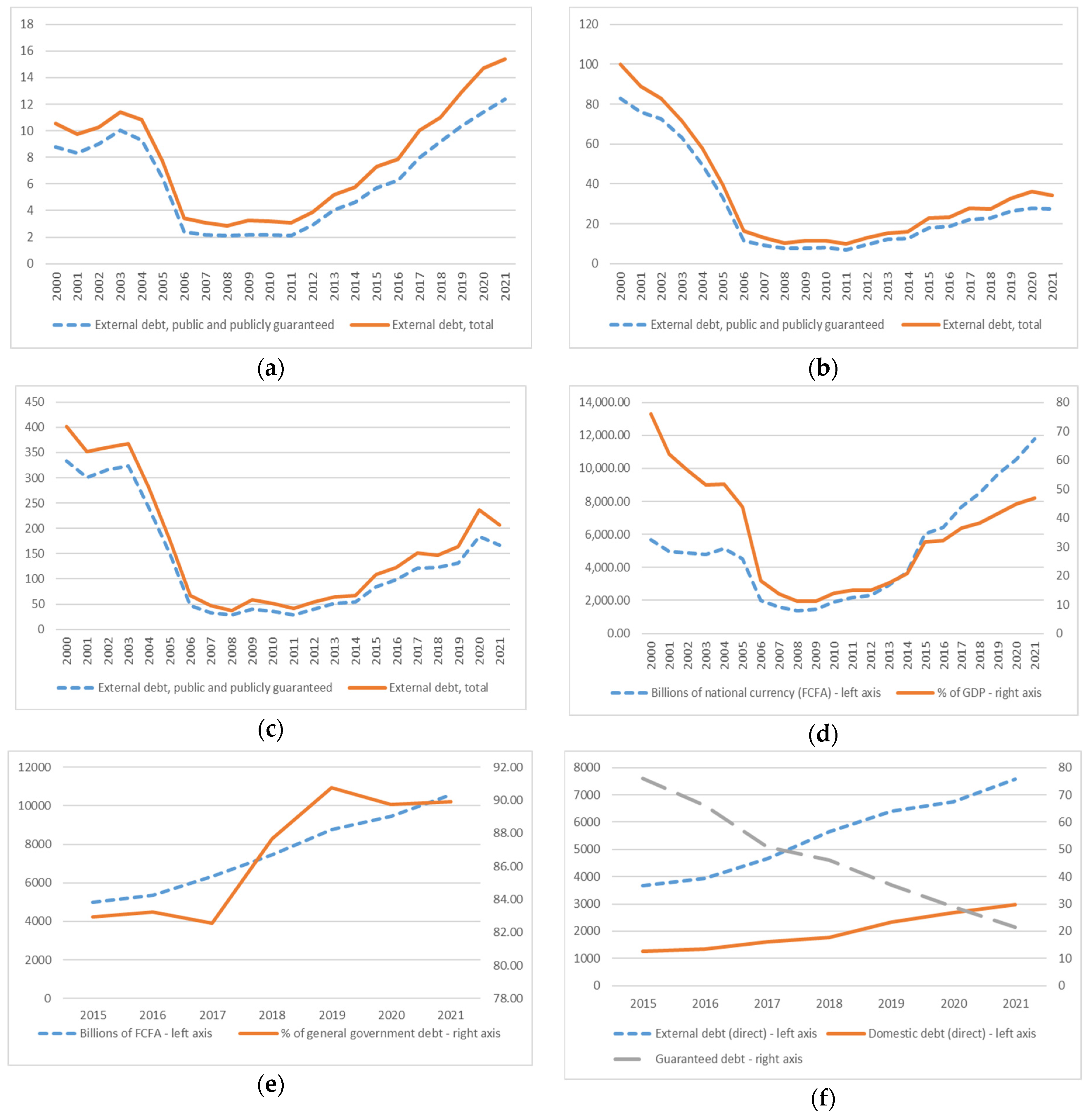
Disclaimer/Publisher’s Note: The statements, opinions and data contained in all publications are solely those of the individual author(s) and contributor(s) and not of MDPI and/or the editor(s). MDPI and/or the editor(s) disclaim responsibility for any injury to people or property resulting from any ideas, methods, instructions or products referred to in the content. |
© 2024 by the authors. Licensee MDPI, Basel, Switzerland. This article is an open access article distributed under the terms and conditions of the Creative Commons Attribution (CC BY) license (https://creativecommons.org/licenses/by/4.0/).