
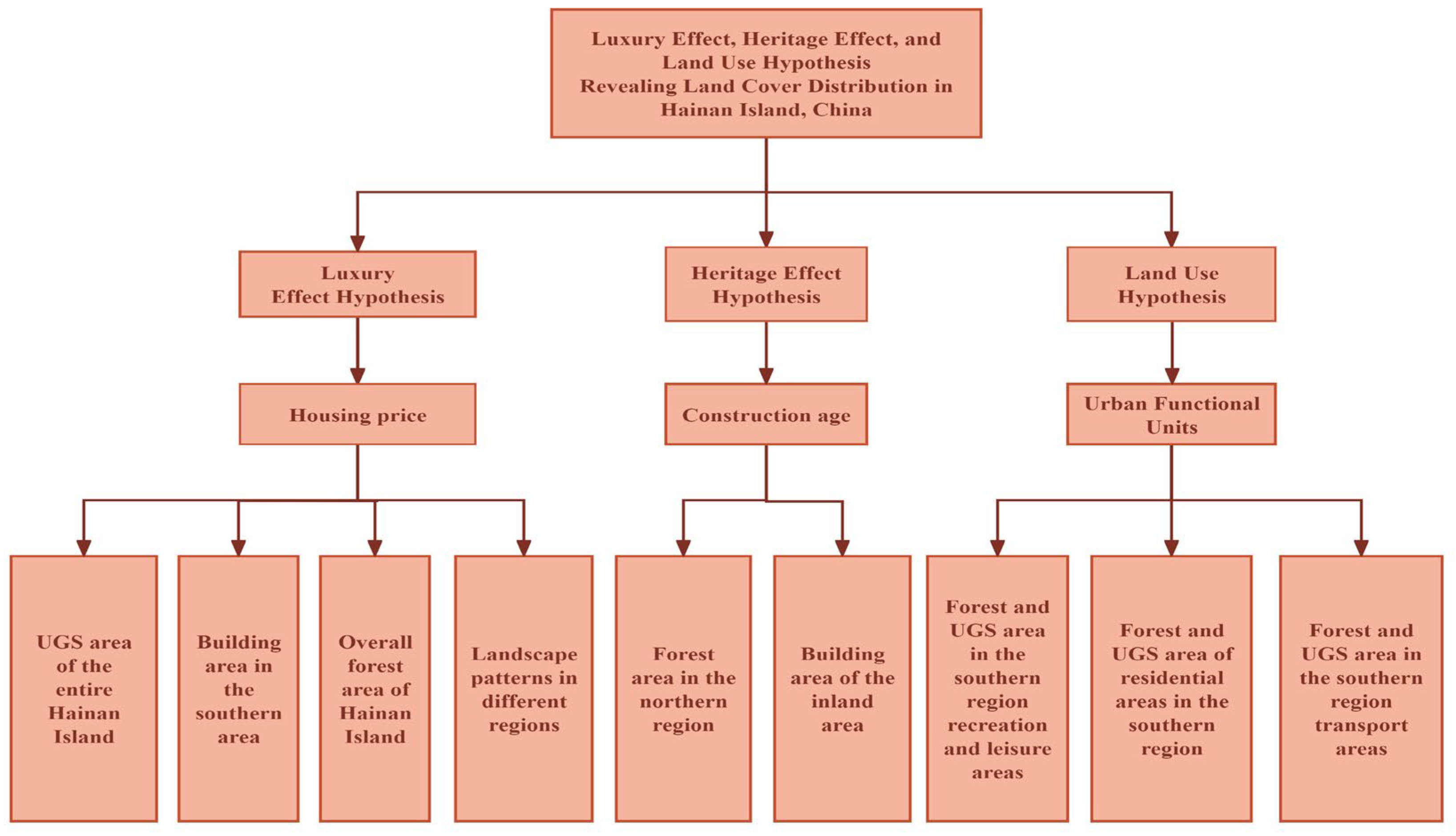
Luxury Effect, Heritage Effect, and Land Use Hypotheses Revealing Land Cover Distribution in Hainan Island, China


 ,
, 
Abstract
:1. Introduction
2. Materials and Methods
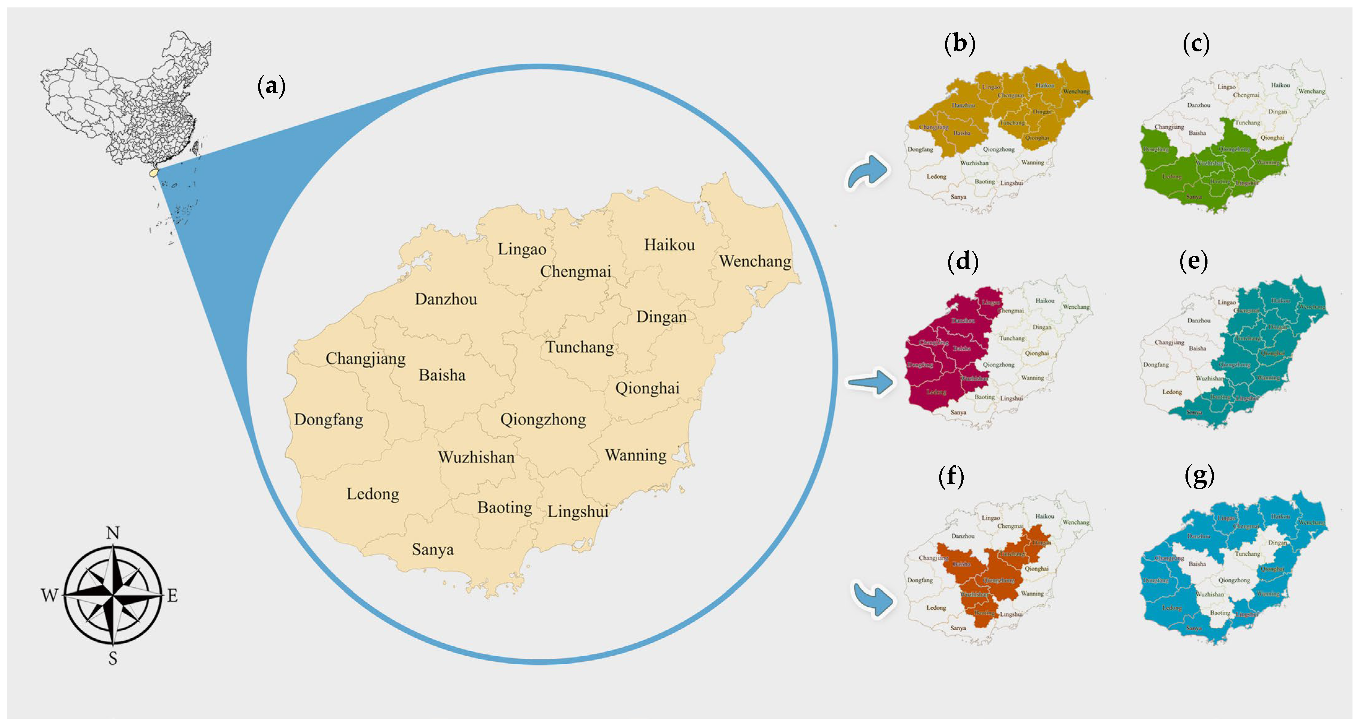
2.1. Study Area
2.2. Sampling Design of Urban Functional Units (UFUs)
2.3. LC Data and Landscape Indicators
2.4. Factors of Social and Economic Variables
2.5. Statistical Analysis
3. Results
3.1. Driving Factors Affecting LC Distribution in the South and North of Hainan Island
3.2. Driving Factors Affecting LC Distribution in the East and West of Hainan Island
3.3. Driving Factors Affecting the LC Distribution in the Inland and Coastal Areas of Hainan Island
3.4. Driving Factors Affecting the LC Distribution of Hainan Island as a Whole and of 18 Counties and Cities
4. Discussion
4.1. Luxury Effect Test of the Mechanism Driving LC Changes
4.2. Heritage Effect Test of the Mechanism That Drives LC Change
4.3. The Land Use Hypothesis Tests the Mechanism Driving the LC Change of UFUs
4.4. Study Limitations
5. Conclusions
Supplementary Materials
Author Contributions
Funding
Institutional Review Board Statement
Informed Consent Statement
Data Availability Statement
Acknowledgments
Conflicts of Interest
References
- Gemitzi, A.; Banti, M.A.; Lakshmi, V. Vegetation greening trends in different land use types: Natural variability versus human-induced impacts in Greece. Environ. Earth Sci. 2019, 78, 172. [Google Scholar] [CrossRef]
- Ojima, D.; Galvin, K.; Turner Ii, B.L. The Global Impact of Land-Use Change. Bioscience 1994, 44, 300–304. [Google Scholar] [CrossRef]
- Zhao, Q.; Wen, Z.; Chen, S.; Ding, S.; Zhang, M. Quantifying Land Use/Land Cover and Landscape Pattern Changes and Impacts on Ecosystem Services. Int. J. Environ. Res. Public Health 2020, 17, 126. [Google Scholar]
- Ellis, E.C.; Beusen, A.H.; Klein Goldewijk, K. Anthropogenic biomes: 10,000 BCE to 2015 CE. Land 2020, 9, 129. [Google Scholar] [CrossRef]
- Liu, H.; Gong, P.; Wang, J.; Clinton, N.; Bai, Y.; Liang, S. Annual dynamics of global land cover and its long-term changes from 1982 to 2015. Earth Syst. Sci. Data 2020, 12, 1217–1243. [Google Scholar]
- Nguyen, H.M.; Nguyen, L.D. The relationship between urbanization and economic growth: An empirical study on ASEAN countries. Int. J. Soc. Econ. 2018, 45, 316–339. [Google Scholar]
- Cohen, B. Urbanization in developing countries: Current trends, future projections, and key challenges for sustainability. Technol. Soc. 2006, 28, 63–80. [Google Scholar]
- Turok, I.; McGranahan, G. Urbanization and economic growth: The arguments and evidence for Africa and Asia. Environ. Urban. 2013, 25, 465–482. [Google Scholar]
- Rao, Y.; Zhong, Y.; He, Q.; Dai, J. Assessing the equity of accessibility to urban green space: A study of 254 cities in China. Int. J. Environ. Res. Public Health 2022, 19, 4855. [Google Scholar] [CrossRef]
- Wang, Y.; Yang, X. Fiscal ecological cost of land in China: Estimation and regional differences. Land 2022, 11, 1221. [Google Scholar] [CrossRef]
- Wiatkowska, B.; Słodczyk, J.; Stokowska, A. Spatial-temporal land use and land cover changes in urban areas using remote sensing images and GIS analysis: The case study of Opole, Poland. Geosciences 2021, 11, 312. [Google Scholar] [CrossRef]
- Schell, C.J.; Dyson, K.; Fuentes, T.L.; Des Roches, S.; Harris, N.C.; Miller, D.S.; Woelfle-Erskine, C.A.; Lambert, M.R. The ecological and evolutionary consequences of systemic racism in urban environments. Science 2020, 369, eaay4497. [Google Scholar]
- Grove, J.M.; Locke, D.H.; O’Neil-Dunne, J.P. An ecology of prestige in New York City: Examining the relationships among population density, socio-economic status, group identity, and residential canopy cover. Environ. Manag. 2014, 54, 402–419. [Google Scholar]
- Locke, D.H.; Hall, B.; Grove, J.M.; Pickett, S.T.; Ogden, L.A.; Aoki, C.; Boone, C.G.; O’Neil-Dunne, J.P. Residential housing segregation and urban tree canopy in 37 US Cities. npj Urban Sustain. 2021, 1, 15. [Google Scholar]
- Hope, D.; Gries, C.; Zhu, W.; Fagan, W.F.; Redman, C.L.; Grimm, N.B.; Nelson, A.L.; Martin, C.; Kinzig, A. Socioeconomics drive urban plant diversity. Proc. Natl. Acad. Sci. USA 2003, 100, 8788–8792. [Google Scholar]
- Blicharska, M.; Andersson, J.; Bergsten, J.; Bjelke, U.; Hilding-Rydevik, T.; Thomsson, M.; Östh, J.; Johansson, F. Is there a relationship between socio-economic factors and biodiversity in urban ponds? A study in the city of Stockholm. Urban Ecosyst. 2017, 20, 1209–1220. [Google Scholar]
- Zhang, H.-L.; Cubino, J.P.; Nizamani, M.M.; Harris, A.; Cheng, X.-L.; Da, L.; Sun, Z.; Wang, H.-F. Wealth and land use drive the distribution of urban green space in the tropical coastal city of Haikou, China. Urban For. Urban Green. 2022, 71, 127554. [Google Scholar]
- Baró, F.; Calderón-Argelich, A.; Langemeyer, J.; Connolly, J.J. Under one canopy? Assessing the distributional environmental justice implications of street tree benefits in Barcelona. Environ. Sci. Policy 2019, 102, 54–64. [Google Scholar]
- Clarke, L.W.; Jenerette, G.D.; Davila, A. The luxury of vegetation and the legacy of tree biodiversity in Los Angeles, CA. Landsc. Urban Plan. 2013, 116, 48–59. [Google Scholar]
- Boone, C.G.; Cadenasso, M.L.; Grove, J.M.; Schwarz, K.; Buckley, G.L. Landscape, vegetation characteristics, and group identity in an urban and suburban watershed: Why the 60s matter. Urban Ecosyst. 2010, 13, 255–271. [Google Scholar]
- Celińska-Janowicz, D.; Smętkowski, M.; Wojnar, K. Behavioural Aspects of Office Space Structures in the City: The Case of Warsaw’s Business Districts. Urban Plan. 2021, 6, 431–443. [Google Scholar]
- Sevtsuk, A. Path and Place: A Study of Urban Geometry and Retail Activity in Cambridge and Somerville, MA; Massachusetts Institute of Technology: Cambridge, MA, USA, 2010. [Google Scholar]
- Lau, S.S.Y.; Giridharan, R.; Ganesan, S. Multiple and intensive land use: Case studies in Hong Kong. Habitat Int. 2005, 29, 527–546. [Google Scholar]
- Yan, J.; Zhou, W.; Zheng, Z.; Wang, J.; Tian, Y. Characterizing variations of greenspace landscapes in relation to neighborhood characteristics in urban residential area of Beijing, China. Landsc. Ecol. 2020, 35, 203–222. [Google Scholar]
- Azarnert, L.V. Migration, congestion, and growth. Macroecon. Dyn. 2019, 23, 3035–3064. [Google Scholar]
- Azarnert, L.V. Population sorting and human capital accumulation. Oxf. Econ. Pap. 2023, 75, 780–801. [Google Scholar]
- Li, H.; Peng, J.; Yanxu, L.; Yi’na, H. Urbanization impact on landscape patterns in Beijing City, China: A spatial heterogeneity perspective. Ecol. Indic. 2017, 82, 50–60. [Google Scholar]
- Cheng, X.L.; Nizamani, M.M.; Jim, C.Y.; Balfour, K.; Da, L.J.; Qureshi, S.; Zhu, Z.X.; Wang, H.F. Using SPOT Data and FRAGSTAS to analyze the relationship between plant diversity and green space landscape patterns in the tropical coastal city of Zhanjiang, China. Remote Sens. 2020, 12, 3477. [Google Scholar] [CrossRef]
- Zou, L.; Wang, J.; Bai, M. Assessing spatial–temporal heterogeneity of China’s landscape fragmentation in 1980–2020. Ecol. Indic. 2022, 136, 108654. [Google Scholar] [CrossRef]
- Fischer, J.; Lindenmayer, D.B. Landscape modification and habitat fragmentation: A synthesis. Glob. Ecol. Biogeogr. 2007, 16, 265–280. [Google Scholar]
- Tang, Z.; Wang, Y.; Fu, M.; Xue, J. The role of land use landscape patterns in the carbon emission reduction: Empirical evidence from China. Ecol. Indic. 2023, 156, 111176. [Google Scholar]
- Jia, Y.; Tang, L.; Xu, M.; Yang, X. Landscape pattern indices for evaluating urban spatial morphology—A case study of Chinese cities. Ecol. Indic. 2019, 99, 27–37. [Google Scholar]
- Wang, Q.; Wang, H. Spatiotemporal dynamics and evolution relationships between land-use/land cover change and landscape pattern in response to rapid urban sprawl process: A case study in Wuhan, China. Ecol. Eng. 2022, 182, 106716. [Google Scholar]
- Motlagh, Z.K.; Lotfi, A.; Pourmanafi, S.; Ahmadizadeh, S.; Soffianian, A. Spatial modeling of land-use change in a rapidly urbanizing landscape in central Iran: Integration of remote sensing, CA-Markov, and landscape metrics. Environ. Monit. Assess. 2020, 192, 1–19. [Google Scholar]
- Weng, H.; Gao, Y.; Su, X.; Yang, X.; Cheng, F.; Ma, R.; Liu, Y.; Zhang, W.; Zheng, L. Spatial-temporal changes and driving force analysis of green space in coastal cities of Southeast China over the past 20 years. Land 2021, 10, 537. [Google Scholar] [CrossRef]
- Chen, W.; Zeng, J.; Li, N. Change in land-use structure due to urbanisation in China. J. Clean. Prod. 2021, 321, 128986. [Google Scholar]
- Zhang, Y.; Qin, K.; Bi, Q.; Cui, W.; Li, G. Landscape patterns and building functions for urban land-use classification from remote sensing images at the block level: A case study of Wuchang District, Wuhan, China. Remote Sens. 2020, 12, 1831. [Google Scholar] [CrossRef]
- Zhu, M.; Cubino, J.P.; Johnson, J.B.; Cui, J.; Khokhar, A.A.; Guo, L.-Y.; Hughes, A.C.; Wang, H.-F. The legacy effect and urban management planning driving changes in Urban Green Spaces land use in Haikou city, Hainan province: A comprehensive analysis. Trop. Plants 2024, 3, e011. [Google Scholar]
- Wang, H.-F.; Cheng, X.-L.; Nizamani, M.M.; Balfour, K.; Da, L.; Zhu, Z.-X.; Qureshi, S. An Integrated approach to study spatial patterns and drivers of land cover within urban functional units: A multi-city comparative study in China. Remote Sens. 2020, 12, 2201. [Google Scholar] [CrossRef]
- Zhai, H.; Lv, C.; Liu, W.; Yang, C.; Fan, D.; Wang, Z.; Guan, Q. Understanding spatio-temporal patterns of land use/land cover change under urbanization in Wuhan, China, 2000–2019. Remote Sens. 2021, 13, 3331. [Google Scholar] [CrossRef]
- Naikoo, M.W.; Islam, A.R.M.T.; Mallick, J.; Rahman, A. Land use/land cover change and its impact on surface urban heat island and urban thermal comfort in a metropolitan city. Urban Clim. 2022, 41, 101052. [Google Scholar]
- Alshari, E.A.; Gawali, B.W. Development of classification system for LULC using remote sensing and GIS. Glob. Transit. Proc. 2021, 2, 8–17. [Google Scholar]
- Gu, Z.; Zeng, M. The use of artificial intelligence and satellite remote sensing in land cover change detection: Review and perspectives. Sustainability 2023, 16, 274. [Google Scholar] [CrossRef]
- Radwan, T.M.; Blackburn, G.A.; Whyatt, J.D.; Atkinson, P.M. Global land cover trajectories and transitions. Sci. Rep. 2021, 11, 12814. [Google Scholar]
- Jing, Q.; He, J.; Li, Y.; Yang, X.; Peng, Y.; Wang, H.; Yu, F.; Wu, J.; Gong, S.; Che, H. Analysis of the spatiotemporal changes in global land cover from 2001 to 2020. Sci. Total Environ. 2024, 908, 168354. [Google Scholar] [PubMed]
- Gong, D.; Huang, M.; Lin, H. Construction of an Ecological Security Pattern in Rapidly Urbanizing Areas Based on Ecosystem Sustainability, Stability, and Integrity. Remote Sens. 2023, 15, 5728. [Google Scholar] [CrossRef]
- Zhang, H.L.; Guo, L.Y.; Nizamani, M.M.; Wang, H.F. Distribution patterns and drivers of urban green space and plant diversity in Haikou, China. Front. Plant Sci. 2023, 14, 1202115. [Google Scholar] [CrossRef]
- Cui, J.P.; Zhu, M.H.; Guo, L.Y.; Zhang, H.L.; Hughes, A.C.; Wang, H.F. Urban Planning and Green Landscape Management Drive Plant Diversity in Five Tropical Cities in China. Sustainability 2023, 15, 12045. [Google Scholar] [CrossRef]
- Sapena, M.; Ruiz, L.A.; Taubenböck, H. Analyzing links between spatio-temporal metrics of built-up areas and socio-economic indicators on a semi-global scale. ISPRS Int. J. Geo-Inf. 2020, 9, 436. [Google Scholar] [CrossRef]
- Tessema, M.W.; Abebe, B.G.; Bantider, A. Physical and socioeconomic driving forces of land use and land cover changes: The case of Hawassa City, Ethiopia. Front. Environ. Sci. 2024, 12, 1203529. [Google Scholar]
- Najafi, E.; Hosseinali, F.; Najafi, M.M.; Sharifi, A. A GIS-based Evaluation of Urban Livability using Factor Analysis and a Combination of Environmental and Socio-economic Indicators. J. Geovisualization Spat. Anal. 2024, 8, 27. [Google Scholar]
- Toure, S.I.; Stow, D.A.; Clarke, K.; Weeks, J. Patterns of land cover and land use change within the two major metropolitan areas of Ghana. Geocarto Int. 2020, 35, 209–223. [Google Scholar]
- Hu, J.; Wang, Y.; Taubenböck, H.; Zhu, X.X. Land consumption in cities: A comparative study across the globe. Cities 2021, 113, 103163. [Google Scholar]
- Wu, Y.; Li, S.; Yu, S. Monitoring urban expansion and its effects on land use and land cover changes in Guangzhou city, China. Environ. Monit. Assess. 2016, 188, 54. [Google Scholar] [PubMed]
- Dadashpoor, H.; Azizi, P.; Moghadasi, M. Land use change, urbanization, and change in landscape pattern in a metropolitan area. Sci. Total Environ. 2019, 655, 707–719. [Google Scholar]
- Asabere, S.B.; Acheampong, R.A.; Ashiagbor, G.; Beckers, S.C.; Keck, M.; Erasmi, S.; Schanze, J.; Sauer, D. Urbanization, land use transformation and spatio-environmental impacts: Analyses of trends and implications in major metropolitan regions of Ghana. Land Use Policy 2020, 96, 104707. [Google Scholar]
- Zhang, H.; Qi, Z.-f.; Ye, X.-y.; Cai, Y.-b.; Ma, W.-c.; Chen, M.-n. Analysis of land use/land cover change, population shift, and their effects on spatiotemporal patterns of urban heat islands in metropolitan Shanghai, China. Appl. Geogr. 2013, 44, 121–133. [Google Scholar]
- Montgomery, M.R. The Urban Transformation of the Developing World. Science 2008, 319, 761–764. [Google Scholar] [CrossRef]
- Desa, U. World Urbanization Prospects: The 2014 Revision; United Nations Department of Economics and Social Affairs. Population Division: New York, NY, USA, 2015; Volume 41. [Google Scholar]
- Zhang, C.; Sun, Z.; Xing, Q.; Sun, J.; Xia, T.; Yu, H. Localizing Indicators of SDG11 for an Integrated Assessment of Urban Sustainability—A Case Study of Hainan Province. Sustainability 2021, 13, 11092. [Google Scholar] [CrossRef]
- Liang, A.; Yan, D.; Yan, J.; Lu, Y.; Wang, X.; Wu, W. A Comprehensive Assessment of Sustainable Development of Urbanization in Hainan Island Using Remote Sensing Products and Statistical Data. Sustainability 2023, 15, 979. [Google Scholar] [CrossRef]
- Hei, N. A List of Specific Regional Divisions in Hainan. Available online: https://haikou.bendibao.com/news/2024116/64609.shtm (accessed on 16 January 2016).
- Usman, K. China’s Special Economic Zones, Hainan Province New Free Trade Zone: Review of Policies that Minimize the Regional Gap. J. Manag. Econ. Stud. 2020, 2, 99–111. [Google Scholar]
- Fu, J.; Zhang, Q.; Wang, P.; Zhang, L.; Tian, Y.; Li, X. Spatio-temporal changes in ecosystem service value and its coordinated development with economy: A case study in Hainan Province, China. Remote Sens. 2022, 14, 970. [Google Scholar] [CrossRef]
- Department of Population (Social Sciences), Hainan Provincial Bureau of Statistics. In 2023, the Permanent Resident Population of the Province Will Increase Steadily. Available online: https://stats.hainan.gov.cn/tjj/ywdt/xwfb/202404/t20240401_3634981.html (accessed on 1 April 2024).
- Hainan Daily. In 2023, the Province’s GDP Reached 755.118 Billion Yuan, an Increase of 9.2%. Available online: https://www.hainan.gov.cn/hainan/c100690/202401/69c3e3a0fa7a4fbcb34dd3a7ec3efdce.shtml?ddtab=true (accessed on 20 January 2024).
- Yang, X. 2023 GDP Data for China’s|31 Provinces Are Released. Available online: http://finance.people.com.cn/n1/2024/0131/c1004-40170326.html (accessed on 31 January 2024).
- Guo, L.-Y.; Nizamani, M.M.; Harris, A.J.; Padullés Cubino, J.; Johnson, J.B.; Cui, J.-P.; Zhang, H.-L.; Zhou, J.-J.; Zhu, Z.-X.; Wang, H.-F. Anthropogenic factors explain urban plant diversity across three tropical cities in China. Urban For. Urban Green. 2024, 95, 128323. [Google Scholar] [CrossRef]
- Nowak, D.J.; Crane, D.E.; Stevens, J.C.; Hoehn, R.E. The Urban Forest Effects (UFORE) Model: Field Data Collection Manual; US Department of Agriculture Forest Service, Northeastern Research Station: Syracuse, NY, USA, 2003; pp. 4–11. [Google Scholar]
- Zhang, H.-L.; Nizamani, M.M.; Guo, L.-Y.; Cui, J.; Padullés Cubino, J.; Hughes, A.C.; Wang, H.-F. Interplay of socio-economic and environmental factors in shaping urban plant biodiversity: A comprehensive analysis. Front. Ecol. Evol. 2024, 12, 1344343. [Google Scholar]
- Sun, L.; Chen, J.; Li, Q.; Huang, D. Dramatic uneven urbanization of large cities throughout the world in recent decades. Nat. Commun. 2020, 11, 5366. [Google Scholar] [PubMed]
- Chu, M.; Pan, L.; Guo, M.; Xu, L.; Zong, J. Has high housing prices affected urban green development?: Evidence from China. J. Hous. Built Environ. 2023, 38, 2185–2206. [Google Scholar]
- Hu, W.; Yin, S.; Gong, H. Spatial–Temporal Evolution Patterns and Influencing Factors of China’s Urban Housing Price-to-Income Ratio. Land 2022, 11, 2224. [Google Scholar] [CrossRef]
- Berry, B.J. Urbanization. In Urban Ecology: An International Perspective on the Interaction between Humans Nature; Springer: Berlin/Heidelberg, Germany, 2008; pp. 25–48. [Google Scholar]
- van der Woude, A.M.; Hayami, A.; De Vries, J. Urbanization in History: A Process of Dynamic Interactions; Oxford University Press: Oxford, UK, 1990. [Google Scholar]
- Santos, M.J.; Smith, A.B.; Dekker, S.C.; Eppinga, M.B.; Leitão, P.J.; Moreno-Mateos, D.; Morueta-Holme, N.; Ruggeri, M. The role of land use and land cover change in climate change vulnerability assessments of biodiversity: A systematic review. Landsc. Ecol. 2021, 36, 3367–3382. [Google Scholar]
- Meyer, W.B.; Turner, B.L. Human population growth and global land-use/cover change. Annu. Rev. Ecol. Syst. 1992, 23, 39–61. [Google Scholar]
- Wang, H.F.; Qureshi, S.; Qureshi, B.A.; Qiu, J.X.; Friedman, C.R.; Breuste, J.; Wang, X.K. A multivariate analysis integrating ecological, socioeconomic and physical characteristics to investigate urban forest cover and plant diversity in Beijing, China. Ecol. Indic. 2016, 60, 921–929. [Google Scholar] [CrossRef]
- Zill, D.G. Advanced Engineering Mathematics; Jones & Bartlett Learning: Burlington, MA, USA, 2020. [Google Scholar]
- Kreyszig, E. Advanced Engineering Mathematics; John Wiley: New York, NY, USA, 1975; pp. 707–709+783–787. [Google Scholar]
- Lynch, L.; Kangas, M.; Ballut, N.; Doucet, A.; Schoenecker, K.; Johnson, P.; Gharehaghaji, M.; Minor, E.S. Changes in land use and land cover along an urban-rural gradient influence floral resource availability. Curr. Landsc. Ecol. Rep. 2021, 6, 46–70. [Google Scholar]
- Buyantuyev, A.; Wu, J. Urban heat islands and landscape heterogeneity: Linking spatiotemporal variations in surface temperatures to land-cover and socioeconomic patterns. Landsc. Ecol. 2010, 25, 17–33. [Google Scholar]
- Sudmeier-Rieux, K.; Paleo, U.F.; Garschagen, M.; Estrella, M.; Renaud, F.G.; Jaboyedoff, M. Opportunities, incentives and challenges to risk sensitive land use planning: Lessons from Nepal, Spain and Vietnam. Int. J. Disaster Risk Reduct. 2015, 14, 205–224. [Google Scholar]
- Sirgy, M.J. Materialism and quality of life. Soc. Indic. Res. 1998, 43, 227–260. [Google Scholar]
- Palliwoda, J.; Priess, J.A. What do people value in urban green? Linking characteristics of urban green spaces to users’ perceptions of nature benefits, disturbances, and disservices. Ecol. Soc. 2021, 26, 28. [Google Scholar]
- Zalejska-Jonsson, A.; Wilkinson, S.J.; Wahlund, R. Willingness to pay for green infrastructure in residential development—A consumer perspective. Atmosphere 2020, 11, 152. [Google Scholar] [CrossRef]
- Pan, R. The “Hainan” Lesson in China’s Real Estate Industry—The Overheated Hainan Housing Market in the Early 1990s and Its Influence; University of Reading: Reading, UK, 2020. [Google Scholar]
- Aznarez, C.; Svenning, J.C.; Pacheco, J.P.; Have Kallesøe, F.; Baró, F.; Pascual, U. Luxury and legacy effects on urban biodiversity, vegetation cover and ecosystem services. Urban Sustain. 2023, 3, 47. [Google Scholar]
- Creamer, C.A.; Filley, T.R.; Boutton, T.W.; Rowe, H.I. Grassland to woodland transitions: Dynamic response of microbial community structure and carbon use patterns. J. Geophys. Res. Biogeosci. 2016, 121, 1675–1688. [Google Scholar]
- Siemann, E.; Rogers, W.E. Changes in light and nitrogen availability under pioneer trees may indirectly facilitate tree invasions of grasslands. J. Ecol. 2003, 91, 923–931. [Google Scholar]
- Adie, H.; Lawes, M.J. Solutions to fire and shade: Resprouting, growing tall and the origin of Eurasian temperate broadleaved forest. Biol. Rev. 2023, 98, 643–661. [Google Scholar]
- Gao, X.; Li, C.; Cai, Y.; Ye, L.; Xiao, L.; Zhou, G.; Zhou, Y. Influence of Scale Effect of Canopy Projection on Understory Microclimate in Three Subtropical Urban Broad-Leaved Forests. Remote Sens. 2021, 13, 3786. [Google Scholar] [CrossRef]
- Misiune, I.; Kazys, J. Accessibility to and Fragmentation of Urban Green Infrastructure: Importance for Adaptation to Climate Change. In Ieva Misiune Daniel Depellegrin; Springer: Berlin/Heidelberg, Germany, 2022; p. 235. [Google Scholar]
- Jim, C.Y.; Chen, S.S. Comprehensive greenspace planning based on landscape ecology principles in compact Nanjing city, China. Landsc. Urban Plan. 2003, 65, 95–116. [Google Scholar]
- Cacabelos, E.; Neto, A.I.; Martins, G.M. Gastropods with different development modes respond differently to habitat fragmentation. Mar. Environ. Res. 2021, 167, 105287. [Google Scholar] [PubMed]
- Kheir, A.-K. High-Rise Developments: A Critical Review of the Nature and Extent of Their Sustainability. In Pragmatic Engineering Lifestyle: Responsible Engineering for a Sustainable Future; Emerald Publishing Limited: Leeds, UK, 2023; pp. 1–20. [Google Scholar]
- Permanasari, E.; Hendola, F.; Tarigan, S.; Tafridj, I.; Aurora, F. Urban expansion in South Tangerang: Analyzing Bintaro Jaya as a private city. Cities 2024, 144, 104665. [Google Scholar]
- Vidal, D.G.; Barros, N.; Maia, R.L. Public and green spaces in the context of sustainable development. In Sustainable Cities and Communities; Springer: Berlin/Heidelberg, Germany, 2020; pp. 479–487. [Google Scholar]
- Ahn, Y.-J.; Juraev, Z. Green spaces in Uzbekistan: Historical heritage and challenges for urban environment. Nat.-Based Solut. 2023, 4, 100077. [Google Scholar]
- Huang, J.; Tang, Z.; Liu, D.; He, J. Ecological response to urban development in a changing socio-economic and climate context: Policy implications for balancing regional development and habitat conservation. Land Use Policy 2020, 97, 104772. [Google Scholar]
- Swetnam, T.W.; Allen, C.D.; Betancourt, J.L. Applied historical ecology: Using the past to manage for the future. Ecol. Appl. 1999, 9, 1189–1206. [Google Scholar]
- Zhang, Y.; Uusivuori, J.; Kuuluvainen, J. Econometric analysis of the causes of forest land use changes in Hainan, China. Can. J. For. Res. 2000, 30, 1913–1921. [Google Scholar]
- Bao, K. The provincial government is making an initiation: Experiment of sustainable development in hainan. In Proceedings of the International Advisory Meeting on the Economic Development of Hainan in Harmony with the Natural Environment, Haikou, China, September 1990; pp. 13–14. [Google Scholar]
- Tang, Y.; Wei, Z.C.; Wang, P. Spatial temporal differences of regional balance degree on land use based on GIS: A case study in Hainan Province. Chin. J. Agric. Resour. Reg. Plan. 2017, 38, 41–47. [Google Scholar]
- Long, H.; Li, Y.; Liu, Y.; Woods, M.; Zou, J. Accelerated restructuring in rural China fueled by ‘increasing vs. decreasing balance’land-use policy for dealing with hollowed villages. Land Use Policy 2012, 29, 11–22. [Google Scholar]
- The People’s Government of Hainan Province. Notice of the General Office of the People’s Government of Hainan Province on Issuing Opinions on Several Issues Concerning the Disposal of State-Owned Construction Land Stock in Hainan Province (2016) No. 241. Available online: https://www.hainan.gov.cn/hainan/szfbgtwj/201610/a2107f136f86477fa6dd3b6ee88fbed7.shtml (accessed on 9 October 2016).
- Yuan, Y. The “Several Provisions on the Disposal of Idle Land in Hainan Free Trade Port” Promotes the Solution to the Problem of Idle and Inefficient Land Disposal. Available online: https://www.hainan.gov.cn/hainan/yqfkzzzzxxxng/202206/951e67c9765b49fbb1e2fac7ad6376a0.shtml (accessed on 9 June 2022).
- Li, T.; Zhang, S.; Cao, X.; Witlox, F. Does a circular high-speed rail network promote efficiency and spatial equity in transport accessibility? Evidence from Hainan Island, China. Transp. Plan. Technol. 2018, 41, 779–795. [Google Scholar]
- Yang, G.; Yang, K.; Zhu, F.; Mao, Y.; Mao, Y.; Zeng, Z.; Dong, X. Hainan of China: The evolution from a special economic zone to a comprehensive and compound free trade port. Geogr. Res. 2018, 37, 2363–2382. [Google Scholar] [CrossRef]
- Fang, X.; Liu, W. Exploring Intra-Island Population Mobility and Economic Resilience: The Case of Hainan Island, China. Sustainability 2023, 15, 16772. [Google Scholar] [CrossRef]
- Xiu, C.; Li, T. Construction of the Hainan Free Trade Port from the perspective of regional cultural development. Front. Earth Sci. 2023, 10, 1032953. [Google Scholar]
- Weber, R. Extracting value from the city: Neoliberalism and urban redevelopment. Antipode 2002, 34, 519–540. [Google Scholar]
- The People’s Government of Hainan Province. Notice of the General Office of the People’s Government of Hainan Province on the Issuance of the Implementation Plan for Accelerating the Development of the Central Region in 2003, Qiongfu Office (2003) No. 33. Available online: https://www.hainan.gov.cn/data/zfgb/2019/10/7679/ (accessed on 15 June 2003).
- Yang, G. Development of central China and construction of Hainan ecological province. J. Qiongzhou Univ. 2000, 7, 52–53. [Google Scholar]
- Liu, C.; Zhang, H.; LI, Q. Spatiotemporal characteristics of human activity intensity and its driving mechanism in Hainan Island from 1980 to 2018. Prog. Geogr. 2020, 39, 10. [Google Scholar] [CrossRef]
- Chen, H.; Li, D.; Chen, Y.; Zhao, Z. Spatial–Temporal Evolution Monitoring and Ecological Risk Assessment of Coastal Wetlands on Hainan Island, China. Remote Sens. 2023, 15, 1035. [Google Scholar] [CrossRef]
- Wang, D.; Pei, L.-x.; Zhang, L.-z.; Li, X.-w.; Chen, Z.-h.; Zhou, Y.-h. Research Paper Water resource utilization characteristics and driving factors in the Hainan Island. J. Groundw. Sci. Eng. 2017, 5, 354–363. [Google Scholar]
- Li, L.; Tang, H.; Lei, J.; Song, X. Spatial autocorrelation in land use type and ecosystem service value in Hainan Tropical Rain Forest National Park. Ecol. Indic. 2022, 137, 108727. [Google Scholar]
- Pozoukidou, G.; Chatziyiannaki, Z. 15-Minute City: Decomposing the new urban planning eutopia. Sustainability 2021, 13, 928. [Google Scholar] [CrossRef]
- Bonu, M.S.; Verboom, J.; Schultner, J. Urban Green Space Maintenance and Multiple Ecosystem Services: A Case Study of Parks in Wageningen Inner City. Master’s Thesis, Wageningen University and Research, Wageningen, The Netherlands, 2023. [Google Scholar]
- Marques da Costa, E.; Kállay, T. Impacts Of Green Spaces on Physical and Mental Health; EU, URBACT: Paris, France, 2020. [Google Scholar]
- Abuseif, M.; Dupre, K.; Michael, R.N. Trees on buildings: Opportunities, challenges, and recommendations. Build. Environ. 2022, 225, 109628. [Google Scholar]
- Sanusi, R.; Johnstone, D.; May, P.; Livesley, S.J. Street orientation and side of the street greatly influence the microclimatic benefits street trees can provide in summer. J. Environ. Qual. 2016, 45, 167–174. [Google Scholar]
- Armson, D.; Stringer, P.; Ennos, A.R. The effect of tree shade and grass on surface and globe temperatures in an urban area. Urban For. Urban Green. 2012, 11, 245–255. [Google Scholar]
- Shams, I.; Barker, A. Barriers and opportunities of combining social and ecological functions of urban greenspaces–Users’ and landscape professionals’ perspectives. Urban For. Urban Green. 2019, 39, 67–78. [Google Scholar]
- Hansen, G.; Macedo, J. Urban Ecology for Citizens and Planners; University Press of Florida: Gainesville, FL, USA, 2021. [Google Scholar]
- Pantaloni, M.; Marinelli, G.; Santilocchi, R.; Minelli, A.; Neri, D. Sustainable Management Practices for Urban Green Spaces to Support Green Infrastructure: An Italian Case Study. Sustainability 2022, 14, 4243. [Google Scholar] [CrossRef]
- Mao, Y.; Zhou, X.W. Land fill Hainan policy consummation under the construction of ecological civilization view. J. Heilongjiang Vocat. Inst. Ecol. Eng. 2017, 30, 7–9. [Google Scholar]
- Wang, Y.; Wang, T.; Fu, S. Discussion on the status quo and management countermeasures of land reclamation in Hainan Province. Ocean Dev. Manag. 2015, 32, 56–59. [Google Scholar]
- Wang, W.; Liu, H.; Li, Y.; Su, J. Development and management of land reclamation in China. Ocean Coast. Manag. 2014, 102, 415–425. [Google Scholar]
- Breuste, J.; Artmann, M.; Faggi, A.; Breuste, J.; Breuste, J.; Zippel, S.; Gimenez-Maranges, M.; Hayir-Kanat, M.; Breuste, J.; Hansen, R.; et al. Multi-functional urban green spaces. In Making Green Cities: Concepts, Challenges and Practice; Springer: Berlin/Heidelberg, Germany, 2020; pp. 399–526. [Google Scholar]
- Yamanaka, S.; Ishiyama, N.; Senzaki, M.; Morimoto, J.; Kitazawa, M.; Fuke, N.; Nakamura, F. Role of flood-control basins as summer habitat for wetland species-a multiple-taxon approach. Ecol. Eng. 2020, 142, 105617. [Google Scholar]
- Alikhani, S.; Nummi, P.; Ojala, A. Urban wetlands: A review on ecological and cultural values. Water 2021, 13, 3301. [Google Scholar] [CrossRef]
- Wei, X. How Suitable Are Chinese “Migratory Bird” Destinations for the Development of Real Estate for Older People? A Case Study of Hainan Province. Doctoral Dissertation, University of Glasgow, Glasgow, UK, 2018. [Google Scholar]
- Brollo, B.; Celata, F. Temporary populations and sociospatial polarisation in the short-term city. Urban Stud. 2023, 60, 1815–1832. [Google Scholar]


| 18 Counties and Cities | Haikou City | Lingshui County | Danzhou City | Baoting County | Wuzhishan City | Sanya City Yazhou District | Tunchang County | Dingan County | Changjiang County | Ledong County | Wanning City | Wenchang City | Chengmai County | Qiongzhong County | Lingao County | Qionghai City | Dongfang City | Baisha County |
|---|---|---|---|---|---|---|---|---|---|---|---|---|---|---|---|---|---|---|
| Overall Accuracy | 92.5% | 94.4% | 95.5% | 96.7% | 96.8% | 96.8% | 97.5% | 97.6% | 97.8% | 97.9% | 98.3% | 98.5% | 98.7% | 99.3% | 99.4% | 99.6% | 99.8% | 99.9% |
| Landscape Index | Definition | Formulas |
|---|---|---|
| Patch Number (NP) | The total count of patches within a specific landscape type. | |
| Patch Density (PD) | The frequency of patches per unit area in a given landscape type. | |
| Landscape Shape Index (LSI) | A metric indicating variations in the shape of the landscape. | |
| Contagion Index(CONTAG) | A measure of the degree of tight connection among patches in the landscape. | |
| Connectance Index (CONNECT) | The degree of functional linkages or connectivity among patches. | |
| Patch Cohesion (COHESION) | The degree of structural and functional connectedness of patches, reflecting the connectivity of a plant’s habitat. | |
| Splitting Index (SPLIT) | A measure of the degree of landscape division or fragmentation. | |
| Shannon’s Evenness Index (SHEI) | A measure of landscape richness, assessing the distribution and abundance of different patch types. |
| Different Factors | Impervious Area β Coefficient | Woodlands Area β Coefficient | Water Area β Coefficient | Bare Land Area β Coefficient | Grassland Area β Coefficient | UGS Area β Coefficient | Total Area β Coefficient | ||||||||
|---|---|---|---|---|---|---|---|---|---|---|---|---|---|---|---|
| Region | Southern Region N = 742 | Northern Region N = 1112 | Southern Region N = 742 | Northern Region N = 1112 | Southern Region N = 742 | Northern Region N = 1112 | Southern Region N = 742 | Northern Region N = 1112 | Southern Region N = 742 | Northern Region N = 1112 | Southern Region N = 742 | Northern Region N = 1112 | Southern Region N = 742 | Northern Region N = 1112 | |
| Intercept | 0.076 *** | −0.017 | −1455.736 * | 0.046 | −0.018 | 0.097 * | −0.059 | −0.110 *** | −0.041 | −0.027 | −0.178 ** | 0.033 *** | 0.026 | 0.009 | |
| Socioeconomic variables | Housing price | 0.028 * | - | - | 0.040 *** | - | 0.028 * | - | −0.030 * | −0.036 | −0.039 ** | - | 0.027 ** | 0.023 | 0.019 ** |
| Construction age | - | - | - | −0.033 * | - | −0.043 * | −0.145 * | 0.024 * | - | - | - | −0.022 | - | - | |
| Population density | - | - | - | - | - | - | - | - | - | 0.038 | - | - | - | - | |
| Landscape index | NP | 1.110 *** | 0.355 *** | 0.953 *** | 0.419 *** | - | 0.266 *** | 0.107 *** | 0.120 * | −0.360 *** | - | 0.877 *** | 0.382 *** | 1.028 *** | 0.409 *** |
| PD | −0.257 *** | −0.223 *** | −0.247 *** | −0.089 *** | 0.096 *** | −0.091 *** | 0.065 *** | −0.028 * | −0.142 *** | −0.170 *** | −0.262 *** | −0.123 *** | −0.257 *** | −0.194 *** | |
| LSI | - | - | −0.231 *** | - | 0.100 ** | - | - | 0.094 ** | 0.456 *** | 0.332 *** | −0.166 ** | 0.077 ** | - | 0.260 *** | |
| CONTAG | −0.173 *** | - | - | −0.033 *** | 0.444 *** | −0.059 *** | 0.193 *** | - | −0.129 * | 0.216 *** | −0.095 *** | - | −0.089 ** | 0.037 *** | |
| CONNECT | −0.517 ** | - | - | −0.639 *** | - | −0.888 *** | - | 0.300 *** | −0.886 ** | −0.249 ** | - | −0.600 *** | −0.357 * | −0.533 *** | |
| COHESION | - | - | - | - | 0.068 | 0.031 | 0.031 * | - | - | −0.070 *** | - | −0.025 | - | −0.042 *** | |
| SPLIT | −0.105 *** | - | 0.108 *** | 0.081 *** | 0.099 ** | - | - | −0.031 | 0.049 | - | 0.123 *** | 0.068 *** | −0.043 * | −0.052 *** | |
| SHEI | −0.177 *** | - | 0.106 *** | - | 0.421 *** | - | 0.190 *** | - | −0.137 * | 0.166 ** | - | 0.016 | −0.066 | - | |
| Primary UFUs | Utilities service districts | - | 0.030 | 0.087 | −0.061 | −0.230 | 0.088 | −0.085 | - | −0.023 | −0.003 | 0.086 | - | - | 0.013 |
| Government agencies service districts | - | 0.042 | 0.081 | −0.030 | −0.031 | −0.039 | −0.010 | - | 0.052 | 0.088 | 0.087 | - | - | 0.027 | |
| Industry and business districts | - | - | - | - | - | - | - | - | - | - | - | - | - | - | |
| Recreation and leisure districts | - | −0.002 | 0.237 ** | 0.039 | −0.155 | −0.014 | −0.007 * | - | 0.063 | −0.003 | 0.242 ** | - | - | 0.013 | |
| Residential districts | - | −0.008 | 0.212 ** | 0.015 | −0.116 | −0.082 | −0.071 | - | −0.058 | −0.039 | 0.188 ** | - | - | −0.011 | |
| Transportation | - | −0.062 | 0.207 ** | −0.022 | −0.018 | −0.009 | −0.032 | - | −0.200 | −0.018 | 0.198 ** | - | - | −0.046 | |
| R2 | 0.800 | 0.747 | 0.583 | 0.576 | 0.238 | 0.320 | 0.258 | 0.115 | 0.211 | 0.376 | 0.601 | 0.643 | 0.831 | 0.832 | |
| Akaike information criterion (AIC) | −1895.48 | −3334.53 | −1455.73 | −3350.93 | −1383.92 | −2635.79 | −2488.14 | −2734.4 | −1326.73 | −2523.51 | −1525.17 | −3514.91 | −2108.04 | −4051.4 | |
| p-value | <2.2 × 10⁻¹⁶ *** | <2.2 × 10⁻¹⁶ *** | <2.2 × 10⁻¹⁶ *** | <2.2 × 10⁻¹⁶ *** | <2.2 × 10⁻¹⁶ *** | <2.2 × 10⁻¹⁶ *** | <2.2 × 10⁻¹⁶ *** | <2.2 × 10⁻¹⁶ *** | <2.2 × 10⁻¹⁶ *** | <2.2 × 10⁻¹⁶ *** | <2.2 × 10⁻¹⁶ *** | <2.2 × 10⁻¹⁶ *** | <2.2 × 10⁻¹⁶ *** | <2.2 × 10⁻¹⁶ *** | |
| Different Factors | Impervious Area β Coefficient | Woodlands Area β Coefficient | Water Area β Coefficient | Bare Land Area β Coefficient | Grassland Area β Coefficient | UGS Area β Coefficient | Total Area β Coefficient | ||||||||
|---|---|---|---|---|---|---|---|---|---|---|---|---|---|---|---|
| Region | Eastern Region N = 1191 | Western Region N = 675 | Eastern Region N = 1191 | Western Region N = 675 | Eastern Region N = 1191 | Western Region N = 675 | Eastern Region N = 1191 | Western Region N = 675 | Eastern Region N = 1191 | Western Region N = 675 | Eastern Region N = 1191 | Western Region N = 675 | Eastern Region N = 1191 | Western Region N = 675 | |
| Intercept | −0.003 | −0.014 | 0.018 | −0.041 ** | 0.182 *** | −0.006 | −0.105 *** | −0.073 *** | −0.057 | −0.063 | 0.048 *** | −0.060 *** | 0.019 ** | −0.039 ** | |
| Socioeconomic variables | Housing price | 0.017 * | 0.035 * | 0.026 ** | - | - | 0.042 ** | −0.024 ** | - | −0.069 *** | - | - | - | 0.011 * | 0.032 * |
| Construction age | - | - | - | - | −0.075 * | 0.500 ** | - | - | - | - | - | - | −0.017 | - | |
| Population density | −0.024 | - | - | - | - | - | - | - | - | - | - | - | - | - | |
| Landscape index | NP | 0.929 *** | 0.282 *** | 0.646 *** | 0.649 *** | 0.294 *** | 0.543 *** | - | 0.207 ** | 0.354 *** | −0.276 ** | 0.650 *** | 0.574 *** | 0.911 *** | 0.462 *** |
| PD | −0.188 *** | −0.260 *** | −0.112 *** | −0.103 *** | −0.030 * | −0.026 * | 0.086 *** | −0.061 *** | −0.120 *** | −0.142 *** | −0.124 *** | −0.125 *** | −0.164 *** | −0.218 *** | |
| LSI | - | 0.595 *** | −0.166 *** | −0.096 | −0.141 ** | −0.133 *** | 0.028 * | 0.076 * | - | 0.425 *** | −0.148 *** | - | −0.115 *** | 0.354 *** | |
| CONTAG | - | 0.107 *** | −0.129 *** | 0.137 * | - | −0.039 ** | 0.333 *** | −0.133 ** | −0.034 * | 0.245 ** | −0.121 *** | 0.221 *** | −0.074 *** | 0.097 ** | |
| CONNECT | - | −0.549 *** | −0.530 *** | - | −1.076 *** | - | 0.131 | - | −0.230 | −0.342 | −0.513 *** | - | −0.237 *** | −0.347 ** | |
| COHESION | −0.045 *** | −0.038 | - | 0.055 | 0.107 *** | - | 0.057 *** | - | - | −0.074 | - | - | - | - | |
| SPLIT | −0.110 *** | −0.138 *** | 0.089 *** | 0.130 *** | 0.064 ** | - | - | - | 0.036 * | 0.088 | 0.086 *** | 0.114 *** | - | −0.027 | |
| SHEI | −0.013 | - | −0.077 * | 0.235 *** | 0.099 *** | - | 0.353 *** | −0.118 * | - | 0.192 * | −0.066 * | 0.299 *** | −0.044 * | 0.067 | |
| Primary UFUs | Utilities service districts | - | - | −0.052 | - | −0.021 | - | - | - | 0.134 | 0.134 | - | - | - | - |
| Government agencies service districts | - | - | 0.020 | - | −0.068 | - | - | - | 0.121 * | 0.043 | - | - | - | - | |
| Industry and business districts | - | - | - | - | - | - | - | - | - | - | - | - | - | - | |
| Recreation and leisure districts | - | - | 0.060 | - | −0.039 | - | - | - | 0.101 | −0.048 | - | - | - | - | |
| Residential districts | - | - | 0.049 | - | −0.151 ** | - | - | - | 0.015 | −0.087 | - | - | - | - | |
| Transportation | - | - | 0.050 | - | −0.039 | - | - | - | 0.052 | −0.071 | - | - | - | - | |
| Adjusted R2 | 0.810 | 0.769 | 0.622 | 0.525 | 0.285 | 0.287 | 0.191 | 0.169 | 0.288 | 0.282 | 0.679 | 0.556 | 0.880 | 0.828 | |
| Akaike information criterion (AIC) | −3694.09 | −1758.57 | −3693.11 | −1570.46 | −2742.28 | −1790.52 | −3642.22 | −1636.82 | −2594.98 | −1250.75 | −3904.11 | −1595.89 | −4592.03 | −2132.94 | |
| p-value | <2.2 × 10⁻¹⁶ *** | <2.2 × 10⁻¹⁶ *** | <2.2 × 10⁻¹⁶ *** | <2.2 × 10⁻¹⁶ *** | <2.2 × 10⁻¹⁶ *** | <2.2 × 10⁻¹⁶ *** | <2.2 × 10⁻¹⁶ *** | <2.2 × 10⁻¹⁶ *** | <2.2 × 10⁻¹⁶ *** | <2.2 × 10⁻¹⁶ *** | <2.2 × 10⁻¹⁶ *** | <2.2 × 10⁻¹⁶ *** | <2.2 × 10⁻¹⁶ *** | <2.2 × 10⁻¹⁶ *** | |
| Different Factors | Impervious Area β Coefficient | Woodlands Area β Coefficient | Water Area β Coefficient | Bare Land Area β Coefficient | Grassland Area β Coefficient | UGS Area β Coefficient | Total Area β Coefficient | ||||||||
|---|---|---|---|---|---|---|---|---|---|---|---|---|---|---|---|
| Region | Inland Region N = 485 | Coastal Region N = 1380 | Inland Region N = 485 | Coastal Region N = 1380 | Inland Region N = 485 | Coastal Region N = 1380 | Inland Region N = 485 | Coastal Region N = 1380 | Inland Region N = 485 | Coastal Region N = 1380 | Inland Region N = 485 | Coastal Region N = 1380 | Inland Region N = 485 | Coastal Region N = 1380 | |
| Intercept | 1.996 *** | −0.040 | 0.231 | −0.122 | 2.994 *** | 0.714 | −0.153 *** | −0.164 | 2.166 | 0.032 | 0.248 | −0.006 | 1.866 *** | −0.007 | |
| Socioeconomic variables | Housing price | - | 0.0140 | 0.070 *** | 0.017 | −0.076 *** | 0.048 *** | −0.063 ** | - | −0.089 *** | −0.026 * | 0.029 | - | - | 0.016 * |
| Construction age | −0.946 * | - | - | −0.033 | - | −0.069 ** | - | - | - | −0.049 | - | - | - | −0.029 * | |
| Population density | - | - | - | - | - | - | - | - | - | - | - | - | - | - | |
| Landscape index | NP | 0.819 *** | 0.506 *** | 0.597 *** | 0.523 *** | −0.383 *** | 0.428 *** | −0.264 ** | - | 0.284 *** | - | 0.634 *** | 0.469 *** | 0.790 *** | 0.535 *** |
| PD | −0.145 *** | −0.218 *** | - | −0.123 *** | - | −0.034 ** | - | 0.018 * | - | −0.119 *** | - | −0.138 *** | −0.104 *** | −0.189 *** | |
| LSI | 0.110 | 0.259 *** | −0.150 | −0.105 *** | 0.421 *** | −0.179 *** | 0.346 *** | 0.142 *** | - | 0.149 *** | −0.164 | −0.061 * | - | 0.125 *** | |
| CONTAG | 0.321 ** | - | 0.560 *** | −0.077 *** | 0.891 *** | −0.145 *** | 0.504 *** | 0.072 * | 0.357 * | 0.021 * | 0.558 *** | −0.065 *** | 0.410 *** | - | |
| CONNECT | −15.401 *** | −0.327 *** | - | −0.208 *** | −23.801 *** | −0.245 *** | - | 0.096 * | −17.000 * | −0.335 *** | - | −0.253 *** | −12.669 *** | −0.326 *** | |
| COHESION | −0.060 | −0.033 ** | - | 0.032 * | - | 0.090 *** | - | - | 0.095 *** | - | 0.064 | 0.030 * | - | - | |
| SPLIT | −0.149 *** | −0.108 *** | 0.234 *** | 0.062 *** | −0.116 *** | 0.101 *** | −0.065 | - | - | 0.078 *** | 0.221 *** | 0.074 *** | - | −0.028 ** | |
| SHEI | 0.261 * | −0.057 *** | 0.578 *** | - | 0.897 *** | −0.093 * | 0.456 *** | 0.067 * | 0.462 *** | - | 0.629 *** | - | 0.403 *** | - | |
| Primary UFUs | Utilities service districts | - | 0.115 | −0.357 | 0.043 | - | −0.756 *** | - | 0.057 | - | 0.100 | −0.355 | - | −0.205 | - |
| Government agencies service districts | - | 0.055 | −0.358 | 0.087 | - | −0.687 *** | - | 0.103 | - | 0.002 | −0.374 | - | −0.205 | - | |
| Industry and business districts | - | 0.007 | −0.284 | 0.090 | - | −0.683 *** | - | 0.069 | - | −0.037 | −0.322 | - | −0.161 | - | |
| Recreation and leisure districts | - | 0.043 | −0.063 | 0.113 | - | −0.684 *** | - | 0.061 | - | −0.005 | −0.187 | - | −0.193 | - | |
| Residential districts | - | 0.044 | −0.333 | 0.152 | - | −0.747 *** | - | 0.036 | - | −0.091 | −0.378 | - | −0.253 | - | |
| Transportation | - | −0.022 | −0.207 | 0.108 | - | −0.619 *** | - | 0.105 | - | −0.067 | −0.279 | - | −0.250 | - | |
| Adjusted R2 | 0.835 | 0.753 | 0.540 | 0.553 | 0.2456 | 0.262 | 0.103 | 0.145 | 0.250 | 0.292 | 0.622 | 0.580 | 0.884 | 0.805 | |
| Akaike information criterion (AIC) | −1353.4 | −3935.07 | −1050.81 | −4037.35 | −980.7 | −3341.21 | −950.63 | −3719.91 | −697.86 | −3390.85 | −1131.16 | −4154.62 | −1630.04 | −4674.2 | |
| p-value | <2.2 × 10⁻¹⁶ *** | <2.2 × 10⁻¹⁶ *** | <2.2 × 10⁻¹⁶ *** | <2.2 × 10⁻¹⁶ *** | <2.2 × 10⁻¹⁶ *** | <2.2 × 10⁻¹⁶ *** | 9.509 × 10⁻¹¹ *** | <2.2 × 10⁻¹⁶ *** | <2.2 × 10⁻¹⁶ *** | <2.2 × 10⁻¹⁶ *** | <2.2 × 10⁻¹⁶ *** | <2.2 × 10⁻¹⁶ *** | <2.2 × 10⁻¹⁶ *** | <2.2 × 10⁻¹⁶ *** | |
| Different Factors | Impervious Area N = 1832 β Coefficient | Woodlands Area N = 1832 β Coefficient | Water Area N = 1832 β Coefficient | Bare Land Area N = 1832 β Coefficient | Grassland Area N = 1832 β Coefficient | UGS Area N = 1832 β Coefficient | Total Area N = 1832 β Coefficient | |
|---|---|---|---|---|---|---|---|---|
| Intercept | 0.059 | −0.027 | 0.656 *** | −0.089 *** | 0.072 | 0.020 * | 0.015 | |
| Socioeconomic variables | Housing price | 0.011 | 0.033 *** | 0.018 | −0.019 * | −0.054 *** | 0.015 * | 0.017 ** |
| Construction age | - | - | - | - | - | - | - | |
| Population density | - | - | - | - | - | - | - | |
| Landscape index | NP | 0.510 *** | 0.561 *** | 0.373 *** | - | 0.146 ** | 0.500 *** | 0.588 *** |
| PD | −0.239 *** | −0.122 *** | −0.042 *** | 0.025 ** | −0.149 *** | −0.142 *** | −0.208 *** | |
| LSI | 0.337 *** | −0.102 *** | −0.140 *** | 0.097 *** | 0.113 *** | −0.035 | 0.148 *** | |
| CONTAG | 0.071 *** | −0.064 *** | - | 0.127 *** | - | - | - | |
| CONNECT | −0.423 *** | −0.365 *** | −0.468 *** | - | −0.548 *** | −0.445 *** | −0.485 *** | |
| COHESION | −0.072 *** | 0.018 | 0.076 *** | 0.018 | - | - | −0.018 * | |
| SPLIT | −0.152 *** | 0.085 *** | 0.059 *** | - | 0.043 * | 0.069 *** | −0.044 *** | |
| SHEI | - | - | 0.071 *** | 0.130 *** | 0.022 | 0.056 *** | - | |
| Primary UFUs | Utilities service districts | 0.011 | −0.021 | −0.691 *** | - | 0.084 | - | - |
| Government agencies service districts | −0.027 | 0.022 | −0.616 *** | - | 0.007 | - | - | |
| Industry and business districts | −0.072 | 0.023 | −0.623 *** | - | −0.061 | - | - | |
| Recreation and leisure districts | −0.065 | 0.083 | −0.601 *** | - | −0.039 | - | - | |
| Residential districts | −0.045 | 0.065 | −0.683 *** | - | −0.099 | - | - | |
| Transportation | −0.104 | 0.051 | −0.569 *** | - | −0.077 | - | - | |
| R2 | 0.751 | 0.525 | 0.207 | 0.119 | 0.256 | 0.572 | 0.807 | |
| Akaike information criterion (AIC) | −5097.35 | −5151.43 | −4215.75 | −4921.48 | −3811.52 | −5352.69 | −6134.81 | |
| p-value | <2.2 × 10⁻¹⁶ *** | <2.2 × 10⁻¹⁶ *** | <2.2 × 10⁻¹⁶ *** | <2.2 × 10⁻¹⁶ *** | <2.2 × 10⁻¹⁶ *** | <2.2 × 10⁻¹⁶ *** | <2.2 × 10⁻¹⁶ *** | |
Disclaimer/Publisher’s Note: The statements, opinions and data contained in all publications are solely those of the individual author(s) and contributor(s) and not of MDPI and/or the editor(s). MDPI and/or the editor(s) disclaim responsibility for any injury to people or property resulting from any ideas, methods, instructions or products referred to in the content. |
© 2024 by the authors. Licensee MDPI, Basel, Switzerland. This article is an open access article distributed under the terms and conditions of the Creative Commons Attribution (CC BY) license (https://creativecommons.org/licenses/by/4.0/).
Share and Cite
Zhu, M.; Li, Q.; Yuan, J.; Johnson, J.B.; Cui, J.; Wang, H. Luxury Effect, Heritage Effect, and Land Use Hypotheses Revealing Land Cover Distribution in Hainan Island, China. Sustainability 2024, 16, 7194. https://doi.org/10.3390/su16167194
Zhu M, Li Q, Yuan J, Johnson JB, Cui J, Wang H. Luxury Effect, Heritage Effect, and Land Use Hypotheses Revealing Land Cover Distribution in Hainan Island, China. Sustainability. 2024; 16(16):7194. https://doi.org/10.3390/su16167194
Chicago/Turabian StyleZhu, Meihui, Qian Li, Jiali Yuan, Joel B. Johnson, Jianpeng Cui, and Huafeng Wang. 2024. "Luxury Effect, Heritage Effect, and Land Use Hypotheses Revealing Land Cover Distribution in Hainan Island, China" Sustainability 16, no. 16: 7194. https://doi.org/10.3390/su16167194
APA StyleZhu, M., Li, Q., Yuan, J., Johnson, J. B., Cui, J., & Wang, H. (2024). Luxury Effect, Heritage Effect, and Land Use Hypotheses Revealing Land Cover Distribution in Hainan Island, China. Sustainability, 16(16), 7194. https://doi.org/10.3390/su16167194