
A Comparative Analysis of Remote Sensing Estimation of Aboveground Biomass in Boreal Forests Using Machine Learning Modeling and Environmental Data


Abstract
1. Introduction
2. Materials
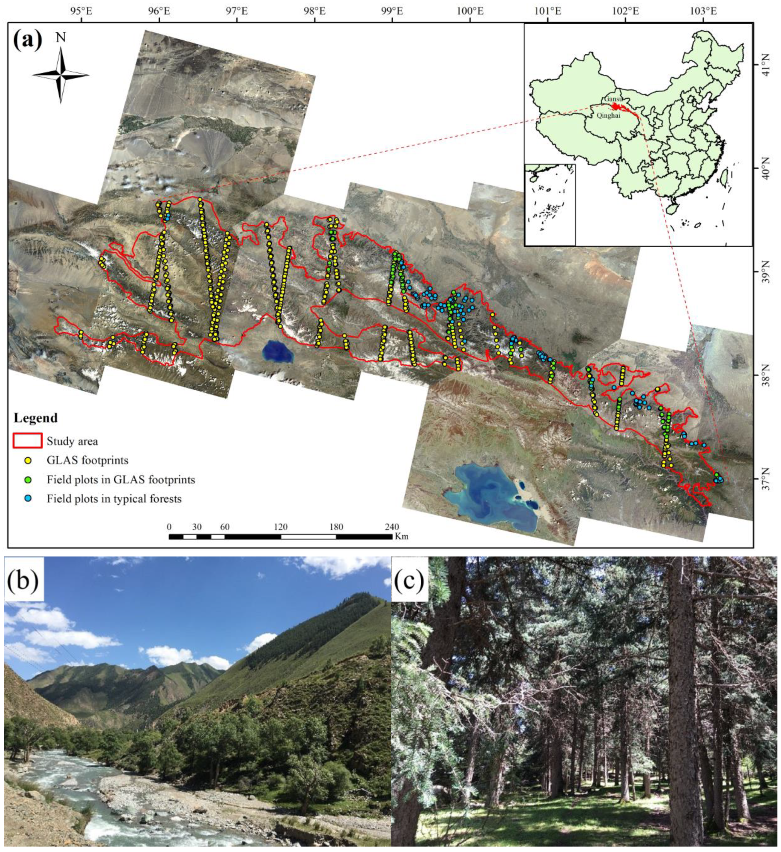
2.1. Study Area
2.2. Field Data
2.3. ICESat/GLAS Data
2.4. Landsat 8 OLI Data
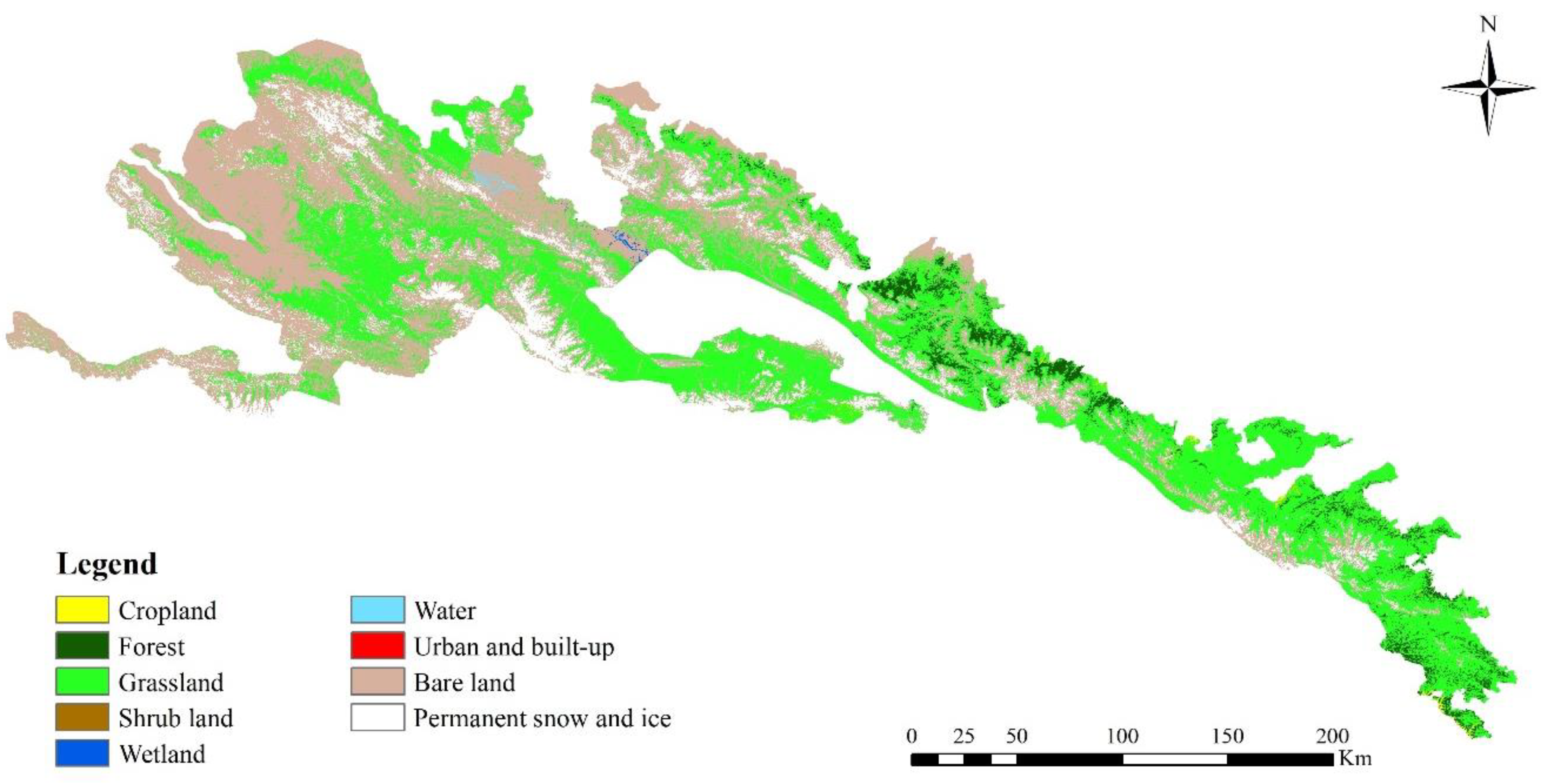
2.5. Land Cover Map
2.6. Environmental Data
3. Methods
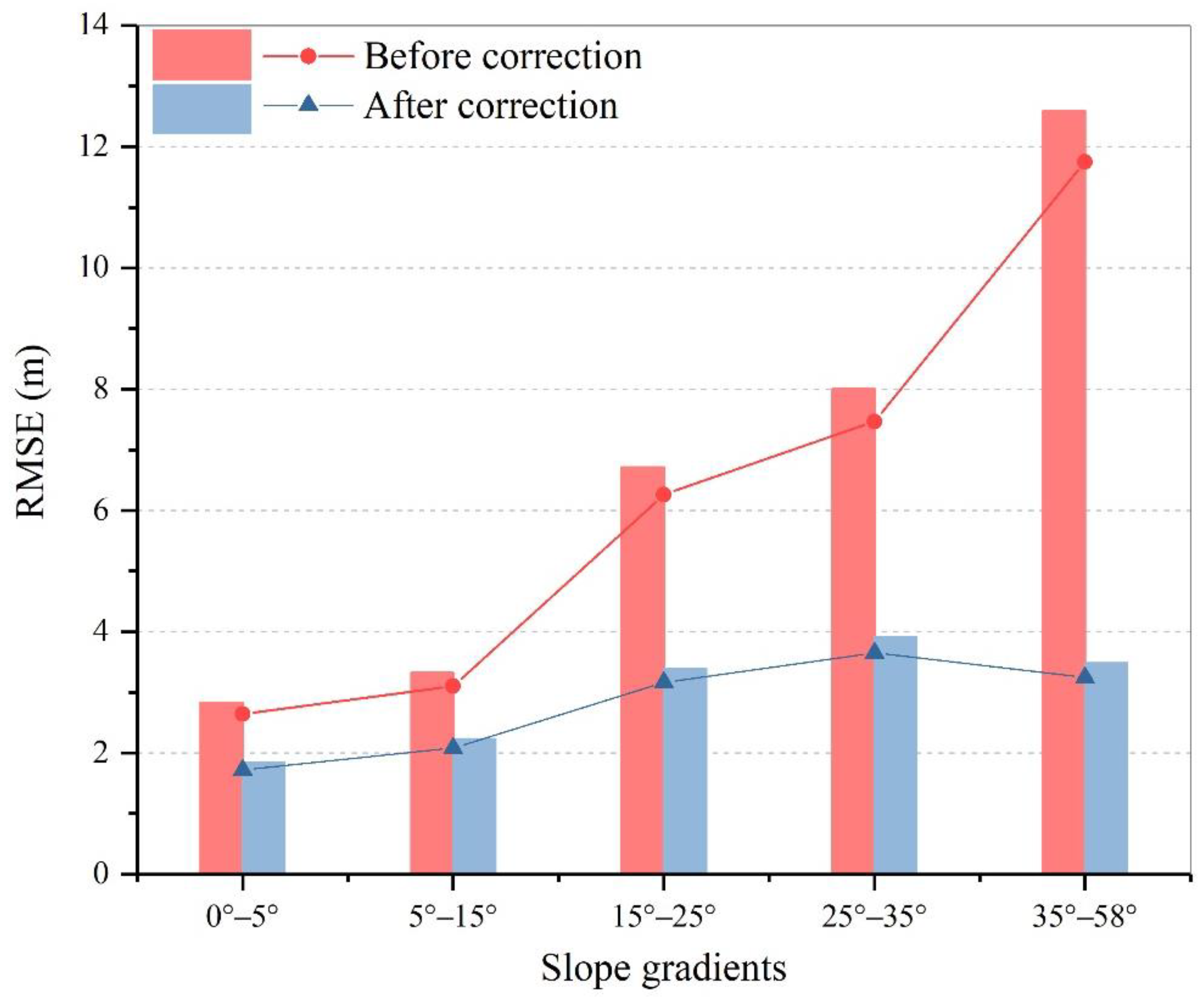
3.1. Deriving Forest Canopy Heights from GLAS Data in Mountainous Areas
3.2. Relating Field-Based AGB to GLAS-Derived Canopy Heights
3.3. Variable Selection for AGB Estimation Modeling
3.4. Algorithms of AGB Estimation Modeling
3.4.1. Extreme Gradient Boosting (XGBoost)
3.4.2. Light Gradient Boosting Machine (LightGBM)
3.4.3. Support Vector Regression (SVR)
3.4.4. Random Forest (RF)
3.5. Accuracy Assessment and Statistical Analysis
4. Results
4.1. GLAS-Derived Canopy Heights Results
4.2. AGB Estimation of GLAS Footprints in Forest Areas
4.3. Variable Selection for AGB Estimation
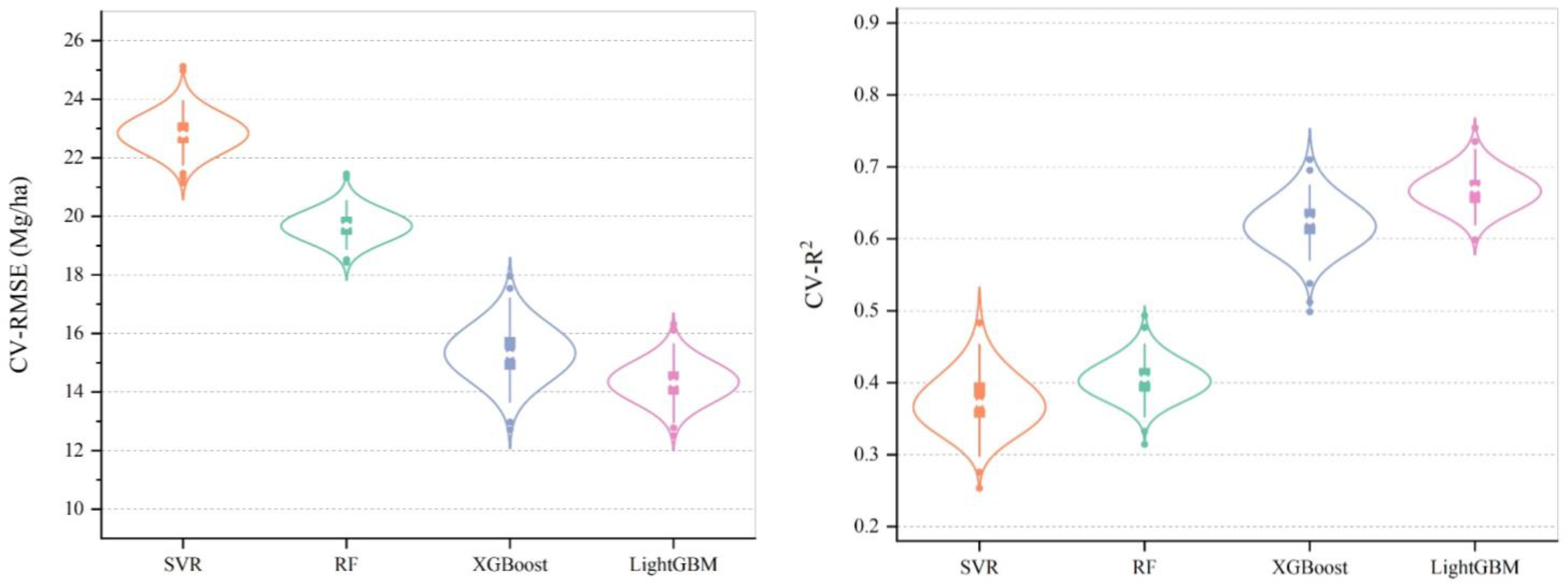
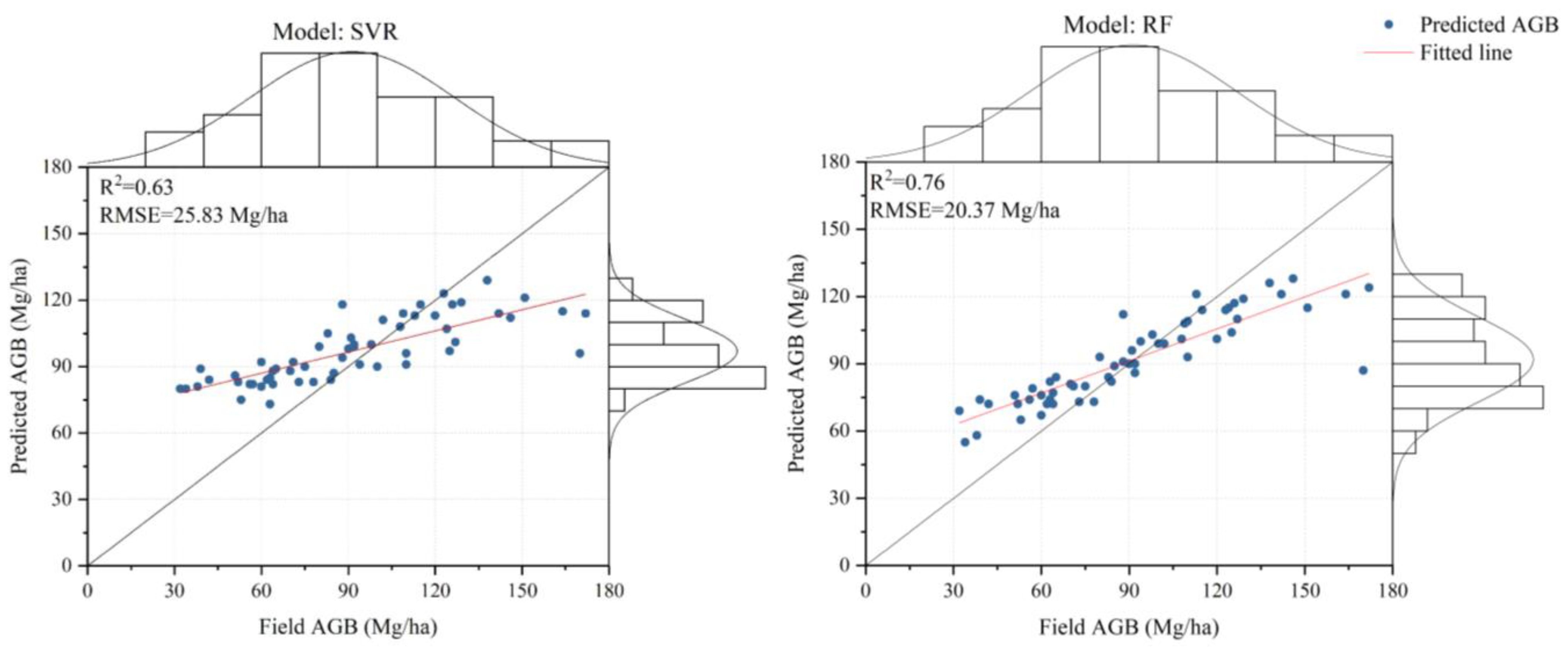
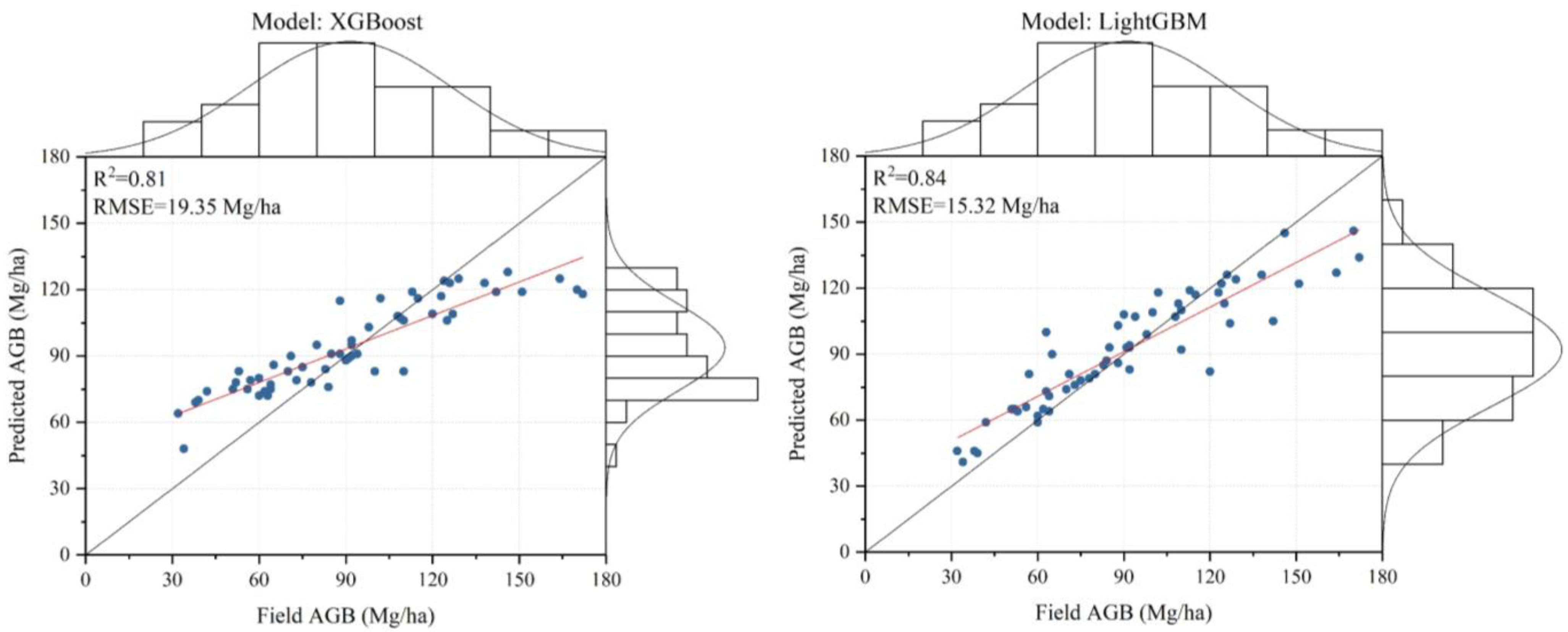
4.4. Comparison of Different AGB Estimation Models
4.5. Forest AGB Mapping
5. Discussion
5.1. Modeling AGB Estimation Using Different Algorithms
5.2. Modeling Variables Selected for AGB Estimation
5.3. Forest Field Survey Data for AGB Estimation
5.4. AGB Estimation in Mountain Forests Using GLAS Data
5.5. Results of Forest AGB Estimation
5.6. Error Analysis
6. Conclusions
Supplementary Materials
Author Contributions
Funding
Institutional Review Board Statement
Informed Consent Statement
Data Availability Statement
Acknowledgments
Conflicts of Interest
References
- Tagesson, T.; Schurgers, G.; Horion, S.; Ciais, P.; Tian, F.; Brandt, M.; Ahlstrom, A.; Wigneron, J.-P.; Ardo, J.; Olin, S.; et al. Recent divergence in the contributions of tropical and boreal forests to the terrestrial carbon sink. Nat. Ecol. Evol. 2020, 4, 202–209. [Google Scholar] [CrossRef]
- Margolis, H.A.; Nelson, R.F.; Montesano, P.M.; Beaudoin, A.; Sun, G.; Andersen, H.-E.; Wulder, M.A. Combining satellite lidar, airborne lidar, and ground plots to estimate the amount and distribution of aboveground biomass in the boreal forest of North America. Can. J. For. Res. 2015, 45, 838–855. [Google Scholar] [CrossRef]
- Zhang, Y.; Liang, S.; Sun, G. Forest Biomass Mapping of Northeastern China Using GLAS and MODIS Data. IEEE J. Sel. Top. Appl. Earth Obs. Remote Sens. 2014, 7, 140–152. [Google Scholar] [CrossRef]
- Lu, D.; Chen, Q.; Wang, G.; Liu, L.; Li, G.; Moran, E. A survey of remote sensing-based aboveground biomass estimation methods in forest ecosystems. Int. J. Digit. Earth 2016, 9, 63–105. [Google Scholar] [CrossRef]
- Zolkos, S.G.; Goetz, S.J.; Dubayah, R. A meta-analysis of terrestrial aboveground biomass estimation using lidar remote sensing. Remote Sens. Environ. 2013, 128, 289–298. [Google Scholar] [CrossRef]
- Sun, X.; Li, G.; Wang, M.; Fan, Z. Analyzing the Uncertainty of Estimating Forest Aboveground Biomass Using Optical Imagery and Spaceborne LiDAR. Remote Sens. 2019, 11, 722. [Google Scholar] [CrossRef]
- Lopez-Serrano, P.M.; Cardenas Dominguez, J.L.; Javier Corral-Rivas, J.; Jimenez, E.; Lopez-Sanchez, C.A.; Jose Vega-Nieva, D. Modeling of Aboveground Biomass with Landsat 8 OLI and Machine Learning in Temperate Forests. Forests 2020, 11, 11. [Google Scholar] [CrossRef]
- de Almeida, C.T.; Galvao, L.S.; de Oliveira Cruz e Aragao, L.E.; Henry Balbaud Ometto, J.P.; Jacon, A.D.; de Souza Pereira, F.R.; Sato, L.Y.; Lopes, A.P.; Lima de Alencastro Graca, P.M.; Silva, C.V.d.J.; et al. Combining LiDAR and hyperspectral data for aboveground biomass modeling in the Brazilian Amazon using different regression algorithms. Remote Sens. Environ. 2019, 232, 111323. [Google Scholar] [CrossRef]
- Fassnacht, F.E.; Hartig, F.; Latifi, H.; Berger, C.; Hernandez, J.; Corvalan, P.; Koch, B. Importance of sample size, data type and prediction method for remote sensing-based estimations of aboveground forest biomass. Remote Sens. Environ. 2014, 154, 102–114. [Google Scholar] [CrossRef]
- Gao, Y.; Lu, D.; Li, G.; Wang, G.; Chen, Q.; Liu, L.; Li, D. Comparative Analysis of Modeling Algorithms for Forest Aboveground Biomass Estimation in a Subtropical Region. Remote Sens. 2018, 10, 627. [Google Scholar] [CrossRef]
- Liu, K.; Wang, J.; Zeng, W.; Song, J. Comparison and Evaluation of Three Methods for Estimating Forest above Ground Biomass Using TM and GLAS Data. Remote Sens. 2017, 9, 341. [Google Scholar] [CrossRef]
- Tien Dat, P.; Yokoya, N.; Xia, J.; Nam Thang, H.; Nga Nhu, L.; Thi Thu Trang, N.; Thi Huong, D.; Thuy Thi Phuong, V.; Tien Duc, P.; Takeuchi, W. Comparison of Machine Learning Methods for Estimating Mangrove Above-Ground Biomass Using Multiple Source Remote Sensing Data in the Red River Delta Biosphere Reserve, Vietnam. Remote Sens. 2020, 12, 1334. [Google Scholar] [CrossRef]
- Bolon-Canedo, V.; Sanchez-Marono, N.; Alonso-Betanzos, A. Feature selection for high-dimensional data. Prog. Artif. Intell. 2016, 5, 65–75. [Google Scholar] [CrossRef]
- Li, Y.; Li, C.; Li, M.; Liu, Z. Influence of Variable Selection and Forest Type on Forest Aboveground Biomass Estimation Using Machine Learning Algorithms. Forests 2019, 10, 1073. [Google Scholar] [CrossRef]
- Fayad, I.; Baghdadi, N.; Guitet, S.; Bailly, J.-S.; Herault, B.; Gond, V.; El Hajj, M.; Dinh Ho Tong, M. Aboveground biomass mapping in French Guiana by combining remote sensing, forest inventories and environmental data. Int. J. Appl. Earth Obs. Geoinf. 2016, 52, 502–514. [Google Scholar] [CrossRef]
- Cao, L.; Pan, J.; Li, R.; Li, J.; Li, Z. Integrating Airborne LiDAR and Optical Data to Estimate Forest Aboveground Biomass in Arid and Semi-Arid Regions of China. Remote Sens. 2018, 10, 532. [Google Scholar] [CrossRef]
- Ke, G.; Meng, Q.; Finley, T.; Wang, T.; Chen, W.; Ma, W.; Ye, Q.; Liu, T.-Y. LightGBM: A Highly Efficient Gradient Boosting Decision Tree. In Proceedings of the 31st Conference on Neural Information Processing Systems, Long Beach, CA, USA, 4–9 December 2017. [Google Scholar]
- Sang, M.; Xiao, H.; Jin, Z.; He, J.; Wang, N.; Wang, W. Improved Mapping of Regional Forest Heights by Combining Denoise and LightGBM Method. Remote Sens. 2023, 15, 5436. [Google Scholar] [CrossRef]
- Hilbert, C.; Schmullius, C. Influence of Surface Topography on ICESat/GLAS Forest Height Estimation and Waveform Shape. Remote Sens. 2012, 4, 2210–2235. [Google Scholar] [CrossRef]
- Wang, J.Y.; Ju, K.J.; Fu, H.E.; Chang, X.X.; He, H.Y. Study on biomass of water conservation forest on North Slope of Qilian Mountains. J. For. Environ. 1998, 18, 319–323. [Google Scholar]
- Abshire, J.B.; Sun, X.L.; Riris, H.; Sirota, J.M.; McGarry, J.F.; Palm, S.; Yi, D.H.; Liiva, P. Geoscience Laser Altimeter System (GLAS) on the ICESat mission: On-orbit measurement performance. Geophys. Res. Lett. 2005, 32, L21S02. [Google Scholar] [CrossRef]
- Park, T.; Kennedy, R.E.; Choi, S.; Wu, J.; Lefsky, M.A.; Bi, J.; Mantooth, J.A.; Myneni, R.B.; Knyazikhin, Y. Application of Physically-Based Slope Correction for Maximum Forest Canopy Height Estimation Using Waveform Lidar across Different Footprint Sizes and Locations: Tests on LVIS and GLAS. Remote Sens. 2014, 6, 6566–6586. [Google Scholar] [CrossRef]
- Chi, H.; Sun, G.; Huang, J.; Guo, Z.; Ni, W.; Fu, A. National Forest Aboveground Biomass Mapping from ICESat/GLAS Data and MODIS Imagery in China. Remote Sens. 2015, 7, 5534–5564. [Google Scholar] [CrossRef]
- Chen, Q. Retrieving vegetation height of forests and woodlands over mountainous areas in the Pacific Coast region using satellite laser altimetry. Remote Sens. Environ. 2010, 114, 1610–1627. [Google Scholar] [CrossRef]
- Garcia, M.; Popescu, S.; Riano, D.; Zhao, K.; Neuenschwander, A.; Agca, M.; Chuvieco, E. Characterization of canopy fuels using ICESat/GLAS data. Remote Sens. Environ. 2012, 123, 81–89. [Google Scholar] [CrossRef]
- Teillet, P.M.; Guindon, B.; Goodenough, D.G. On the slope-aspect correction of multispectral scanner data. Can. J. Remote Sens. 1982, 8, 84–106. [Google Scholar] [CrossRef]
- Turgut, R.; Gunlu, A. Estimating aboveground biomass using Landsat 8 OLI satellite image in pure Crimean pine stands: A case from Turkey. Geocarto Int. 2022, 37, 720–734. [Google Scholar] [CrossRef]
- Rouse, J.W., Jr.; Haas, R.H.; Deering, D.; Schell, J.; Harlan, J.C. Monitoring the Vernal Advancement and Retrogradation (Green Wave Effect) of Natural Vegetation; Final Report; NASA: Goddard Space Flight Centergreenbelt, MI, USA, 1974. [Google Scholar]
- Pearson, R.L.; Miller, L.D. Remote mapping of standing crop biomass for estimation of the productivity of the shortgrass prairie, Pawnee National Grasslands, Colorado. In Proceedings of the Eighth International Symposium on Remote Sensing of Environment, Ann Arbor, MI, USA, 2–6 October 1972. [Google Scholar]
- Srestasathiern, P.; Rakwatin, P. Oil Palm Tree Detection with High Resolution Multi-Spectral Satellite Imagery. Remote Sens. 2014, 6, 9749–9774. [Google Scholar] [CrossRef]
- Huete, A.R. A soil-adjusted vegetation index (SAVI). Remote Sens. Environ. 1988, 25, 295–309. [Google Scholar] [CrossRef]
- Liu, H.Q.; Huete, A. A Feedback Based Modification Of The NDVI To Minimize Canopy Background And Atmospheric Noise. IEEE Trans. Geosci. Remote Sens. 1995, 33, 814. [Google Scholar] [CrossRef]
- Zhong, B.; Yang, A.; Nie, A.; Yao, Y.; Zhang, H.; Wu, S.; Liu, Q. Finer Resolution Land-Cover Mapping Using Multiple Classifiers and Multisource Remotely Sensed Data in the Heihe River Basin. IEEE J. Sel. Top. Appl. Earth Obs. Remote Sens. 2015, 8, 4973–4992. [Google Scholar] [CrossRef]
- Fick, S.E.; Hijmans, R.J. WorldClim 2: New 1-km spatial resolution climate surfaces for global land areas. Int. J. Climatol. 2017, 37, 4302–4315. [Google Scholar] [CrossRef]
- Hayashi, M.; Saigusa, N.; Oguma, H.; Yamagata, Y. Forest canopy height estimation using ICESat/GLAS data and error factor analysis in Hokkaido, Japan. Isprs J. Photogramm. Remote Sens. 2013, 81, 12–18. [Google Scholar] [CrossRef]
- Hu, K.; Liu, Q.; Pang, Y.; Li, M.; Mu, X. Forest canopy height estimation based on ICESat/GLAS data by airborne lidar. Trans. Chin. Soc. Agric. Eng. 2017, 33, 88–95. [Google Scholar]
- Fan, J.Y.; Pan, J.Y. Convergence properties of a self-adaptive Levenberg-Marquardt algorithm under local error bound condition. Comput. Optim. Appl. 2006, 34, 47–62. [Google Scholar] [CrossRef]
- Jiang, F.; Sun, H.; Ma, K.; Fu, L.; Tang, J. Improving aboveground biomass estimation of natural forests on the Tibetan Plateau using spaceborne LiDAR and machine learning algorithms. Ecol. Indic. 2022, 143, 109365. [Google Scholar] [CrossRef]
- Radivojac, P.; Chawla, N.V.; Dunker, A.K.; Obradovic, Z. Classification and knowledge discovery in protein databases. J. Biomed. Inform. 2004, 37, 224–239. [Google Scholar] [CrossRef]
- Sun, H.; Hu, X. Attribute selection for decision tree learning with class constraint. Chemom. Intell. Lab. Syst. 2017, 163, 16–23. [Google Scholar] [CrossRef]
- Chen, C.; Zhang, Q.; Yu, B.; Yu, Z.; Lawrence, P.J.; Ma, Q.; Zhang, Y. Improving protein-protein interactions prediction accuracy using XGBoost feature selection and stacked ensemble classifier. Comput. Biol. Med. 2020, 123, 103899. [Google Scholar] [CrossRef]
- Friedman, J.H. Greedy function approximation: A gradient boosting machine. Ann. Stat. 2001, 29, 1189–1232. [Google Scholar] [CrossRef]
- Sheridan, R.P.; Wang, W.M.; Liaw, A.; Ma, J.; Gifford, E.M. Extreme Gradient Boosting as a Method for Quantitative Structure-Activity Relationships. J. Chem. Inf. Model. 2016, 56, 2353–2360. [Google Scholar] [CrossRef]
- Machado, M.R.; Karray, S.; de Sousa, I.T. LightGBM: An Effective Decision Tree Gradient Boosting Method to Predict Customer Loyalty in the Finance Industry. In Proceedings of the 14th International Conference on Computer Science and Education (ICCSE 2019), Toronto, ON, Canada, 19–21 August 2019; pp. 1111–1116. [Google Scholar]
- Chen, P.H.; Lin, C.J.; Schölkopf, B. A tutorial on support vector machines. Appl. Stoch. Models Bus. Ind. 2005, 21, 111–136. [Google Scholar] [CrossRef]
- Zhao, K.; Popescu, S.; Meng, X.; Pang, Y.; Agca, M. Characterizing forest canopy structure with lidar composite metrics and machine learning. Remote Sens. Environ. 2011, 115, 1978–1996. [Google Scholar] [CrossRef]
- Breiman, L. Bagging predictors. Mach. Learn. 1996, 24, 123–140. [Google Scholar] [CrossRef]
- Breiman, L. Random forests. Mach. Learn. 2001, 45, 5–32. [Google Scholar] [CrossRef]
- Zhang, J.; Huang, S.; Hogg, E.H.; Lieffers, V.; Qin, Y.; He, F. Estimating spatial variation in Alberta forest biomass from a combination of forest inventory and remote sensing data. Biogeosciences 2014, 11, 2793–2808. [Google Scholar] [CrossRef]
- Wu, C.; Shen, H.; Shen, A.; Deng, J.; Gan, M.; Zhu, J.; Xu, H.; Wang, K. Comparison of machine-learning methods for above-ground biomass estimation based on Landsat imagery. J. Appl. Remote Sens. 2016, 10, 035010. [Google Scholar] [CrossRef]
- Tien Dat, P.; Nga Nhu, L.; Nam Thang, H.; Luong Viet, N.; Xia, J.; Yokoya, N.; Tu Trong, T.; Hong Xuan, T.; Lap Quoc, K.; Takeuchi, W. Estimating Mangrove Above-Ground Biomass Using Extreme Gradient Boosting Decision Trees Algorithm with Fused Sentinel-2 and ALOS-2 PALSAR-2 Data in Can Gio Biosphere Reserve, Vietnam. Remote Sens. 2020, 12, 777. [Google Scholar] [CrossRef]
- Luo, M.; Wang, Y.; Xie, Y.; Zhou, L.; Qiao, J.; Qiu, S.; Sun, Y. Combination of Feature Selection and CatBoost for Prediction: The First Application to the Estimation of Aboveground Biomass. Forests 2021, 12, 216. [Google Scholar] [CrossRef]
- Ye, Q.; Yu, S.; Liu, J.; Zhao, Q.; Zhao, Z. Aboveground biomass estimation of black locust planted forests with aspect variable using machine learning regression algorithms. Ecol. Indic. 2021, 129, 107948. [Google Scholar] [CrossRef]
- Wai, P.; Su, H.; Li, M. Estimating Aboveground Biomass of Two Different Forest Types in Myanmar from Sentinel-2 Data with Machine Learning and Geostatistical Algorithms. Remote Sens. 2022, 14, 2146. [Google Scholar] [CrossRef]
- Uniyal, S.; Purohit, S.; Chaurasia, K.; Amminedu, E.; Rao, S.S. Quantification of carbon sequestration by urban forest using Landsat 8 OLI and machine learning algorithms in Jodhpur, India. Urban For. Urban Green. 2022, 67, 127445. [Google Scholar] [CrossRef]
- Rana, P.; Popescu, S.; Tolvanen, A.; Gautam, B.; Srinivasan, S.; Tokola, T. Estimation of tropical forest aboveground biomass in Nepal using multiple remotely sensed data and deep learning. Int. J. Remote Sens. 2023, 44, 5147–5171. [Google Scholar] [CrossRef]
- Wang, Z.; Yi, L.; Xu, W.; Zheng, X.; Xiong, S.; Bao, A. Integration of UAV and GF-2 Optical Data for Estimating Aboveground Biomass in Spruce Plantations in Qinghai, China. Sustainability 2023, 15, 9700. [Google Scholar] [CrossRef]
- Zhang, Y.; Ma, J.; Liang, S.; Li, X.; Li, M. An Evaluation of Eight Machine Learning Regression Algorithms for Forest Aboveground Biomass Estimation from Multiple Satellite Data Products. Remote Sens. 2020, 12, 4015. [Google Scholar] [CrossRef]
- LeCun, Y.; Bengio, Y.; Hinton, G. Deep learning. Nature 2015, 521, 436–444. [Google Scholar] [CrossRef] [PubMed]
- Bengio, Y.; Delalleau, O. On the Expressive Power of Deep Architectures. In Proceedings of the 22nd International Conference on Algorithmic Learning Theory (ALT 2011), Espoo, Finland, 5–7 October 2011; pp. 18–36. [Google Scholar]
- Ghosh, S.M.; Behera, M.D. Aboveground biomass estimates of tropical mangrove forest using Sentinel-1 SAR coherence data-The superiority of deep learning over a semi-empirical model. Comput. Geosci. 2021, 150, 104737. [Google Scholar] [CrossRef]
- Narine, L.L.; Popescu, S.C.; Malambo, L. Synergy of ICESat-2 and Landsat for Mapping Forest Aboveground Biomass with Deep Learning. Remote Sens. 2019, 11, 1503. [Google Scholar] [CrossRef]
- Yu, X.; Ge, H.; Lu, D.; Zhang, M.; Lai, Z.; Yao, R. Comparative Study on Variable Selection Approaches in Establishment of Remote Sensing Model for Forest Biomass Estimation. Remote Sens. 2019, 11, 1437. [Google Scholar] [CrossRef]
- Roy, D.P.; Wulder, M.A.; Loveland, T.R.; Woodcock, C.E.; Allen, R.G.; Anderson, M.C.; Helder, D.; Irons, J.R.; Johnson, D.M.; Kennedy, R.; et al. Landsat-8: Science and product vision for terrestrial global change research. Remote Sens. Environ. 2014, 145, 154–172. [Google Scholar] [CrossRef]
- Chrysafis, I.; Mallinis, G.; Gitas, I.; Tsakiri-Strati, M. Estimating Mediterranean forest parameters using multi seasonal Landsat 8 OLI imagery and an ensemble learning method. Remote Sens. Environ. 2017, 199, 154–166. [Google Scholar] [CrossRef]
- Han, H.; Wan, R.; Li, B. Estimating Forest Aboveground Biomass Using Gaofen-1 Images, Sentinel-1 Images, and Machine Learning Algorithms: A Case Study of the Dabie Mountain Region, China. Remote Sens. 2022, 14, 176. [Google Scholar] [CrossRef]
- Strunk, J.; Temesgen, H.; Andersen, H.-E.; Flewelling, J.P.; Madsen, L. Effects of lidar pulse density and sample size on a model-assisted approach to estimate forest inventory variables. Can. J. Remote Sens. 2012, 38, 644–654. [Google Scholar] [CrossRef]
- Paine, C.E.T.; Baraloto, C.; Diaz, S. Optimal strategies for sampling functional traits in species-rich forests. Funct. Ecol. 2015, 29, 1325–1331. [Google Scholar] [CrossRef]
- Milenkovic, M.; Schnell, S.; Holmgren, J.; Ressl, C.; Lindberg, E.; Hollaus, M.; Pfeifer, N.; Olsson, H. Influence of footprint size and geolocation error on the precision of forest biomass estimates from space-borne waveform LiDAR. Remote Sens. Environ. 2017, 200, 74–88. [Google Scholar] [CrossRef]
- Tian, X.; Yan, M.; van der Tol, C.; Li, Z.; Su, Z.; Chen, E.; Li, X.; Li, L.; Wang, X.; Pan, X.; et al. Modeling forest above-ground biomass dynamics using multi-source data and incorporated models: A case study over the qilian mountains. Agric. For. Meteorol. 2017, 246, 1–14. [Google Scholar] [CrossRef]
- Xu, N.; Ma, X.; Ma, Y.; Zhao, P.; Yang, J.; Wang, X.H. Deriving Highly Accurate Shallow Water Bathymetry From Sentinel-2 and ICESat-2 Datasets by a Multitemporal Stacking Method. IEEE J. Sel. Top. Appl. Earth Obs. Remote Sens. 2021, 14, 6677–6685. [Google Scholar] [CrossRef]


| Source | Label | Description |
|---|---|---|
| Original Band | Band 2 | Blue (B) |
| Band 3 | Green (G) | |
| Band 4 | Red (R) | |
| Band 5 | Near Infrared (NIR) | |
| Band 6 | Shortwave Infrared (SWIR1) | |
| Band 7 | Shortwave Infrared (SWIR2) | |
| Vegetation Indices (VIs) | NDVI [28] | |
| SR [29] | ||
| TVI [30] | ||
| SAVI [31] | , L = 0.5 | |
| EVI [32] |
| Land-Use Type | Ground Truth (%) | Producer Accuracy (%) | |||||
|---|---|---|---|---|---|---|---|
| Cropland | Forest | Grassland | Water | Bare Land | |||
| Land cover map (%) | Cropland | 21.24 | 0.00 | 2.26 | 0.26 | 0.00 | 21.24 |
| Forest | 3.15 | 95.34 | 36.28 | 0.00 | 0.67 | 95.34 | |
| Grassland | 75.61 | 3.76 | 61.46 | 6.15 | 1.72 | 61.46 | |
| Water | 0.00 | 0.06 | 0.00 | 69.31 | 0.00 | 69.31 | |
| Bare land | 0.00 | 0.84 | 0.00 | 24.28 | 97.61 | 97.61 | |
| User accuracy (%) | 61.59 | 93.53 | 58.39 | 98.69 | 95.99 | —— | |
| Algorithm | Learning Rate | Min_Samples_Leaf Min_Child_Weight | Gamma | Max_Depth/Max Feature | n_Estimators/n_Iteration/or C Value |
|---|---|---|---|---|---|
| XGBoost | 1 | 1 | 0 | 6 | 100 |
| LightGBM | 2 | 20 | NA | 6 | 200 |
| SVR | 0.1 | NA | 1000 | NA | 1 |
| RF | NA | 1 | NA | 15 | 50 |
| Elevation Gradient | Model | p Value | R2 | Adjusted R2 | Displayed Formula |
| 1770–2770 m | Quadratic | 0.004 | 0.67 | 0.60 | *Y = −204.42 + 59.52X − 2.62X2 |
| 2770–3770 m | Cubic | 0.00004 | 0.69 | 0.66 | Y = 6.97X + 0.46X2−0.02X3 + 6.48 |
| 3770–4770 m | Cubic | 0.00001 | 0.78 | 0.73 | Y = 23.79X − 3.28X2 + 0.19X3 − 11.22 |
| Elevation Gradient | Number | Minimum | Maximum | Median | Mean | Standard Deviation |
|---|---|---|---|---|---|---|
| 1770–2770 m | 12 | 64.28 | 176.14 | 78.57 | 91.67 | 38.04 |
| 2770–3770 m | 90 | 18.15 | 184.09 | 76.54 | 81.46 | 34.25 |
| 3770–4770 m | 4 | 11.09 | 64.78 | 48.72 | 43.11 | 19.91 |
| Dataset | Variable | Dataset | Variable |
|---|---|---|---|
| Original Band | Band4 | WorldClim | Bio11 |
| Band5 | Bio12 | ||
| Band6 | Bio13 | ||
| Band7 | Bio15 | ||
| WorldClim | Bio1 | Bio16 | |
| Bio2 | Bio17 | ||
| Bio3 | VIs | EVI | |
| Bio4 | DEM | Elevation | |
| Bio5 | Slope | ||
| Bio6 | Aspect | ||
| Bio7 | Soil | Soil Texture |
| No. | Modeling Approach | Data Sources | Forest Type | The Optimal Model and Its Performance | Year | Reference | ||
|---|---|---|---|---|---|---|---|---|
| Optimal Model | R2 | RMSE (Mg/ha) | ||||||
| 1 | Non-spatial and spatial regression models Spatial interpolation Random Forest (RF) | Forest inventory data ICESat/GLAS Climatic variables Elevation | Boreal forests | RF | 0.62 | 47.03 | 2014 | [49] |
| 2 | Support Vector Regression (SVR) k-Nearest Neighbor (kNN) Stepwise Linear Regression (SLR) Random Forest (RF) Stochastic Gradient Boosting (SGB) | Field survey data Landsat 5 TM | Subtropical forests | RF | 0.63 | 26.44 | 2016 | [50] |
| 3 | Random Forest (RF) Support Vector Regression (SVR) | Forest inventory data Landsat 8 OLI Climatic variables Topographic variables | Temperate forests | SVR | 0.8 | 8.20 | 2020 | [7] |
| 4 | Extreme Gradient Boosting (XGBoost) Support Vector Regression (SVR) Gradient Boosting Regression (GBR) Random Forest (RF) Gaussian Process Regression (GPR) | Field survey data Sentinel-2 MSI ALOS-2 PALSAR-2 | Mangrove | XGBR | 0.805 | 28.13 | 2020 | [51] |
| 5 | Random Forest Regression (RFR) Extreme Gradient Boosting (XGBoost) Categorical Boosting (CatBoost) | National Forest Continuous Inventory (NFCI) data Landsat 8 OLI Topographic variables Canopy density | Temperate forests | CatBoost | 0.73 | 25.77 | 2021 | [52] |
| 6 | Random Forest (RF) Support Vector Regression (SVR) Artificial Neural Network (ANN) | Field survey data Landsat 8 OLI Aspect | Planted forests | RF | 0.8519 | 12.552 | 2021 | [53] |
| 7 | Kriging algorithms Stochastic Gradient Boosting (SGB) Random Forest (RF) | Field survey data Sentinel-2 image Terrain factors (elevation, slope, aspect) | Tropical forests | RF-based ordinary Kriging | 0.47 | 24.91 | 2022 | [54] |
| 8 | Random Forest (RF) Support Vector Regression (SVR) Extreme Gradient Boosting (XGBoost) k-Nearest Neighbor (kNN) | Field survey data Landsat 8 OLI | Urban forests | XGBoost | 0.89 | 14.08 | 2022 | [55] |
| 9 | Random Forest (RF) Stacked Autoencoder (SAE) network Extremely Randomized Trees (ERT) Weighted Least Squares (WLS) | Field survey data Airborne Laser Scanning (ALS) RapidEye satellite image Landsat 5 TM | Tropical forests | SAE | 0.8 | 54.01 | 2023 | [56] |
| 10 | Random Forest (RF) Support Vector Regression (SVR) Ordinary Least-Squares (OLS) Artificial Neural Network(ANN) | Unmanned Aerial Vehicle (UAV) GF-2 image | Planted forests | RF | 0.86 | 1.75 | 2023 | [57] |
Disclaimer/Publisher’s Note: The statements, opinions and data contained in all publications are solely those of the individual author(s) and contributor(s) and not of MDPI and/or the editor(s). MDPI and/or the editor(s) disclaim responsibility for any injury to people or property resulting from any ideas, methods, instructions or products referred to in the content. |
© 2024 by the authors. Licensee MDPI, Basel, Switzerland. This article is an open access article distributed under the terms and conditions of the Creative Commons Attribution (CC BY) license (https://creativecommons.org/licenses/by/4.0/).
Share and Cite
Song, J.; Liu, X.; Adingo, S.; Guo, Y.; Li, Q. A Comparative Analysis of Remote Sensing Estimation of Aboveground Biomass in Boreal Forests Using Machine Learning Modeling and Environmental Data. Sustainability 2024, 16, 7232. https://doi.org/10.3390/su16167232
Song J, Liu X, Adingo S, Guo Y, Li Q. A Comparative Analysis of Remote Sensing Estimation of Aboveground Biomass in Boreal Forests Using Machine Learning Modeling and Environmental Data. Sustainability. 2024; 16(16):7232. https://doi.org/10.3390/su16167232
Chicago/Turabian StyleSong, Jie, Xuelu Liu, Samuel Adingo, Yanlong Guo, and Quanxi Li. 2024. "A Comparative Analysis of Remote Sensing Estimation of Aboveground Biomass in Boreal Forests Using Machine Learning Modeling and Environmental Data" Sustainability 16, no. 16: 7232. https://doi.org/10.3390/su16167232
APA StyleSong, J., Liu, X., Adingo, S., Guo, Y., & Li, Q. (2024). A Comparative Analysis of Remote Sensing Estimation of Aboveground Biomass in Boreal Forests Using Machine Learning Modeling and Environmental Data. Sustainability, 16(16), 7232. https://doi.org/10.3390/su16167232