Evaluating the Performance of Protective Barriers against Debris Flows Using Coupled Eulerian Lagrangian and Finite Element Analyses

Abstract

Protective structures are critical in mitigating the dangers posed by debris flows. However, evaluating their performance remains a challenge, especially considering boulder transport in complex 3D terrains. This study introduces a comprehensive methodology to appraise the effectiveness of protective structures under the impact of debris flows for real-world conditions along the Hobart Rivulet in Tasmania, Australia. The validation of the Coupled Eulerian-Lagrangian (CEL) model against experimental data demonstrates its high accuracy in predicting flow dynamics and impact forces, whereby flow velocities are estimated for subsequent Finite Element (FE) analyses. By simulating boulder-barrier interactions, weak points in I-beam post barriers are identified, with a broad investigation of the effects on the barrier performance under various conditions. The establishment of a 3D CEL model to assess the interactions between debris flow, boulders, and I-beam post barriers in a complex rivulet terrain is of particular significance. Through CEL and FE analyses, various aspects of debris flow-structure interactions are presented, including structural failure, impact force, and boulder velocity. The findings provide insights into the suitability of various numerical methods to assess the performance of protective measures in real-world scenarios.

1. Introduction

Debris flows present considerable threats to communities and the environment, particularly when transporting media such as boulders and wood [1,2]. Mitigating debris flow risks typically involves constructing protective structures tailored to address specific challenges posed by these natural hazards. Various protective measures are employed to mitigate debris flow risks depending on the local setting and the purpose of the countermeasures [3,4,5,6]. Traditional measures include retaining walls and open rigid barriers, while more advanced solutions involve flexible netting systems. Rigid barriers, such as concrete or steel barriers, are designed to intercept and contain falling debris, thereby reducing downstream damage, proving particularly effective in mountainous areas. I-beam barriers are favoured for their adaptability and cost-effectiveness and are widely implemented in the city of Hobart, Tasmania. The effectiveness of such structures depends on their capacity to withstand impact forces, kinetic energy, and the dynamic forces exerted by debris flows and transported materials. Assessing the performance of these structures is crucial for optimising their design and the effectiveness of mitigation measures.

Numerical methods present a robust and efficient tool for exploring the characteristics of flow impact, finding extensive applications in predicting and dissecting debris flow dynamics [7,8,9,10,11]. Various investigations focus on specific fluid mechanics properties of debris flow within intricate three-dimensional terrains through the application of these methodologies to real-world scenarios [12,13,14,15]. For instance, Zhang et al. [9] introduced a three-dimensional CFD code based on the Finite Difference Method (FDM) to simulate debris flow runout in Xiaojia Gully in China, providing an approach for risk management and engineering designs. Yu et al. [16] developed a three-dimensional Finite Volume Method (FVM) scheme using Navier–Stokes equations and the Bingham–Papanastasiou rheology model to predict mud flow from dam failures and applied to scenarios including the 2019 Feijão tailing dam failure in Brazil, demonstrating its utility for disaster early warning and emergency response. Guo et al. [13] modelled the dynamic processes of the 2013 Wulipo landslides-induced debris flow using the Discrete Element Method (DEM), highlighting the significance of considering topographic and entrainment effects for simulating real-world applications. Zhou et al. [17] conducted a back-analysis of an earthquake-induced debris flow event in Donghekou, China, using a coupled model based on the FDM and DEM, attributing slope failure to elevation-induced amplification, with a relatively low initial velocity triggering the sliding mass movement.

Several studies have used Finite Elements (FE) and Computational Fluid Dynamics (CFD) to analyse how protective structures respond to varying loads, aiding in the development of more effective protective measures [18,19,20,21,22]. Similarly, debris flow–structure interactions are key to assessing the potential impacts based on real events. Chen et al. [23] studied runout characteristics and debris flow-check dam interactions using a combined approach of the Finite Element Method (FEM) and the Smoothed Particle Hydrodynamics (SPH) method based on the 3D topography of the 1985 Stava debris flow. Kefayati et al. [24] investigated a real debris dam failure case in Anhui, China, employing the Lattice Boltzmann method (LBM) combined with FDM. A few studies have incorporated numerical models considering the transportation dynamics of rock-dominant materials [25,26,27]. Current studies have focused on performance assessments for protective barriers against debris flow impacts [22,28,29,30]. Sun et al. [30] investigated the impact of different baffle positions on debris flow protection by using a three-dimensional DEM model, finding that baffles in the transit area are more effective, with the optimal arrangement determined through orthogonal design analysis. Kokuryo et al. [29] introduced a safety assessment method for steel open dams using the energy constant law, ensuring that the ultimate strength exceeds the required strength against large-scale debris flow loads. As one of the powerful numerical modelling approaches, some studies presented the capability of the Coupled Eulerian Lagrangian (CEL) method in dealing with complex debris flow and structural interactions [11,21,27,31]. However, there is still a lack of research using the CEL modelling approach to evaluate the performance of protective structures designed to mitigate debris flow risks by analysing the impact characteristics of boulders transported by debris flow in complex 3D terrains.

Tasmania, Australia, with its diverse geological and topographical features, is particularly prone to various natural hazards, including debris flow, necessitating comprehensive research to investigate its impacts [32]. Historical events, such as the 2018 Kunanyi debris flows, have caused significant environmental damage and disruptions to transportation networks, highlighting the vulnerability of local communities and the critical importance of effective mitigation strategies [32,33,34]. To address this gap in evaluating the barrier performance in real-world scenarios, this study presents a procedural assessment for protective structures, with a specific focus on the application of modelling flow–boulder–barrier interactions within the CEL modelling framework. The proposed CEL model builds on previous research that considered boulder transport on the complex terrain of an Australian rivulet [27], with attention given to an existing protective I-beam post barrier constructed along one of the primary watercourses in the city. Validation is provided through the simulation of large-scale debris flow experiments. Debris flow dynamics are investigated by estimating flow velocities at different locations along the flow path of the study area. A series of analyses were undertaken to model boulder–barrier interactions (FE models) under various conditions, identifying the weak point of the selected I-beam barrier and investigating factors that impacted the structural performance. By conducting benchmark simulations of debris flow–boulder–barrier interactions (CEL models), the performance of I-beam barriers was evaluated, providing an increased understanding of employing numerical approaches in enhancing structural resilience and optimising barrier design against debris flow impacts.

2. Methodology

2.1. Coupled Eulerian–Lagrangian Method (CEL)

The Coupled Eulerian–Lagrangian (CEL) method is a widely used computational approach in fluid dynamics for simulating fluid–structure interactions. This technique effectively combines Eulerian and Lagrangian reference frames for complex scenarios involving large deformations, which is particularly valuable in geoscience and geotechnical applications [31,35,36,37]. Previous studies have extensively evaluated the CEL method, identifying its strengths, limitations, and efficacy in simulating fluid–solid interactions for debris flow risk mitigation [11,21,27].

In CEL, the behaviour of volumetric elements over time is described using two distinct approaches: Lagrangian and Eulerian descriptions. Generally, the Eulerian approach is utilised to mesh elements undergoing large deformations, while the Lagrangian approach is employed for solid body objects (either rigid or deformable). During the Eulerian step, the movement of material through the mesh is monitored using an Eulerian Volume Fraction (EVF), which indicates the proportion of material within each element. In the Lagrangian step, the deformed mesh is mapped back to the original fixed mesh, with the EVF of each element determined based on the volume of material transported between adjacent elements. The interaction between Eulerian and Lagrangian materials is enforced through a penalty contact method, allowing Lagrangian elements to move through the Eulerian domain until encountering an Eulerian element with a non-zero EVF. This contact algorithm accommodates slight penetration of Eulerian material into Lagrangian elements and automatically tracks the interface during simulations [15,19]. For a detailed algorithm of this technique, refer to the papers published by the authors [11,27]. Additional exploration of the principles and governing equations of this method provides further insight into its applicability in fluid flow scenarios [31,38].

2.2. Rheological Model of Debris Flow

Debris flow materials often exhibit complex behaviours such as elastoplasticity or viscoplasticity, which can be modelled using various rheological approaches like the Bingham model [39,40], the Herschel–Bulkley model [41,42], and the Voellmy–Salm model [43,44]. Numerous studies have explored the intricate behaviours of debris flows, analysing their solid-like and fluid-like phases to better understand their dynamic characteristics across different flow conditions [45,46]. This study simulates interactions among debris flow, boulders, and barriers by explicitly combining large solid object debris transported by debris flow fluids rather than being absorbed within the debris flow fluid rheology, as is the case with small-scale media. To capture the fluid-like nature of debris flows, the Bingham or Herschel-Bulkley models are commonly employed to simulate debris flows as non-Newtonian fluids. In this study, the Bingham model is adopted due to its proven efficacy in simulating debris flow–barrier interactions [11,47], and its successful application in back-analyses of regional debris flow events [48,49]. In ABAQUS, the Bingham model can be reformulated into the Herschel-Bulkley model with an equivalent fluid viscosity. Such a model is characterised by a linear relationship between the shear stress and shear strain rate, where shear stress increases proportionally with the shear strain rate after surpassing a critical yield stress. The yield stress is the threshold stress required to initiate continuous flow, marking the point at which debris begins to move [27,50,51].

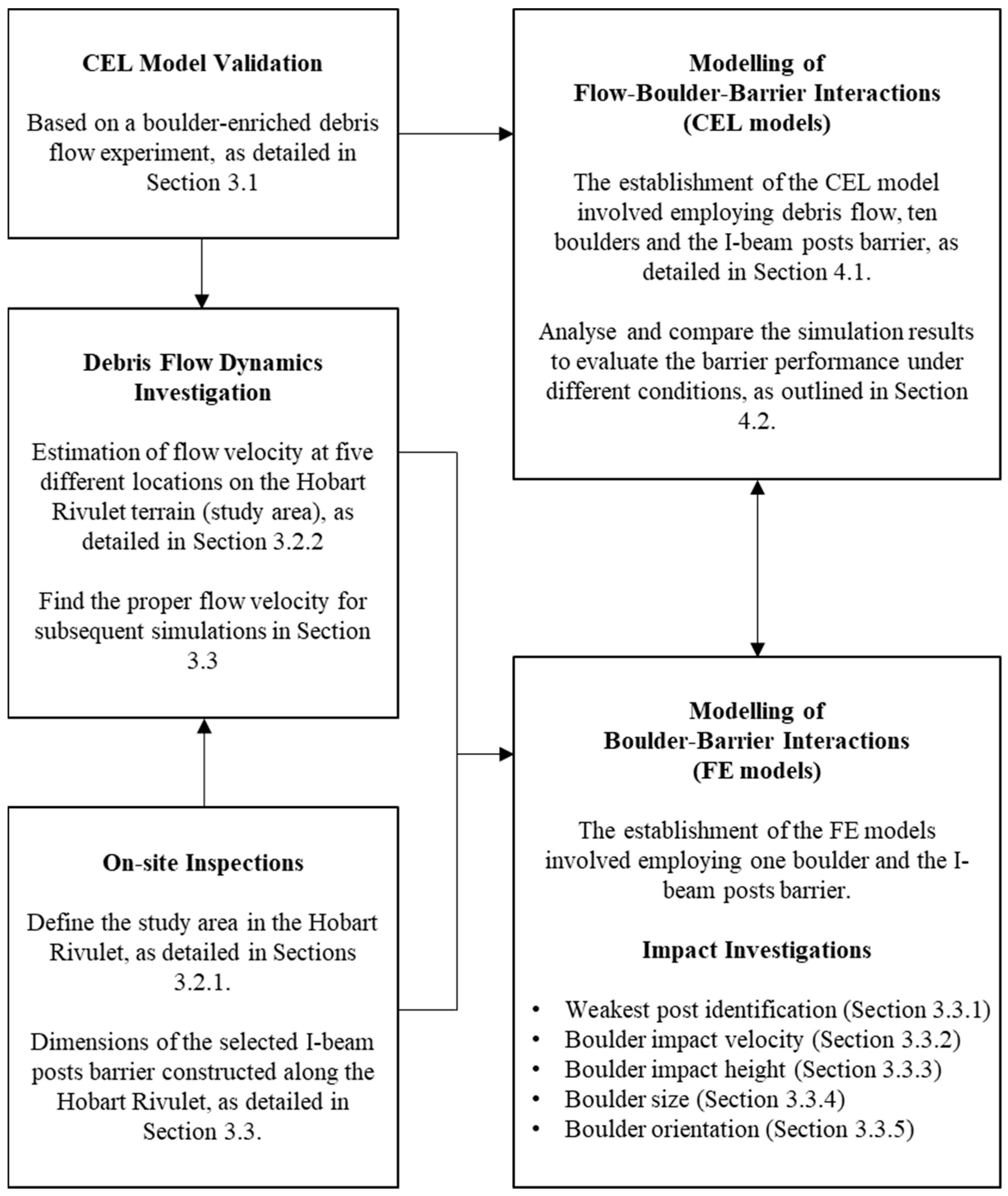
3. Validation and Investigation

This section presents the validation of the proposed CEL method by replicating debris flow experimental results [52]. Subsequently, the CEL model is tailored to the specific area of Hobart Rivulet and designed to simulate debris flow dynamics, thereby enabling the estimation of flow velocities at different locations along the rivulet. Focusing on a specific case of an I-beam post barrier based on on-site inspections, a series of simulations are undertaken to model the I-beam post barrier subjected to boulder impact, with the performance of the barrier evaluated under various conditions. Figure 1 illustrates an overview of the proposed procedure for the performance assessment in this study. Subsequent sections provide detailed explanations along with the presentation and discussion of the simulation results.

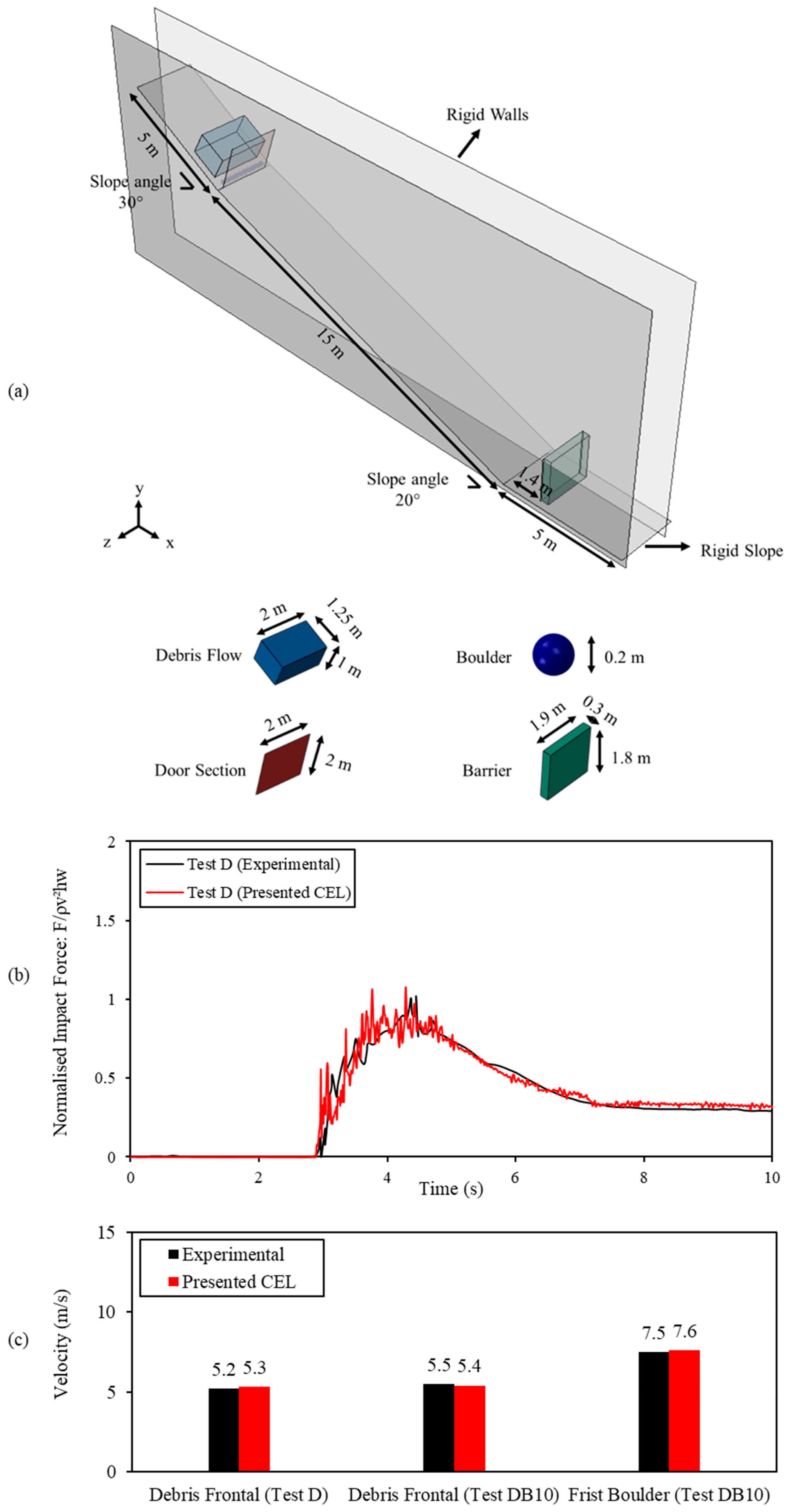
3.1. Model Validation

To evaluate the effectiveness of incorporating boulders into the CEL model for simulating debris flow and barrier interactions, a comparative analysis was performed with reference to a well-known large-scale experiment combining debris flows and transported media conducted by Ng et al. [52]. The CEL model features a 25 m rigid slope with two channel walls, a door section, a debris flow segment, ten boulders, and a barrier to measure impact force, as depicted in Figure 2a. The slope is divided into sections of 5 m, 15 m, and 5 m, with slope angles of 30°, 20°, and 0°, respectively. The channel is 2 m wide, and the barrier dimensions are 1.8 m in height, 1.9 m in width, and 0.3 m in thickness. The debris flow is characterised by dimensions of 2 m × 1.25 m × 1 m, totalling 2.5 m³ in volume, and each boulder has a diameter of 0.2 m. In Test DB10, ten boulders are placed 16.4 m behind the door section on the upper slope. A total simulation time of 15 s is required, with the door removed at 5 s to release the debris flow and boulders. Test D is conducted in the absence of boulders. Figure 2b compares the temporal evolution of impact forces from Test D with the experimental results from Ng et al. [52]. Similarly, Figure 2c shows the comparisons of debris frontal and first arrival boulder velocities between the CEL simulations and physical experiments. The CEL simulation results demonstrate a robust alignment with experimental results in capturing the effects of debris flow and boulders. A comprehensive validation analysis is detailed in Sha et al. [27].

3.2. Estimating Flow Velocities at Different Locations on Hobart Rivulet Terrain

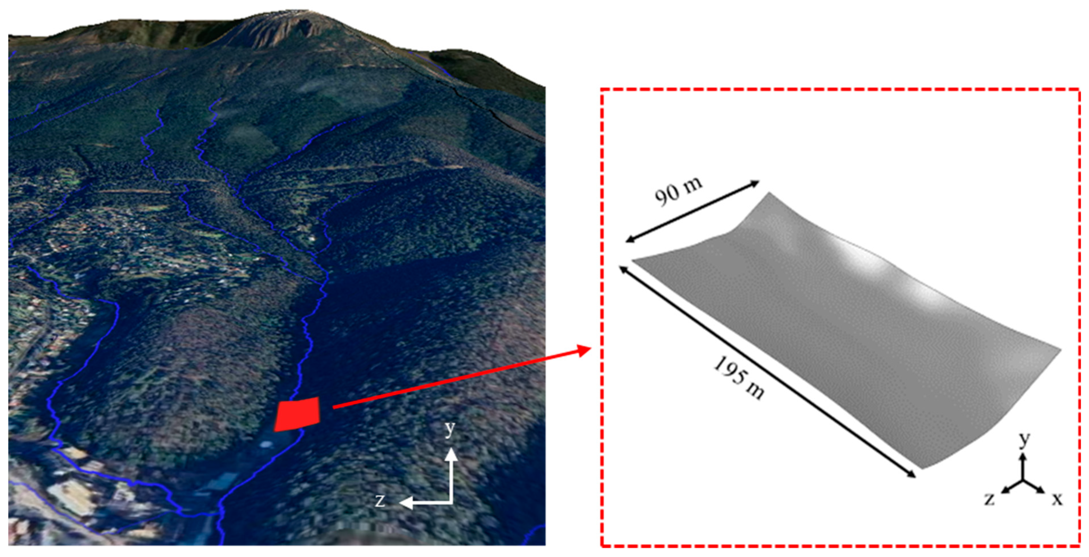
3.2.1. Study Area

The Hobart Rivulet in Tasmania, Australia, is crucial for controlling stormwater and floodwaters for the city of Hobart [32]. Originating at an elevation of 700 m within Kunanyi (Mount Wellington) Park, it flows from Strickland Falls through South Hobart, the city centre, and ultimately into the River Derwent. A key segment of the rivulet, marked in red in Figure 3, measures 195 m in length and 90 m in width, serving as a point of construction. This area is particularly important within the debris flow protection system, which has barriers currently in place to mitigate debris flow risks [22,27]. As such, this site was chosen as the study area for subsequent investigations.

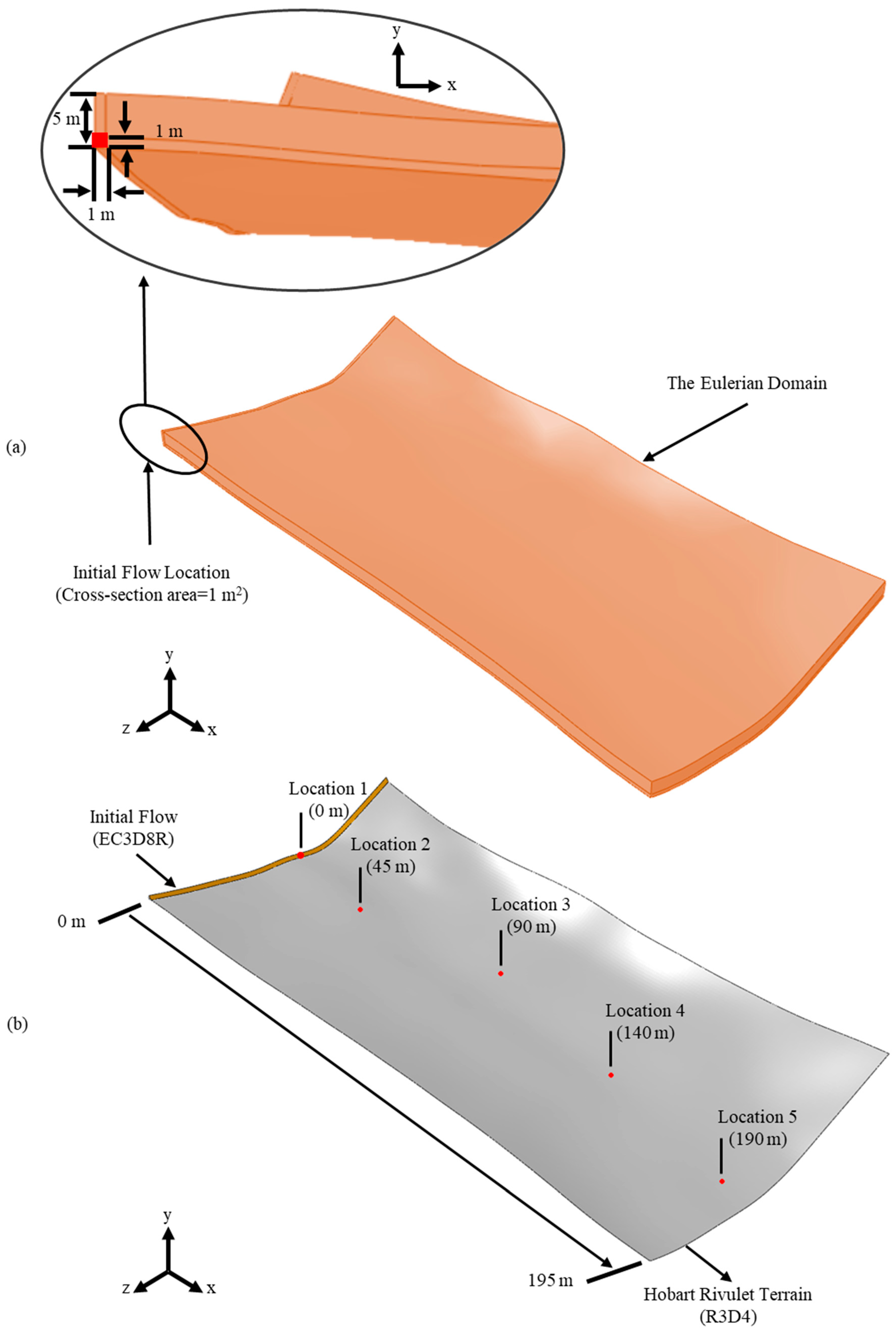
3.2.2. Simulation and Estimation

Focused on the study area described above, a 3D CEL model of the Hobart rivulet was established with the primary objective of estimating debris flow velocities at different locations along the flow path. This estimation serves as the initial component for the subsequent modelling of boulder–barrier interactions to investigate the effect of boulder velocity on structural performance. The simulation employed EC3D8R 8-node linear Eulerian brick elements with reduced integration and hourglass control to model the debris flow behaviour, utilising the Bingham visco-plastic material outlined in Section 2.2.

Table 1. Hobart rivulet model parameters [11].

Material Parameter	Constitutive Model	Density ρ (kg/m3)	$\mathbf{Yield} \mathbf{Stress} {\mathit{\tau }}_{\mathit{y}}$ (Pa)	$\mathbf{Viscosity} \mathit{\eta }$ (Pa·s)	Poisson’s Ratio ν	Young’s Modulus E (kPa)
Debris flow	Bingham	1500	100	100	-	-
Hobart Rivulet Terrain	Rigid body	-	-	-	-	-
Barrier *	Linear elastic	7850	-	-	0.25	2 $\times$ 108
Boulder *	Rigid body	2880	-	-	-	-

* Applied to the models in Section 3.3 and Section 4.

presents the essential parameters employed in the Hobart Rivulet model. The set-up of the Eulerian domain, initial debris flow, and the Hobart Rivulet terrain are referred to in Figure 4.

The initial debris flow, with a cross-sectional area of 1 m², was defined within the entire Eulerian domain, as illustrated in Figure 4a. Five locations set to measure the flow velocity are located at 0 m, 45 m, 90 m, 140 m, and 190 m away from the inlet in the X-direction, as shown in Figure 4b. Material parameters for the debris flow, as reported in the authors’ previous studies [11,27], were applied, while the terrain of the Hobart rivulet was simulated as rigid bodies using R3D4 4-node 3-D bilinear rigid quadrilateral elements. A contact penalty definition with a friction coefficient 0.15 was chosen for interactions between debris flow and the terrain. The model was subjected to a gravity load of 10 m/s², and a continuous initial flow velocity of 3 m/s was maintained throughout the 30-s simulation.

Figure 5 illustrates the time history of the debris flow velocity at five locations along the flow path, providing insights into the debris flow dynamics within the study area. At Location 1 (0 m), the velocity remains low and stable at 3 m/s due to the initial setting. Moving to Location 2 (45 m), a sharp spike in velocity occurs around the 5-s mark, reaching approximately 10 m/s before stabilising around 7 m/s. Similarly, at Location 3 (90 m), the velocity exhibits a sudden increase to approximately 18 m/s after 7 s, followed by stabilising around 12 m/s after some initial oscillations, showing that the debris flow continues to gain momentum. At Locations 4 (140 m) and 5 (190 m), the velocities exhibit more significant initial fluctuations, followed by stabilisation around 14 m/s and 16 m/s after approximately 25 s, respectively. The pronounced peaks and oscillations at these locations indicate a highly energetic and turbulent flow, likely influenced by changes in the terrain or flow conditions and cumulative momentum [53,54]. The observed stabilisation patterns at Locations 2 and 3 demonstrate a transition to a steady state, while the prolonged fluctuations at Locations 4 and 5 highlight more complex interactions and the energetic and turbulent nature of the downstream flow.

Based on these observations, a velocity of 12 m/s is utilised for subsequent investigations into modelling boulder–barrier interactions. Additionally, flow velocities of 3 m/s, 7 m/s, 12 m/s, 14 m/s, and 16 m/s, which are stabilised at each location, are employed to explore their effects on structural performance. Moreover, boulders are released at Location 3 at 25 s in benchmark simulations of flow–boulder–barrier interaction. Detailed information is provided in Section 3.3 and Section 4.

3.3. Simulation of Boulder–Barrier Interactions

To enhance the understanding of the effectiveness of an I-beam post barrier, an FE model of boulder–barrier interaction was developed. The simulation accounts for real-world scenarios based on on-site data gathered from Hobart Rivulet, taking into account the configuration of an existing I-beam post barrier. Following an on-site inspection, two types of beams, namely I- and C-beams, were used to model the existing debris mitigation systems surrounding Hobart Rivulet. The dimension of the I-beam employed in this study adheres to the standards outlined in AS-NZS 3679.1-2016 Structural steel Part 1: Hot-rolled bars and sections [55], with the classifications and specifications outlined in

Table 2. Specifications of beams used in the simulations [55].

Beam Type
Classification	UC200-59	150PFC
t1 (mm)	14.2	9.5
t2 (mm)	14.2	9.5
t3 (mm)	9.5	6
b1 (mm)	205	75
b2 (mm)	205	75
y (mm)	105	75
h (mm)	210	150

. Additionally, one type of I-beam post barrier that is currently constructed along the rivulet, as depicted in Figure 6a, was selected as a case study for the performance analysis. This barrier consists of 17 I-beam post and one flange installed on the top of the front row. The configuration and dimensions of the model are detailed in Figure 6b and

Table 3. Model configuration and dimensions of the I-beam barrier.

Post Beam Type	Flange Beam Type	s1 (m)	s2 (m)	s3 (m)	s4 (m)	s5 (m)	s6 (mm)	H * (m)
								Minimum	Maximum
UC200-59	150PFC	1.5	0.75	0.95	12.205	1.5	150	3.31	3.78

* The height of each I-beam post varies depending on the actual terrain; the maximum and minimum height of the post for the barrier are provided in this table only.

.

The FE model consists of two parts: one boulder and the I-beam post barrier. A feature of this model is the incorporation of elements capable of failure by introducing a damage characteristic of ductile steel beam sections, which simulates the vulnerabilities of the protective structure when subjected to boulder impacts, allowing for the identification of weak points of the protective system and investigating the factors that affect performance. Therefore, a key metric introduced is the failure ratio in assessing the efficacy of I-beam posts against boulder impacts. This ratio quantifies the proportion of elements within the barrier that fail during impact compared to the total number of elements present.

In the simulations, since the damping effects or deformation of the boulder are not of interest in this study, the boulder is modelled as a rigid body, while the steel I-beam barriers are considered linear elastic with ABAQUS Explicit type B31 2-node linear beam elements. In ABAQUS, these beam elements are conceptualised as one-dimensional entities operating within a three-dimensional space. Despite being simplified as 1D elements, ABAQUS allows for the detailed specification of cross-sectional properties, including parameters such as the area, moments of inertia, and shear stiffness. These settings enable the model to accurately account for bending moments and shear forces throughout the analysis. Additionally, these elements possess stiffness related to the deformation along the beam’s axis, while simultaneously allowing for transverse shear deformation between the axis and its cross-section directions. This dual capability categorises the beams employing such elements as shear flexible beams, capable of representing both bending and shear behaviours with high fidelity. The primary rationale for employing such beam elements in this study lies in their geometric simplicity and their suitability for scenarios involving contact and dynamic impact. Utilising these elements reduces the complexity of the model, thereby enhancing computational efficiency without compromising the accuracy of simulating physical phenomena [56]. A contact penalty definition with a friction coefficient of 0.15 has been adopted for the interaction between the boulder and the I-beam post. The model is subjected to a gravity load of 10 m/s², and each case is simulated for 0.5 s. The model setup involves a consideration of various parameters, including boulder location, velocity, size, impact height, and impact orientation. The details are provided and the results are discussed in the following sections.

3.3.1. Identifying the Weakest I-Beam Post of the Barrier

In the following simulations, the boulder is tilted at an angle of 45 degrees, and the distance between the centre of the boulder, the beam post, and the ground is 0.354 m. By impacting at a point on the I-beam surface, this setup aids in maximising the horizontal component of forces, distributing stress evenly, and simplifying computational calculations. Moreover, the boulder is set to move in the x direction with an initial speed of 12 m/s, while the barrier has a fixed base for each post, as described in Figure 7. In order to pinpoint the weakest post within the I-beam post barrier, the simulation is carried out systematically, with each I-beam post being individually subjected to boulder impacts. The test number corresponds to the beam number, as illustrated in Figure 6b.

Figure 8 compares the failure ratio and maximum impact force for two rows of I-beam posts in the barrier: the front row (FN series) and the back row (BN series). In the upper plot of this figure, the FN series (Tests FN1 to FN9) shows failure ratios ranging from 3.6% to 4.8% and maximum impact forces ranging from 170 kN to 180 kN. Test FN3 has the highest maximum impact force at 180 kN, while Test FN9 has the highest failure ratio at 4.8%. The differences between the maximum and minimum values are approximately 5% for impact force and 24% for failure ratio. This suggests there is no significant difference in impact forces among the posts, but there is a considerable difference in failure ratios. Similarly, the lower plot for the BN series (Tests BN1 to BN8) shows failure ratios from 3.4% to 4.8% and maximum impact forces from 168 kN to 176 kN. Test BN3 has the highest failure ratio at 4.8%, with a 30% difference from the minimum, while Test BN7 has the highest maximum impact force at 176 kN, with a 4% difference from the minimum. These findings indicate that the failure ratio appears to be a highly effective metric for evaluating damage to the entire barrier. Accordingly, FN9 and BN3 are the weakest posts in their respective rows due to their highest failure ratios. However, since boulders are more likely to impact the front row of the barrier first, FN9 can be considered the weakest post of the entire barrier, which will be the focus of subsequent investigations.

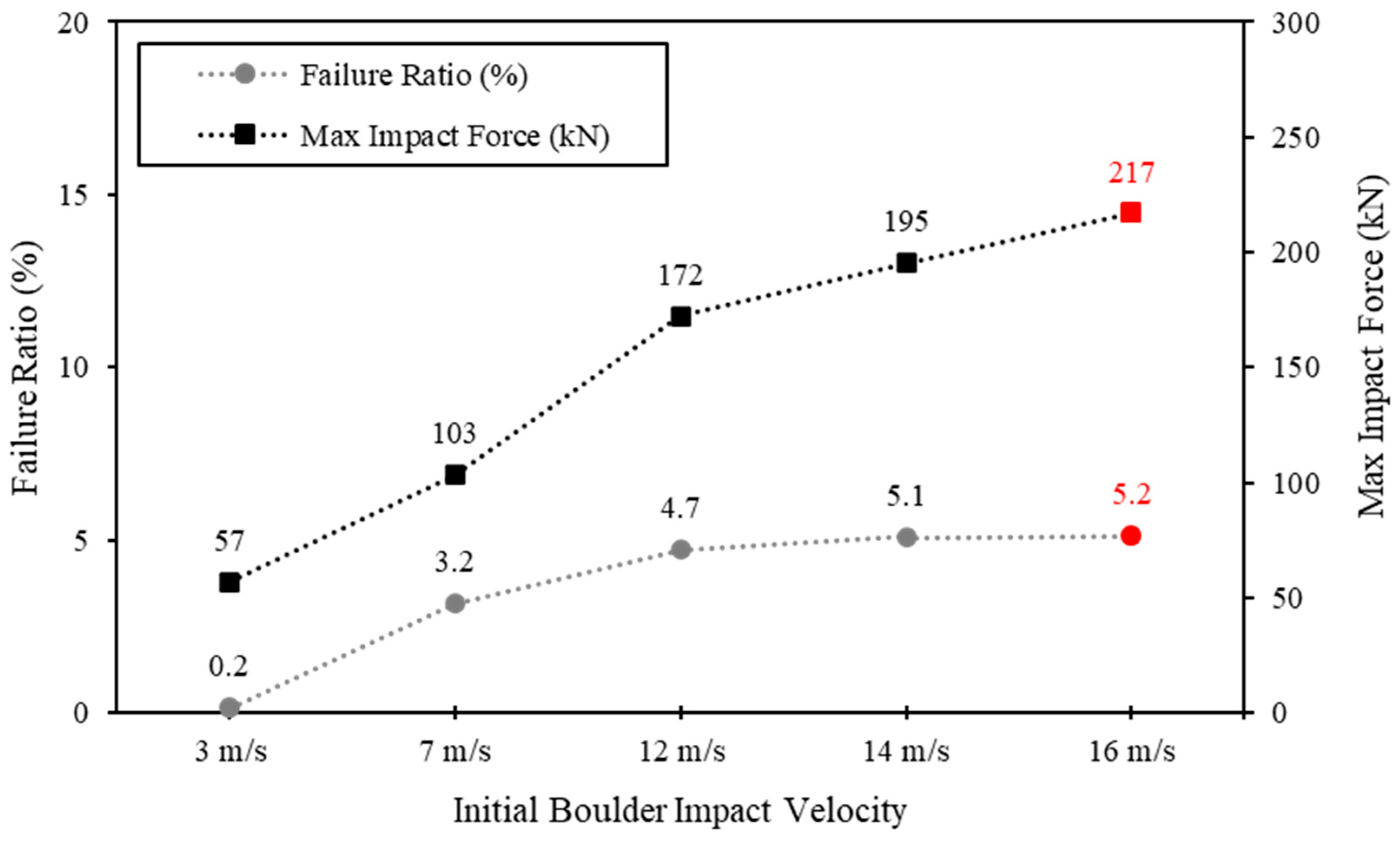
3.3.2. Effect of Boulder Impact Velocity

Various initial velocities are applied to the boulder impacting the FN9 I-beam post, as depicted in Figure 9. Based on the investigation in Section 3.2, five cases are examined, with the initial boulder velocities ranging from 3 m/s to 16 m/s. Figure 10 presents a comparative analysis of the failure ratio and maximum impact force experienced by the FN9 I-beam post. At a lower velocity of 3 m/s, the failure ratio is minimal at 0.2%, and the impact force is relatively low at 57 kN. However, as the velocity increases to 7 m/s, the failure ratio grows to 3.2%, with the impact force nearly doubling to 103 kN. This indicates significant structural damage and higher forces. The trend continues with further increases in velocity, with the failure ratio reaching 4.7% and the impact force rising to 172 kN at 12 m/s, and 5.1% and 195 kN at 14 m/s, respectively. Notably, at 16 m/s, while the failure ratio only slightly increases to 5.2%, the impact force peaks at 217 kN.

The linear increase in maximum impact force with velocity is due to the kinetic energy transfer, indicating that higher velocities result in exponentially greater kinetic energy, translating to increased impact forces. The plateauing of the failure ratio at higher velocities suggests a potential threshold where the material properties or design limits of the barrier are reached, stabilising the failure ratio but allowing force to continue escalating. As expected, the stabilised failure ratio suggests that out of the 17 I-beam posts in the barrier, the one struck by the boulder is completely damaged. At lower velocities, the I-beam post can effectively absorb the energy without sustaining significant damage, resulting in a low failure ratio. However, as the velocity increases to a certain point, the capacity of the post to absorb and distribute impact energy becomes saturated. This saturation causes the material to enter a stage of plastic deformation, where it absorbs energy through permanent deformation rather than increasing the failure ratio. Consequently, the failure ratio stabilises even as the impact force continues to increase. These findings indicate a strong correlation between increasing boulder impact velocity and both the failure ratio and maximum impact force. The impact velocity needs to be considered carefully in designing and assessing I-beam barriers, as even small increases in velocity at higher ranges can result in significantly greater forces and potential structural damage.

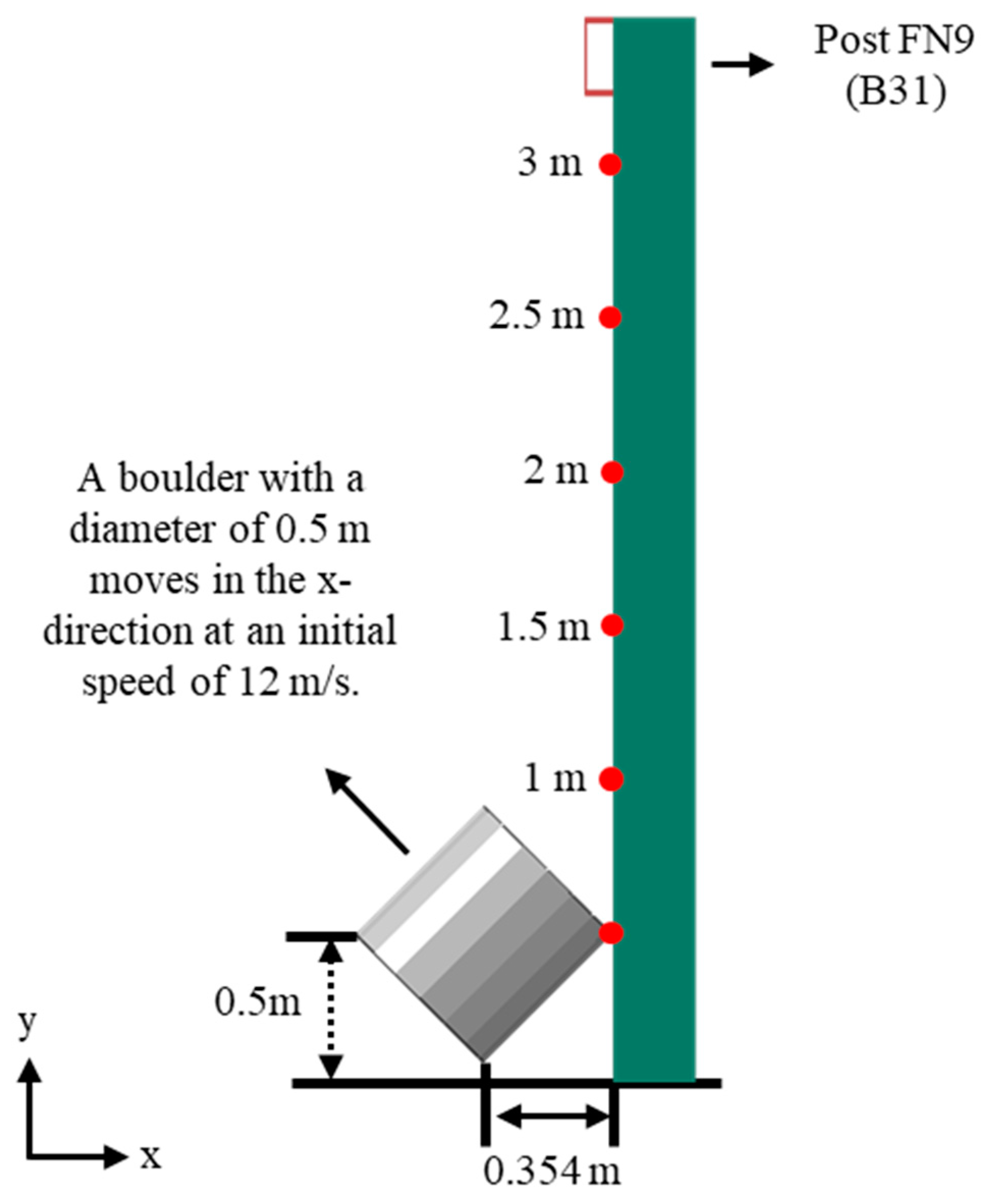
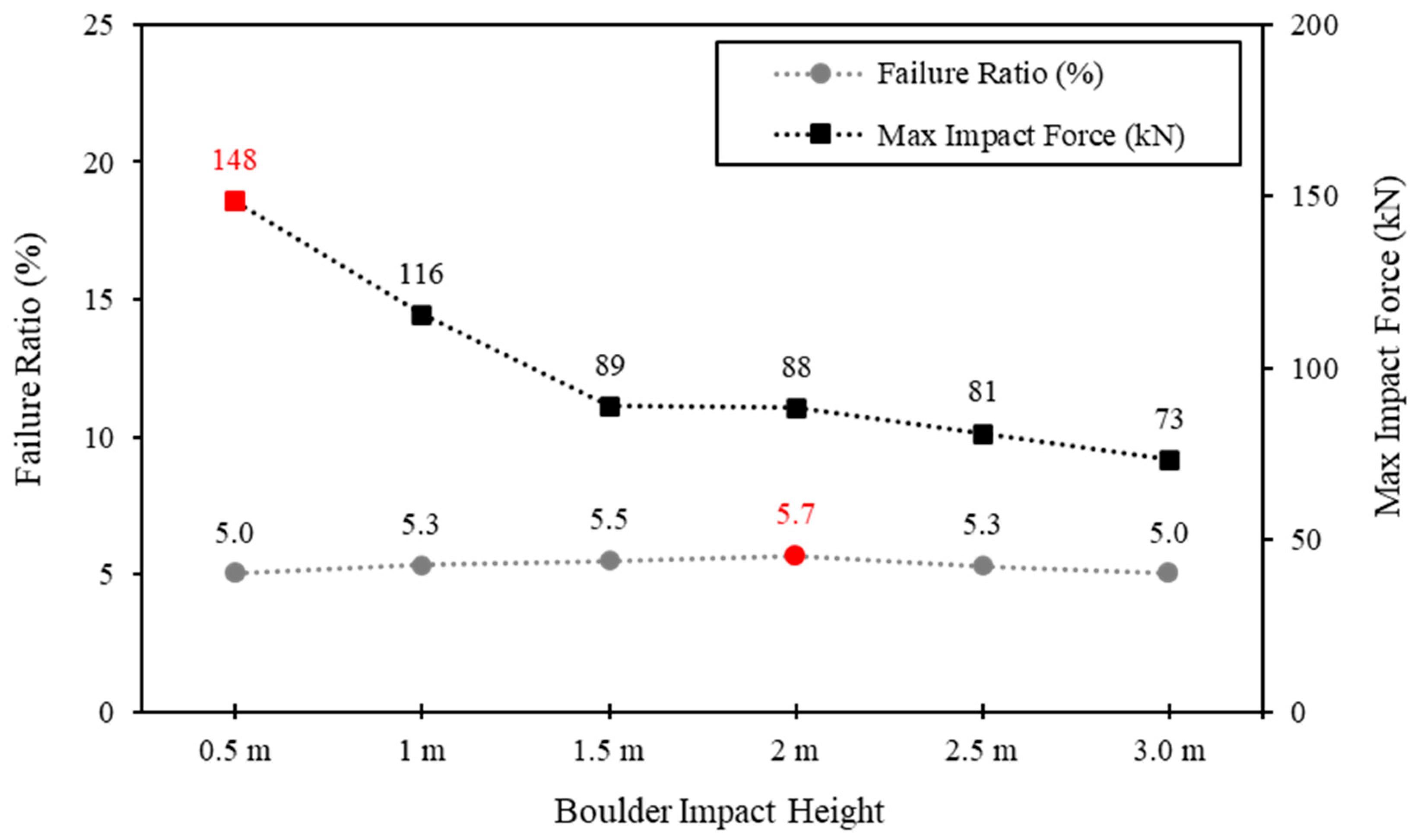
3.3.3. Effect of Boulder Impact Height

The impact of a boulder with a diameter of 0.5 m and an initial speed of 12 m/s is examined, placed at various heights ranging from 0.5 m to 3 m, as illustrated in Figure 11.

From Figure 12, at the lowest impact height of 0.5 m, the failure ratio is 5.0%, and the maximum impact force is the highest at 148 kN among all cases. This high impact force suggests that the energy imparted by the boulder is highly concentrated at a low height, leading to significant force transmission and potential structural damage. As the impact height increases to 1.0 m, the failure ratio slightly rises to 5.3%, but the maximum impact force decreases to 116 kN. This trend of decreasing maximum impact force continues with further increases in height, peaking in a failure ratio of 5.7% at 2.0 m. When the height increases to 2.5 m and 3.0 m, the failure ratio decreases to 5.3% and 5.0%, respectively, and the maximum impact force decreases to 81 kN at 2.5 m and 73 kN at 3.0 m. This decline in both metrics indicates that higher impact heights lead to a more significant reduction in both structural damage and force transmission.

Overall, as the impact height increases, the maximum impact force decreases while the failure ratio initially increases, peaking at 2.0 m before declining. Notably, in this study, the middle of the I-beam post exhibits higher failure ratios than the upper or lower parts, suggesting that optimising these mid-sections can limit damage and enhance structural resilience against dynamic loads.

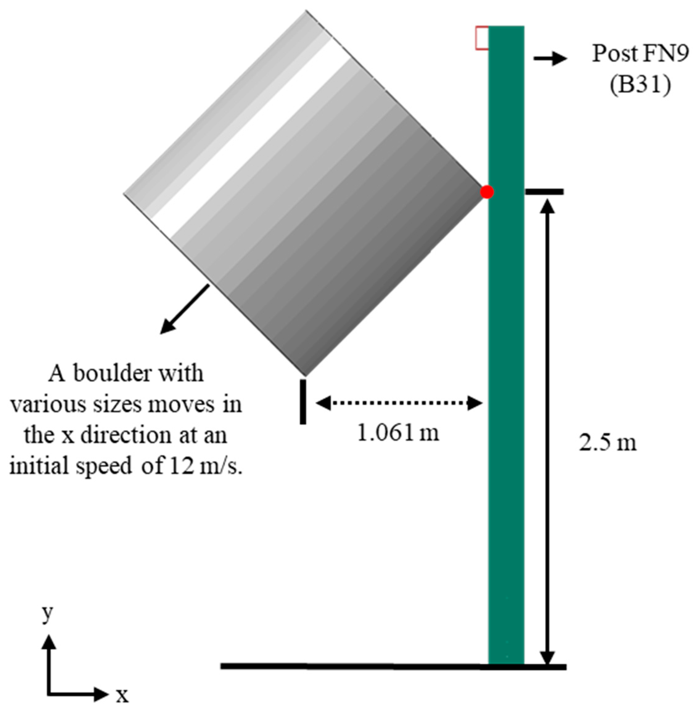
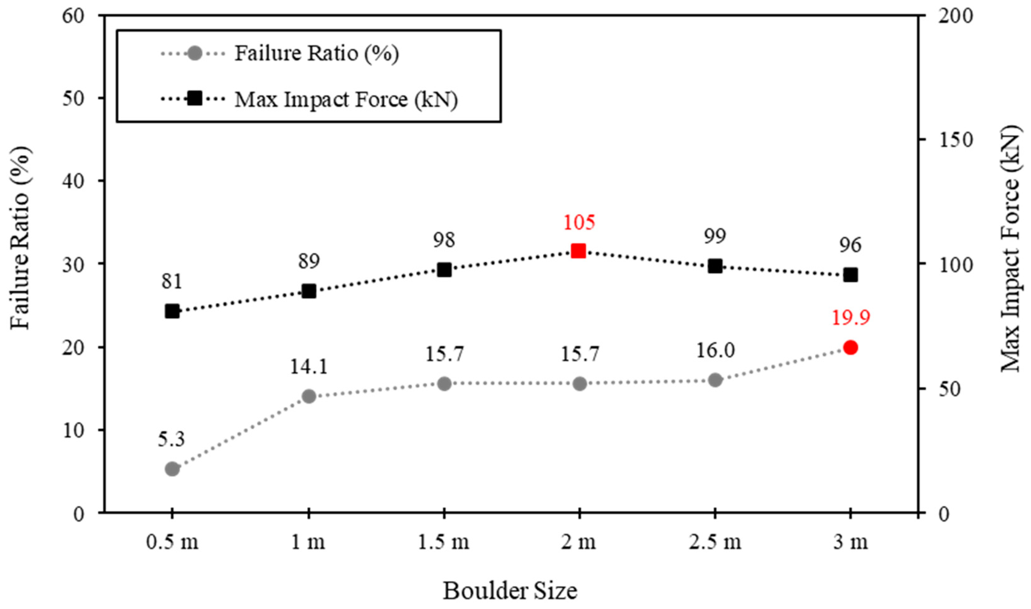
3.3.4. Effect of Boulder Size

To investigate the effect of boulder size, simulations are conducted using cylindrical boulders in six different sizes: 0.5 m, 1 m, 1.5 m, 2 m, 2.5 m, and 3 m. Based on previous findings, the boulder is placed in front of the weakest I-beam post (FN9) at a height of 2.5 m. Using the case S3, an example of the model configuration is shown in Figure 13. Moreover, a reference size (S_R) was used to standardise boulder sizes.

Table 4. Boulder geometries.

Geometry	Test No	Reference Size SR (m)	Volume (m3)	Mass (tons)
	S1	0.5	0.1	0.3
	S2	1	0.8	2.3
	S3	1.5	2.7	7.6
	S4	2	6.3	18.1
	S5	2.5	12.3	35.3
	S6	3	21.2	61.1

provides the properties of these boulders, detailing their size, volume, and other relevant parameters.

Figure 14 compares the failure ratio and maximum impact force on I-beam columns when impacted by boulders of different sizes. Starting with the smallest boulder size of 0.5 m, the failure ratio stands at 5.3%, accompanied by a maximum impact force of 81 kN. As the boulder size increases, there is a notable increase in the failure ratio, reaching 14.1% at a boulder size of 1 m. However, for boulder sizes ranging from 1.5 m to 3 m, the increase in failure ratio is marginal, with values ranging from 15.7% to 19.9%. Concurrently, the impact force exhibits a slight uptick across these sizes, peaking at 105 kN for a boulder size of 2 m. These results indicate that smaller boulders result in lower failure ratios, while larger boulders (2.5 m to 3.0 m) increase the failure ratio but reduce the peak impact force.

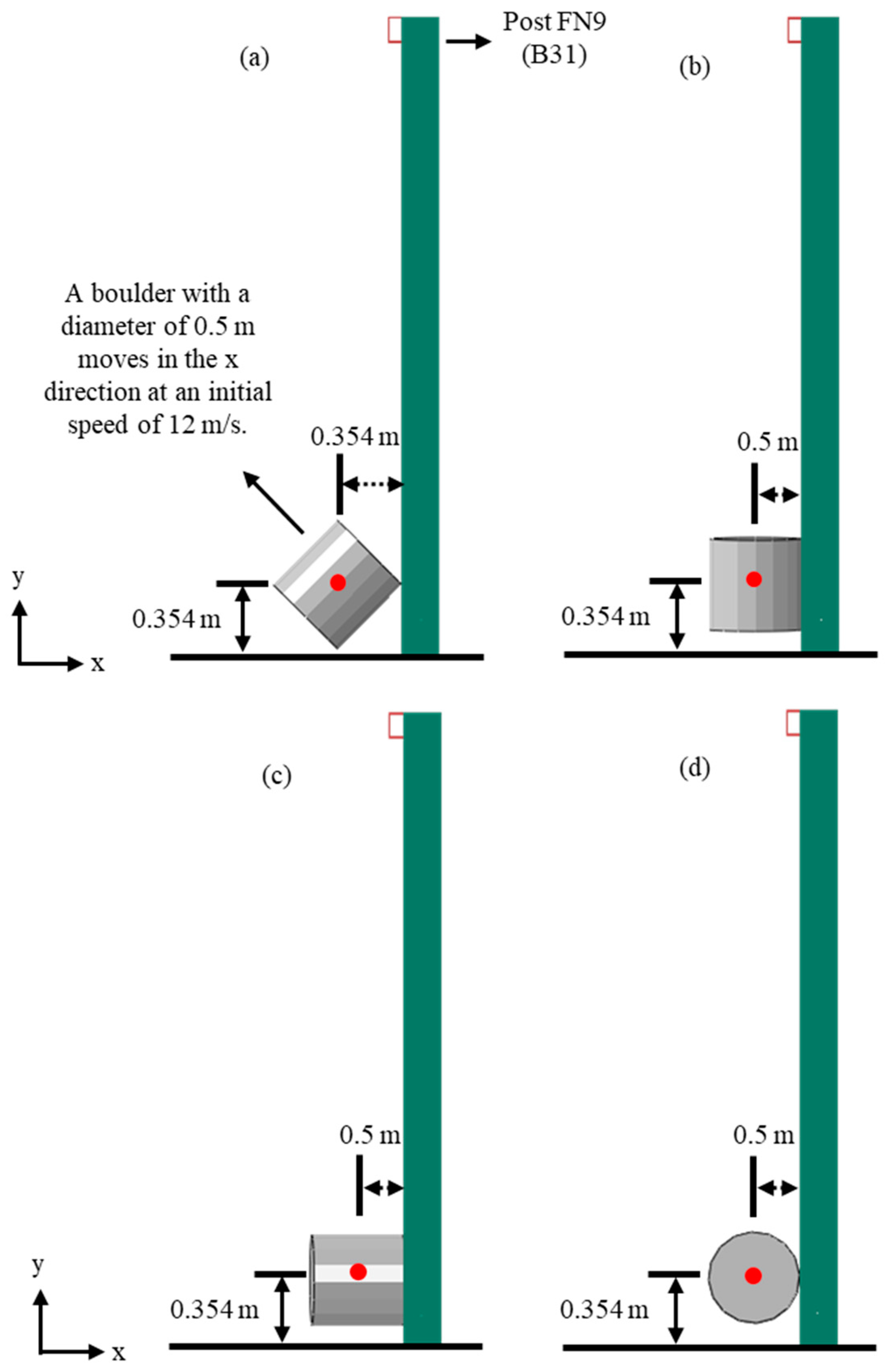
3.3.5. Effect of Boulder Orientation

Figure 15 shows the models of boulder–structure interaction used to investigate the effect of boulder orientation. These orientations include interactions with the boulder’s circular surface: (a) at a 45-degree inclination; (b) at 90 degrees to the Y-axis; (c) at 90 degrees to the X-axis; (d) at 90 degrees to the Z-axis. In each test, the boulder is placed at a height of 0.354 m in front of the FN9 I-beam post. The distance between the centre of the boulder and the post varies depending on the impact orientation.

The simulation results are presented in Figure 16. For impact orientation (a), the failure ratio is 4.7%, with a maximum impact force of 172 kN. Impact orientations (b) and (c) exhibit slight increases in both failure ratio and maximum impact force compared to orientation (a). Specifically, impact orientation (b) has a failure ratio of 5.1%, the highest among the orientations, and impact orientation (c) exhibits the highest maximum impact force at 182 kN. In contrast, impact orientation (d) shows a lower maximum impact force but a marginal increase in failure ratio.

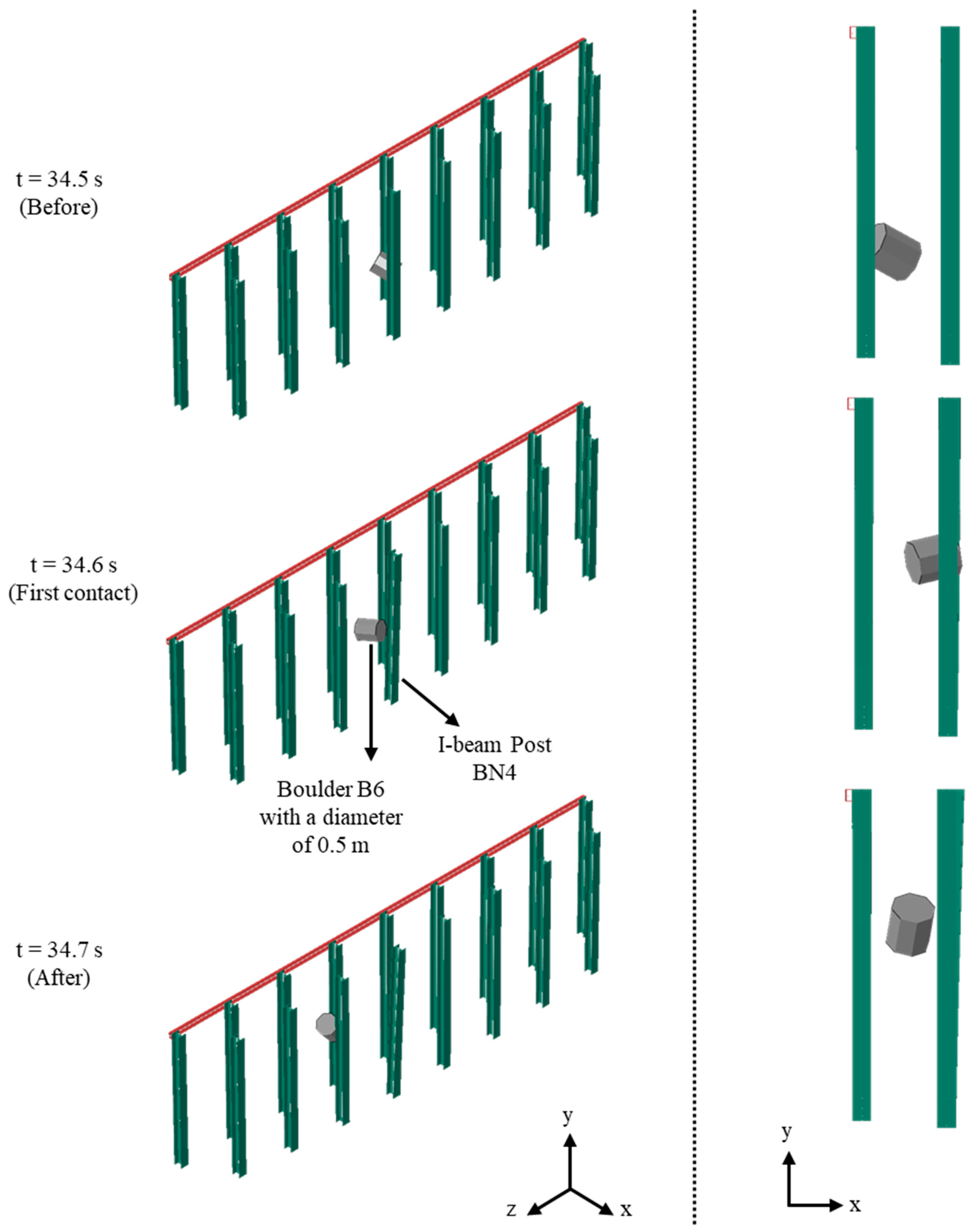
4. Benchmark Simulations of Flow–Boulder–Barrier Interactions

4.1. Parameters and Simulations

A CEL model is used to explore how the selected I-beam barrier interacts with boulders transported by debris flow within the study area. Within this model, the debris flow is represented by the fluid component and is meshed using the Eulerian continuum three-dimensional elements. The solid elements, such as the rivulet terrain, boulders, the funnel with a lid, and the barrier, are represented using Lagrangian discretisation. The configuration and material parameters for the flow–boulder–barrier interaction applications are provided in Figure 17 and Table 1 and Table 4, respectively. As discussed in Section 2.2 and Section 3.2, the debris flow is modelled using the Bingham visco-plastic material with EC3D8R 8-node linear Eulerian brick elements. To simulate both the boulders and the I-beam post barrier, according to Section 3.3, ABAQUS Explicit type R3D4 4-node 3-D bilinear rigid quadrilateral elements are employed to model boulders, while ABAQUS Explicit type B31 2-node linear beam elements are applied to the I-beam post barrier.

To incorporate boulders into the Bingham fluid, a funnel with a square lid is placed 5 m above the ground and 95 m from the I-beam post barrier. As determined in Section 3.3, the optimal timing for releasing boulders into the debris is based on the observation that the flow velocity stabilises at approximately 12 m/s after 20 s at this location. Therefore, the lid is removed at 25 s to ensure the flow reaches a steady state beneath the funnel. To prevent boulder entrapment and unrealistic kinetic energy generation during descent, the funnel vibrates at 0.2 Hz in the Y-direction and 0.03 Hz in the Z-axis. Ten boulders, labelled from B1 to B10, are initially positioned above the lid and dropped randomly onto the funnel as the simulation begins. A contact penalty definition with a friction coefficient of 0.15 is defined for interactions between boulders, debris flow, barrier, and the terrain. The model is subjected to a gravity load of 10 m/s², and a continuous initial flow velocity of 3 m/s was maintained throughout the 50-s simulation. To evaluate the performance of such a barrier, three simulations were conducted using boulder sizes of 0.5 m, 1.5 m, and 2.5 m, referring to Cases C1, C2, and C3, respectively. For a comprehensive understanding of the model configuration, refer to the detailed description provided by Sha et al. [27].

4.2. Results, Analysis, and Comparison

To assess the efficacy of the I-beam post barrier against the impacts of various sizes of boulders, Figure 18 offers a comparison of the failure ratio due to boulder impacts on the entire barrier at the simulation time 50 s. Since the size of the boulders varies in each case, the movement mechanisms, trajectories, and arrival time of the boulders during their transport in the debris flow also vary. At 50 s, the failure ratio of each case is stabilised at approximately 4%, 68%, and 89% in response to the boulder size of 0.5 m, 1.5 m, and 2.5 m, respectively, as expected, suggesting larger boulders lead to more significant damage of the barrier. Specifically, these failure ratios correspond to 1, 12, and 16 fully failed I-beam posts in the barrier. Figure 19 visualises the number of fully failed I-beam posts at both 0 s and 50 s, clearly showing how the failure ratios translate to the actual damage in each case. This demonstrates the capability of the CEL method in simulating the intricate interaction between the flow, boulders, and the I-beam post barrier to evaluate the structural performance for debris mitigation.

Focusing on the first boulder that reached the barrier location, Figure 20, Figure 21 and Figure 22 illustrate the collision between the boulder and the corresponding I-beam post of the barrier, capturing the moments before, during, and after the initial impact for 0.2 s. Using Case C2 as an example, with a boulder diameter of 1.5 m, boulder B6 arrives in front of I-beam post FN9 at 34.4 s. At 34.5 s, the boulder makes initial contact with the FN9 post, causing the I-beam to start deforming and leading to structural failure. By 34.6 s, the boulder continues moving, resulting in increased deformation and a higher failure ratio.

Figure 23 provides a comparative analysis of the failure ratio, impact force, and boulder velocity for three cases (C1, C2, and C3) before, during, and after the boulder’s collision with the barrier. In Figure 23a, all cases begin with a failure ratio of 0%. Upon first contact, the failure ratios increase to 3.3%, 7.1%, and 13.6% for C1, C2, and C3, respectively. Following the initial collision, the failure ratio continues to rise sharply to 38.6% for C3, 14.2% for C2, and remains at 3.3% for C1, demonstrating that larger boulders cause significantly more damage to the barrier. From Figure 23b, it is evident that all cases have an impact force of 0 kN before the collision. Upon first contact, the impact forces are 11 kN for C1, 26 kN for C2, and 33 kN for C3. These forces continue to increase substantially, reaching 24 kN for C1, 83 kN for C2, and 120 kN for C3. This pattern indicates that larger boulders exert significantly higher impact forces on the barrier, correlating with the higher failure ratios observed. Figure 23c shows the boulder velocities at 10.5 m/s for C1, 12.9 m/s for C2, and 13.0 m/s for C3 before the collision. During initial contact, the velocity for C1 drops sharply to −2.4 m/s, indicating a bounce-back or recoil effect, while the velocities for C2 and C3 reduce slightly to 12.2 m/s and 12.5 m/s, respectively. After the collision, the velocity for C1 remains negative at −2.3 m/s, showing continued recoil, whereas the velocities for C2 and C3 drop to 8.9 m/s and 9.8 m/s, respectively, indicating significant deceleration post-impact but no recoil.

Due to the complexity of flow–boulder–barrier interactions on the real Hobart Rivulet terrain, it is important to note that boulders of varying sizes exhibit different heights, velocities, and impact modes when colliding with different I-beam posts. To further explore the boulder–barrier interactions discussed in Section 3.3, three simplified FE models are established using observations from the CEL models for the three cases mentioned above. These FE models are designed to facilitate a comparative evaluation of their performance and effectiveness. Figure 24 provides the configurations of these FE boulder–barrier interaction models derived from CEL model observations, including impact height, velocity, and mode.

Figure 25 presents a comparative analysis of the performance of the CEL and FE models across three impact scenarios (D1, D2, and D3, corresponding to the first boulder impact orientations from C1, C2, and C3) based on the failure ratio, impact force, and boulder velocity after the initial impact. Figure 25a compares the failure ratio between the two approaches under the impact of the boulder. For D1, the CEL model shows a failure ratio of 3.3%, while the FE model shows a slightly higher ratio at 4.0%. As the boulder size increases in D2, both models present similar failure ratios, with the CEL model at 14.2% and the FE model at 14.3%. For the largest boulder size in D3, the failure ratio significantly increases, with the CEL model at 38.6% and the FE model slightly lower at 33.9%. The higher failure ratio observed in the CEL model for this scenario can be attributed to its detailed representation of large deformations and fluid–solid–structure interactions, which are more pronounced with larger boulders. The sensitivity of the CEL model to these complex dynamics likely results in a higher and more realistic prediction of failure, whereas the FE model might not capture these intricacies as effectively, leading to a slightly lower failure ratio. In Figure 25b, the CEL model predicts an impact force of 24 kN, while the FE model estimates a higher force of 31 kN in D1. For D2, the impact forces are 83 kN for the CEL model and 85 kN for the FE model, showing close agreement. For D3, the impact forces rise substantially, with the CEL model at 120 kN and the FE model significantly higher at 163 kN. Regarding boulder velocity as shown in Figure 25c, the CEL model shows a negative velocity of −2.3 m/s for D1, indicating a rebound or change in direction, whereas the FE model shows a near-zero velocity of −0.1 m/s. For D2 and D3, the velocities are close, with the CEL model at 8.9 m/s and 9.8 m/s, and the FE model slightly higher at 9.4 m/s and 10.7 m/s, respectively.

Figure 26 further compares the percent difference between CEL and FE models for failure ratio, impact force, and boulder velocity across these three scenarios. The results show that the models are highly comparable for failure ratio, with differences ranging from 0.6% to 22.7%. However, for impact force and boulder velocity, the differences are substantial and inconsistent, with impact force differences ranging from 1.8% to 36.7% and boulder velocity differences ranging from 5.8% to 95.3%.

Figure 27 compares the visualisation of failed elements of the barrier at 0.2 s after the first boulder impact between these two approaches. Each visualisation depicts the barrier state under three impact scenarios, with non-failed elements in blue and failed elements in grey. For S_R = 0.5 m (D1), both approaches show minimal failures, indicating that the barrier withstands small impacts effectively. At S_R = 1.5 m (D2), the CEL model reveals concentrated failures, particularly in the middle and upper sections, while the FE model shows a more dispersed failure pattern. For S_R = 1.5 m (D3), both methods indicate extensive barrier failure, although the failure distribution varies slightly, with CEL showing more concentrated damage.

Overall, based on these comparisons, both approaches are broadly comparable in assessing whether the barrier fails under various impacts but offer different insights into specific structural weaknesses. This complementarity is crucial for the design and performance assessment of such protective barriers, especially when there is a need to optimise the structure or compare the performance of multiple barriers. However, this study is not without limitations, primarily due to the simplifications inherent in the FE models. These models, although effective for preliminary assessments, may not capture all the complexities of real-world boulder–barrier interactions observed on the Hobart Rivulet terrain. Variations in boulder shape, material properties, and nuanced interactions between boulders and I-beam posts are simplified to make the models computationally feasible. This could lead to discrepancies between the FE model predictions and actual field behaviour, potentially affecting the accuracy of the failure ratio, impact force, and boulder velocity estimations. Additionally, using a fixed set of impact scenarios may not encompass the full range of possible real-world conditions, limiting the generalisability of the findings. These limitations might have influenced the outcomes and interpretations, leading to under- or over-estimations of barrier performance under different impact scenarios. To address these issues, it is recommended that more detailed real-world data be integrated into the models to better capture the complexities of boulder–barrier interactions in future research, including adjusting assumptions about boulder shape, velocity, and location to accurately reflect regional conditions. Additionally, conducting extensive field tests to validate and calibrate the models would enhance their accuracy and reliability. Combining the strengths of both CEL and FE models can offer a more comprehensive evaluation. Therefore, a simplified FE model can be used to perform a preliminary failure assessment; meanwhile, the CEL model can be used to investigate the barrier performance fully and guide decisions on strengthening specific areas to improve structural designs.

5. Conclusions

This study addresses challenges in evaluating the effectiveness and reliability of protective structures for debris flow risk mitigation. By incorporating numerical modelling, the study proposes a procedure to assess the performance of protective structures, focusing on flow–boulder–barrier interactions using the CEL method. Building on previous research on boulders transported by debris flow in an Australian rivulet, the study examines an existing I-beam post barrier along the Hobart Rivulet as a real-world case. The following conclusions are drawn:

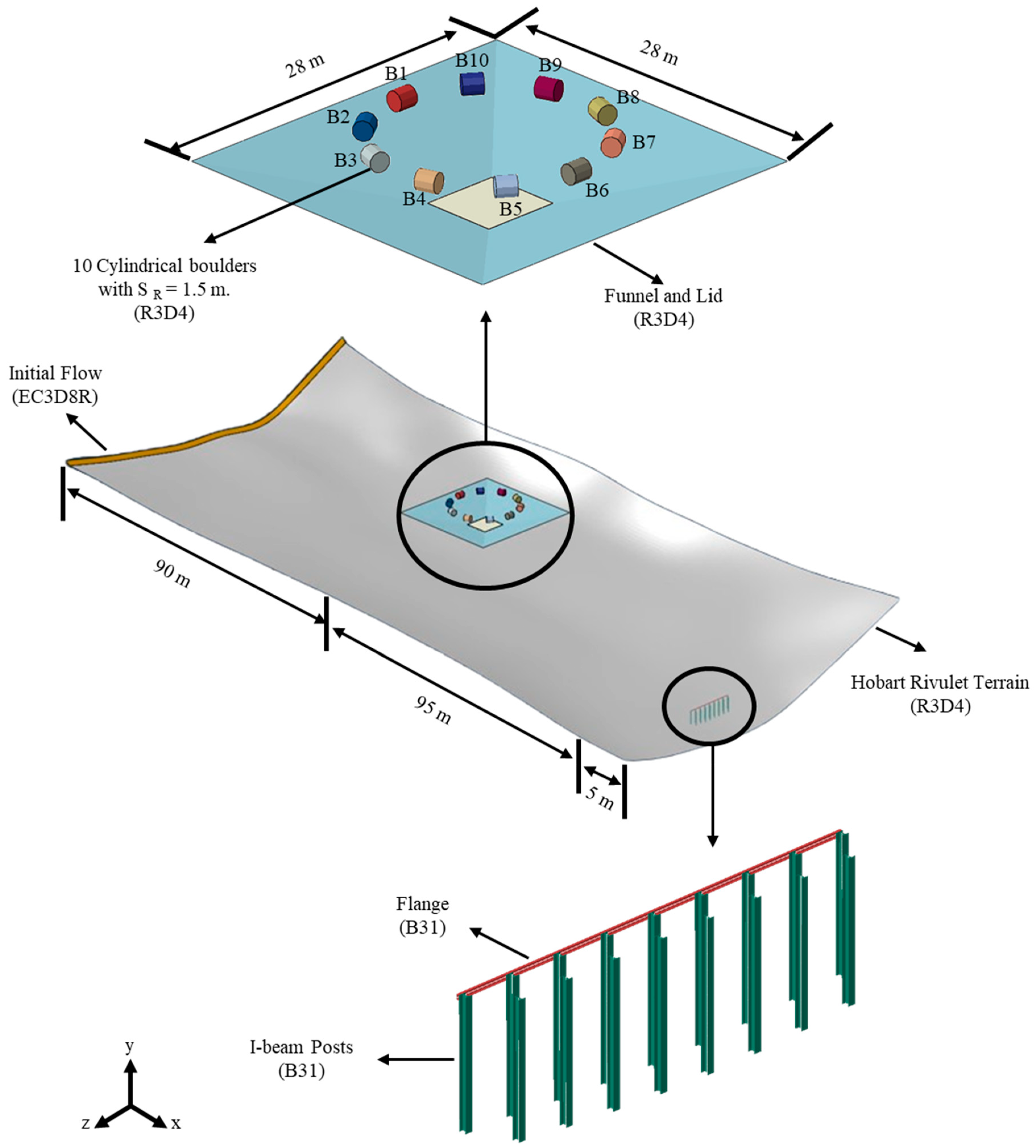
• The CEL model is validated by simulating experimental debris flow tests from Ng et al. [52] using the Bingham model. The good agreement between the CEL model and experimental data suggests accurate predictions of flow velocities, boulder velocities, and impact forces. Subsequent examinations of debris flow velocities along the Hobart Rivulet using a 3D CEL model reveal distinct flow dynamics. Beginning at 3 m/s, flow velocities surged downstream, stabilising at 7 m/s, 12 m/s, 14 m/s, and 16 m/s, indicating increasing momentum and turbulence downstream. These findings provide a foundation for subsequent investigations into boulder-barrier interactions, with a designated velocity of 12 m/s used for the structural effect analysis in Section 3.3, and the release of boulders at a specific location for benchmark simulation in Section 4.
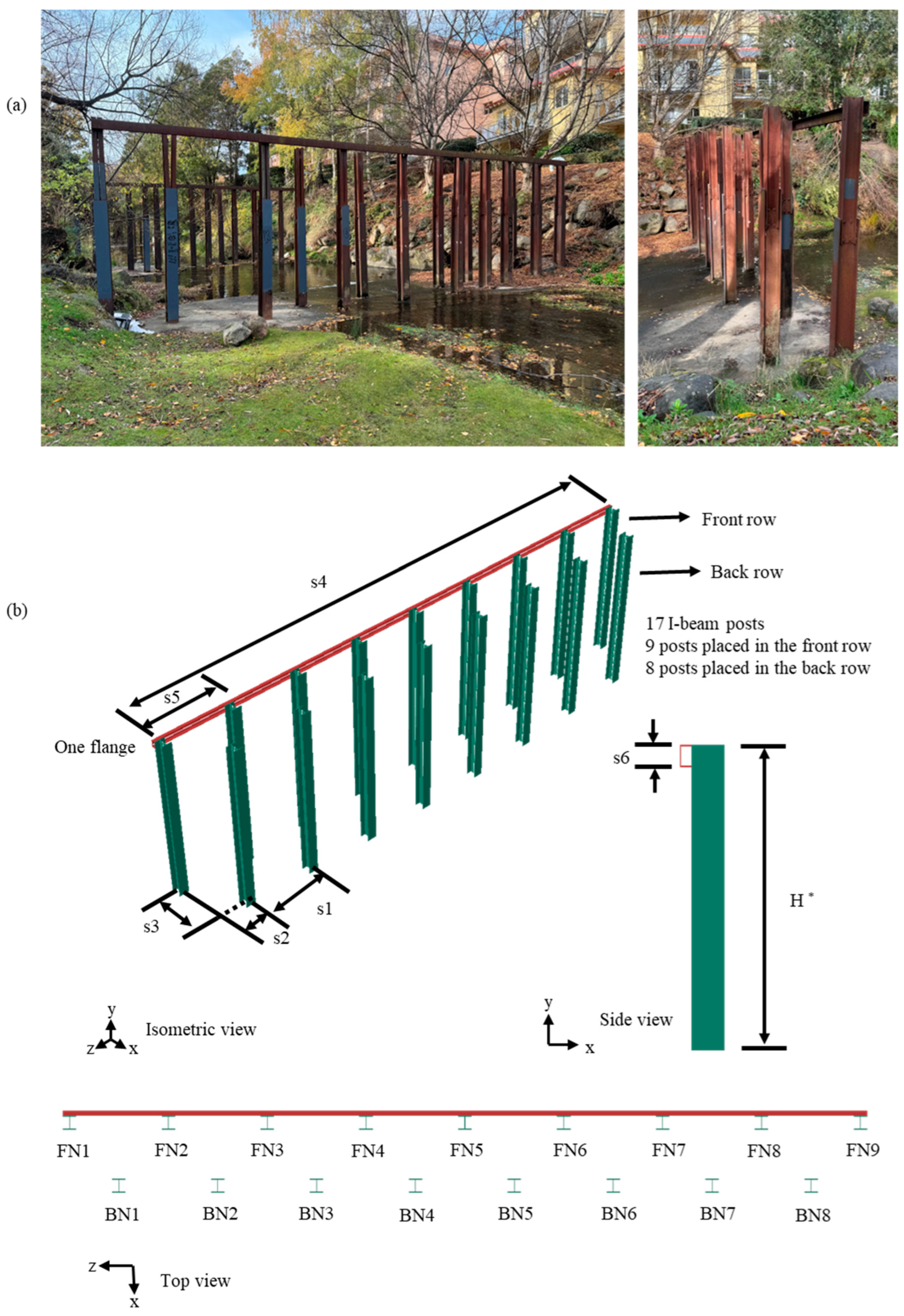
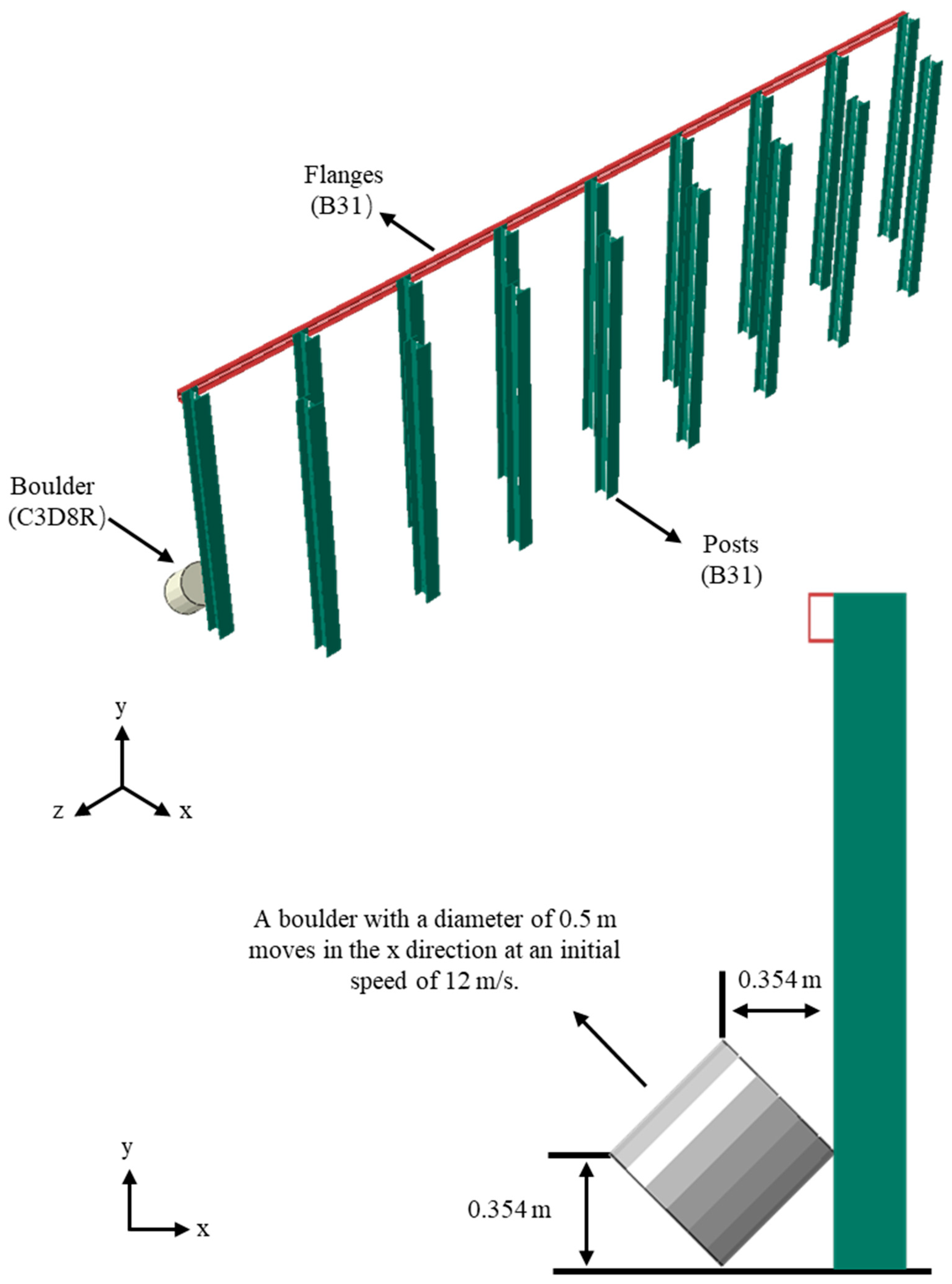
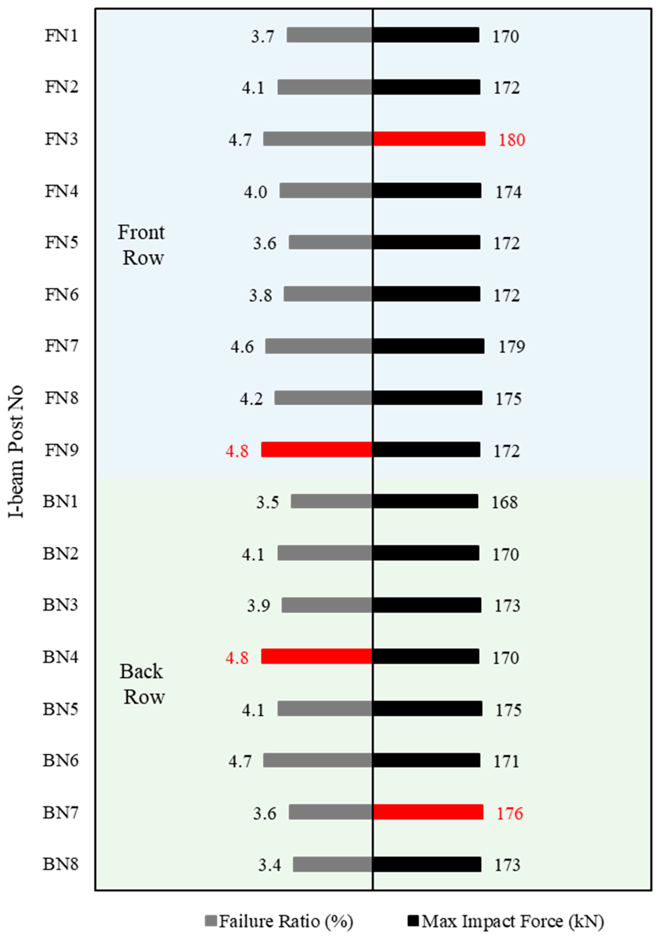
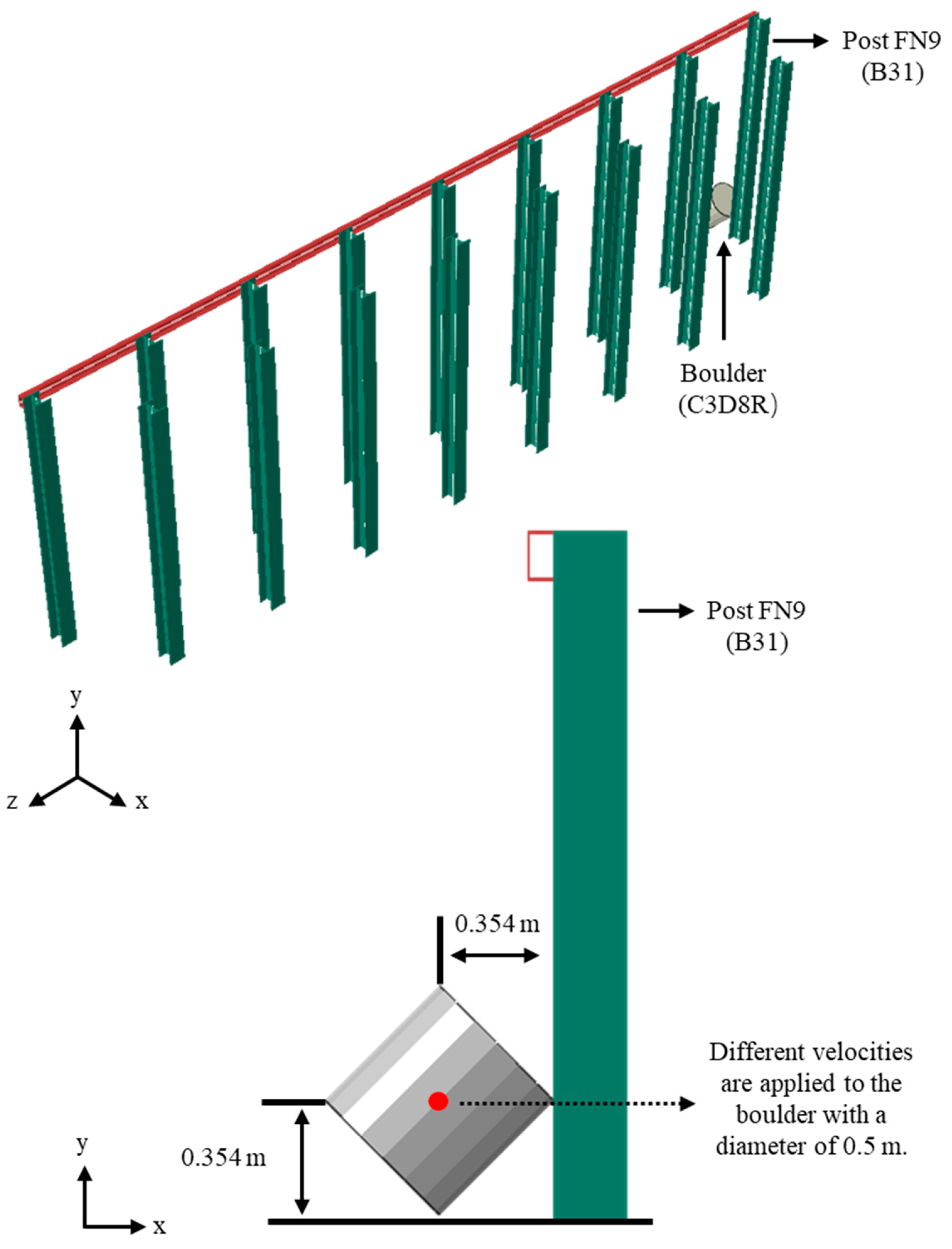
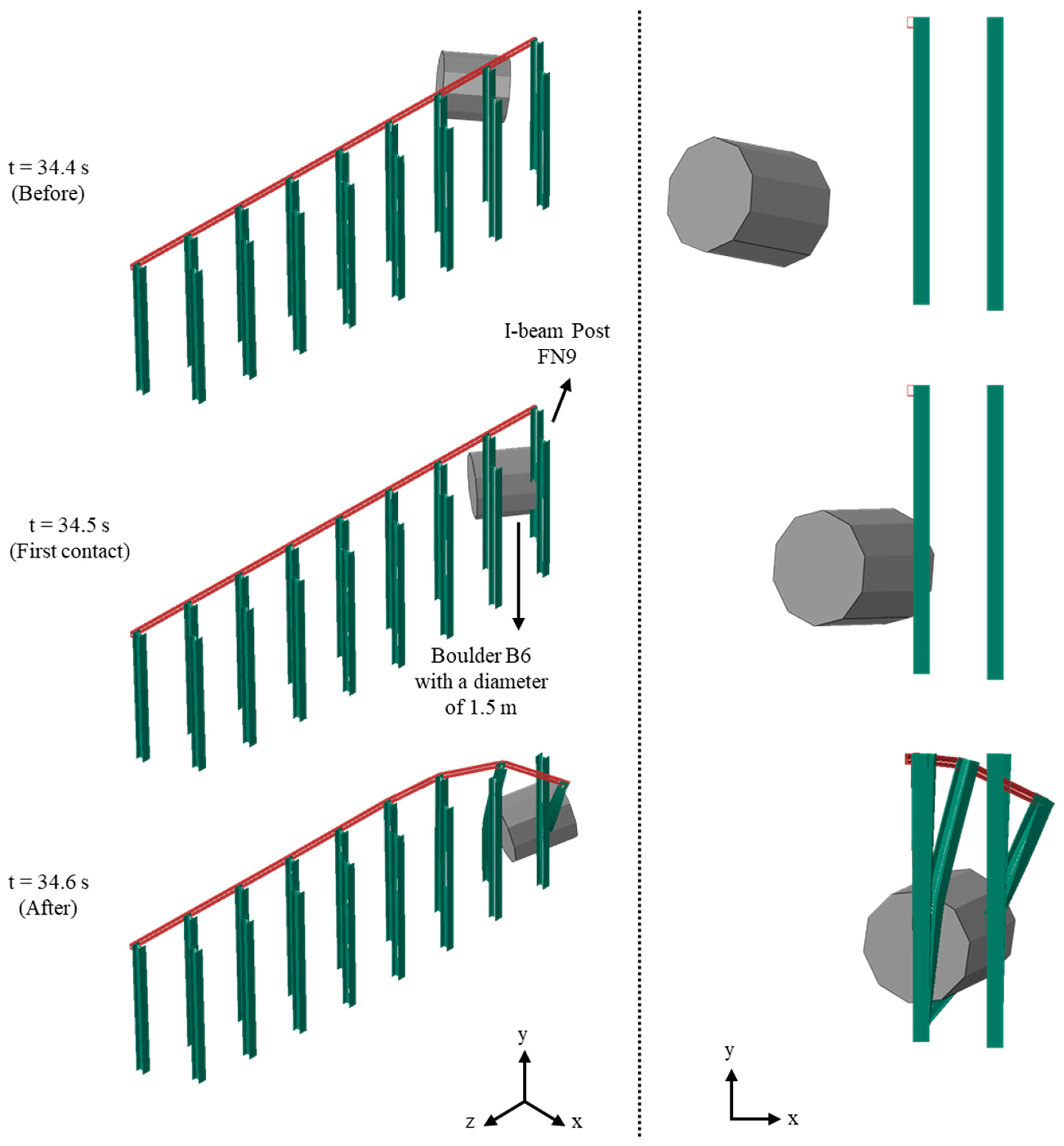
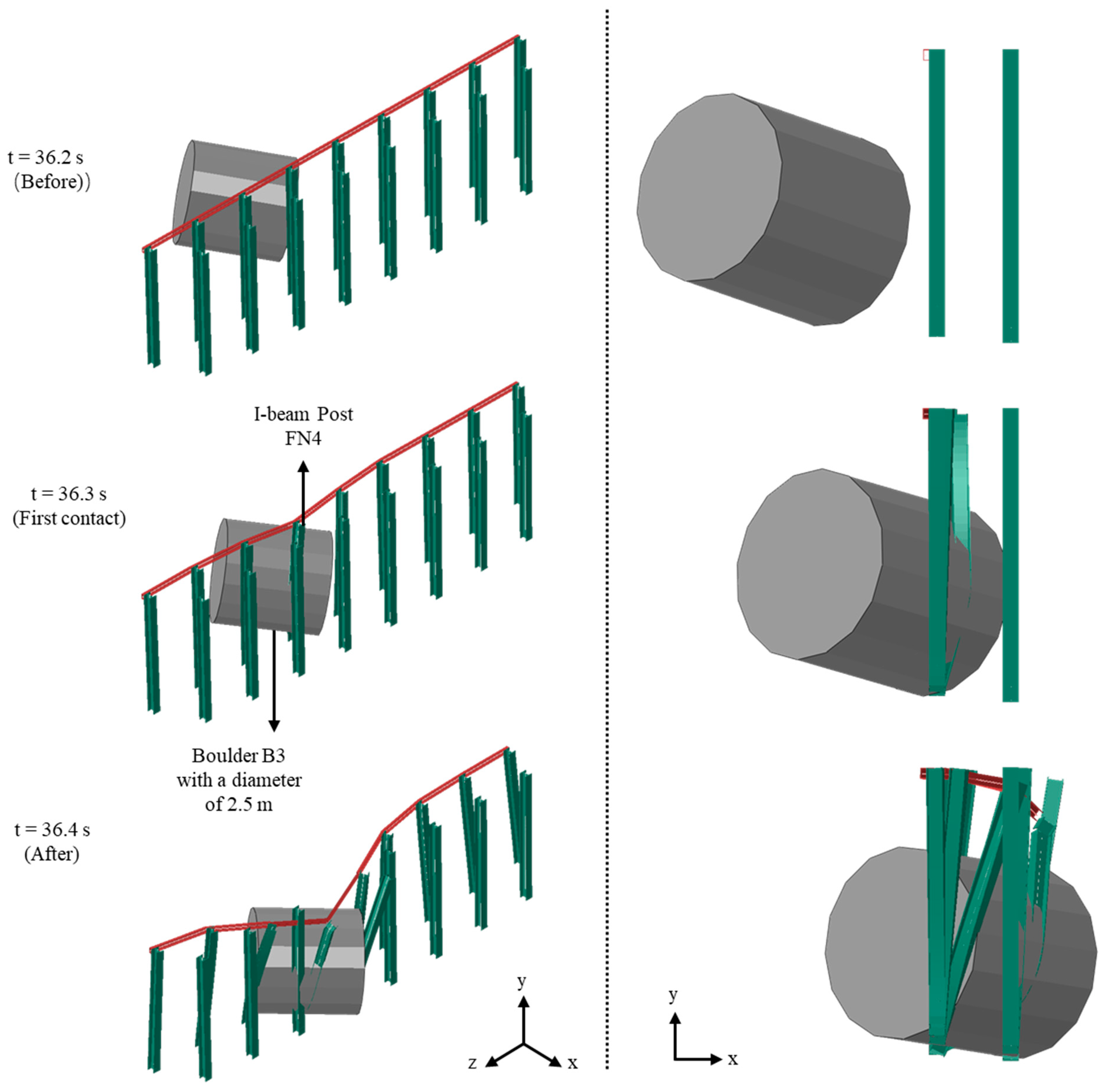
• By accounting for the dynamic nature of debris flows and various impact scenarios, the simulations of boulder–barrier interactions are conducted to assess the performance of I-beam post barriers in Hobart Rivulet. The study identifies weak points in the protective structure using the failure ratio, which measures the proportion of elements failing upon impact. The results show minimal variation in impact forces across different posts, but significant differences in failure ratios, pinpointing FN9 and BN3 as the weakest, with FN9 being critical due to its front-row position.
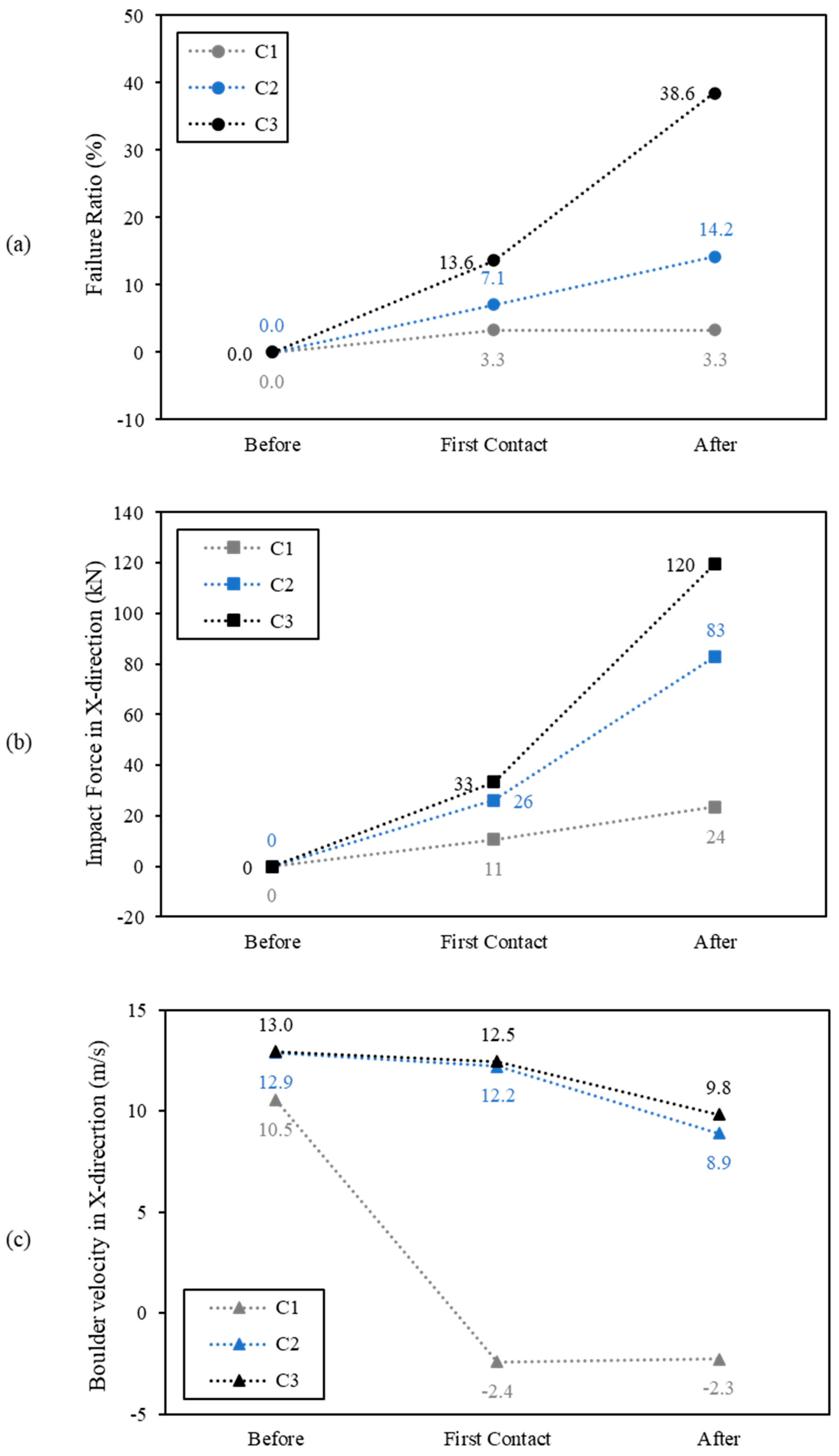
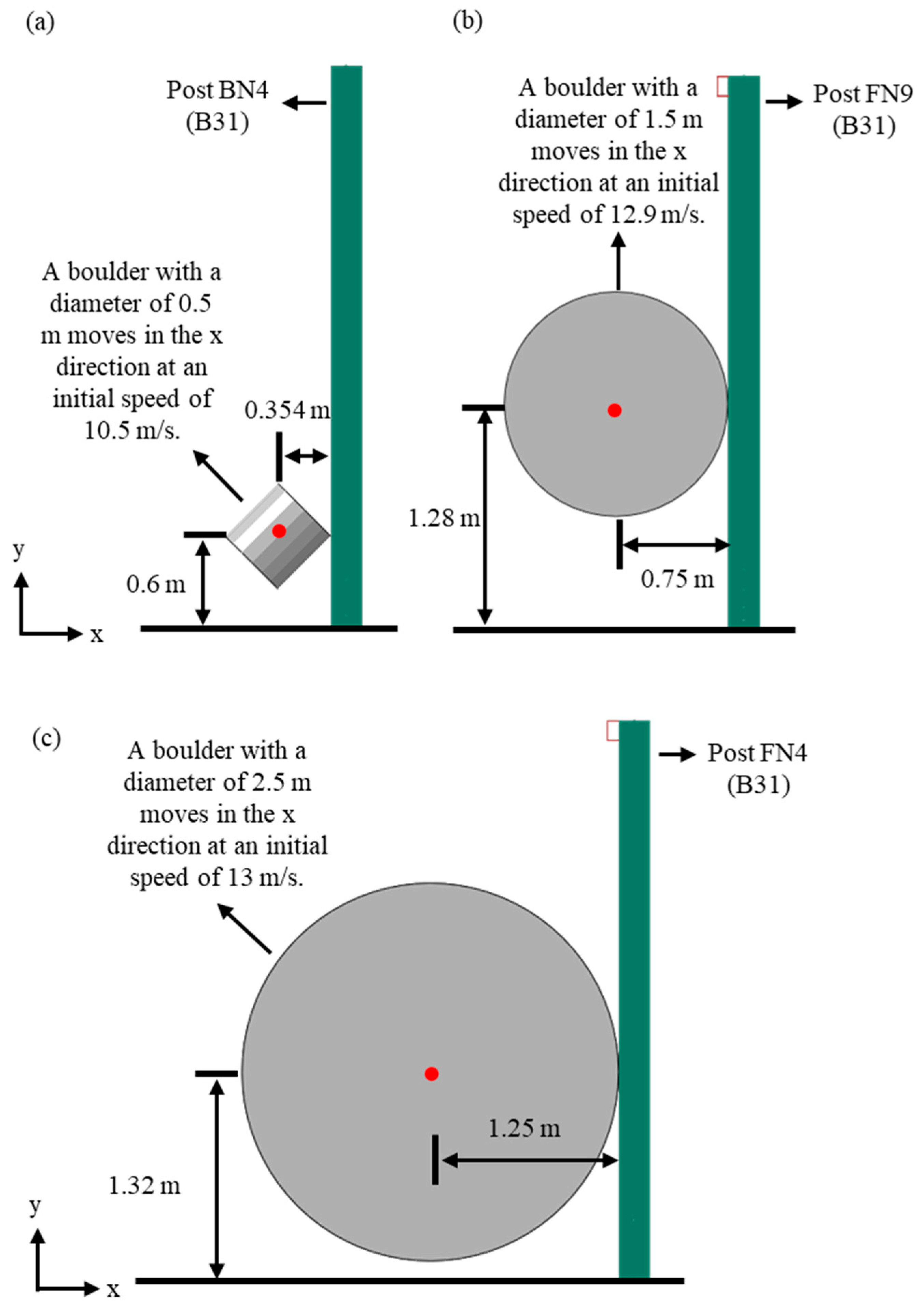
• The simulation results of boulder–barrier interactions also reveal that higher boulder velocities strongly correlate with increased failure ratios and impact forces, while varying impact heights reveal that the middle sections of the posts are more vulnerable. Additionally, larger boulders result in higher failure ratios, while different impact orientations lead to varying structural damages, with orientation (b) yielding the highest failure ratio and orientation (c) the highest impact force.
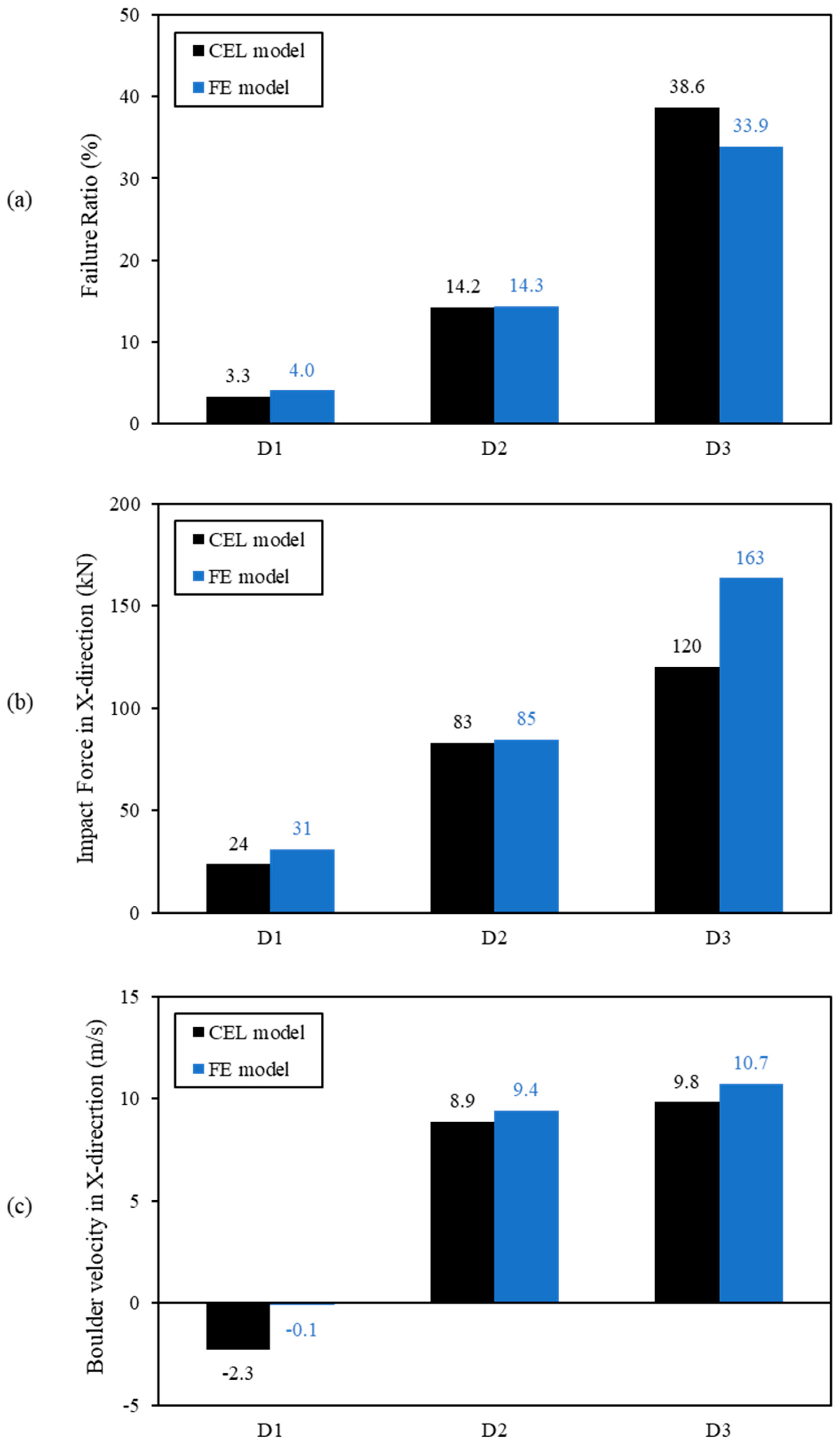
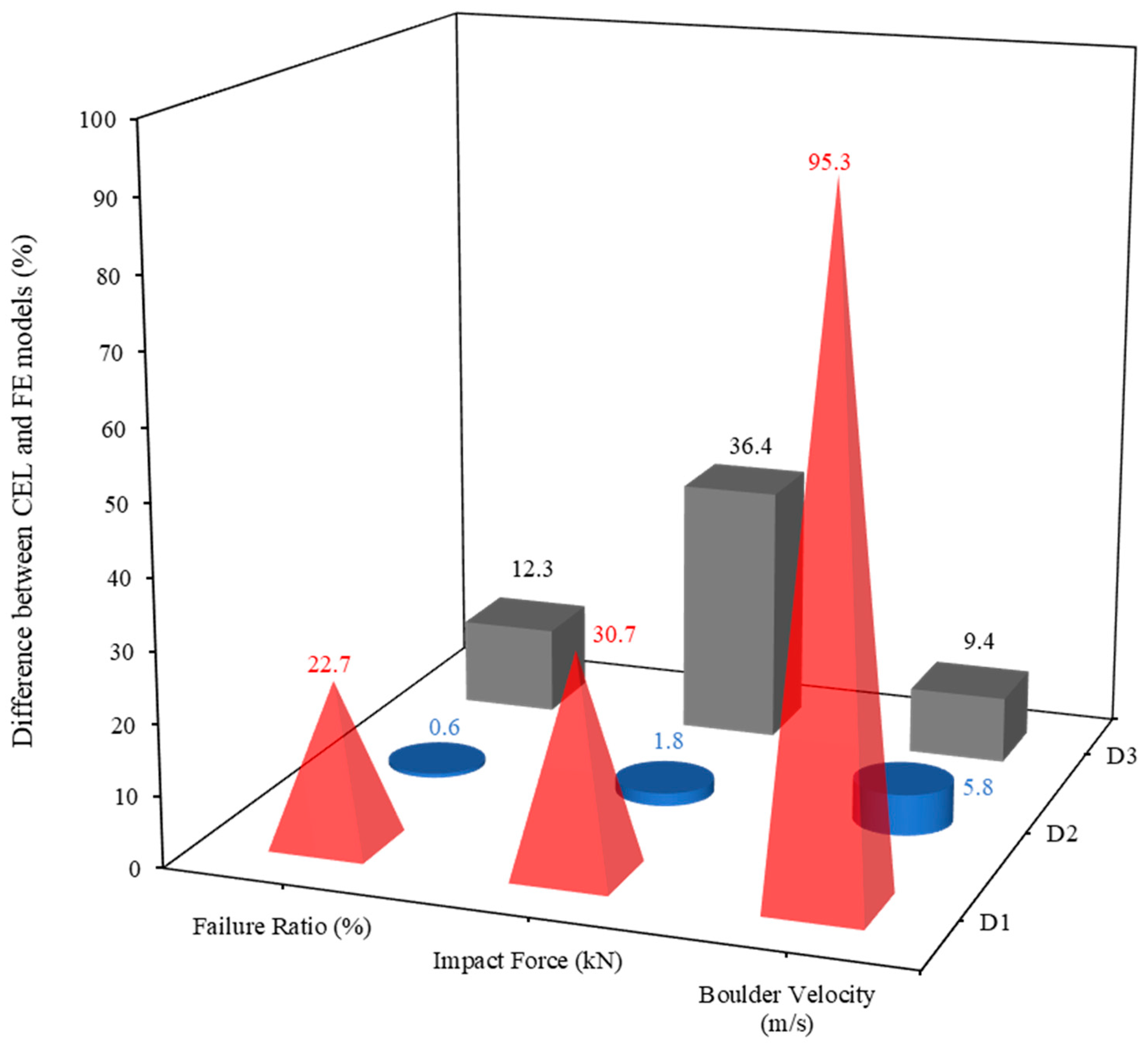
• Numerical models conducted for different boulder sizes (0.5 m, 1.5 m, and 2.5 m) highlight the effectiveness of the CEL model in capturing the complex interactions between debris flow, boulders, and the I-beam barrier on a real rivulet terrain. The findings indicate that larger boulders significantly increase the failure ratio and impact force on the barrier, with failure ratios stabilising at approximately 4%, 65%, and 80% for boulder sizes of 0.5 m, 1.5 m, and 2.5 m, respectively. Notably, the CEL model stands out for handling multiple boulders without assuming impact locations or orientations. Moreover, there is a noticeable difference in the velocities of smaller boulders, indicating the sensitivity of FE models to size variations. The comparative analysis using FE models shows good agreement with CEL results, although the FE models predict slightly higher impact forces and different failure distributions. This complementarity provides valuable insights into the utility of both approaches in enhancing structural resilience and optimising barrier design against debris flow impacts.

Overall, this study provides insights into evaluating the performance of protective barriers against debris flows through CEL and FE analyses, highlighting the critical role of dynamic flow conditions, boulder sizes, and impact orientations in barrier design. Future research should focus on expanding the model’s applicability to various terrain types and debris flow conditions, incorporating different boulder shapes and real-time monitoring data to enhance simulation accuracy. Exploring alternative barrier materials and configurations could further improve structural resilience. Standardising procedures for evaluation and validating models across diverse scenarios remains essential for advancing the field and ensuring the effectiveness of debris flow protective measures in different environments.

References

1. Comiti, F.; Lucía, A.; Rickenmann, D. Large wood recruitment and transport during large floods: A review. Geomorphology 2016, 269, 23–39. [Google Scholar] [CrossRef]
2. Thouret, J.-C.; Antoine, S.; Magill, C.; Ollier, C. Lahars and debris flows: Characteristics and impacts. Earth Sci. Rev. 2020, 201, 103003. [Google Scholar] [CrossRef]
3. Vagnon, F. Design of active debris flow mitigation measures: A comprehensive analysis of existing impact models. Landslides 2020, 17, 313–333. [Google Scholar] [CrossRef]
4. He, J.; Zhang, L.; Fan, R.; Zhou, S.; Luo, H.; Peng, D. Evaluating effectiveness of mitigation measures for large debris flows in Wenchuan, China. Landslides 2022, 19, 913–928. [Google Scholar] [CrossRef]
5. Xu, Y.; Xu, Z.-D.; Guo, Y.-Q.; Jia, H.; Huang, X.; Wen, Y. Mathematical modeling and test verification of viscoelastic materials considering microstructures and ambient temperature influence. Mech. Adv. Mater. Struct. 2022, 29, 7063–7074. [Google Scholar] [CrossRef]
6. Dai, J.; Yang, C.; Gai, P.-P.; Xu, Z.-D.; Yan, X.; Xu, W.-P. Robust damping improvement against the vortex-induced vibration in flexible bridges using multiple tuned mass damper inerters. Eng. Struct. 2024, 313, 118221. [Google Scholar] [CrossRef]
7. Shen, W.G.; Zhao, T.; Zhao, J.D.; Dai, F.; Zhou, G.G. Quantifying the impact of dry debris flow against a rigid barrier by DEM analyses. Eng. Geol. 2018, 241, 86–96. [Google Scholar] [CrossRef]
8. Choi, S.K.; Park, J.Y.; Lee, D.H.; Lee, S.R.; Kim, Y.T.; Kwon, T.H. Assessment of barrier location effect on debris flow based on smoothed particle hydrodynamics (SPH) simulation on 3D terrains. Landslides 2021, 18, 217–234. [Google Scholar] [CrossRef]
9. Zhang, Y.S.; Chen, J.P.; Tan, C.; Bao, Y.D.; Han, X.D.; Yan, J.H.; Mehmood, Q. A novel approach to simulating debris flow runout via a three-dimensional CFD code: A case study of Xiaojia Gully. Bull. Eng. Geol. Environ. 2021, 80, 5293–5313. [Google Scholar] [CrossRef]
10. Vicari, H.; Tran, Q.A.; Nordal, S.; Thakur, V. MPM modelling of debris flow entrainment and interaction with an upstream flexible barrier. Landslides 2022, 19, 2101–2115. [Google Scholar] [CrossRef]
11. Sha, S.; Dyson, A.P.; Kefayati, G.; Tolooiyan, A. Simulation of debris flow-barrier interaction using the smoothed particle hydrodynamics and coupled Eulerian Lagrangian methods. Finite Elem. Anal. Des. 2023, 214, 103864. [Google Scholar] [CrossRef]
12. Liu, C.; Yu, Z.; Zhao, S. A coupled SPH-DEM-FEM model for fluid-particle-structure interaction and a case study of Wenjia gully debris flow impact estimation. Landslides 2021, 18, 2403–2425. [Google Scholar] [CrossRef]
13. Guo, J.; Cui, Y.F.; Xu, W.J.; Yin, Y.Z.; Li, Y.; Jin, W. Numerical investigation of the landslide-debris flow transformation process considering topographic and entrainment effects: A case study. Landslides 2022, 19, 773–788. [Google Scholar] [CrossRef]
14. Luo, G.; Zhao, Y.; Shen, W.; Wu, M. Dynamics of bouldery debris flow impacting onto rigid barrier by a coupled SPH-DEM-FEM method. Comput. Geotech. 2022, 150, 104936. [Google Scholar] [CrossRef]
15. Liang, Z.; Choi, C.E.; Zhao, Y.; Jiang, Y.; Choo, J. Revealing the role of forests in the mobility of geophysical flows. Comput. Geotech. 2023, 155, 105194. [Google Scholar] [CrossRef]
16. Yu, D.; Tang, L.; Chen, C. Three-dimensional numerical simulation of mud flow from a tailing dam failure across complex terrain. Nat. Hazards Earth Syst. Sci. 2020, 20, 727–741. [Google Scholar] [CrossRef]
17. Zhou, J.W.; Cui, P.; Yang, X.G. Dynamic process analysis for the initiation and movement of the Donghekou landslide-debris flow triggered by the Wenchuan earthquake. J. Asian Earth Sci. 2013, 76, 70–84. [Google Scholar] [CrossRef]
18. Li, X.P.; Yan, Q.W.; Zhao, S.X.; Luo, Y.; Wu, Y.; Wang, D.P. Investigation of influence of baffles on landslide debris mobility by 3D material point method. Landslides 2020, 17, 1129–1143. [Google Scholar] [CrossRef]
19. Ng, C.W.W.; Wang, C.; Choi, C.E.; De Silva, W.; Poudyal, S. Effects of barrier deformability on load reduction and energy dissipation of granular flow impact. Comput. Geotech. 2020, 121, 103445. [Google Scholar] [CrossRef]
20. Si, G.W.; Chen, X.Q.; Chen, J.G.; Tang, J.B.; Zhao, W.Y.; Jin, K. The Impact Force of Large Boulders with Irregular Shape in Flash Flood and Debris Flow. KSCE J. Civ. Eng. 2022, 26, 4276–4289. [Google Scholar] [CrossRef]
21. Sha, S.; Dyson, A.P.; Kefayati, G.; Tolooiyan, A. An Equivalent Stiffness Flexible Barrier for Protection Against Boulders Transported by Debris Flow. Int. J. Civ. Eng. 2024, 22, 705–722. [Google Scholar] [CrossRef]
22. Sha, S.; Dyson, A.P.; Kefayati, G.; Tolooiyan, A. Analysis of Debris Flow Protective Barriers Using the Coupled Eulerian Lagrangian Method. Geosciences 2024, 14, 198. [Google Scholar] [CrossRef]
23. Chen, H.X.; Li, J.; Feng, S.J.; Gao, H.Y.; Zhang, D.M. Simulation of interactions between debris flow and check dams on three-dimensional terrain. Eng. Geol. 2019, 251, 48–62. [Google Scholar] [CrossRef]
24. Kefayati, G.; Tolooiyan, A.; Dyson, A.P. Finite difference lattice Boltzmann method for modeling dam break debris flows. Phys. Fluids 2023, 35, 013102. [Google Scholar] [CrossRef]
25. Zhao, L.; He, J.W.; Yu, Z.X.; Liu, Y.P.; Zhou, Z.H.; Chan, S.L. Coupled numerical simulation of a flexible barrier impacted by debris flow with boulders in front. Landslides 2020, 17, 2723–2736. [Google Scholar] [CrossRef]
26. Chehade, R.; Chevalier, B.; Dedecker, F.; Breul, P.; Thouret, J.-C. Effect of Boulder Size on Debris Flow Impact Pressure Using a CFD-DEM Numerical Model. Geosciences 2022, 12, 188. [Google Scholar] [CrossRef]
27. Sha, S.; Dyson, A.P.; Kefayati, G.; Tolooiyan, A. Modelling of debris flow-boulder-barrier interactions using the Coupled Eulerian Lagrangian method. Appl. Math. Model. 2024, 127, 143–171. [Google Scholar] [CrossRef]
28. Greco, M.; Di Cristo, C.; Iervolino, M.; Vacca, A. Numerical simulation of mud-flows impacting structures. J. Mt. Sci. 2019, 16, 364–382. [Google Scholar] [CrossRef]
29. Kokuryo, H.; Horiguchi, T.; Ishikawa, N. Safety assessment method of steel protective structure against large-scale debris flow. Int. J. Prot. Struct. 2022, 13, 509–538. [Google Scholar] [CrossRef]
30. Sun, X.; Chen, M.; Bi, Y.; Zheng, L.; Che, C.; Xu, A.; Tian, Z.; Jiang, Z. Protective effects of baffles with different positions, row spacings, heights on debris flow impact. J. Mt. Sci. 2024, 21, 2352–2367. [Google Scholar] [CrossRef]
31. Lin, C.H.; Hung, C.; Hsu, T.Y. Investigations of granular material behaviors using coupled Eulerian-Lagrangian technique: From granular collapse to fluid-structure interaction. Comput. Geotech. 2020, 121, 103485. [Google Scholar] [CrossRef]
32. Mazengarb, C.; Rigby, T.; Stevenson, M. Geological Survey Technical Report 37: Kunanyi/Mount Wellington Debris Flow Susceptibility and Hazard Assessment; Mineral Resources Tasmania: Rosny Park, Australia, 2023. Available online: https://www.mrt.tas.gov.au/mrtdoc/dominfo/download/TR37/ (accessed on 9 August 2024).
33. Stevenson, M.; Mazengarb, C.; Woolley, R. Historical Assessment of the 1872 Glenorchy Debris Flow: A Basis for Modelling the Large Debris Flow Hazard from the Wellington Range, Hobart; Mineral Resources Tasmania: Rosny Park, Australia, 2016. Available online: https://www.researchgate.net/publication/297549846 (accessed on 9 August 2024).
34. Kain, C.L.; Rigby, E.H.; Mazengarb, C. A combined morphometric, sedimentary, GIS and modelling analysis of flooding and debris flow hazard on a composite alluvial fan, Caveside, Tasmania. Sediment. Geol. 2018, 364, 286–301. [Google Scholar] [CrossRef]
35. Qiu, G.; Henke, S.; Grabe, J. Application of a Coupled Eulerian–Lagrangian approach on geomechanical problems involving large deformations. Comput. Geotech. 2011, 38, 30–39. [Google Scholar] [CrossRef]
36. Chen, X.Y.; Zhang, L.L.; Chen, L.H.; Li, X.; Liu, D.S. Slope stability analysis based on the Coupled Eulerian-Lagrangian finite element method. Bull. Eng. Geol. Environ. 2019, 78, 4451–4463. [Google Scholar] [CrossRef]
37. Tatnell, L.; Dyson, A.P.; Tolooiyan, A. Coupled Eulerian-Lagrangian simulation of a modified direct shear apparatus for the measurement of residual shear strengths. J. Rock Mech. Geotech. Eng. 2021, 13, 1113–1123. [Google Scholar] [CrossRef]
38. Wang, P.Y.; Lian, C.C.; Yue, C.X.; Wu, X.Y.; Zhang, J.M.; Zhang, K.; Yue, Z.F. Experimental and numerical study of tire debris impact on fuel tank cover based on coupled Eulerian-Lagrangian method. Int. J. Impact Eng. 2021, 157, 103968. [Google Scholar] [CrossRef]
39. Huang, Y.; Zhu, C. Simulation of flow slides in municipal solid waste dumps using a modified MPS method. Nat. Hazards 2014, 74, 491–508. [Google Scholar] [CrossRef]
40. Zhu, C.; Huang, Y.; Zhan, L.-t. SPH-based simulation of flow process of a landslide at Hongao landfill in China. Nat. Hazards 2018, 93, 1113–1126. [Google Scholar] [CrossRef]
41. Kang, D.H.; Hong, M.; Jeong, S. A simplified depth-averaged debris flow model with Herschel-Bulkley rheology for tracking density evolution: A finite volume formulation. Bull. Eng. Geol. Environ. 2021, 80, 5331–5346. [Google Scholar] [CrossRef]
42. Chen, Y.; Zhang, L.; Wei, X.; Jiang, M.; Liao, C.; Kou, H. Simulation of runout behavior of submarine debris flows over regional natural terrain considering material softening. Mar. Georesources Geotechnol. 2023, 41, 175–194. [Google Scholar] [CrossRef]
43. Hussin, H.; Quan Luna, B.; Van Westen, C.; Christen, M.; Malet, J.-P.; Van Asch, T.W. Parameterization of a numerical 2-D debris flow model with entrainment: A case study of the Faucon catchment, Southern French Alps. Nat. Hazards Earth Syst. Sci. 2012, 12, 3075–3090. [Google Scholar] [CrossRef]
44. Tang, J.; Cui, P.; Wang, H.; Li, Y. A numerical model of debris flows with the Voellmy model over a real terrain. Landslides 2023, 20, 719–734. [Google Scholar] [CrossRef]
45. Kafle, J.; Kattel, P.; Mergili, M.; Fischer, J.-T.; Pudasaini, S.P. Dynamic response of submarine obstacles to two-phase landslide and tsunami impact on reservoirs. Acta Mech. 2019, 230, 3143–3169. [Google Scholar] [CrossRef]
46. Zhu, C.; Huang, Y.; Sun, J. A granular energy-controlled boundary condition for discrete element simulations of granular flows on erodible surfaces. Comput. Geotech. 2023, 154, 105115. [Google Scholar] [CrossRef]
47. Wang, F.; Wang, J.D.; Chen, X.Q.; Zhang, S.X.; Qiu, H.J.; Lou, C.Y. Numerical Simulation of Boulder Fluid–Solid Coupling in Debris Flow: A Case Study in Zhouqu County, Gansu Province, China. Water 2022, 14, 3884. [Google Scholar] [CrossRef]
48. Schilirò, L.; De Blasio, F.V.; Esposito, C.; Scarascia Mugnozza, G. Reconstruction of a destructive debris-flow event via numerical modeling: The role of valley geometry on flow dynamics. Earth Surf. Process. Landf. 2015, 40, 1847–1861. [Google Scholar] [CrossRef]
49. Tayyebi, S.M.; Pastor, M.; Stickle, M.M.; Yagüe, Á.; Manzanal, D.; Molinos, M.; Navas, P. Two-phase SPH modelling of a real debris avalanche and analysis of its impact on bottom drainage screens. Landslides 2022, 19, 421–435. [Google Scholar] [CrossRef]
50. Dai, Z.L.; Huang, Y.; Cheng, H.L.; Xu, Q. 3D numerical modeling using smoothed particle hydrodynamics of flow-like landslide propagation triggered by the 2008 Wenchuan earthquake. Eng. Geol. 2014, 180, 21–33. [Google Scholar] [CrossRef]
51. Pellegrino, A.M.; di Santolo, A.S.; Schippa, L. An integrated procedure to evaluate rheological parameters to model debris flows. Eng. Geol. 2015, 196, 88–98. [Google Scholar] [CrossRef]
52. Ng, C.W.; Liu, H.; Choi, C.E.; Kwan, J.S.; Pun, W.K. Impact dynamics of boulder-enriched debris flow on a rigid barrier. J. Geotech. Geoenviron. Eng. 2021, 147, 04021004. [Google Scholar] [CrossRef]
53. Iverson, R.M. The physics of debris flows. Rev. Geophys. 1997, 35, 245–296. [Google Scholar] [CrossRef]
54. Takahashi, T. Debris Flow: Mechanics, Prediction and Countermeasures; Taylor & Francis: Abingdon, UK, 2007. [Google Scholar] [CrossRef]
55. AS/NZS 3679.1:2016; Structural Steel. Part 1: Hot-Rolled Bars and Sections. Australian Steel Institute: Pymble, Australia, 31 December 2015. Available online: https://www.steel.org.au/resources/elibrary/library/as-nzs-3679-1-2016-structural-steel-part-1-hot-rolled-bars-and-sections/ (accessed on 9 August 2024).
56. ABAQUS. Abaqus Analysis User’s Guide, Version 6.14; Dassault Systèmes Simulia Corp.: Providence, RI, USA, 2014; Available online: http://62.108.178.35:2080/v6.14/books/usb/default.htm (accessed on 9 August 2024).
Figure 1. The overview of the proposed procedure for the performance assessment.
Sustainability 16 07332 g001
Figure 2. (a) Model configuration for simulating the boulder-enriched debris flow tests [22,27]; (b) Comparison of experimental and CEL simulation results in the time history of impact force for Test D; (c) Comparison of experimental and CEL simulation results in the velocities of debris front and first arrival boulder.
Sustainability 16 07332 g002
Figure 3. Topographic map highlighting the study area (red area) along the Hobart Rivulet (blue lines) (Left); Isometric view of the study area (Right).
Sustainability 16 07332 g003
Figure 4. The CEL model of Hobart rivulet for flow velocity estimation. (a) Eulerian domain and initial debris flow; (b) the model configuration and flow velocity test locations (red points).
Sustainability 16 07332 g004
Figure 5. The time history of debris flow velocity at the specific test locations along the flow path.
Sustainability 16 07332 g005
Figure 6. (a) The selected existing protective barrier along the Hobart Rivulet (Left: front view); Two rows of vertical posts, with a cross flange installed on the top of the front row only (Right: side view); (b) The model of the selected I-beam post barrier for the performance analysis.
Sustainability 16 07332 g006
Figure 7. The model of boulder–structure interaction for evaluating the weakest post within the barrier (used Test FN1 as an example): the geometry of the model (top) and side view of the model for one I-beam post (bottom).
Sustainability 16 07332 g007
Figure 8. Comparison of the failure ratio and the maximum impact force between I-beam posts.
Sustainability 16 07332 g008
Figure 9. The model of boulder–structure interaction for investigating the effect of boulder velocity: the geometry of the model (top) and side view of the model for FN9 I-beam post (bottom).
Sustainability 16 07332 g009
Figure 10. Comparison of the failure ratio and the maximum impact force at different boulder velocities.
Sustainability 16 07332 g010
Figure 11. The model of boulder–structure interaction for investigating the effect of boulder impact height (using the case of the height of 0.5 m as an example).
Sustainability 16 07332 g011
Figure 12. Comparison of the failure ratio and the maximum impact force at various boulder impact heights.
Sustainability 16 07332 g012
Figure 13. The model of boulder–structure interaction for investigating the effect of boulder size (using the case S3 as an example).
Sustainability 16 07332 g013
Figure 14. Comparison of the failure ratio and the maximum impact force between I-beam posts at different boulder sizes.
Sustainability 16 07332 g014
Figure 15. The model of boulder–structure interaction for investigating the effect of boulder impact orientation: (a) 45-degree inclination; (b) circular surface at 90 degrees to the Y-axis; (c) circular surface at 90 degrees to the X-axis; (d) circular surface at 90 degrees to the Z-axis.
Sustainability 16 07332 g015
Figure 16. Comparison of the failure ratio and the maximum impact force between I-beam posts at different boulder impact orientations.
Sustainability 16 07332 g016
Figure 17. The CEL model of flow–boulder–barrier interaction on the Hobart rivulet terrain (Using Case C2 as an example).
Sustainability 16 07332 g017
Figure 18. Comparison of the failure ratio between cases at different boulder sizes at 50 s.
Sustainability 16 07332 g018
Figure 19. Visualisation of failed elements of the barrier after boulder impacts at 50 s (Left) and comparison of the barrier performance at 0 s and 50 s (Right): dark blue–non-failed elements, grey–failed elements, at t = 50 s; light blue–non failed elements, at t = 0 s.
Sustainability 16 07332 g019
Figure 20. Visualisation of the collision between the first boulder and I-beam post barrier for Case C1, capturing the moments before, during, and after the initial impact for 0.2 s: isometric view (Left); side view (Right).
Sustainability 16 07332 g020
Figure 21. Visualisation of the collision between the first boulder and I-beam post barrier for Case C2, capturing the moments before, during, and after the initial impact for 0.2 s: isometric view (Left); side view (Right).
Sustainability 16 07332 g021
Figure 22. Visualisation of the collision between the first boulder and I-beam post barrier for Case C3, capturing the moments before, during, and after the initial impact for 0.2 s: isometric view (Left); side view (Right).
Sustainability 16 07332 g022
Figure 23. Comparative analysis for three cases (C1, C2, and C3) before, during, and after the boulder’s collision with the barrier: (a) failure ratio; (b) impact force; and (c) boulder velocity.
Sustainability 16 07332 g023
Figure 24. The configurations of the FE boulder–barrier interaction models, based on CEL model observations: (a) a boulder with a diameter of 0.5 m placed at the height of 0.6 m with 45-degree inclination moves in the x direction at an initial speed of 10.5 m/s; (b) a boulder with a diameter of 1.5 m placed at the height of 0.75 m with circular surface at 90 degrees to the Z-axis moves in the x direction at an initial speed of 12.9 m/s; (c) a boulder with a diameter of 2.5 m placed at the height of 1.32 m with a circular surface at 90 degrees to the Z-axis moves in the x direction at an initial speed of 13 m/s.
Sustainability 16 07332 g024
Figure 25. Comparative analysis for three scenarios: before (D1), during (D2), and after (D3) the boulder’s collision with the barrier: (a) failure ratio; (b) impact force; and (c) boulder velocity.
Sustainability 16 07332 g025
Figure 26. Comparison of percent difference between the CEL and FE models for failure ratio, impact force, and boulder velocity across three scenarios (D1, D2, D3).
Sustainability 16 07332 g026
Figure 27. Visualisation and comparison of failed elements of the barrier at 0.2 s after the first boulder impacts between two approaches with non-failed elements in blue and failed elements in grey: (a) CEL model; (b) FE model.
Sustainability 16 07332 g027