Abstract
An aerated greenhouse ecosystem, often referred to as a Living Machine®, is a technology for biological wastewater treatment within a greenhouse structure that uses plants with their roots submerged in the wastewater. This system has a small footprint relative to traditional onsite wastewater treatment systems and constructed wetland, can treat high-strength wastewater, and can provide a high level of treatment to allow for reuse for purposes such as irrigation, toilet flushing, and landscape irrigation. Synthetic and actual craft beverage wastewaters (wastewater from wineries, breweries, and cideries) were examined for their treatability in bench-scale greenhouse ecosystems. The tested wastewater was high strength with chemical oxygen demands (COD) concentrations of 1120 to 15,000 mg/L, total nitrogen (TN) concentrations of 3 to 45 mg/L, and total phosphorus (TP) concentrations of 2.3 to 90 mg/L. The COD, TN, and TP concentrations after treatment ranged from below 125 to 560 mg/L, 1.5 to 15 mg/L, and below 0.25 to 7.8 mg/L, respectively. The results confirm the ability of the aerated greenhouse ecosystem to be a viable treatment system for craft beverage wastewater and it is estimated to require 54 and 26% lower hydraulic retention time than an aerobic lagoon and a low temperature, constructed wetland, respectively, the types of systems that would likely be used for this type of wastewater for onsite locations.
1. Introduction
A greenhouse ecosystem, commonly known as a Living Machine®, uses plants within a greenhouse growing in tanks of wastewater for treatment [1,2]. Because the rhizosphere is the critical treatment component, plants with root systems with higher surface area typically result in better treatment capacity [3,4]. Both anaerobic and aerobic zones exist in a greenhouse ecosystem, which allows for carbon oxidation, nitrification, and denitrification [1]. Plants also contribute to nitrogen uptake. Phosphorus removal is typically achieved by precipitation and plant uptake [5]. The wastewater can be treated to an extent that allows for reuse as irrigation water or toilet flushing. The greenhouse ecosystem has been demonstrated on blackwater [6,7], dairy wastewater [8], and poultry wastewater [9] and is theorized to have a smaller footprint and be more economical than other high-strength, low-flow onsite wastewater treatment processes.
Craft beverage wastewater is high strength, with an average, approximate chemical oxygen demand (COD) of 3000 mg/L [10]. The wastewater is produced from excess raw products, equipment cleaning, product processing, packaging preparation, and off-specification products discharged to the drain. Most of the winery and cidery wastewater is typically produced during half of the year, after the fall harvest. Beer wastewater is typically produced throughout the year [11].
Table 1 summarizes the characteristics of craft beverage wastewater. The data were obtained from a Michigan Department of Environmental Quality study that had five sample collection sites [10]. Skornia et al. [12] collected wastewater from one site and noted that the values collected were lower than the average national values but matched the values from the Michigan study. Bakare et. al. [13] had one sample collection site and used the literature to confirm the values. Brito et. al. [14] had three sample collection points and used additional sources for comparison. Hard cider wastewater was difficult to characterize as there were few resources and most studies examined the solids portions produced.

Table 1.
General craft beverage wastewater characteristics [10,12,13,14].
The variability of craft beverage wastewater flow and characteristics from low-volume producers makes it difficult to use a conventional onsite wastewater treatment system such as a septic tank and drain field. Building a traditional activated sludge or fixed film treatment plant onsite at a low-volume producer is expensive, difficult to operate, and requires a relatively large area.
The greenhouse ecosystem is demonstrated to treat high-strength food processing wastewater but the literature on its application for craft beverage wastewater was not found. This research was a proof-of-concept study on its applicability to this industry, to determine possible pollutant removal mechanisms and whether this small system is as effective as a larger system.
2. Materials and Methods
The general tasks of this research include the following steps.
- Design a greenhouse ecosystem for craft beverage wastewater, using the literature values from other high-strength wastewaters.
- Choose the best native, non-invasive plants to use for the greenhouse ecosystem.
- Determine the characteristics of winery, brewery, and cidery wastewaters to develop synthetic wastewaters (SWWs). SWWs were used to determine the effect of specific wastewater constituents on treatment and plants.
- Collect and treat actual winery, brewery, and cidery wastewater to determine if any constituents that were not in the SWW negatively impact the greenhouse ecosystem.
The design and construction of the bench-scale greenhouse ecosystem was developed based on the literature pertaining to the use of similar treatment technologies for food processing wastewater and references on native plant tolerance to the harsh environment. SWW was developed and used to test the capacity of the system and the impact of craft-beverage specific wastewater components. Actual craft beverage wastewaters were then examined to verify treatability. Details are provided in the sequential subsections.
2.1. Loading and System Configuration
The wastewater loading and plant selection determined the volume, dimensions, and flow to the bench-scale greenhouse ecosystem. A loading of 0.61 kg/m3-d was estimated from the typical COD concentration in winery wastewater (Table 1) and the literature loading values for a greenhouse ecosystem, constructed wetlands, and biofilters receiving high-strength wastewater (Table 2). The configuration and general layout were determined by surface area and depth requirements for the selected plants.
Table 2.
Literature loading values for high-strength wastewater.
This project had three parallel, independent treatment trains, each consisting of three reactors. Figure 1 is a plan view schematic of the system. The reactors were 208 L (55-gallon) drums with 189.3 L (50 gallons) of operating volume obtained from Grainger (Lake Forest, IL, USA). These reactors were found to have a depth adequate for unrestricted root growth for the selected plants. From the selected loading, 0.61 kg/m3-d, the flow rate to each reactor was 20.4 L/d (5.4 gal/day), which flowed only during the day (08:00 AM to 08:00 PM). The resulting hydraulic detention time was approximately 9 days.
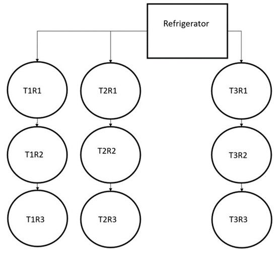
Figure 1.
System schematic with reactor name labels. Arrows show direction of water movement. Notes: T: Train; R: Reactor.
An aeration system was added to the reactors in each train after about a month of operation to reduce odors. The aeration system was operated during the day (12 h), in sync with the lights and feed pumps. A 6592 L/min (1744 GPM) aeration pump (Simple Deluxe (Duarte, CA, USA) pump, model number LGPUMPAIR110) was used to provide the air through a manifold to each reactor. Within each reactor, a 2-in aeration stone (Pawfly [Raleigh, NC, USA] Aquarium Air Stones Balls, 2 in diameter), was connected to the tubes and placed at the bottom of the reactor. Each aeration stone provided roughly 733 L/min (194 GPM) of air. The dissolved oxygen (DO) was measured daily to monitor the reactor environment to reduce the risk of noxious gasses forming again as discussed in Section 2.4.
The influent wastewater was stored in 22.7 L (6-gallon) buckets in a refrigerator at a temperature of approximately 4 °C, typically for up to 3 days, to minimize microbial growth. The wastewater was pumped directly from the refrigerator into the first reactor of each train. The pumps were Cole-Parmer Masterflex® (Vernon Hills, IL, USA) No. 7553-80, 1–100 RPM, with Masterflex® Model 7017-20 pump heads and Masterflex® tubing, size L/S 17. The same model pump was used to transfer the water from the first reactor into the second reactor and second to the third. There was a gravity outlet on the side of the third reactor that allowed the effluent water to flow into a storage container.
A Roleadro (Amazon.com) full-spectrum grow light (HYD-MINI100*10W-W) was hung approximately 7.5 feet above the top of each reactor (9 total lights) to simulate natural sunlight. The lights were on a 12 h cycle, starting at 8 AM and ending at 8 PM. The resulting light intensity at the water surface measured using Photone 0.5.2 [19] averaged 100 PPFD, which is in then general acceptable range, especially as plants become taller [20].
2.2. Plant Choice and Health Monitoring
The plants were chosen by performing a literature review using the following criteria: cold tolerance (to allow for treatment over winter months when the temperature in the greenhouse lowers), pruning tolerance, and non-invasive/native in the northern region of the US.
The selected plants were Schoenoplectus pungens [4,20] (three square bulrush, also known as Scirpis pungens), Acorus americanus (American sweetflag), Decodon verticillatus (swamp loosestrife), Typha augustifolia (cattail) [4,21,22], Penstemon digitalis (foxglove beard tongue), and Spirodela polyrhiza (duckweed species), a volunteer species that grew on its own in the system and was not initially planted [4,23]. The plants were purchased from Stantec Native Plants in Walkerton, Indiana, USA.
The plants were inserted into plastic poultry fence. The fence had extra holes cut into it to allow for the plant roots to be inserted without damage to the plant. During experimentation, the plants were monitored visually to determine health. The three growth indicators were leaf color, leaf texture, and plant elongation. Plant leaves change colors, typically to yellow or brown, if stressed. If water is lacking, the leaves become dry and wrinkled. If absorbing too much water, the leaves become soft. Plant elongation occurs when lacking light. This leads to yellowing leaves near the base of the plant that will be more likely to fall off. Photographs of the plants in each reactor were taken every day to allow for comparisons of health over time.
2.3. Research Phases
All trains operated identically for the first approximately 45 days with SWW to allow the systems to equilibrate. Train 1 served as a control as it continued to operate under these same conditions for the entire research period. The feed to trains 2 and 3 were periodically changed to determine the effect of specific wastewater constituents and the effects of actual wastewaters.
The research phases and their dates are listed below.
- Phase 1: 3/20/23–4/6/23
- o
- All trains managed identically, receiving SWW
- Phase 2: 4/13/23–5/17/23
- o
- Train 1: SWW
- o
- Train 2: SWW with COD spike to mimic winery wastewater
- o
- Train 3: SWW with nutrient spike to mimic brewery wastewater
- Phase 3: 5/31/23–6/22/23
- o
- Train 1: SWW
- o
- Train 2: SWW spiked with COD and nutrients, representing winery wastewater
- o
- Train 3: SWW spiked with nutrients and salt spike, representing cidery wastewater
- Phase 4: 7/14/23–8/21/23
- o
- Train 1: SWW
- o
- Train 2: actual winery wastewater
- o
- Train 3: actual cidery wastewater
- Phase 5: 10/20/23–11/15/23
- o
- Train 1: SWW
- o
- Train 2: actual brewery wastewater
- o
- Train 3: SWW, recovery after actual cidery wastewater
The literature review (Table 1) determined the components of the SWW and its variations to represent winery, cidery, and brewery wastewaters (Table 3). This assumed the COD of the SWW was 3200 mg/L and the amount of alcohol in the wine 16% (volume basis). An assumption of 16% ABV wine was based on the higher average of wine produced from riesling grapes, which is the most popular wine produced in Michigan, where this experiment was performed. This resulted in an estimated wine content in the wastewater of 1.3% (volume basis). This is a reasonable estimate due to the high range of wastewater produced per liter of wine. For one liter of wine, 0.2–14 L of wastewater can be produced [24].
Table 3.
Synthetic wastewater recipes to produce 1 L of SWW.
The diluted juice was a white grape concentrate preserved with sulfur dioxide (Global Vitners, Inc., St Catharines, ON, Canada), which was diluted at a ratio of 1:20, juice concentrate to water. However, this amount of diluted juice did not provide enough nitrogen or phosphorus, based on Table 1, hence the need for their addition. The nitrogen fertilizer, Menards Premium, contained 22.0% total nitrogen in the form of urea nitrogen, 10.0% soluble potash (K2O), and 1.0% iron. Acros Organics dibasic and anhydrous sodium phosphate was used, which was 99+% sodium phosphate.
2.4. Analytical Methods
Daily sampling for pH, temperature, and dissolved oxygen was performed in each reactor. The pH was measured using a HACH (Romeoville, IL, USA) sensION+™ portable pH meter with a Sension+5051T pH electrode [25]. The DO and temperature were measured using a HACH HQ1130 DO/1 Channel with an LDO 10101 probe [26]. The probe’s minimum limit was 0.1 mg/L. Probe measurements were taken at the same place in every reactor and wastewater bucket, in the center of each drum, roughly 2–3 inches below the surface of the water.
Water samples were taken, on average, 3–5 times per research phase to measure COD, total nitrogen (TN), ammonia, nitrite, nitrate, and total phosphorus (TP) using HACH TNT kits TNT 823, TNT 831, TNT 826, TNT 839, TNT 835, and TNT 844, respectively. COD, ammonia, and nitrate are US EPA approved methods. A HACH DR6000 UV VIS Spectrophotometer was used to obtain the concentrations.
Water samples were collected by taking a clean plastic sample collection bottle and dipping it a few cm beneath the surface in the center of the reactor. Samples were either analyzed immediately or stored at 4 °C for up to 24 h before analyzing so that a chemical preservative was not necessary. Three replicates were chosen using a random number generator during each sampling event, representing a 25% replication rate. Standards and blanks (DI water) were also performed at a 5% replication rate. If the replicates were not within 10% of each and/or the standards and blanks were not within 10% of the expected value, the analyses were rerun.
2.5. Statistical Analysis
Statistical analyses were conducted by the Michigan State College of Agriculture and Natural Resources Statistics Consulting Center. The average value for each parameter in each phase was calculated. If a value was below the method detection limit (BDL), it was calculated as midway between zero and the detection limit. Data were analyzed with the R statistical software 2023.09.1+494 using a linear mixed effect model. An ANOVAs revealed significant main effects at alpha level of 0.05.
3. Results and Discussion
The wastewater analysis is presented in six sections: COD, TN, ammonia, nitrite, nitrate, and TP. Within each section, the average influent and effluent values, number of data points, standard deviation, percent removal, and percent removal standard deviation are shown. Regarding the control train, Train 1, the values for each wastewater characteristic in each research phase are combined as the feed was consistent throughout the entire research period. Data in the tables are marked as statistically different by using superscripts of a and b between the influent and effluent. Data with no superscripts indicate that there is not a statistical difference between the values. A statistical analysis of organic nitrogen was not performed as this was calculated from other values found.
3.1. COD Analysis
COD data, shown in Table 4, was used to represent the general organic carbon content of the wastewater. Biochemical oxygen demand measures biodegradable organic carbon and is used in most regulatory applications but COD was used exclusively for this research.
Table 4.
COD analysis statistics.
The average COD of SWW in each phase that did not receive a COD spike ranged from 1100 to 1400 mg/L, across all phases. There were no statistical differences between the influent and effluent for the SWW in all trains, likely because of the high standard deviations ranging from 600 to 1000 and initial start-up issues. The variation may have also occurred from COD degradation over the three-day storage period, even though stored at a low temperature. However, there was still a decreasing trend between the influent and effluent concentrations, 88, 67, and 74% for Trains 1, 2, and 3, respectively. Only two reactors were needed to remove the COD from the SWW. In train 1, the first, second, and third reactor removed 76, 45, and 6.2% of each reactor’s influent value, respectively. In train 2, the first, second, and third reactor removed 11, 46, and 33% of each reactor’s influent value, respectively. In train 3, the first, second, and third reactor removed 28, 40, and 39% of each reactor’s influent value, respectively.
The SWW that was spiked with COD and COD and nutrients resulted in influent values of approximately 4500 mg/L and excellent, statistically significant removals. The COD removals for the SWW spiked with COD in Reactors 1, 2, and 3 were approximately 74, 49, and 10%, respectively. The removals for the SWW spiked with COD and nutrients in Reactors 1, 2, and 3 were 82, 59, and 38%, respectively.
The SWW spiked with nutrients and the SWW spiked with nutrients and salt also showed statistically significant removals, which were 89 and 90%, respectively. Both had similar trends between reactors within a train. Removals for Reactors 1, 2, and 3, relative to each reactor’s influent value for the SWW spiked with nutrients, were 76, 44, and 20%, respectively. For the SWW spiked with nutrients and salt, the removals for Reactors 1, 2, and 3, relative to each reactor’s influent value were 52, 70, and 33%, respectively. Altering COD, nutrient, and salt levels to those expected to be in craft beverage wastewater did not negatively impact COD removal, when compared to the control. Results also indicate that there is better removal of COD with higher nutrients.
The actual winery, brewery, and cidery wastewater had tediously higher COD values than expected, 7949, 12,981, and 15,222, respectively. The cidery influent also had substantial variation, which was likely due to the disposal of an off-speciation batch during sample collection. However, excellent statistically significant removals in the high 90% range were still achieved for all actual wastewaters. For the winery wastewater, the removal in Reactors 1, 2, and 3, relative to each reactor’s influent value, were 86, 83, and 20%, respectively. For brewery wastewater, the removals in Reactors 1, 2, and 3, relative to each reactor’s influent value, were relatively consistent, at 61, 78, and 69% for Reactors 1, 2, and 3, respectively. Cidery wastewater had an inverse pattern between the reactors as the removal for Reactors 1, 2, and 3, relative to each reactor’s influent value, were 42, 82, and 81%, respectively. The different treatment distributions between reactors with the higher influent COD levels was probably due to oxygen limitations. The very high COD in the cidery wastewater also caused the plants to dry and wither while maintaining the original leaf color, likely from oxygen deprivation, to be discussed in Section 3.4. Once cidery wastewater addition was discontinued, the original SWW was reintroduced into that train and the plants began to recover.
Overall, COD results indicate superior performance under all conditions, although continuous treatment of very-high-strength wastewater could not be sustained due to damage to the plants. However, a high-strength brief slug is treatable, as indicated by the actual cidery experiment. Results also indicate that a larger loading, resulting in a smaller reactor, could be achieved if COD is the main treatment goal.
3.2. Nitrogen Analysis
One goal of using three reactors in each train was to maintain multiple environments to encourage nitrification and denitrification. Nitrification, ammonia conversion to nitrate, occurs under aerobic conditions when carbon is limiting [27]. Denitrification, nitrate conversion to nitrogen gas (N2), occurs under anoxic conditions and carbon is required [27]. Additionally, plant uptake of ammonia and nitrate can occur. Another pathway of nitrogen removal is anammox, where nitrite and ammonia are converted directly into N2. However, ethanol and other alcohols, as well as a high concentration of nitrite, can inhibit anammox [28].
3.2.1. Total Nitrogen
Wastewater TN levels are specific to the type of craft beverage and can originate from malts and adjuncts, used in breweries, and nitrogen to support yeast growth that may be added to any fermenting process [29]. Wastewater TN is also very processor specific as it is at high concentrations in some cleaning agents [30,31,32]. Table 5 shows the TN data.
Table 5.
Total nitrogen analysis statistics.
There were no statistical differences between the influent and effluent for any of the experiments. However, there was a decreasing TN trend in almost all the treatment trains.
For the SWW only experiments, there was an overall average TN reduction of 64, 59, and 32% through the control system, trains 1, 2, and 3, respectively. Reactors 1, 2, and 3 in train 1 removed an average TN of 7, 40, and 35%, respectively. In train 2, the first, second, and third reactor removed 34, 49, and −22% of each reactor’s influent value, respectively. In train 3, the first, second, and third reactor removed −14, 50, and −18.4% of each reactor’s influent value, respectively.
TN was very consistently removed for the reactor with SWW spiked with nutrients and SWW spiked with salt and nutrients, with values of 76 and 64%, respectively. Removals in Reactors 1, 2, and 3, relative to each reactor’s influent values for the SWW spiked with nutrients and SWW spiked with salt and nutrients experiments, were 21, 43, and 46, and 47, −2, and 33%, respectively. These removals were similar to experiments with just SWW, indicating that increasing the salinity and TN from approximately 6 mg/L to 11 and 15 mg/L, in the SWW spiked with nutrients and the SWW spiked with salt and nutrients, respectively, did not negatively impact TN removal. However, the TN removals for SWW spiked with COD and SWW spiked with COD and nutrients were low, 31 and 11%, respectively. Removals in Reactors 1, 2, and 3, relative to each reactor’s influent value for the SWW spiked with COD and SWW spiked with COD and nutrients, were 30, 12, and −12% and −105, 38, and 30%, respectively. For the SWW spiked with COD, a substantial amount of COD remained in the effluent, indicating that biotic nitrification may have never started. However, for the experiment with SWW spiked with COD and nutrients, the effluent COD was BDL, making it unclear why TN was not removed.
The SWW recovery experiment in Train 3 had an increase in TN by approximately 50%, unlike the other experiments with the same feed, SWW. The changes in Reactors 1 2, and 3, relative to each reactor’s influent value, were −8.2, 0.7, and −42%, respectively. However, this experiment occurred after the one with actual cidery wastewater, which had a tremendously high COD, during which plant damage and sloughing was observed. Consequently, this experiment reinforces this hypothesis that the variability in TN was likely due to plant residuals in the analytical samples.
Approximately 50% of TN was removed from the brewery wastewater. The amount removed in Reactors 2 and 3, relative to the train influent, were 39 and 22%, relative to each reactor’s influent value, respectively (the value for Reactor 1 is not available). For the cidery wastewater, 88% of TN was removed. Reactors 1, 2, and 3 removed 53, 48, and 52% relative to each reactor’s influent value. For unknown reasons, the high COD levels in this wastewater did not appear to have a negative impact on TN removal as in the SWW with the COD spikes, which had lower COD values. Data for the actual winery wastewater are inconclusive due to analytical difficulties in measuring the influent level. However, removal did occur, which was primarily observed to have occurred in Reactor 2.
Although statistically significant data were not measured, trends indicate that a high percentage of TN was removed for both the SWW and actual wastewaters. All three reactors were required for TN removal, even if initial values were relatively low. A high COD was observed when TN removal was low for the SWW but not for the actual wastewaters, resulting in contradictory results. Plant deterioration and sloughing appears to add a substantial amount of TN to the system so care must be taken to avoid plant stress and the removal of decaying foliage.
3.2.2. Ammonia Analysis
Ammonia concentrations in craft beverage wastewater are expected to be low (Table 6). This was observed, except for brewery wastewater.
Table 6.
Ammonia analysis statistics.
In the experiments that used SWW and SWW spiked with COD spike, and SWW spiked with nutrients, ammonia was not detected.
For unknown reasons, there was a low concentration of ammonia in the experiment that used SWW spiked with COD and nutrients. Only a minimum amount was removed but the variability was very high. In this experiment, TN removal was also low, indicating that the biotic nitrification/denitrification cycle was not activated in this experiment for unknown reasons as the effluent COD level was low.
There was also a small quantity of ammonia in SWW spiked with salt and nutrients, which has a large overall removal, as expected based on the low COD concentration in the effluent and high TN removal.
The winery wastewater had a low level of ammonia in the influent, which was statically significantly removed within the train, as expected. Reactors 1 and 2 removed 17 and 96%, relative to each reactor’s influent value. No ammonia remained in the influent to Reactor 3. The brewery wastewater had a very high ammonia. However, there was still an overall removal rate of 94%, with Reactors 1, 2, and 3 removing 42, 15, and 88% of their influent concentrations, respectively. The cidery wastewater had a low influent ammonia level that was statistically removed to BDL. Reactors 1 and 3 removed 60 and 54% mg/L, respectively, relative to each reactor’s influent value. The ammonia concentration increased in the second reactor.
Nitrification resulted in all experiments with influent ammonia except for SWW spiked with COD and nutrients, for unknown reasons. There may have been regions within the reactor that had enough oxygen for some nitrification, but not enough for nitrification of all of the ammonia. This still indicates that the greenhouse ecosystem generally has a high nitrification capacity as it can still remove almost all ammonia. Further, all three reactors were required for nitrification for some wastewaters.
3.2.3. Nitrite Analysis
All influent wastewaters had nitrite values below the detection limit of 0.6 mg/L N except for actual brewery wastewater, which was 0.85 mg/L N. All nitrite leaving the systems, in all phases, was below the detection limit. This is not unusual for wastewater as nitrite is often the limiting, intermediate compound formed in nitrification. Consequently, when formed, it is immediately converted to nitrate and does not accumulate.
3.2.4. Nitrate Analysis
Table 7 shows all nitrate data. Influent nitrate is expected to be low, but it may increase while passing through the train because of nitrification. However, if denitrification occurs, it will be transformed to nitrogen gas and leave the system passively.
Table 7.
Nitrate analysis statistics.
All trains receiving only SWW had a low influent nitrate value and did show a decrease though the system, although not statistically significant. Train 1 resulted in a removal of 7% in Reactor 1, an increase in concentration in Reactor 2 of 129, and a 70% removal in Reactor 3, all relative to each reactor’s influent value. Trains 2 and 3 had a similar pattern of removal. There was 85% removal in Reactors 1 and then an average increase in concentration in Reactor 2 of 14, and increase of 1% in Reactor 3, all relative to each reactor’s influent value. The differences between the three trains are not clear. Additionally, a mass balance of nitrogen was not possible, as the uptake of nitrogen by the plants and then its return to the water was not measured. However, the observed pattern, combined with the low effluent TN, indicates a microbial nitrification/denitrification pathway.
The nitrate level for the SWW spiked with COD was higher than for the experiments with just the SWW, which was also consistent with the high influent TN. This may have resulted due to the limited amount of oxygen, especially between 0800 PM and 08:00 AM when the aeration system was not on. The removals in Reactors 1, 2, and 3, relative to each reactor’s influent value, were 92, 23, and 25%, respectively. Interestingly, this decrease was close to the decrease in TN, indicating that the fraction of TN that was nitrate was denitrified but the additional TN was not removed. The effluent COD in this reactor was the highest of all experiments, at 560 mg/L, indicating that nitrification was limited, hence the reason for the poor overall TN removal.
The SWW spiked with nutrients did not add a substantial amount of nitrate compared to the experiments where only SWW was used. The level in Reactor 1 was reduced by 87% (0.16 mg/L N within the reactor), increased in Reactor 2 by over to 800% (1.48 mg/L N within the reactor), and decreased by 40% (0.89 mg/L N within the reactor) in Reactor 3, all relative to each reactor’s influent level, indicating that the nitrification did occur and then it was denitrified.
For the SWW spiked with COD and nutrients, Reactor 1 had a nitrate removal of 24% (0.5 mg/L N) and Reactors 2 and 3 had substantial increases of 550% (3.24 mg/L N) and 50% (4.85 mg/L N), all relative to each reactor’s influent. Only 11% of the TN was removed, indicating that nitrification/denitrification was not significantly occurring in this experiment.
During the SWW spiked with salt and nutrient experiment, the nitrate increased by 350% (0.79 to 3.6 mg/L N). Nitrate was removed by 50% (0.4 mg/L N within the reactor) in Reactor 1 but increased by 1430% (6.18 mg/L N within the reactor) in Reactor 2 and decreased by 42% (3.56 mg/L within the reactor) in Reactor 3, relative to each reactor’s level. Approximately 9 mg/L of TN was removed, resulting in a significant amount of overall removal, the second highest for all experiments, compared to the other experiments using SWW. The effluent COD was BDL indicating the tremendously high TN removal of the greenhouse ecosystems when there is a low effluent COD.
Overall nitrate levels increased in the winery wastewater, although it decreased by 74% in the first reactor but increased by 700 and 10% in the second and third reactors, respectively, relative to each reactor’s influent value. Nitrate was removed from the brewery and cidery wastewaters. Specifically, Reactors 1, 2, and 3 showed a removal of 69, 80, and 46%, respectively, for the brewery wastewater, and 63, 37, and 12%, respectively, for the cidery wastewater, all based on each reactor’s influent value.
Nitrification/denitrification or plant uptake of nitrate was occurring for all of the actual wastewaters due to the decrease in the overall TN levels. However, this did not result in the recovery SWW experiment, where the nitrate and TN increased, emphasizing the importance not to overload this system.
3.2.5. Organic Nitrogen Analysis
Organic nitrogen was estimated using Equation (1) and results are shown in Table 8. No statistical analysis could be performed since there are calculated values. Organic nitrogen is similar to total Kjeldahl nitrogen (TKN) except it does not include ammonia. This is an important regulatory form of nitrogen because of the potential environmental impacts if TKN discharges are high.
Organic Nitrogen = Total Nitrogen − Nitrate − Nitrite − Ammonia
Table 8.
Organic nitrogen analysis.
The influent organic nitrogen, as well as its percent removal, greatly varied for all experiments where the wastewater contained SSW. The SWW in Train 2 had an unexplained, substantially higher level of organic nitrogen than TN in the influent, as did the SWW spiked with COD and nutrients, but the difference may have been within the variance of experimental measurements. For all of the other wastewaters, the amount of organic nitrogen that made up TN varied between 29 and 97%, with no obvious patterns. However, the effluent organic nitrogen concentrations were all relatively low for most wastewaters. Consequently, the greenhouse ecosystem appears to be able to greatly reduce organic nitrogen, but more research is needed to understand the cause of the few exceptions.
3.3. Total Phosphorus Analysis
Total phosphorus results are presented in Table 9. Removal from the wastewater most likely occurs when it is partitions to the plants or precipitated and settles to the bottom of the reactor. However, the phosphorus will remain in the reactors and even partition back to the wastewater unless it is physically removed as plant foliage sloughs off into the water or precipitates is resuspend.
Table 9.
Phosphorus analysis statistics.
The phosphorus concentration in the experiments with SWW was removed to BDL in each train. Reactors 1, 2, and 3 in Train 1 had removals of 26, 43, and 51%, respectively. In Train 2, the values for Reactors 1, 2, and 3 were 64, 93, and −83%, respectively. The removals in Train 3 in Reactors 1, 2, and 3 were 67, 77, and −67%, respectively.
The SWW with the various spikes all had higher phosphorus influent concentrations than the experiments that used exclusively SWW, for unknown reasons. Removal through each varied but the experiment with the SWW spiked with salt and nutrients was the lowest, indicating that there may have been a negative impact on the plants that were likely causing the removal. This hypothesis is reinforced by examining the data from the SWW recovery after cidery experiment. During this experiment when cidery wastewater was fed, plant damage started to occur. In response, the cidery wastewater was discontinued and SWW was reintroduced. The plants, however, did slough off damaged foliage into the reactors.
Phosphorus in the winery wastewater was statistically removed through the train. The removal in Reactors 1, 2, and 3, relative to each reactor’s influent, were 8%, 71, and 57%, respectively. Phosphorus in the cidery wastewater was also statistically removed throughout the train as well, with Reactors 1, 2, and 3 removing 14, 59, and 65%, respectively, relative to each reactor’s influent level. The brewery had a tremendously high influent phosphorus, and high variability. The reductions in Reactors 1, 2, and 3, relative to each reactor’s influent level, were 31, 64, and 65%, respectively. Although the overall statistically significant reduction in the train was high, the effluent level is still relatively high indicating that the capacity of the plants to uptake phosphorus at their growth state was reached. The cidery wastewater also had a relatively high influent phosphorus, approximately double that of the winery wastewater but about 25% of the brewery wastewater. Interestingly, the effluent values for all of the actual wastewaters showed similar ratios to the influent, reinforcing that the capacity of the plants was reached.
All three cells were required to reach the effluent phosphorus concentrations, and even these values, except for the SWW experiments, would likely not be acceptable for surface discharge to sensitive receiving surface waters. Plant health appears to be critical for maximizing phosphorus uptake.
3.4. Plant Health Results
P. digitalus did not survive past the equilibrium stage with only water in six of the nine reactors, so it was discarded from all reactors. This may be an artifact due to the cold temperatures during which the plants were transplanted. It could also be due to it being planted outside of its normal planting cycle.
S. polyrhiza was not selected but was carried into the system by one of the other plants. Growth was prevalent across the surface of most of the reactors during the equilibrium stage. Once WW was initiated, it died in the first reactor in all three trains and died back in all three reactors during the SWW spiked with COD. However, it did survive during the SWW spiked with COD and nutrients experiment.
T. augustifolia grew and spread quickly in all reactors and had a large root system. Inhibition was observed during the SWW spiked with COD and cidery wastewater experiments, indicating a sensitivity to high carbon levels.
A. americanus had continuous but slow growth during all experiments. Inhibition did occur during the cidery wastewater and the SWW spiked with COD experiments, but it did grow back during the cidery SWW recovery experiment and when nutrients levels were increased.
D. verticillatus grew consistently over the course of the experiment. It was the first plant to start growing in the system, but it did not flower over the course of the experiment, likely due to being stressed.
A. americanus, T. augustifolia, and D. verticillatus performed well in the greenhouse ecosystems but did show stress from high levels of COD. All three are recommended but additional options should be examined as there are many other plants that have been studied but not used in this experiment.
The temperature of the lab varied over the course of the experiment. During the colder months, the temperature of the lab was roughly 18 °C. During the warmer months, the temperature was roughly 26 °C. However, all reactors within the system were, on average, 22 °C. There were fluctuations, however, depending on the outside temperature. The lab contained floor to ceiling windows and acted as a greenhouse. The highest temperature recorded within the reactors was 32.7 °C and lowest was 15 °C. The wastewater transferred into the system from refrigeration did not have a large impact on the water temperature inside of the drums, as all drums had a temperature between 21.9 °C and 22.7 °C for the course of the entire experiment. This is accentuated by the nine days it took for the water to move from the beginning to the end of the reactor series.
3.5. Aeration
Aeration was intended for odor control and was only implemented during the day for 12 h when the lights were on. All trains initially started with the same amount of aeration, one aeration stone, in the first two reactors and odor was minimized in the control. However, there were odor issues during the winery and cidery wastewater experiments, so another aeration stone was added to each reactor 1 in Train 2 and Train 3, which effectively controlled odors. These aeration stones were obtained from Reactor 3 in Train 1 and from Reactor 3 in Train 3, which did not result in odor issues in these experiments.
The average DO concentrations are shown in Table 10, including the number of values below 0.2 mg/L. The average across all trains and wastewater for all times of the day was 3.2 mg/L. These measurements were taken in the center of the reactors just under the surface and do not represent the overall redox environment in the reactors.
Table 10.
DO Statistics.
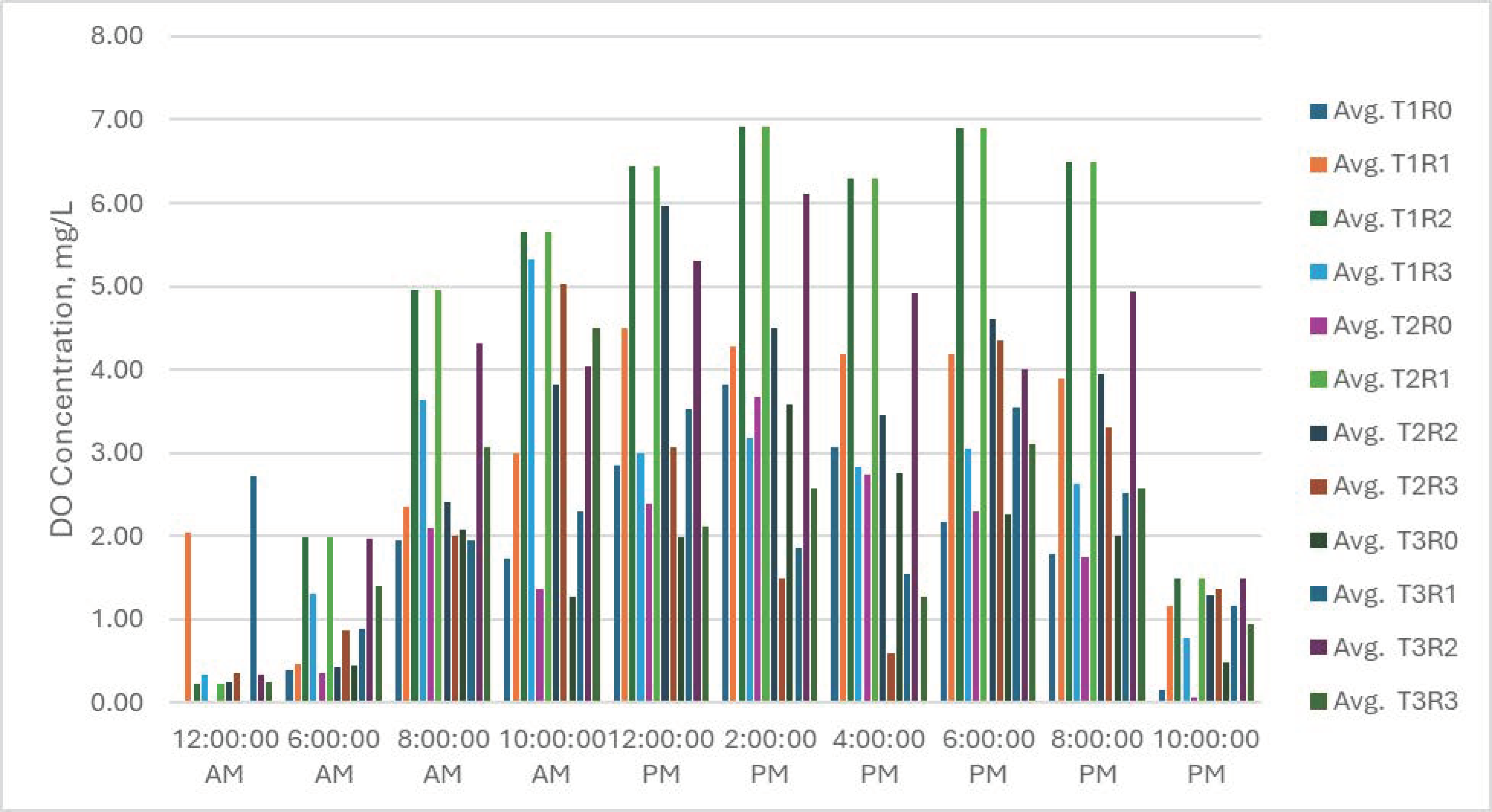
DO was measured at different times during the day. The average DO concentration while the aerators were running was 3.57 mg/L, and it was 1.64 mg/L when the aerators were not running, as summarized in Figure 2.
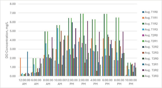
Figure 2.
Dissolved oxygen concentrations at varying times of day.
In typical wastewater treatment plants, the DO concentration should not exceed 0.2 mg/L of dissolved oxygen for the denitrification process [33,34]. Nitrification, however, occurs in concentrations as high as 4 mg/L [34].
A semi-empirical analysis of the oxygen required for wastewater treatment was conducted [35] and then compared to the estimated amount provided by the air compressor. Enough oxygen was estimated to be provided by the aeration system to oxidize all of the COD and ammonia. However, the reactors were not turbulent, so mixing was not optimized, and it is likely that microbial activity was concentrated in the plant rhizosphere [36]. Consequently, it is unclear how much of the oxygen for degradation came from aeration system and plant roots.
4. Conclusions
The results demonstrate that the greenhouse ecosystem with aeration can treat craft beverage wastewater at the design loading. Two reactors in series were needed to remove the COD at the selected design loading, however, all three were needed for TN and phosphorus removal. Not surprisingly, the actual craft beverage wastewaters from small-volume producers had very variable and extreme wastewater COD, TN, and total phosphorus concentrations. The greenhouse ecosystem still substantially reduced these concentrations; however, extreme events will cause disruptions and eventual system failure.
Particularly, COD spikes starve the plants of oxygen resulting in stress and foliage loss. Plants use oxygen for aerobic respiration and if the oxygen is completely depleted for a long enough period of time, the cells will start to die [37]. Further, plant nutrient uptake limitations can occur if the microbial community within the rhizosphere are depleting that available while consuming large quantities of COD [38]. In this research, after the disruption resulting from the high COD in the cidery wastewater, the plants took over two months to recover.
The treatment mechanism is assumed to be, primarily, microbial degradation of COD in the rhizosphere, microbial nitrification/denitrification, plant uptake of nitrogen, and plant uptake and precipitation of phosphorus. However, ethanol may also be removed by volatilization [39]. In natural systems, volatilization at the water-surface interface has a half-life of only five days [40]. However, the surface water interface was quiescent and had plant growth, so conditions were not optimized for volatilization. Ammonia can also volatilize from wastewater at higher pH values under turbulent conditions, which were not the conditions within the reactors.
Based on this research, the size of the greenhouse ecosystem is estimated to be equal to or smaller than a traditional approach, depending on the influent BOD concentration. A nine-day HRT was used for this research, which could have been reduced to under six days for COD removal at the lower concentrations, as only two reactors were required. An aerated lagoon is the most comparable treatment system to the experimental aerated greenhouse ecosystem used in this research. Using a first order partially mixed design model [41], the estimated residents’ times in a completely stirred tank reactor (n = 1) for BOD concentrations of 1100 and 15,000 mg/L are 17 and 277 days, respectively. If the tank was closer to a plug flow configuration (n = 100), the hydraulic retention times for BOD concentrations of 1100 and 15,000 mg/L are nine and 17 days, respectively. For typical craft beverage wastewater (BOD of 2000 mg/L), the aerated greenhouse ecosystem requires approximately 54% less hydraulic retention time than a dispersed plug flow (n = 3) aerated lagoon. In comparison to the cold weather constructed wetland treating winery wastewater [12] with a BOD of 2000 mg/L and the use of only two reactors, the greenhouse ecosystem requires approximately 26% less hydraulic retention time, which is also proportional to required land area. This size reduction is attributed to the higher and optimized microbial growth in the rhizosphere zone.
Although this research proved the concept of using the greenhouse ecosystem, further research on the removal mechanisms, odor control, and optimization are essential. Sizing the greenhouse ecosystem system was achieved using an organic loading value derived from the literature. A better understanding of the impacts of shock organic loads are also essential. Additional design values that account for nitrogen and phosphorus loading would also be useful.
Author Contributions
Conceptualization, C.E.A. and S.I.S.; Methodology, C.E.A. and S.I.S.; Formal analysis, C.E.A. and S.I.S.; Investigation, C.E.A. and S.I.S.; Resources, S.I.S.; Data curation, C.E.A. and S.I.S.; Writing—original draft, C.E.A. and S.I.S.; Writing—review & editing, C.E.A. and S.I.S.; Supervision, C.E.A. and S.I.S.; Project administration, S.I.S.; Funding acquisition, C.E.A. and S.I.S. All authors have read and agreed to the published version of the manuscript.
Funding
The authors would like to thank the Michigan Craft Beverage Council grant number GG 22*1568 for funding.
Institutional Review Board Statement
Not applicable.
Informed Consent Statement
Not applicable.
Data Availability Statement
Data are contained within the article.
Acknowledgments
The authors would like to acknowledge the Michigan State College of Agriculture and Natural Resources Statistics Consulting Center for statistical analysis. The authors would also like to acknowledge the winery, brewery, and cidery that allowed sample collection at their facilities.
Conflicts of Interest
The authors declare no conflicts of interest. The funders had no role in the design of the study; in the collection, analyses, or interpretation of data; in the writing of the manuscript; or in the decision to publish the results.
References
- US EPA. Wastewater Technology Fact Sheet: The Living Machine; US EPA: Cincinnati, OH, USA, 2001.
- Todd, J.; Brown, E.J.; Wells, E. Ecological design applied. Ecol. Eng. 2003, 20, 421–440. [Google Scholar] [CrossRef]
- Western Consortium for Public Health. Total Resource Recovery Project: Final Report; Western Consortium for Public Health: San Diego, CA, USA, 1996. [Google Scholar]
- Austin, D. Final Report on the South Burlington, Vermont, Advanced Ecologically Engineerd System (AEES); Living Technologies, Inc.: Burlington, VT, USA, 2000. [Google Scholar]
- ITRC Wetlands Team. Technical and Regulatory Guidance Document for Constructed Treatment Wetlands; Interstate Technology Regulatory Council: Washington, DC, USA, 2003. [Google Scholar]
- Jin, Z.; Zheng, Y.; Li, X.; Dai, C.; Xu, K.; Bei, K.; Zheng, X.; Zhao, M. Combined process of bio-contact oxidation-constructed wetland for blackwater treatment. Bioresour. Technol. 2020, 316, 123891. [Google Scholar] [CrossRef]
- Jin, Z.; Lv, C.; Zhao, M.; Zhang, Y.; Huang, X.; Bei, K.; Kong, H.; Zheng, X. Black water collected from the septic tank treated with a living machine system: HRT effect and microbial community structure. Chemosphere 2018, 210, 745–752. [Google Scholar] [CrossRef] [PubMed]
- Lansing, S.L.; Martin, J.F. Use of an ecological treatment system (ETS) for removal of nutrients from dairy wastewater. Ecol. Eng. 2006, 28, 235–245. [Google Scholar] [CrossRef]
- Wang, L.K.; Tay, J.-H.; Tay, S.T.L.; Hung, Y.-T. Environmental Bioengineering; Springer: Berlin/Heidelberg, Germany, 2010; Volume 11, Available online: http://www.springer.com/series/7645 (accessed on 6 May 2022).
- Michigan Department of Environmental Quality. Guidance for the Design of Land Treatment Systems Utilized at Wineries; Michigan Department of Environmental Quality: Lansing, MI, USA, 2015.
- DK Publications. The Beer Book: Your Drinking Companion to Over 1,700 Beers; DK Publishing: London, UK, 2014. [Google Scholar]
- Skornia, K.; Safferman, S.I.; Rodriguez-Gonzalez, L.; Ergas, S.J. Treatment of winery wastewater using bench-scale columns simulating vertical flow constructed wetlands with adsorption media. Appl. Sci. 2020, 10, 1063. [Google Scholar] [CrossRef]
- Bakare, B.; Shabangu, K.; Chetty, M. Brewery wastewater treatment using laboratory scale aerobic sequencing batch reactor. S. Afr. J. Chem. Eng. 2017, 24, 128–134. [Google Scholar] [CrossRef]
- Brito, A.G.; Peixoto, J.; Oliveira, J.M.; Oliveira, J.A.; Costa, C.; Nogueira, R.; Rodrigues, A. Brewery and Winery Wastewater Treatment: Some Focal Points of Design and Operation. In Utilization of By-Products and Treatment of Waste in the Food Industry; Springer: Berlin/Heidelberg, Germany, 2007; Volume 3, pp. 1–22. [Google Scholar]
- Li, H.; Liu, F.; Luo, P.; Xie, G.; Xiao, R.; Hu, W.; Peng, J.; Wu, J. Performance of integrated ecological treatment system for decentralized rural wastewater and significance of plant harvest management. Ecol. Eng. 2018, 124, 69–76. [Google Scholar] [CrossRef]
- Worku, A.; Tefera, N.; Kloos, H.; Benor, S. Bioremediation of brewery wastewater using hydroponics planted with vetiver grass in Addis Ababa, Ethiopia. Bioresour. Bioprocess. 2018, 5, 39. [Google Scholar] [CrossRef]
- Tian, L.; Jinzhong, L.; Shenglin, Y.; Zhourong, Y.; Min, Z.; Hainan, K.; Xiangyong, Z. Treatment via the Living Machine system of blackwater collected from septic tanks: Effect of different plant groups in the systems. Environ. Dev. Sustain. 2021, 23, 1964–1975. [Google Scholar] [CrossRef]
- Johnson, M.B.; Mehrvar, M. Winery wastewater management and treatment in the Niagara Region of Ontario, Canada: A review and analysis of current regional practices and treatment performance. Can. J. Chem. Eng. 2020, 98, 5–24. [Google Scholar] [CrossRef]
- Photone. Keep the Guesswork Out of Grow Lighting. Available online: https://growlightmeter.com/ (accessed on 5 March 2024).
- Burgoon, P.S.; DeBusk, T.A.; Reddy, K.R.; Koopman, B. Vegetated Submerged Beds with Artificial Substrates. 1: BOD Removal. J. Environ. Eng. 1991, 117, 394–407. [Google Scholar] [CrossRef]
- Coleman, J.; Hench, K.; Garbutt, K.; Sexstone, A.; Bissonnette, G.; Skousen, J. Treatment of domestic wastewater by three plant species in constructed wetlands. Water Air Soil Pollut. 2001, 128, 283–295. [Google Scholar] [CrossRef]
- Kulshreshtha, N.M.; Verma, V.; Soti, A.; Brighu, U.; Gupta, A.B. Exploring the contribution of plant species in the performance of constructed wetlands for domestic wastewater treatment. Bioresour. Technol. Rep. 2022, 18, 101038. [Google Scholar] [CrossRef]
- Ng, Y.S.; Chan, D.J.C. Phytoremediation capabilities of Spirodela polyrhiza, Salvinia molesta and Lemna sp. in synthetic wastewater: A comparative study. Int. J. Phytoremediation 2018, 20, 1179–1186. [Google Scholar] [CrossRef] [PubMed]
- Melchiors, E.; Freire, F.B. Winery Wastewater Treatment: A Systematic Review of Traditional and Emerging Technologies and Their Efficiencies. Environ. Process. 2023, 10, 1–22. [Google Scholar] [CrossRef]
- HACH. Sension+ 5051T Portable Combination pH Electrode for ‘Dirty’ (Wastewater) Applications. Available online: https://www.hach.com/p-sension-ph-probes-for-portable-meters-with-temperature-compensation/LZW5051T.97.002#optionalaccessory (accessed on 7 November 2023).
- HACH. HQ1130 Portable Dissolved Oxygen Meter with Dissolved Oxygen Electrode, 1 m Cable. Available online: https://www.hach.com/p-portable-meters-hq1130-do1-channel/LEV015.53.11301 (accessed on 7 November 2023).
- Holmes, D.E.; Dang, Y.; Smith, J.A. Nitrogen Cycling during Wastewater Treatment, 1st ed.; Elsevier Inc.: Amsterdam, The Netherlands, 2019; Volume 106. [Google Scholar] [CrossRef]
- Cho, S.; Kambey, C.; Nguyen, V.K. Performance of anammox processes for wastewater treatment: A critical review on effects of operational condi-tions and environmental stresses. Water 2020, 12, 20. [Google Scholar] [CrossRef]
- Full Circle Brewing, Co. What Is an Adjunct in Brewing? Available online: https://www.fullcirclebrewing.com/post/what-is-an-adjunct-in-brewing#:~:text=Inbrewinganadjunctis,it’saddedtotheboil (accessed on 9 November 2023).
- Gebeyehu, A.; Shebeshe, N.; Kloos, H.; Belay, S. Suitability of nutrients removal from brewery wastewater using a hydroponic technology with Typha latifolia. BMC Biotechnol. 2018, 18, 74. [Google Scholar] [CrossRef]
- Scott Laboratories. Complete Guide to Cider Fermentation Nutrition. Available online: https://scottlab.com/complete-guide-to-cider-fermentation-nutrition (accessed on 5 March 2024).
- Wittenham Hill Cidery. Nitrogen—The Forgotten Element in Cider Making. Available online: http://www.cider.org.uk/nitro.htm (accessed on 5 March 2024).
- Hong, P.; Wu, X.; Shu, Y.; Wang, C.; Tian, C.; Gong, S.; Cai, P.; Donde, O.O.; Xiao, B. Denitrification characterization of dissolved oxygen microprofiles in lake surface sediment through analyzing abundance, expression, community composition and enzymatic activities of denitrifier functional genes. AMB Express 2019, 9, 1–10. [Google Scholar] [CrossRef]
- Tchobanoglous, G.; Burton, F.L.; Stensel, D.H. Metcalf&Eddy: Wastewater Engineering: Treatment and Reuse, 5th ed.; no. 7; McGraw-Hill Education; McGraw Hill Companies, Inc.: New York, NY, USA, 2014; pp. 632–639. [Google Scholar]
- Reynolds, T.D.; Richards, P.A. Unit Operations and Processes in Environmental Engineering, 2nd ed.; PWS Publishing Company: Boston, MA, USA, 1996. [Google Scholar]
- Shahid, M.J.; Al-Surhanee, A.A.; Kouadri, F.; Ali, S.; Nawaz, N.; Afzal, M.; Rizwan, M.; Ali, B.; Soliman, M.H. Role of microorganisms in the remediation of wastewater in floating treatmentwetlands: A review. Sustainability 2020, 12, 5559. [Google Scholar] [CrossRef]
- Pucciariello, C.; Perata, P. How plants sense low oxygen. Plant Signal. Behav. 2012, 7, 813–816. [Google Scholar] [CrossRef]
- Zhu, Q.; Riley, W.J.; Tang, J. A new theory of plant–microbe nutrient competition resolves inconsistencies between observations and model predictions. Ecol. Appl. 2017, 27, 875–886. [Google Scholar] [CrossRef] [PubMed]
- Seeger, E.M.; Reiche, N.; Kuschk, P.; Borsdorf, H.; Kaestner, M. Performance evaluation using a three compartment mass balance for the removal of volatile organic compounds in pilot scale constructed wetlands. Environ. Sci. Technol. 2011, 45, 8467–8474. [Google Scholar] [CrossRef] [PubMed]
- Ohio Department of Health: Bureau of Environmental Health and Radiation Protection. Ethanol: Answers to Frequently Asked Health Questions. 2016. Available online: http://www.cdc.gov/niosh/npg (accessed on 26 November 2023).
- US EPA. Principles of Design and Operations of Wastewater Treatment Pond Systems for Plant Operators, Engineers, and Managers; US EPA: Washington, DC, USA, 2011.

Disclaimer/Publisher’s Note: The statements, opinions and data contained in all publications are solely those of the individual author(s) and contributor(s) and not of MDPI and/or the editor(s). MDPI and/or the editor(s) disclaim responsibility for any injury to people or property resulting from any ideas, methods, instructions or products referred to in the content. |
© 2024 by the authors. Licensee MDPI, Basel, Switzerland. This article is an open access article distributed under the terms and conditions of the Creative Commons Attribution (CC BY) license (https://creativecommons.org/licenses/by/4.0/).