The Role of Labor Force, Physical Capital, and Energy Consumption in Shaping Agricultural and Industrial Output in Pakistan

Abstract

The labor force, physical capital, and energy sources are key economic drivers that enhance the output levels of developing economies. Despite their significance, the impact of these factors on agricultural and industrial output in Pakistan remains underexplored. This study aims to address this gap by examining the effects of the labor force, physical capital, and energy consumption—including electricity, oil, and gas—on agricultural and industrial output. Additionally, we explore the combined effects of electricity and oil consumption on these sectors. Based on unit root test results, which indicate that the variables as either I(0) or I(1), the Autoregressive Distributed Lag (ARDL) technique is selected. This method is particularly effective for handling mixed integration orders and provides robust estimates in small sample sizes, allowing for a thorough examination of both short- and long-run dynamics. Using annual time-series data from Pakistan for the period 1990–2022, the empirical results reveal that higher levels of the labor force, physical capital, electricity consumption, oil consumption, and gas consumption significantly increase agricultural and industrial output in both the short and long run. Furthermore, the findings reveal that the combined effect of electricity and oil consumption has a stronger impact on agricultural and industrial output compared to their individual effects. These results are further validated using alternative econometric techniques such as DOLS and FMOLS. To enhance Pakistan’s agricultural and industrial performance, policies should prioritize investment in human capital and physical capital development, ensure reliable and efficient energy supplies, and promote integrated energy management strategies. These steps are crucial for fostering sustainable economic growth and productivity in both sectors.

1. Introduction

Classical and neoclassical theories emphasize the importance of the labor force and physical capital as primary drivers of economic output, with labor force participation influenced by population dynamics and physical capital formation enhancing productivity through investments in machinery and infrastructure [1,2,3]. However, these theories often treat technological advancements as exogenous factors that temporarily offset diminishing returns. In contrast, endogenous growth theories, such as those by Romer and Lucas, highlight the role of human capital, innovation, and technological advancements as internal mechanisms driving sustained growth [4,5,6]. These models emphasize quality over quantity in labor force participation, with education and skill development playing pivotal roles in enhancing productivity and promoting continuous improvements in productivity and economic growth through technological innovation and energy efficiency.

The agricultural and industrial sectors are fundamental to Pakistan’s economic landscape, each significantly contributing to the country’s GDP. In the agricultural sector, labor is a critical component, employing about 40% of the workforce and significantly contributes to 24% of the GDP (https://www.pbs.gov.pk/content/agriculture-statistics (accessed on 19 October 2023)). This sector is characterized by labor-intensive activities, but productivity is often hampered by traditional farming practices, limited access to modern technology, and insufficient education and training for the labor force [7]. Capital investment in agriculture, including expenditures on machinery, irrigation systems, and infrastructure, is essential for enhancing productivity and output. However, farmers frequently encounter difficulties in accessing financial resources and credit, which restricts their ability to modernize and expand their operations [8]. Moreover, energy consumption in the agricultural sector is vital, influencing both direct and indirect activities. Direct energy use includes operating machinery, irrigation systems, and processing agricultural products, while indirect energy consumption involves the production of essential inputs like fertilizers [9]. A reliable and affordable energy supply is crucial for agricultural efficiency and productivity [10]. Energy shortages or high costs can severely disrupt agricultural activities, leading to decreased output and economic instability in Pakistan. Improvements in energy infrastructure and efficiency significantly boost agricultural productivity, emphasizing the need for comprehensive policies that address energy issues alongside labor and capital investments [11].

In the industrial sector, labor productivity is generally higher than in agriculture, primarily due to better access to technology, capital, and training. The industrial sector contributes around 20% of Pakistan’s GDP (https://data.worldbank.org/indicator/NV.IND.TOTL.ZS?locations=PK (accessed on 19 October 2023))and performs a main function in the country’s economic development [12]. Capital investment in this sector includes expenditures on advanced machinery, infrastructure, and human capital, all of which are necessary for maintaining and increasing industrial output. Despite its potential, the industrial sector faces several challenges, including political instability, inadequate infrastructure, and limited access to financial resources, which can impede growth and development [13]. Furthermore, energy consumption is a major determinant of industrial output, as the sector relies heavily on energy for manufacturing processes and the operation of machinery. The availability and cost of energy significantly impact industrial productivity and competitiveness [14]. This underscores the importance of energy efficiency and investment in modern technology. Policies that enhance energy infrastructure, promote energy efficiency, and support the adoption of renewable energy sources are essential for boosting industrial productivity [15].

Energy sources serves as a fundamental input for almost all economic activities; therefore, the global demand for energy is raising day by day. Energy consumption became a main topic particularly after the 1970s’ energy crises which were largely responsible for the continued rise in energy prices [16]. The crisis also highlighted the reliance on oil not only for transportation but also for electricity generation, as oil is a major component in power plants. This raised awareness of the importance of energy diversification, as well as the development of alternative energy sources and technologies. The dramatic rise in oil prices also increased the cost of agricultural production. This was due to rising fuel prices, which are necessary for operating machinery, transporting goods, and producing fertilizers and pesticides [17]. According to the report of the International Energy Agency (IEA), oil, gas, and electricity continue to dominate the global energy landscape, collectively accounting for more than 90% of the projected increase in energy demand. This dominance underscores the critical role these energy sources play in powering economies and supporting industrial and agricultural activities worldwide. The IEA report further highlights the pivotal role of energy as a crucial input in the production function, emphasizing that its contribution to output growth surpasses that of other economic factors. Energy is not merely a component of production but a catalyst for economic expansion, enabling industrial processes, technological advancements, and overall productivity improvements. This dynamic association between energy consumption and economic growth suggests that ensuring a reliable and efficient energy supply is vital for sustaining and enhancing economic development in Pakistan. The report also points to the need for continued investment in energy infrastructure and innovation to meet the rising demand while addressing environmental and sustainability concerns [18].

In recent years, the concept of sustainability has gained prominence in discussions of economic growth and energy use. Sustainability advocates for achieving the same or greater economic output with reduced energy consumption, which is essential in the context of growing environmental concerns and limited natural resources [10]. In particular, this research focuses on Pakistan, a developing economy with unique challenges and opportunities in its pursuit of sustainable growth, and the country’s reliance on traditional energy sources, coupled with its ambitions for rapid industrialization and agricultural expansion. Therefore, this study is framed within this sustainability discussion, exploring the roles of the labor force and physical capital in enhancing sectoral performance and promoting sustainable economic growth through the use of various energy resources. Given the specific economic and industrial context of Pakistan, this research highlights the importance of balancing energy consumption with the need for sustained growth, aligning with global sustainability goals. The preface of sustainability in this discussion provides a contemporary relevance to the study, ensuring that the findings contribute to ongoing debates about how to achieve economic progress without compromising environmental integrity.

Based on the theories of economic growth and the above discussion, it is evident that the enhancement of facilities and structures related to labor, capital, and energy plays a crucial role in boosting the output of both the agriculture and industrial sectors. These factors are significant in shaping the sectoral output within Pakistan’s economy [19]. Understanding how these elements contribute to sectoral performance is vital for developing effective policies and promoting sustainable economic growth. To address this, our study aims to explore several key aspects: Firstly, we investigate the impact of labor force participation on the productivity of the agricultural and industrial sectors in Pakistan. This objective seeks to determine how variations in labor force engagement influence sectoral output. Secondly, we examine the effects of physical capital formation on agricultural and industrial output. This analysis aims to identify how investments in physical infrastructure contribute to enhancing the productivity of agriculture and industry. Thirdly, we analyze the influence of energy consumption—including electricity, oil, and gas—on the productivity of the agricultural and industrial sectors. This objective is designed to assess how different forms of energy contribute to sectoral performance. Lastly, we explore the interaction impact of electricity and oil consumption on agricultural and industrial productivity. By examining the interaction between various energy types, we aim to provide a comprehensive understanding of their collective effect on sectoral output. Through these objectives, the study aims to offer valuable insights for policymakers and stakeholders, aiding in the development of strategies that foster sustainable economic growth and enhance sectoral performance in Pakistan.

2. Literature Review

2.1. The Labor Force, Physical Capital, and Sectoral Output

The labor force and physical capital are foundational drivers of economic growth, particularly in developing economies. For instance, Umair et al. [7] emphasize the crucial role that the labor force plays in Pakistan’s economic activities. Their research investigates the effects of labor force participation on economic growth, particularly highlighting the significance of health and education expenditures. The study’s findings reveal that increased labor force participation significantly enhances economic growth in both the short and long term. This positive impact is further amplified by improved health and education services, stressing the necessity for policies that invest in human capital development.

Supporting this perspective, Ali and Akhtar [20] explore the impact of FDI, research and development, and human capital on total factor productivity (TFP) growth in Pakistan. Their results indicate that both physical and human capitals are the most significant contributors to output growth. The study shows a positive correlation between TFP growth and increases in physical capital, human capital, and FDI, suggesting that strategic investments in these areas are essential for achieving sustainable economic growth. They recommend focusing on human capital as a pivotal element to enhance output growth and TFP in Pakistan. Similarly, Pomi et al. [21] investigate the interaction between human and physical capital in influencing Bangladesh’s economic growth. Their findings indicate that both forms of capital contribute to economic growth over different timeframes, although their efficiencies vary. This aligns with the broader evidence presented by Li et al. [13], who examine the roles of physical, human, and social capital in China’s economic growth. Their empirical analysis confirms that both physical and human capital significantly drive economic growth through capital accumulation and improved labor productivity.

Despite the established importance of labor force participation and physical capital in driving economic growth, there is limited research that specifically examines their combined effects on agricultural and industrial output in Pakistan. This study addresses this gap by investigating how these factors contribute to sectoral output, providing a deeper understanding of their roles in Pakistan’s economy.

Hypothesis 1.

Higher levels of labor force participation positively impact agricultural and industrial output in Pakistan.

Hypothesis 2.

Increased physical capital formation leads to higher agricultural and industrial output in Pakistan.

2.2. Energy Consumption and Sectoral Output

Energy consumption is another critical factor influencing economic growth, particularly in energy-dependent sectors such as agriculture and industry. Abbasi et al. [14] conducted a comprehensive analysis of how energy consumption and industrial growth affect economic growth in Pakistan. Their empirical evidence demonstrates that both electricity consumption and the value added by industry have significant impacts on economic growth in both the short and long term. Based on these findings, the study recommends that economic policy planning should focus on enhancing electricity generation and management. This includes investing in renewable energy sources and banning low-efficiency electrical appliances to improve overall energy efficiency. Supporting this perspective, Fatima et al. [19] investigated the causal relationships between renewable energy generation, overall energy consumption, human capital, and economic performance in Pakistan. Their research confirms a two-way causal relationship between energy use and economic performance, as well as between renewable energy generation and economic performance. These findings support the growth hypothesis, highlighting that both renewable and total energy use are critical for driving economic growth. This suggests that policies promoting renewable energy and efficient energy use are not only environmentally beneficial but also crucial for sustaining economic development.

In their detailed study, Nasir et al. [22] offer an insightful breakdown of how different types of energy consumption influence both industrial and agricultural productivity. Their results show a negative relationship between electricity consumption and industrial output due to power supply failures in developing countries. However, in the agriculture sector, energy consumption positively influences output. Similarly, Umair et al. [23] explored the relationship between various types of energy consumption and industrial output, revealing a significant positive impact in the long run. Specifically, they found that oil, electricity, and gas consumption are strongly linked to increased industrial output. Their study underscores the importance of ensuring a reliable supply of these energy sources to support and sustain industrial growth. The authors highlight the critical need for strategic efforts to address and meet the energy demands of the industrial sector, suggesting that targeted energy policies and investments are essential for fostering long-term industrial development.

In the same context, Rehman and Bashir [24] reveal that the real agricultural output is enhanced by energy consumption and government expenditure, while the labor force and gross fixed capital formation negatively influence agricultural output in the long run. This aligns with the findings of Khan et al. [25], who explored the causal relationship between GDP and energy consumption in Pakistan using a trivariate model that includes capital formation. Their research indicates a bidirectional causal link between GDP and energy consumption, underscoring the interdependence between Pakistan’s energy sector and its economic output. Based on these findings, they advocate for liberalizing the energy sector and implementing reforms to encourage the adoption of renewable energy sources. Similarly, Chandio et al. [11] investigated the connection between energy consumption and agricultural economic growth in Pakistan. Their study revealed that both gas and electricity consumption have a positive impact on agricultural growth. This emphasizes the critical role of energy availability in supporting agricultural productivity and growth in Pakistan. Furthermore, Abokyi et al. [26] delved into the dynamics between electricity consumption and industrial growth in Ghana. The study found that while electricity consumption generally spurs productivity, it negatively impacts manufacturing sector output due to the declining share of industrial sector electricity consumption. This highlights the complexity of the relationship, which varies across different contexts and sectors.

Furthermore, Rastegaripour et al. [27] identified energy usage as a crucial factor in the production processes of both the agricultural and industrial sectors in developing countries. In a similar vein, Ishioro [28] conducted a study in Nigeria that underscored the crucial role of energy consumption in influencing sectoral output. The research identified a positive and significant relationship between energy consumption and the output of various sectors, indicating that higher energy consumption tends to boost sectoral performance. However, the study also presented a nuanced perspective by revealing that, over the long term, the increasing energy consumption could lead to adverse effects on the industrial sector’s performance. This finding suggests that while energy consumption is vital for immediate growth and productivity, there are potential negative consequences that need to be managed to ensure sustainable industrial development. Moreover, Olofin et al. [29] examined the link between disaggregated energy consumption and sectoral output in West African countries. Their findings revealed distinct patterns of correlation. Notably, fossil fuel consumption was negatively correlated with both agricultural and industrial output, suggesting a potential negative impact on productivity. In contrast, electricity consumption was positively correlated with industrial output, underscoring its importance in enhancing industrial productivity and economic growth. Additionally, the study found that diesel consumption was positively associated with industrial output. Mitic et al. [30] examined energy consumption in the agricultural sector across several EU countries. They found that high levels of energy consumption were particularly prevalent in countries with larger agricultural sectors, such as France and Poland.

Previous studies have explored the impact of energy consumption on economic growth; there is a lack of research focusing on its sector-specific effects in Pakistan, particularly the combined impact of different energy types on agricultural and industrial output. This study seeks to fill this gap by analyzing how electricity, oil, and gas consumption influence sectoral output, both individually and in combination.

Hypothesis 3.

Increased energy consumption (electricity, oil, and gas) positively impacts agricultural and industrial output in Pakistan.

Hypothesis 4.

The combined effect of electricity and oil consumption has a stronger impact on agricultural and industrial output compared to their individual effects.

3. Theoretical Framework

The agricultural sector of the developing countries relies heavily on the labor force, capital formation, and energy inputs. In the age of globalization, local industries are increasingly importing new machinery that requires energy-intensive environments. Although the adaptation to new technologies and machinery in the production process is often swift, it results in more efficient and productive agricultural practices [31]. Similarly, in the industrial sector, energy consumption (oil, gas, electricity) is critical for maintaining and increasing output levels [23]. The availability and efficient use of energy resources are essential for operating machinery, manufacturing processes, and overall industrial productivity [32]. These sectors require skilled workers to implement innovations, improve production processes, and capture new markets, thereby driving economic output.

This study is grounded in the Solow growth model [1], which provides a framework for understanding economic output through the interplay of three critical factors: labor, physical capital, and technological advancement. It proposes that economic output can be achieved through the accumulation of labor, physical capital, and technological improvement. The model also emphasizes the importance of domestic and international savings and investments in physical capital formation [1,33]. This perception expands on the previous Harrod–Domar growth model, which focused mainly on physical capital. The Solow growth model expands on this basis by highlight the role of labor, capital, and the knowledge in the production function. We have used energy input as a proxy of technology following by Umair et al. [23]. This is represented in the model as a mathematical equation.

$$Y=f(AL,K)$$

(1)

where Y denotes the output or production level, A represents the total factor productivity or technological efficiency, L stands for the labor force input, and K represents the physical capital input. Equation (1) captures the relationship between the output and the inputs of labor and capital, moderated by technological progress or efficiency.

$$\begin{array}{ll}\therefore K^{\alpha }{(AL)}^{1-\alpha }& \\ Y/AL=[K^{\alpha }.{(AL)}^{1-\alpha }]/AL& \\ Y/AL=K^{\alpha }.{(AL)}^{1-\alpha -1}& \\ Y/AL=K^{\alpha }.{(AL)}^{-\alpha }& \\ Y/AL={(K/AL)}^{\alpha }& \\ \therefore \tilde{y}=Y/AL& \\ \therefore \tilde{k}=K/AL& \\ \mathrm{(2)}& \tilde{y}={(\tilde{k})}^{\alpha }\end{array}$$

where K is the ratio of capital per worker to technology. y is the ratio per output per unit of technology.

$$\begin{array}{ll}\tilde{k}=K/AL& \\ \ln \tilde{k}=\ln K-\ln (AL)& \\ \ln \tilde{k}=\ln K-\ln A-\ln L& \\ \partial \ln \tilde{k}=\partial \ln K-\partial \ln A-\partial \ln L& \\ \partial \ln \tilde{k}/\partial t=\partial \ln K/\partial t-\partial \ln A/\partial t-\partial \ln L/\partial t& \\ 1/\tilde{k}.\partial \tilde{k}/\partial t=1/K.\partial K/\partial t-1/A.\partial A/\partial t-1/L.\partial L/\partial t& \\ \stackrel{•}{\stackrel{~}{k}}/\tilde{k}=\stackrel{•}{K}/K-\stackrel{•}{A}/A-\stackrel{•}{L}/L& \\ \therefore g=\stackrel{•}{A}/A& \\ \therefore n=\stackrel{•}{L}/L& \\ \mathrm{(3)}& \stackrel{•}{\stackrel{~}{k}}/\tilde{k}=\stackrel{•}{K}/K-g-n\end{array}$$

For capital accumulation equation,

$$\begin{array}{ll}\mathrm{(4)}& \stackrel{•}{\stackrel{~}{k}}/\tilde{k}=[(sY-\delta K)/K]-g-n\stackrel{•}{\stackrel{~}{(k}}/\widetilde{k)}.\tilde{k}=(s\tilde{y}/\tilde{k}).\tilde{k}-(n+g+\delta ).\tilde{k}\stackrel{•}{\stackrel{~}{k}}/\tilde{k}=(sY/K-\delta K/K)-g-n& \\ \stackrel{•}{\stackrel{~}{k}}/\tilde{k}=(sY/K)-\delta -g-n& \\ \stackrel{•}{\stackrel{~}{k}}/\tilde{k}=(sY/K)-(n+g+\delta )& \\ \stackrel{•}{\stackrel{~}{k}}/\tilde{k}=(sY/AL)/(K/AL)-(n+g+\delta )& \\ \stackrel{•}{\stackrel{~}{k}}/\tilde{k}=(s\tilde{y}/\tilde{k})-(n+g+\delta )& \\ \stackrel{•}{\stackrel{~}{k}}/\tilde{k}=[(sY-\delta K)/K]-g-n& \end{array}$$

Hence, the Solow equation is

$$\stackrel{•}{\stackrel{~}{k}}=s\tilde{y}-(n+g+\delta ).\tilde{k}$$

(5)

where $\stackrel{•}{\stackrel{~}{k}}$ is the growth rate of capital or change in capital per worker and $\tilde{y}$ is the output per worker, while $s\tilde{y}$ is the amount of output generated through new capital based on savings and investment. $s$ is the rate that is reinvested into the economy from the total output to build more capital. $(n+g+\delta ).\tilde{k}$ shows the rate at which the capital per worker diminishes, i.e., due to population enhancement, technological improvement, and depreciation where capital becomes obsolete over time. For the steady-state growth path, $\stackrel{•}{\stackrel{~}{k}}$ i = 0, then $s\tilde{y}$ = $(n+g+\delta ).\tilde{k}$. This means that the actual level of investment matches the breakeven level of investment in this occurrence.

The Solow growth model advocates for an open market system as it fosters trade, which in turn boosts domestic resources and savings. An open market also attracts foreign investment, which introduces new technologies and ideas that boost labor force efficiency, especially in developing countries. The new technology and innovation improves the manufacturing process, while the integration of physical and human capital mitigates the impact of declining marginal returns. As a result, the Solow growth theory emphasizes the critical role of human capital development, emphasizing the value of a labor force and innovative ideas. The expanded model is reformulated as follows:

$$Y=A{L}^{\Phi }{K}^{{\rm B}}$$

(6)

$$Y=A{L}^{\Phi }{K}^{{\rm B}}X{i}^{\Upsilon }$$

$$lnY=\ln A+\Phi \ln L+{\rm B}\ln K+\Upsilon \ln Xi+u$$

(7)

In Equation (7), $Y$ is the proxy of the output level, where $A$ denotes the total factor productivity which includes the energy input. Likewise, $K$ is the amount of capital and $Xi$ represents the control variables. Furthermore, $\Phi$, ${\rm B}$, $\Upsilon$ are the production elasticities. $u$ represents the error term. Basically, Equation (7) indicates the log linear form of the model.

4. Materials and Methods

4.1. Data

We analyze annual time-series data from Pakistan spanning the years 1990 to 2022. The variables we examine include agricultural output (AO), labor in agriculture (LBA), capital in agriculture (CPA), electricity consumption in agriculture (ELA), oil consumption in agriculture (OILA), and gas consumption in agriculture (GSA). For the industrial sector, we include industrial output (IO), labor in industry (LABI), capital in industry (CPI), electricity consumption in industry (ELI), oil consumption in industry (OILI), and gas consumption in industry (GSI). Additionally, we consider inflation (INF) and trade openness (OPN) as control variables. Detailed information about these variables is provided in

Table 1. Variables, description, and sources.

Variables	Description	Signs	Source
Dependent variables
Agricultural Output (AO)	Log of agricultural value added (constant LCU in millions)		WDI, World Bank
Industrial Output (IO)	Log of industrial value added (constant LCU in millions)		WDI, World Bank
Core variables
Labor in Agriculture (LBA)	Log of number of labor working in agricultural sector (millions)	+	PBS
Capital in Agriculture (CPA)	Log of capital use in agricultural sector (constant LCU in millions)	+	PBS
Electricity Consumption in Agriculture (ELA)	Log of electricity consumption in agricultural sector (Gwh)	+	PBS
Oil Consumption in Agriculture (OILA)	Log of oil consumption in agricultural sector (tons)	+	PBS
Gas Consumption in Agriculture (GSA)	Log of gas consumption in agricultural sector (mm cft)	+	PBS
Labor in Industry (LABI)	Log of number of labor working in industrial sector (million)	+	PBS
Capital in Industry (CPI)	Log of capital use in industrial sector (constant LCU in millions)	+	PBS
Electricity Consumption in Industry (ELI)	Log of electricity consumption in industrial sector (Gwh)	+	PBS
Oil Consumption in Industry (OILI)	Log of oil consumption in industrial sector (tons)	+	PBS
Gas Consumption in Industry (GSI)	Log of gas consumption in industrial sector (mm cft)	+	PBS
Control variables
Inflation (INF)	Consumer price index (2010 = 100)	−	WDI, World Bank
Trade Openness (OPN)	Trade openness (% of GDP)	+	WDI, World Bank

Notes: WDI denotes the World Development Indicator; PBS denotes Pakistan Bureau of Statistics.

.

4.2. Methods and Model Specifications

This study delves into the relationships and causality between variables using the Auto Regressive Distributed Lag (ARDL) technique and an Error Correction Model (ECM). We chose the ARDL model due to its proven effectiveness in examining dynamic associations, as highlighted by influential studies such as those by Pesaran and Shin [34], Pesaran et al. [35], and Narayan [36]. The ARDL approach is particularly suited for our analysis because it allows for the simultaneous assessment of both short-term dynamics and long-term relationships. This dual capability is crucial for understanding the complex interactions between the labor force, physical capital, energy consumption, and agricultural and industrial growth over time. The ARDL bounds testing method, developed by Pesaran et al. [35], further enables us to investigate the existence of long-term relationships while considering potential short-term fluctuations. One of the significant advantages of the ARDL model is its flexibility in handling variables with different orders of integration, such as levels I(0) and first differences I(1). This means we can include both stationary and non-stationary variables within the same model, which is a common scenario in economic and social science research. According to Narayan [36], the ARDL estimation technique is renowned for producing robust and consistent results even with small sample sizes, enhancing the reliability of our findings.

To further validate the robustness of our empirical models, we perform an extensive robustness analysis employing the Dynamic Ordinary Least Squares (DOLS) and Fully Modified Ordinary Least Squares (FMOLS) techniques. By examining the relationships among the variables through these alternative methodologies, we reinforced the reliability and consistency of our findings, providing a more comprehensive perspective on the results. Our empirical models are outlined below:

• Model 1:

$$AO={\phi }_0+{\phi }_{1}LBA+{\phi }_{2}CPA+{\phi }_{3}ECA+{\phi }_{4}INF+{\phi }_{5}OPN+{\mu }_t$$

(8)

where AO represents agricultural output, LBA denotes labor in agriculture, CPA signifies capital in agriculture, ECA stands for energy consumption in agriculture, INF indicates the inflation rate, and OPN represents trade openness. To measure energy consumption, we use three proxies: oil (OILA), electricity (ELA), and gas (GSA) consumption in the agricultural sector. Therefore, Equation (8) is reformulated as follows:

$$AO={\phi }_0+{\phi }_{1}LBA+{\phi }_{2}CPA+{\phi }_{3}OILA+{\phi }_{4}ELA+{\phi }_{5}GSA+{\phi }_{6}INF+{\phi }_{7}OPN+{\mu }_t$$

(9)

Model 2:

We extend the Model 1 by incorporating the interaction between oil consumption and electricity consumption within the agriculture sector (OILA × ELA).

$$AO={\phi }_0+{\phi }_{1}LBA+{\phi }_{2}CPA+{\phi }_{3}OILA+{\phi }_{4}ELA+{\phi }_{5}GSA+{\phi }_{6}OILA\times ELA+{\phi }_{7}INF+{\phi }_{8}OPN+{\mu }_t$$

(10)

Model 3:

$$IO={\phi }_0+{\phi }_{1}LBI+{\phi }_{2}CPI+{\phi }_{3}ECI+{\phi }_{4}INF+{\phi }_{5}OPN+{\mu }_t$$

(11)

where IO represents industrial output, LBI denotes labor in industry, CPI stands for capital in industry, and ECI stands for energy consumption in industry. We utilize three proxies for energy consumption: oil (OILI), electricity (ELI), and gas (GSI) consumption in industrial sector. Therefore, Equation (11) is reformulated as follows:

$$IO={\phi }_0+{\phi }_{1}LBI+{\phi }_{2}CPI+{\phi }_{3}OILI+{\phi }_{4}ELI+{\phi }_{5}GSI+{\phi }_{6}INF+{\phi }_{7}OPN+{\mu }_t$$

(12)

Model 4:

We extend Model 3 by incorporating the interaction between oil consumption and electricity consumption within the industry sector (OILI × ELI).

$$IO={\phi }_0+{\phi }_{1}LBI+{\phi }_{2}CPI+{\phi }_{3}OILI+{\phi }_{4}ELI+{\phi }_{5}GSI+{\phi }_{6}OILI\times ELI+{\phi }_{7}INF+{\phi }_{8}OPN+{\mu }_t$$

(13)

Now, we reformulate all the four models into the ARDL framework. This transformation allows for the incorporation of both short and long-run dynamics between the variables, making it a versatile tool for analyzing the relationships within the data. The ARDL models are expressed as follows:

• ARDL Framework of Model 1:

$$\begin{gathered} \Delta A{O}_t={\alpha }_0+{\alpha }_{1}LB{A}_{t-1}+{\alpha }_{2}CP{A}_{t-1}+{\alpha }_{3}OIL{A}_{t-1}+{\alpha }_{4}EL{A}_{t-1}+ \\ {\alpha }_{5}GAS{A}_{t-1}+{\alpha }_{6}FR{T}_{t-1}+{\alpha }_{7}CR{D}_{t-1}+{\displaystyle \sum _{i=1}^{\mathcal{l}}{\beta }_{1}A{O}_{t-i}}+ \\ {\displaystyle \sum _{\upsilon =0}^{\mathcal{l}}{\beta }_{2}LB{A}_{t-\upsilon }}+{\displaystyle \sum _{\nu =0}^{\mathcal{l}}{\beta }_{3}CP{A}_{t-\nu }}+{\displaystyle \sum _{\omega =0}^{\mathcal{l}}{\beta }_4\Delta OIL{A}_{t-\omega }}+ \\ \hspace{1em}\hspace{1em}\hspace{1em}\hspace{1em}\hspace{1em}\hspace{1em}\hspace{1em}\hspace{1em}\hspace{1em}\hspace{1em}\hspace{1em}\hspace{1em}\hspace{1em}\hspace{1em}\hspace{1em}\hspace{1em}\hspace{1em}\hspace{1em}\hspace{1em}{\displaystyle \sum _{\tau =0}^{\mathcal{l}}{\beta }_5\Delta EL{A}_{\tau -0}}+{\displaystyle \sum _{\psi =0}^{\mathcal{l}}{\beta }_6\Delta GS{A}_{t-\psi }}+{\displaystyle \sum _{\pi =0}^{\mathcal{l}}{\beta }_7\Delta IN{F}_{t-\pi }}+{\displaystyle \sum _{\sigma =0}^{\mathcal{l}}{\beta }_8\Delta OP{N}_{t-\sigma }}+e_t \end{gathered}$$

(14)

The long-run parameters are presented in Equation (15) as follows:

$$\begin{array}{r}A{O}_t={\delta }_0+{\displaystyle \sum _{i=1}^{\mathcal{l}}{\delta }_{1i}A{O}_{t-i}}+{\displaystyle \sum _{\upsilon =0}^{\mathcal{l}}{\delta }_{2i}LB{A}_{t-\upsilon }}+{\displaystyle \sum _{\nu =0}^{\mathcal{l}}{\delta }_{3i}CP{A}_{t-\nu }}+\\ {\displaystyle \sum _{\omega =0}^{\mathcal{l}}{\delta }_{4i}OIL{A}_{t-\omega }}+{\displaystyle \sum _{\tau =0}^{\mathcal{l}}{\delta }_{5i}EL{A}_{\tau -0}}+{\displaystyle \sum _{\psi =0}^{\mathcal{l}}{\delta }_{6i}GS{A}_{t-\psi }}+\\ {\displaystyle \sum _{\pi =0}^{\mathcal{l}}{\delta }_{7i}IN{F}_{t-\pi }}+{\displaystyle \sum _{\sigma =0}^{\mathcal{l}}{\delta }_{8i}OP{N}_{t-\sigma }}+e_t\end{array}$$

(15)

The short-run parameters are displayed in Equation (16) as follows:

$$\begin{array}{r}\Delta A{O}_t={\delta }_0+{\displaystyle \sum _{i=1}^{\mathcal{l}}{\delta }_{1i}\Delta A{O}_{t-i}}+{\displaystyle \sum _{\upsilon =0}^{\mathcal{l}}{\delta }_{2i}\Delta LB{A}_{t-\upsilon }}+{\displaystyle \sum _{\nu =0}^{\mathcal{l}}{\delta }_{3i}\Delta CP{A}_{t-\nu }}+\\ {\displaystyle \sum _{\omega =0}^{\mathcal{l}}{\delta }_{4i}\Delta OIL{A}_{t-\omega }}+{\displaystyle \sum _{\tau =0}^{\mathcal{l}}{\delta }_{5i}\Delta EL{A}_{\tau -0}}+{\displaystyle \sum _{\psi =0}^{\mathcal{l}}{\delta }_{6i}\Delta GS{A}_{t-\psi }}+\\ {\displaystyle \sum _{\pi =0}^{\mathcal{l}}{\delta }_{7i}\Delta IN{F}_{t-\pi }}+{\displaystyle \sum _{\sigma =0}^{\mathcal{l}}{\delta }_{8i}\Delta OP{N}_{t-\sigma }}+\varphi EC{M}_{t-1}+e_t\end{array}$$

(16)

ARDL Framework of Model 2:

$$\begin{gathered} \Delta A{O}_t={\alpha }_0+{\alpha }_{1}LB{A}_{t-1}+{\alpha }_{2}CP{A}_{t-1}+{\alpha }_{3}OIL{A}_{t-1}+{\alpha }_{4}EL{A}_{t-1}+ \\ {\alpha }_{5}GAS{A}_{t-1}+{\alpha }_{6}OILA\times EL{A}_{t-1}+{\alpha }_{7}IN{F}_{t-1}+{\alpha }_{8}OP{N}_{t-1} \\ +{\displaystyle \sum _{i=1}^{\mathcal{l}}{\beta }_1\Delta A{O}_{t-i}}+{\displaystyle \sum _{\upsilon =0}^{\mathcal{l}}{\beta }_2\Delta LB{A}_{t-\upsilon }}+{\displaystyle \sum _{\nu =0}^{\mathcal{l}}{\beta }_3\Delta CP{A}_{t-\nu }}+\hspace{1em}\hspace{1em}\hspace{1em}\hspace{1em}\hspace{1em}\hspace{1em}\hspace{1em}\hspace{1em}\hspace{1em}\hspace{1em} \\ {\displaystyle \sum _{\omega =0}^{\mathcal{l}}{\beta }_4\Delta OIL{A}_{t-\omega }}+{\displaystyle \sum _{\tau =0}^{\mathcal{l}}{\beta }_5\Delta EL{A}_{\tau -\tau }}+{\displaystyle \sum _{\psi =0}^{\mathcal{l}}{\beta }_6\Delta GS{A}_{t-\psi }}+ \\ {\displaystyle \sum _{\zeta =0}^{\mathcal{l}}{\beta }_7\Delta }OILA\ast EL{A}_{t-\zeta }+{\displaystyle \sum _{\pi =0}^{\mathcal{l}}{\beta }_8\Delta IN{F}_{t-\pi }}+{\displaystyle \sum _{\sigma =0}^{\mathcal{l}}{\beta }_9\Delta OP{N}_{t-\sigma }}+e_t \end{gathered}$$

(17)

The long-run parameters are presented in Equation (18) as follows:

$$\begin{gathered} A{O}_t={\delta }_0+{\displaystyle \sum _{i=1}^{\mathcal{l}}{\delta }_{1i}A{O}_{t-i}}+{\displaystyle \sum _{\upsilon =0}^{\mathcal{l}}{\delta }_{2i}LB{A}_{t-\upsilon }}+{\displaystyle \sum _{\nu =0}^{\mathcal{l}}{\delta }_{3i}CP{A}_{t-\nu }}+\hspace{1em}\hspace{1em} \\ {\displaystyle \sum _{\omega =0}^{\mathcal{l}}{\delta }_{4i}OIL{A}_{t-\omega }}+{\displaystyle \sum _{\tau =0}^{\mathcal{l}}{\delta }_{5i}EL{A}_{\tau -\tau }}+{\displaystyle \sum _{\psi =0}^{\mathcal{l}}{\delta }_{6i}GS{A}_{t-\psi }}+\hspace{1em}\hspace{1em} \hspace{1em} \\ {\displaystyle \sum _{\zeta =0}^{\mathcal{l}}{\delta }_{7i}OILA\ast EL{A}_{\zeta -0}}+{\displaystyle \sum _{\pi =0}^{\mathcal{l}}{\delta }_{8i}IN{F}_{t-\pi }}+{\displaystyle \sum _{\sigma =0}^{\mathcal{l}}{\delta }_{9i}OP{N}_{t-\sigma }}+e_t \end{gathered}$$

(18)

The short-run parameters are shown in Equation (19) as follows:

$$\begin{array}{l}\Delta A{O}_t={\delta }_0+{\displaystyle \sum _{i=1}^{\mathcal{l}}{\delta }_{1i}\Delta A{O}_{t-i}}+{\displaystyle \sum _{\upsilon =0}^{\mathcal{l}}{\delta }_{2i}\Delta LB{A}_{t-\upsilon }}+{\displaystyle \sum _{\nu =0}^{\mathcal{l}}{\delta }_{3i}\Delta CP{A}_{t-\nu }}+\\ \hspace{1em}{\displaystyle \sum _{\omega =0}^{\mathcal{l}}{\delta }_{4i}\Delta OIL{A}_{t-\omega }}+{\displaystyle \sum _{\tau =0}^{\mathcal{l}}{\delta }_{5i}\Delta EL{A}_{\tau -\tau }}+{\displaystyle \sum _{\psi =0}^{\mathcal{l}}{\delta }_{6i}\Delta GS{A}_{t-\psi }}+\\ \hspace{1em}{\displaystyle \sum _{\zeta =0}^{\mathcal{l}}{\delta }_{7i}\Delta OILA\ast EL{A}_{\zeta -0}}+{\displaystyle \sum _{\pi =0}^{\mathcal{l}}{\delta }_{8i}\Delta IN{F}_{t-\pi }}+{\displaystyle \sum _{\sigma =0}^{\mathcal{l}}{\delta }_{9i}\Delta OP{N}_{t-\sigma }}+\varphi EC{M}_{t-1}+e_t\end{array}$$

(19)

ARDL Framework of Model 3:

$$\begin{gathered} \Delta I{O}_t={\alpha }_0+{\alpha }_{1}LB{I}_{t-1}+{\alpha }_{2}CP{I}_{t-1}+{\alpha }_{3}OIL{I}_{t-1}+{\alpha }_{4}EL{I}_{t-1}+{\alpha }_{5}GS{I}_{t-1}+ \\ {\alpha }_{6}IN{F}_{t-1}+{\alpha }_{7}OP{N}_{t-1}+{\displaystyle \sum _{i=1}^{\mathcal{l}}{\beta }_{1}I{O}_{t-i}}+{\displaystyle \sum _{\upsilon =0}^{\mathcal{l}}{\beta }_{2}LB{I}_{t-\upsilon }}+ \\ {\displaystyle \sum _{\nu =0}^{\mathcal{l}}{\beta }_{3}CP{I}_{t-\nu }}+{\displaystyle \sum _{\omega =0}^{\mathcal{l}}{\beta }_4\Delta OIL{I}_{t-\omega }}+{\displaystyle \sum _{\tau =0}^{\mathcal{l}}{\beta }_5\Delta EL{I}_{\tau -\tau }}+ \\ {\displaystyle \sum _{\psi =0}^{\mathcal{l}}{\beta }_6\Delta GS{I}_{t-\psi }}+{\displaystyle \sum _{\pi =0}^{\mathcal{l}}{\beta }_7\Delta IN{F}_{t-\pi }}+{\displaystyle \sum _{\sigma =0}^{\mathcal{l}}{\beta }_8\Delta OP{N}_{t-\sigma }}+e_t \end{gathered}$$

(20)

The long-run parameters are presented in Equation (21) as follows:

$$\begin{gathered} I{O}_t={\delta }_0+{\displaystyle \sum _{i=1}^{\mathcal{l}}{\delta }_{1i}I{O}_{t-i}}+{\displaystyle \sum _{\upsilon =0}^{\mathcal{l}}{\delta }_{2i}LB{I}_{t-\upsilon }}+{\displaystyle \sum _{\nu =0}^{\mathcal{l}}{\delta }_{3i}CP{I}_{t-\nu }}+{\displaystyle \sum _{\omega =0}^{\mathcal{l}}{\delta }_{4i}OIL{I}_{t-\omega }} \\ \hspace{1em}\hspace{1em}\hspace{1em}\hspace{1em}\hspace{1em}\hspace{1em}\hspace{1em}\hspace{1em}\hspace{1em}\hspace{1em}\hspace{1em}\hspace{1em}\hspace{1em}+{\displaystyle \sum _{\tau =0}^{\mathcal{l}}{\delta }_{5i}EL{I}_{\tau -0}}+{\displaystyle \sum _{\psi =0}^{\mathcal{l}}{\delta }_{6i}GS{I}_{t-\psi }}+{\displaystyle \sum _{\pi =0}^{\mathcal{l}}{\delta }_{7i}IN{F}_{t-\pi }}+{\displaystyle \sum _{\sigma =0}^{\mathcal{l}}{\delta }_{8i}OP{N}_{t-\sigma }}+e_t \end{gathered}$$

(21)

The short-run parameters are shown in Equation (22) as follows:

$$\begin{gathered} \Delta I{O}_t={\delta }_0+{\displaystyle \sum _{i=1}^{\mathcal{l}}{\delta }_{1i}\Delta I{O}_{t-i}}+{\displaystyle \sum _{\upsilon =0}^{\mathcal{l}}{\delta }_{2i}\Delta LB{I}_{t-\upsilon }}+{\displaystyle \sum _{\nu =0}^{\mathcal{l}}{\delta }_{3i}\Delta CP{I}_{t-\nu }}+{\displaystyle \sum _{\omega =0}^{\mathcal{l}}{\delta }_{4i}\Delta OIL{I}_{t-\omega }} \\ +{\displaystyle \sum _{\tau =0}^{\mathcal{l}}{\delta }_{5i}EL{I}_{\tau -0}}+{\displaystyle \sum _{\psi =0}^{\mathcal{l}}{\delta }_{6i}\Delta GS{I}_{t-\psi }}+{\displaystyle \sum _{\pi =0}^{\mathcal{l}}{\delta }_{7i}\Delta IN{F}_{t-\pi }}+\hspace{1em}\hspace{1em}\hspace{1em} \hspace{1em}\hspace{1em}\hspace{1em} \\ {\displaystyle \sum _{\sigma =0}^{\mathcal{l}}{\delta }_{8i}\Delta OP{N}_{t-\sigma }}+\varphi EC{M}_{t-1}+e_t\hspace{1em}\hspace{1em}\hspace{1em}\hspace{1em}\hspace{1em}\hspace{1em}\hspace{1em}\hspace{1em}\hspace{1em}\hspace{1em}\hspace{1em}\hspace{1em}\hspace{1em}\hspace{1em}\hspace{1em}\hspace{1em} \end{gathered}$$

(22)

ARDL Framework of Model 4:

$$\begin{gathered} \Delta I{O}_t={\alpha }_0+{\alpha }_{1}LB{I}_{t-1}+{\alpha }_{2}CP{I}_{t-1}+{\alpha }_{3}OIL{I}_{t-1}+{\alpha }_{4}EL{I}_{t-1}+{\alpha }_{5}GS{I}_{t-1}+ \\ {\alpha }_{6}OILI\ast EL{I}_{t-1}+{\alpha }_{7}IN{F}_{t-1}+{\alpha }_{8}OP{N}_{t-1}+{\displaystyle \sum _{i=1}^{\mathcal{l}}{\beta }_1\Delta I{O}_{t-i}}+ \\ {\displaystyle \sum _{\upsilon =0}^{\mathcal{l}}{\beta }_2\Delta LB{I}_{t-\upsilon }}+{\displaystyle \sum _{i=\nu }^{\mathcal{l}}{\beta }_3\Delta CP{I}_{t-\nu }}+{\displaystyle \sum _{i=\omega }^{\mathcal{l}}{\beta }_4\Delta OIL{I}_{t-\omega }}+ \\ {\displaystyle \sum _{\tau =0}^{\mathcal{l}}{\beta }_5\Delta EL{I}_{\tau -0}}+{\displaystyle \sum _{\psi =0}^{\mathcal{l}}{\beta }_6\Delta GS{I}_{t-\psi }}+{\displaystyle \sum _{\zeta =0}^{\mathcal{l}}{\beta }_7\Delta }OILI\ast EL{I}_{t-\zeta }+\hspace{1em}\hspace{1em}\hspace{1em}\hspace{1em}\hspace{1em}\hspace{1em}\hspace{1em} \\ \hspace{1em}\hspace{1em}\hspace{1em}\hspace{1em}\hspace{1em}\hspace{1em}\hspace{1em}\hspace{1em}\hspace{1em}\hspace{1em}\hspace{1em}\hspace{1em}\hspace{1em}\hspace{1em}{\displaystyle \sum _{\pi =0}^{\mathcal{l}}{\beta }_8\Delta IN{F}_{t-\pi }}+{\displaystyle \sum _{\sigma =0}^{\mathcal{l}}{\beta }_9\Delta OP{N}_{t-\sigma }}+e_t \end{gathered}$$

(23)

The long-run parameters are displayed in Equation (24) as follows:

$$\begin{gathered} I{O}_t={\delta }_0+{\displaystyle \sum _{i=1}^{\mathcal{l}}{\delta }_{1i}I{O}_{t-i}}+{\displaystyle \sum _{\upsilon =0}^{\mathcal{l}}{\delta }_{2i}LB{I}_{t-\upsilon }}+{\displaystyle \sum _{\nu =0}^{\mathcal{l}}{\delta }_{3i}CP{I}_{t-\nu }}+ \\ \hspace{1em}\hspace{1em}\hspace{1em}\hspace{1em}\hspace{1em}{\displaystyle \sum _{\omega =0}^{\mathcal{l}}{\delta }_{4i}OIL{I}_{t-\omega }}+{\displaystyle \sum _{\tau =0}^{\mathcal{l}}{\delta }_{5i}EL{I}_{\tau -\tau }}+{\displaystyle \sum _{\psi =0}^{\mathcal{l}}{\delta }_{6i}GS{I}_{t-\psi }}+ \\ \hspace{1em}\hspace{1em}\hspace{1em}\hspace{1em}\hspace{1em}\hspace{1em}\hspace{1em}\hspace{1em}\hspace{1em}\hspace{1em}\hspace{1em}\hspace{1em}\hspace{1em}\hspace{1em}\hspace{1em}\hspace{1em}\hspace{1em}{\displaystyle \sum _{\zeta =0}^{\mathcal{l}}{\delta }_{7i}OILI\ast EL{I}_{\zeta -0}}+{\displaystyle \sum _{\pi =0}^{\mathcal{l}}{\delta }_{8i}IN{F}_{t-\pi }}+{\displaystyle \sum _{\pi =0}^{\mathcal{l}}{\delta }_{9i}OP{N}_{t-\pi }}+e_t \end{gathered}$$

(24)

The short-run parameters are presented in Equation (25) as follows:

$$\begin{gathered} \Delta I{O}_t={\delta }_0+{\displaystyle \sum _{i=1}^{\mathcal{l}}{\delta }_{1i}\Delta I{O}_{t-i}}+{\displaystyle \sum _{\upsilon =0}^{\mathcal{l}}{\delta }_{2i}\Delta LB{I}_{t-\upsilon }}+{\displaystyle \sum _{\nu =0}^{\mathcal{l}}{\delta }_{3i}\Delta CP{I}_{t-\nu }}+ \\ \hspace{1em}\hspace{1em}\hspace{1em}\hspace{1em}\hspace{1em}\hspace{1em}{\displaystyle \sum _{\omega =0}^{\mathcal{l}}{\delta }_{4i}\Delta OIL{I}_{t-\omega }}+{\displaystyle \sum _{\tau =0}^{\mathcal{l}}{\delta }_{5i}\Delta EL{I}_{\tau -\tau }}+{\displaystyle \sum _{\psi =0}^{\mathcal{l}}{\delta }_{6i}\Delta GS{I}_{t-\psi }}+ \\ \hspace{1em}\hspace{1em}\hspace{1em}\hspace{1em}\hspace{1em}\hspace{1em}\hspace{1em}\hspace{1em}\hspace{1em}\hspace{1em}\hspace{1em}\hspace{1em}\hspace{1em}\hspace{1em}\hspace{1em}\hspace{1em}\hspace{1em}\hspace{1em}{\displaystyle \sum _{\zeta =0}^{\mathcal{l}}{\delta }_{7i}\Delta OILI\ast EL{I}_{\zeta -0}}+{\displaystyle \sum _{\pi =0}^{\mathcal{l}}{\delta }_{8i}\Delta IN{F}_{t-\pi }}+{\displaystyle \sum _{\pi =0}^{\mathcal{l}}{\delta }_{9i}\Delta OP{N}_{t-\pi }}+\varphi EC{M}_{t-1}+e_t \end{gathered}$$

(25)

5. Results

5.1. Descriptive Statistics

The statistics presented in

Table 2. Descriptive statistics.

Variables	AO	IO	LBA	CPA	OILA	ELA	GSA	LBI	CPI	OILI	ELI	GSI	INF	OPN
Mean	15.54	15.13	3.00	11.62	11.25	8.91	12.15	17.76	13.13	14.24	9.81	12.16	4.22	0.24
Median	15.59	15.21	3.02	11.81	11.48	8.98	12.17	17.78	13.40	14.28	9.89	12.31	4.10	0.14
Std. Dev.	0.28	0.45	0.21	1.47	1.22	0.22	0.25	0.28	0.94	0.25	0.31	0.44	0.77	0.22
Skewness	−0.34	−0.12	−0.20	−0.07	−0.31	−0.42	−0.74	−0.21	−0.37	−0.25	−0.17	−0.39	0.02	0.86
Kurtosis	2.03	1.63	1.46	1.52	1.49	2.00	2.97	1.74	1.97	2.20	1.53	1.62	1.80	2.56
Jarque-Bera	1.92	2.65	3.48	3.03	3.69	2.34	3.05	2.43	2.20	1.23	3.14	3.44	1.97	4.37
Probability	0.38	0.27	0.18	0.22	0.16	0.31	0.22	0.30	0.33	0.54	0.21	0.18	0.37	0.11
Maximum	15.99	15.82	3.26	13.73	12.64	9.22	12.53	18.18	14.37	14.70	10.27	12.72	5.57	0.73
Minimum	14.99	14.38	2.64	9.36	9.45	8.42	11.53	17.32	11.23	13.78	9.33	11.39	2.89	0.03
Observations	33	33	33	33	33	33	33	33	33	33	33	33	33	33

provide an insightful overview of the central tendencies and variability of key economic indicators related to the agricultural and industrial sectors. The mean and median values indicate that the data points for most variables are centrally clustered, showing a general trend and typical value for each indicator. For instance, the means of agricultural output (AO) and industrial output (IO) are 15.54 and 15.13, respectively, highlighting the relative scale and productivity levels in these sectors. The standard deviation values reveal that certain indicators, such as capital in agriculture (CPA) and oil consumption in agriculture (OILA), exhibit higher variability, suggesting they are more susceptible to fluctuations compared to other variables like labor in agriculture (LBA) and electricity consumption in agriculture (ELA), which are more stable.

Moreover, the skewness and kurtosis values provide insights into the distribution shape of these economic indicators. Most variables exhibit a skewness close to zero, indicating a relatively symmetrical distribution, although some like gas consumption in agriculture (GSA) show a noticeable negative skewness, suggesting a left-tailed distribution. The kurtosis values are generally below three, indicating a flatter distribution than the normal distribution. The Jarque–Bera test probabilities support the hypothesis that most variables follow a normal distribution, with values close to one further affirming this. Overall, these statistics suggest a balanced mix of stability and variability among the economic indicators, with some indicators demonstrating significant fluctuations that could impact the agricultural and industrial sectors differently.

5.2. Correlation Matrix and Variance Inflation Factor

The correlation matrix results in

Table 3. Correlation matrix.

Variables	AO	IO	LBA	CPA	OILA	ELA	GSA	LBI	CPI	OILI	ELI	GSI	INF	OPN
AO	1
IO	0.74	1
LBA	0.67	0.66	1
CPA	0.76	0.67	0.56	1
OILA	0.57	0.75	−0.62	−0.66	1
ELA	0.58	0.77	0.61	0.78	−0.77	1
GSA	0.73	0.74	0.60	0.62	−0.75	0.67	1
LBI	0.67	0.69	0.56	0.69	−0.84	0.83	0.70	1
CPI	0.45	0.69	0.64	0.78	−0.81	0.83	0.76	0.78	1
OILI	0.31	0.36	−0.42	−0.39	0.31	−0.41	−0.18	−0.36	−0.29	1
ELI	0.67	0.78	0.53	0.78	−0.74	0.86	0.70	0.67	0.87	−0.40	1
GSI	0.87	0.65	0.85	0.55	−0.73	0.80	0.83	0.74	0.86	−0.44	0.86	1
INF	−0.82	−0.78	0.66	0.58	−0.85	0.82	0.83	0.79	0.87	−0.30	0.75	0.78	1
OPN	0.75	0.81	0.57	0.72	−0.63	0.80	0.69	0.70	0.86	−0.37	0.88	0.60	0.83	1

reveal significant insights into the relationships between the key variables. There is a strong positive correlation between labor in agriculture (LBA), capital in agriculture (CPA), and energy consumption in agriculture (ELA, GSA, OILA) and agricultural output (AO). Similarly, there is a strong positive correlation between labor in industry (LBI), capital in industry (CPI), and energy consumption in industry (ELI, GSI, OILI) and industrial output (IO). This suggests that increases in labor and capital investments, as well as energy consumption, are associated with higher agricultural and industrial productivity. Additionally, inflation (INF) shows a strong negative correlation with both agricultural and industrial outputs, indicating that higher inflation rates may hinder economic productivity. Trade openness (OPN) generally shows positive correlations, suggesting that greater integration into the global market positively impacts both agricultural and industrial outputs.

The estimates in

Table 4. Variance Inflation Factor.

Variables	VIF	1/VIF
LBA	2.10	0.47
CPA	3.12	0.32
OILA	1.03	0.97
ELA	0.62	1.61
GSA	2.13	0.47
LBI	3.32	0.30
CPI	3.76	0.27
OILI	1.23	0.81
ELI	2.53	0.39
GSI	1.28	0.78
INF	2.10	0.48
OPN	0.33	3.03

signify that there is no multicollinearity in the models, as all Variance Inflation Factor (VIF) values are well below the commonly accepted threshold of 10. Specifically, the VIF values range from 0.33 (for OPN) to 3.76 (for CPI), suggesting that none of the independent variables are highly correlated with each other. This is further supported by the 1/VIF values, which are all above 0.1, reinforcing the absence of multicollinearity. Therefore, the model’s estimates are reliable, and the variables can be interpreted independently without concern for inflated standard errors.

5.3. Unit Root Analysis

To ensure the reliability of our time-series data, we utilized several stationarity tests: the Kwiatkowski–Phillips–Schmidt–Shin (KPSS) test, the Dickey–Fuller Generalized Least Squares (DF-GLS) test, and the Ng–Perron test. These tests are standard tools in econometric analysis, crucial for determining whether data are stationary or if they exhibit a trend over time. The results of these tests are presented in

Table 5. Unit root results.

Variables	Level			1st Difference
	KPSS	DF-GLS	Ng-Perron	KPSS	DF-GLS	Ng-Perron
IO	<0.1	>0.1	>0.1	<0.01	<0.01	>0.01
AO	<0.1	>0.1	>0.1	<0.05	<0.01	<0.05
LBA	>0.05	<0.1	<0.05	>0.1	>0.01	>0.01
CPA	>0.05	>0.1	>0.1	<0.05	<0.01	<0.01
OILA	>0.1	<0.05	<0.05	<0.01	<0.05	<0.01
ELA	<0.05	>0.1	>0.1	>0.1	<0.01	<0.01
GSA	>0.05	>0.1	>0.05	>0.1	>0.05	<0.01
LBI	>0.05	>0.1	>0.1	>0.1	<0.01	<0.05
CPI	<0.01	>0.1	>0.1	>0.1	<0.01	<0.01
OILI	>0.1	<0.01	>0.1	<0.05	<0.01	<0.01
ELI	<0.05	>0.1	>0.1	>0.1	<0.01	<0.01
GSI	<0.05	>0.1	>0.1	<0.01	<0.01	<0.01
INF	>0.05	>0.1	>0.1	>0.1	<0.05	<0.05
OPN	>0.05	>0.1	>0.1	>0.1	<0.01	<0.01

Notes: All the variables are estimated at intercept and trend.

, which lists the p-values for each variable tested. The findings indicate that certain variables, including LBA, CPA, OILA, GSA, INF, OPN, LBI, and OILI are stationary at their levels, denoted as I(0). This suggests that these variables do not show a trend in their original form, making them suitable for direct analysis. On the other hand, variables such as AO, IO, ELA, ELI, and CPI are stationary only after first differencing, indicated as I(1). This means that these variables exhibit a trend in their raw data form, and differencing is necessary to remove this trend and achieve stationarity.

In this condition, the ARDL model is well-suited for estimating variables of different integration orders (both I(0) and I(1)) within a unified regression framework. By analyzing long-term relationships between variables, considering their varying levels of stationarity, the ARDL model proves effective in examining economic data.

5.4. Regression Analysis

In the regression analysis, we first test the long-run relationship before applying the ARDL technique. The bound test results, presented in

Table 6. Bound test estimates of ARDL.

		Model 1		Model 2		Model 3		Model 4
Test-Stat	Significant	I(0)	I(1)	I(0)	I(1)	I(0)	I(1)	I(0)	I(1)
	1%	2.73	3.9	2.62	3.77	2.73	3.9	2.62	3.77
	5%	2.17	3.21	2.11	3.15	2.17	3.21	2.11	3.15
	10%	1.92	2.89	1.85	2.85	1.92	2.89	1.85	2.85
F-stat		9.64		7.92		9.83		8.80
k		7		8		7		8

, indicate a strong long-run relationship among the variables, evidenced by F-statistics significantly exceeding the critical values at all conventional levels of significance (1%, 5%, and 10%). Specifically, the F-statistics of 9.64, 7.92, 9.83, and 8.80 across the four models decisively reject the null hypothesis of no cointegration, indicating robust statistical evidence that the variables move together over the long run despite short-term fluctuations. This establishes the presence of cointegration, which justifies the application of the ARDL technique for further analysis.

The long-run results from the ARDL models are presented in

Table 7. Long-run ARDL estimates of agricultural output.

Dep. Var: Agricultural Output	Model 1	Model 2
LBA	0.516 ***	0.496 ***
	(0.182)	(0.139)
CPA	0.165 ***	0.421 ***
	(0.032)	(0.121)
OILA	0.137 *	0.165 ***
	(0.076)	(0.033)
ELA	0.333 ***	0.848 ***
	(0.08)	(0.182)
GSA	0.049 **	0.592 ***
	(0.02)	(0.171)
OILA × ELA		1.184 **
		(0.495)
INF	−0.341	−0.349 ***
	(0.094)	(0.123)
OPN	0.502 ***	1.277 **
	(0.149)	(0.623)
C	5.857 ***	8.598 ***
	(1.107)	(1.011)

Notes: Standard errors are indicated in (); significance levels are denoted by ***, **, and * denote 1%, 5%, and 10%, respectively.

and

Table 8. Long-run ARDL estimates of industrial output.

Dep. Var: Industrial Output	Model 3	Model 4
LBI	0.156	0.396 **
	(0.102)	(0.165)
CPI	0.126 ***	0.205 ***
	(0.022)	(0.022)
OILI	0.037 **	0.749 **
	(0.019)	(0.290)
ELI	0.002 ***	0.479 ***
	(0.001)	(0.102)
GSI	0.296 ***	0.186 ***
	(0.037)	(0.038)
OILI × ELI		1.269 ***
		(0.618)
INF	−0.035	0.249 ***
	(0.078)	(0.058)
OPN	0.110	0.322 ***
	(0.089)	(0.063)
C	9.047 ***	10.743 ***
	(0.696)	(2.464)

Notes: Standard errors are indicated in (); significance levels are denoted by ***and ** denote 1% and 5% respectively.

. Table 7 focuses on agricultural output (AO) as the dependent variable, with labor in agriculture (LBA), capital in agriculture (CPA), oil consumption in agriculture (OILA), electricity consumption in agriculture (ELA), gas consumption in agriculture (GSA), inflation (INF), and trade openness (OPN) as independent variables. Models 1 and 2 explore these relationships, with Model 2 incorporating an interaction term between oil and electricity consumption in agriculture (OILA × ELA). Similarly, Table 8 presents the long-run estimates for industrial output (IO) as the dependent variable, with labor in industry (LBI), capital in industry (CPI), oil consumption in industry (OILI), electricity consumption in industry (ELI), gas consumption in industry (GSI), inflation (INF), and trade openness (OPN) as the independent variables. Models 3 and 4 explore these relationships, with Model 4 introducing the interaction between oil and electricity consumption in industry (OILI × ELI).

Labor in agriculture (LBA) shows consistently positive and significant effects on agricultural output across both models, reinforcing its pivotal role in driving agricultural productivity (Model 1: β = 0.516, p < 0.001; Model 2: β = 0.496, p < 0.001). Similarly, labor in industry (LBI) shows a significant positive effect on industrial output in Model 4 (β = 0.396, p < 0.01). These findings align with previous studies by Potapov [37], Arfah [38], Ali and Akhtar [20], and Umair et al. [7], which also highlight the favorable impact of the labor force on sectoral output.

Physical capital is another critical factor influencing sectoral output in Pakistan. Physical capital in agriculture (CPA) exhibits significant positive effects on agricultural output in both models, underscoring its importance in agricultural performance (Model 1: β = 0.165, p < 0.001; Model 2: β = 0.421, p < 0.001). Similarly, physical capital in industry (CPI) demonstrates consistently positive effects in both models of industrial output (Model 3: β = 0.126, p < 0.001; Model 4: β = 0.205, p < 0.001). These results underscore the pivotal role of capital investment in driving both agricultural and industrial output, consistent with the findings of Li et al. [13], Ikpesu and Okpe [39], Khan et al. [25], and Ali and Akhtar [20].

The coefficient of oil consumption (OILA and OILI) in both sectors highlights its significance in driving sectoral output. The positive and significant coefficients of OILA in agriculture (Model 1: β = 0.137, p < 0.1; Model 2: β = 0.165, p < 0.001) and OILI in industry (Model 3: β = 0.037, p < 0.05; Model 4: β = 0.749, p < 0.05) indicate that increased oil consumption contributes substantially to output growth in these sectors. These results are in line with the studies by Ayeomoni et al. [40] and Rokicki et al. [41], which also emphasize the importance of oil consumption in enhancing sectoral productivity. Similarly, electricity consumption (ELA and ELI) demonstrates a significant positive impact on output in both sectors. The coefficients of ELA in agriculture (Model 1: β = 0.333, p < 0.001; Model 2: β = 0.848, p < 0.001) and ELI in industry (Model 3: β = 0.002, p < 0.001; Model 4: β = 0.479, p < 0.001) reveal that increased electricity consumption leads to higher output levels, reinforcing the importance of reliable energy supply for economic growth. These findings are consistent with the work of Dogan et al. [9], Tapsın [42], Abokyi et al. [26], and Umair et al. [23].

Furthermore, gas consumption (GSA and GSI) also shows a favorable impact on sectoral output, with significant positive coefficients in both the agricultural (Model 1: β = 0.049, p < 0.05; Model 2: β = 0.592, p < 0.001) and industrial (Model 3: β = 0.296, p < 0.001; Model 4: β = 0.186, p < 0.001) models. The results suggest that increased gas consumption is associated with higher output levels, aligning with studies by Mesagan and Adenuga [43], Shaari et al. [44], and Umair et al. [23].

The interaction terms in Models 2 and 4 further highlight the interplay between energy inputs and sectoral output. In agriculture, the interaction between oil and electricity consumption (OILA × ELA) shows a significant positive impact on output (Model 2: β = 1.184, p < 0.001), suggesting that these energy inputs work synergistically to enhance agricultural productivity. Similarly, the coefficient of OILI*ELI (Model 4: β = 1.269, p < 0.001), the interaction between oil and electricity consumption in industry, underscores their combined importance in driving industrial output.

The variable inflation (INF) represents the impact of inflation on the industry and agriculture sectors. A negative coefficient for both sectors indicates that any increase in inflation causes industrial and agricultural activity to decline. However, the agriculture sector’s coefficient is noticeably larger and statistically significant, indicating that agricultural output is more sensitive to changes in inflation than the industry sector. This implies that inflationary pressures may disproportionately affect the agricultural sector, potentially raising input costs and decreasing profitability. Inflationary pressures may raise input costs for farmers (such as fuel, fertilizers, and equipment), resulting in lower profitability and agricultural productivity. The results are same with the study of Soliman et al. [45].

The short-run ARDL estimations for the agricultural and industrial sectors, presented in

Table 9. Short-run ARDL estimates of agricultural output.

Dep. Var: Agricultural Output	Model 1	Model 2
Constant	12.041 ***	13.916 **
	(2.766)	(5.976)
D(AO(−1))	−0.355 **	−0.087
	(0.137)	(0.043)
D(LBA)	0.119 **	0.171 ***
	(0.051)	(0.033)
D(CPA)	0.196 ***	0.049 ***
	(0.012)	(0.012)
D(CPA(−1))	0.12 ***	0.180 ***
	(0.018)	(0.012)
D(OILA)	0.135 ***	0.154
	(0.018)	(0.227)
D(OILA(−1))	0.154 ***	2.639 ***
	(0.017)	(0.251)
D(ELA)	0.268 ***	0.438 ***
	(0.02)	(0.037)
D(ELA(−1))	0.292 ***	0.551
	(0.021)	(0.041)
D(GSA)	0.118 ***	−0.042 *
	(0.006)	(0.019)
D(GSA(−1))	0.046 ***	2.041 ***
	(0.006)	(0.188)
D(OILA × ELA)		2.489 ***
		(0.167)
D(OILA × ELA(−1))		2.143 ***
		(0.143)
D(INF)	0.066 *	0.142 **
	(0.035)	(0.045)
D(INF(−1))	−0.456 ***	−1.119 ***
	(0.101)	(0.105)
D(OPN)	−0.052	1.320 ***
	(0.082)	(0.075)
D(OPN(−1))	−0.314 ***	1.137 ***
	(0.096)	(0.066)
ECM(−1) *	−0.311 ***	−2.191 ***
	(0.059)	(0.082)

Notes: Standard errors are indicated in (); ***, **, and * denote 1%, 5%, and 10%, respectively.

and

Table 10. Short-run ARDL estimates of industrial output.

Dep. Var: Industrial Output	Model 3	Model 4
Constant	13.799 ***	48.204 ***
	(3.194)	(15.666)
D(IO(−1))	0.661 ***	0.529 ***
	(0.139)	(0.068)
D(LI)	0.027	1.841 ***
	(0.055)	(0.175)
D(LI(−1))	0.401 ***	1.083 ***
	(0.066)	(0.146)
D(CPI)	0.074 ***	0.096 ***
	(0.022)	(0.014)
D(CPI(−1))	0.085 ***	0.109 ***
	(0.026)	(0.015)
D(OILI)	0.064 ***	0.551
	(0.012)	(0.321)
D(OILI(−1))	0.074 ***	0.129 ***
	(0.015)	(0.028)
D(ELI)	0.541 ***	0.749 ***
	(0.068)	(0.065)
D(ELI(−1))	0.172 **	0.310
	(0.066)	(0.070)
D(GSI)	0.281 ***	0.332 ***
	(0.029)	(0.019)
D(GSI(−1))	0.236 ***	0.104 ***
	(0.055)	(0.019)
D(OILI × ELI)		10.743 ***
		(0.816)
D(OILI × ELI(−1))		7.519 ***
		(0.574)
D(INF)	−0.002 ***	−0.310 ***
	(0.001)	(0.070)
D(OPN)	0.207 ***	0.027
	(0.057)	(0.029)
D(OPN(−1))	0.328 ***	−0.334 ***
	(0.068)	(0.048)
ECM(−1) *	−2.462 ***	−2.045 ***
	(0.254)	(0.107)

Notes: Standard errors are indicated in (); ***, **, and * denote 1%, 5%, and 10%, respectively.

respectively, reveal the dynamic nature of the models. The primary variables—labor, capital, oil, electricity, and gas—consistently demonstrate a significant relationship with agricultural output, suggesting that investments in these factors positively influence agricultural production in the short run.

Furthermore, Model 2 highlights a fascinating interaction effect between oil and electricity (OILA × ELA) in the agricultural sector, indicating that their combined influence enhances their substantial contributions to agricultural output. Similarly, Model 3 shows that labor, capital, oil, electricity, and gas maintain a significant and positive relationship with industrial output, underscoring the beneficial impact of investing in these resources on industrial productivity in the short run. Additionally, Model 4 illustrates the impactful interaction between oil and electricity on industrial output in the short run, further enhancing production levels in the industry sector.

The coefficient of the Error Correction Model (ECM) term (−1) is a key indicator of how quickly variables adjust back to their long-run equilibrium following a short-run disturbance. A larger ECM coefficient (−1) value indicates a more rapid adjustment process, reflecting the economic system’s resilience and ability to adapt to external shocks. In the first model, the ECM coefficient indicates an annual convergence rate of 31.1%, suggesting that economic growth aligns with the equilibrium path in approximately three years. The second model’s ECM coefficient, significant at the 1% level, shows an annual adjustment rate of 219.1%, implying a very rapid convergence towards long-run equilibrium in less than six months. The third model reveals an annual adjustment rate of approximately 246.2%, indicating an even faster adjustment process where the system overshoots and corrects in less than six months. Likewise, the fourth model shows an annual adjustment rate of approximately 204.5%, suggesting a similarly rapid correction to equilibrium within about six months. These findings collectively demonstrate the models’ ability to quickly adjust back to long-run equilibrium following short-run shocks, underscoring the system’s resilience.

5.5. Robustness Analysis

To further solidify the credibility of our findings, we conducted a robustness analysis using both the Dynamic Ordinary Least Squares (DOLS) and Fully Modified Ordinary Least Squares (FMOLS) methods. These approaches allow us to cross-verify the results obtained from the Autoregressive Distributed Lag (ARDL) model, ensuring that our conclusions are not model-dependent. The results presented in

Table 11. DOLS and FMOLS estimates of agricultural output.

Dep. Var: Agricultural Output	DOLS		FMOLS
	Model 1	Model 2	Model 1	Model 2
LBA	0.178 *	0.157 *	0.335 ***	0.301 **
	(0.091)	(0.088)	(0.030)	(0.066)
CPA	0.134 ***	0.131 ***	0.418 **	0.302 ***
	(0.020)	(0.020)	(0.146)	(0.029)
OILA	0.066 ***	0.279 ***	0.487 ***	1.515 ***
	(0.015)	(0.057)	(0.075)	(0.131)
ELA	0.082 *	0.296 *	1.542 ***	1.518 ***
	(0.044)	(0.127)	(0.132)	(0.130)
GSA	0.144 ***	0.349 **	0.149 ***	0.248 ***
	(0.019)	(0.046)	(0.049)	(0.080)
OILA × ELA		1.624 ***		2.054 **
		(0.367)		(0.811)
INF	−0.104	−0.164 **	−0.057	−0.274
	(0.100)	(0.079)	(0.155)	(0.131)
OPN	0.290 **	0.131	2.815 ***	0.166
	(0.048)	(0.583)	(0.583)	(0.094)
C	3.598 ***	7.029 *	3.397 ***	9.492 *
	(0.861)	(1.654)	(0.777)	(4.597)

Notes: Standard errors are indicated in (); ***, **, and * denote 1%, 5%, and 10%, respectively.

and

Table 12. DOLS and FMOLS estimates of industrial output.

Dep. Var: Industrial Output	DOLS		FMOLS
	Model 3	Model 4	Model 3	Model 4
LBI	0.477 ***	0.276 **	0.477 ***	0.285 **
	(0.090)	(0.136)	(0.090)	(0.436)
CPI	0.200 ***	0.158 ***	0.200 ***	0.269 ***
	(0.017)	(0.025)	(0.017)	(0.066)
OILI	1.934 ***	0.327 ***	1.934 ***	1.767 **
	(0.421)	(0.048)	(0.421)	(0.874)
ELI	1.358 ***	0.319 ***	1.854 ***	0.738 ***
	(0.283)	(0.034)	(0.326)	(0.147)
GSI	0.196 ***	0.193 ***	0.196 ***	0.315 ***
	(0.015)	(0.024)	(0.015)	(0.045)
OILI × ELI		2.113 **		2.854 ***
		(1.006)		(0.626)
INF	−0.203 ***	−0.194 ***	0.048	−0.365
	(0.032)	(0.042)	(0.030)	(1.743)
OPN	0.335 ***	0.203 ***	0.005	0.124
	(0.030)	(0.032)	(0.019)	(0.152)
C	9.736 *	6.443 ***	9.963 *	7.622 **
	(5.614)	(2.290)	(6.918)	(3.109)

Notes: Standard errors are indicated in (); ***, **, and * denote 1%, 5%, and 10%, respectively.

demonstrate a consistency between the long-run coefficients derived from ARDL and those obtained through DOLS and FMOLS. This alignment underscores the robustness and reliability of our analysis.

The robustness analysis highlights that key factors—labor force participation, physical capital, and energy consumption (oil, gas, and electricity)—consistently exhibit a significant and positive impact on both agricultural and industrial outputs. Importantly, the interaction terms between oil and electricity, particularly in the agricultural sector (OILA × ELA) and the industrial sector (OILI × ELI), contribute significantly to output growth. These results suggest that the synergistic use of energy resources, when combined with an increased labor force and capital investment, leads to more robust and sustained growth in these sectors.

These findings underscore the importance of investing in both human and physical capital in Pakistan. It is essential to prioritize investments in infrastructure and energy segment alongside initiatives that enhance the labor force. Policymakers can foster long-term economic output in both the sectors by developing a skilled and motivated workforce while modernizing physical infrastructure and optimizing energy use. The empirical evidence strongly indicates that unlocking Pakistan’s economic potential will depend on these integrated efforts.

5.6. Diagnostic Tests

To ensure the accuracy and reliability of our long-run estimates, we conducted several diagnostic tests: the Ramsey RESET test, White’s test, the Breusch–Pagan–Godfrey test, the Durbin–Watson test, the Serial Correlation LM test, and the normality test. The results, detailed in

Table 13. Diagnostic tests.

Tests	Model 1		Model 2		Model 3		Model 4
	Test-Stat	Prob.	Test-Stat	Prob.	Test-Stat	Prob.	Test-Stat	Prob.
Serial Correlation LM	1.184	0.369	8.546	0.105	1.109	0.364	14.721	0.064
Durbin–Watson	1.978	-	1.981	-	2.170	-	2.458	-
White’s test	0.794	0.685	0.714	0.755	2.376	0.142	2.529	0.046
Breusch–Pagan–Godfrey	0.630	0.812	1.407	0.408	1.361	0.284	0.330	0.965
Normality Test	0.317	0.853	1.216	0.544	1.803	0.406	1.954	0.376
Ramsey RESET Test	0.034	0.866	0.119	0.741	0.259	0.800	0.683	0.508

, demonstrate that none of the four models exhibit any significant issues. Specifically, the Durbin–Watson and Serial Correlation LM tests confirm the absence of autocorrelation, indicating that the errors in our models are not correlated over time. Additionally, both the Breusch–Pagan–Godfrey test and White’s test reveal no signs of heteroskedasticity, suggesting that the variability of the errors is consistent across observations. Finally, the normality test supports the models’ robustness by showing that the residuals follow a normal distribution, which is crucial for the validity of our estimates. Overall, these diagnostic tests reinforce the reliability and soundness of our models.

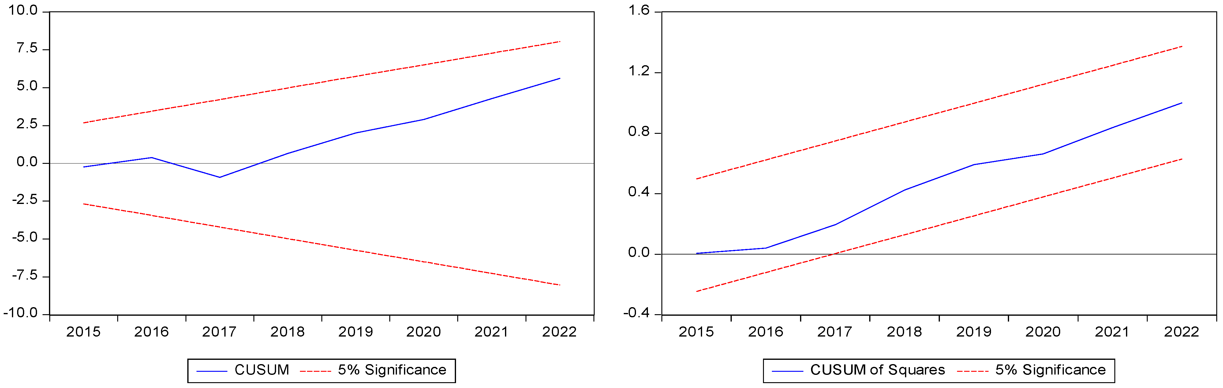
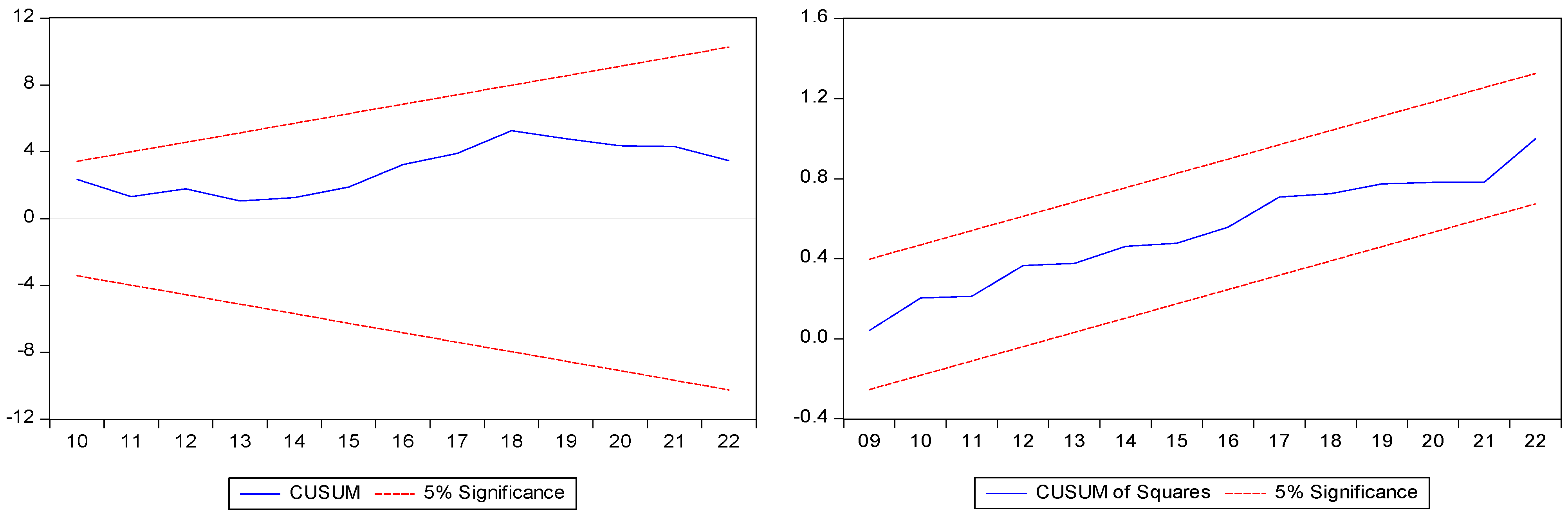
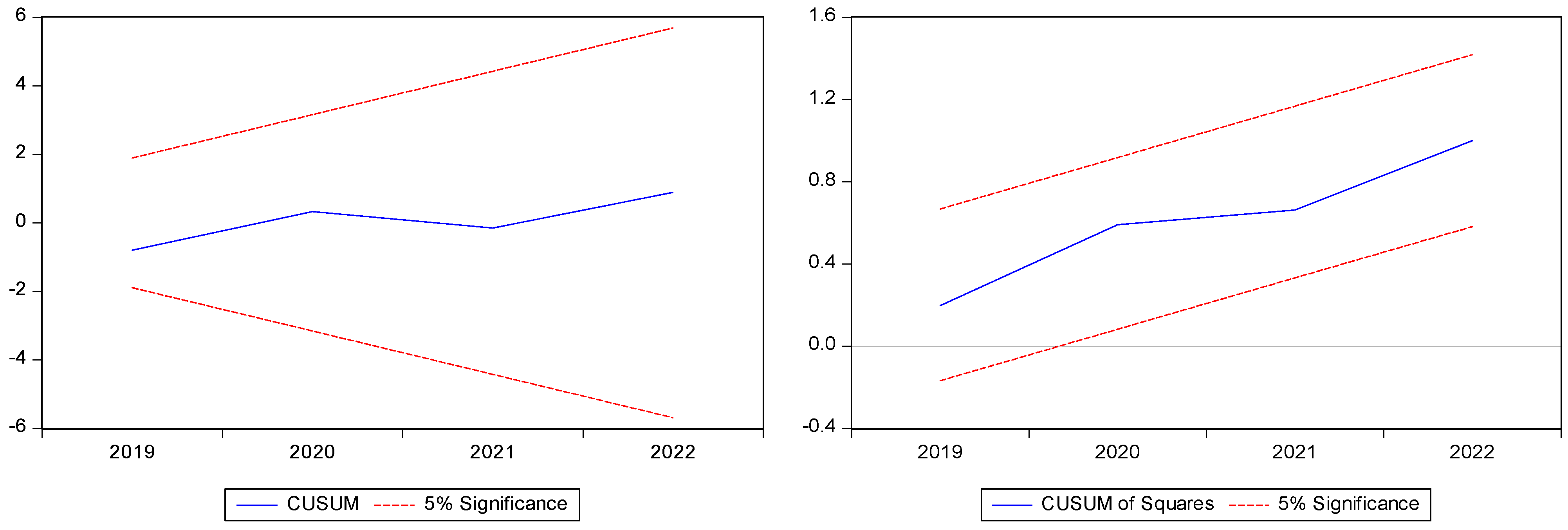
5.7. Stability Estimates

When assessing the stability of a model in the short run, two key tests stand out: the Cumulative Sum (CUSUM) test and the Cumulative Sum of Squares (CUSUMSQ) test. These tools are crucial for understanding how well our model holds up over time. The CUSUM test focuses on tracking the stability of regression coefficients, checking whether they remain consistent throughout the analysis period. In contrast, the CUSUMSQ test takes a broader view, evaluating whether the variability of these coefficients stays steady as time progresses. Together, these tests help to ensure that our model’s results are reliable and robust, as demonstrated by Brown et al. [46].

The analysis has shown that all four models maintain stability with a high level of confidence, specifically within a 5% interval. This stability is clearly depicted in Figure 1, Figure 2, Figure 3 and Figure 4, which visually underscore the reliability and robustness of the models over the short run. These findings not only confirm the models’ soundness but also establish a solid basis for their use in making predictions and applying them effectively within the given context. The consistent stability across models reassures us of their validity and enhances their utility in decision-making processes.

6. Discussion

The findings of this study underscore the critical role of various factors—the labor force, physical capital, and energy consumption—in driving the output of Pakistan’s industrial and agricultural sectors. By analyzing these components, this study reveals the multifaceted ways in which they contribute to economic productivity and offers insights into the potential for sustainable growth.

6.1. The Role of the Labor Force and Physical Capital

The positive impact of the labor force on industrial output highlights the significance of a skilled and motivated workforce in driving productivity. As more individuals enter the labor market, they bring valuable skills and expertise, not only boosting current production levels but also fostering a culture of innovation and efficiency within industries [38]. This cultural shift is crucial for sustained growth and competitiveness in the industrial sector. Similarly, an active and skilled agricultural workforce is essential for managing crops, livestock, and modern farming techniques. Their contribution goes beyond immediate agricultural activities, playing a vital role in ensuring food security, rural development, and sustainable agricultural practices [7]. Thus, the labor force is integral to both sectors, driving growth, innovation, and long-term prosperity.

The significant positive effects of physical capital, as evidenced by the coefficients of CPI and CPA across all models, highlight its crucial role in enhancing productivity. Investment in physical capital—such as machinery, equipment, and infrastructure—directly correlates with increased production capacity, efficiency, and innovation in both industrial and agricultural sectors [13]. These findings suggest that higher levels of capital investment enable these sectors to expand operations, meet growing demand, and improve competitiveness, ultimately contributing to overall economic performance. Physical capital not only facilitates immediate productivity gains but also establishes a foundation for sustained economic development.

6.2. The Role of Energy Consumption: Oil, Electricity, and Gas

The analysis of energy consumption further underscores its pivotal role in both industrial and agricultural output. The positive and significant impact of oil consumption on industrial output (OILI) reflects its importance as a source of energy and raw material for various industrial processes. Oil powers machinery, fuels vehicles, and supports the logistics necessary for efficient production [40]. Similarly, oil consumption in agriculture (OILA) is crucial, powering essential farming machinery and supporting irrigation, fertilization, and pesticide application, all of which are vital for high agricultural productivity [43]. Electricity consumption also plays a significant role in both sectors. The positive effects of electricity input on industrial output (ELI) emphasize its importance in powering machinery and ensuring the smooth operation of manufacturing processes [26]. In agriculture, electricity supports irrigation systems, storage facilities, and processing equipment, leading to higher output levels [9]. Furthermore, gas consumption, as indicated by the significant coefficients for both industrial and agricultural sectors, further highlights its importance. In industry, natural gas is a primary energy source, valued for its cost-effectiveness and reliability, which enables continuous and efficient production [44]. In agriculture, natural gas is a key feedstock for fertilizer production, which directly influences crop yields and overall agricultural output [43].

The interaction between oil and electricity consumption, in both agriculture (OILA × ELA) and industry (OILI × ELI), reveals the synergistic effects of these energy sources on the output. In agriculture, the combined use of oil-powered machinery and electric irrigation systems optimizes production processes, reducing costs and enhancing crop yields. In industry, the integration of oil and electricity facilitates efficient energy utilization and technological advancements, leading to higher productivity and sustainable growth.

6.3. Sustainability and Economic Growth

The discussion section delves into the sustainability implications of the study’s findings. Traditional economic growth models often rely heavily on increased energy consumption. However, this study suggests significant potential to achieve similar or even greater levels of output through more efficient use of the labor force and physical capital. In Pakistan, where energy resources are both vital and costly, sustainability becomes crucial. This study emphasizes that by optimizing investments in the labor force and physical capital, it is possible to decouple economic growth from energy consumption—a necessary step for reducing environmental impact and achieving long-term economic sustainability. The advantages of reduced energy use are manifold. Economically, it leads to lower production costs and increased competitiveness in global markets. Environmentally, it contributes to the reduction in greenhouse gas emissions, aligning with international climate goals. Socially, it fosters more resilient economies, less vulnerable to energy price fluctuations.

However, transitioning to sustainable energy practices presents challenges. It requires a rethinking of current economic models and investments in new technologies and training programs that enhance labor force efficiency and physical capital productivity. This discussion also highlights the need for supportive policy frameworks, including incentives for energy efficiency and the development of renewable energy sources. By situating these findings within the specific context of Pakistan, this discussion provides a nuanced understanding of how sustainability can be integrated into economic growth strategies. The implications are far-reaching, offering a roadmap for other developing countries facing similar challenges.

7. Conclusions and Policy Recommendations

This study comprehensively examined the impact of the labor force, physical capital, and energy consumption—including electricity, oil, and gas—on agricultural and industrial output in Pakistan, utilizing annual time-series data from 1990 to 2022. By employing the ARDL, DOLS, and FMOLS techniques, the empirical results demonstrated significant contributions of these factors to both agricultural and industrial output in the short and long run.

Firstly, the labor force was found to have a positive and significant influence on both agricultural and industrial outputs. An active and skilled workforce plays a crucial role in driving productivity, innovation, and overall economic activity in both sectors. In the industrial sector, a motivated labor force brings valuable skills and expertise, contributing to increased production levels, fostering a culture of innovation, and improving efficiency. Similarly, in the agricultural sector, a skilled labor force is essential for implementing modern farming techniques, managing livestock, and ensuring food security. The study underscores the importance of investing in human capital development through education and training to build a skilled and motivated workforce, which is fundamental for driving economic growth and productivity in Pakistan. Secondly, investment in physical capital, such as machinery, equipment, and infrastructure, significantly enhances productivity and output in both the industrial and agricultural sectors in Pakistan. The findings suggest that higher levels of capital investment result in greater production capacity, efficiency, and innovation. This highlights the critical role of continuous investment in physical capital for economic development. In the industrial sector, capital investments enable industries to expand operations, meet growing demand, and improve competitiveness. In the agricultural sector, investments in physical capital can lead to more efficient farming practices, better crop yields, and enhanced food security. Policymakers should therefore prioritize the promotion of investments in infrastructure, machinery, and equipment to bolster economic performance.

Thirdly, energy consumption, including oil, electricity, and gas, was found to have a significant impact on both agricultural and industrial output. Oil and electricity consumption, in particular, demonstrated a substantial influence on output in both sectors. Oil consumption powers machinery and equipment, facilitating smooth industrial and agricultural operations, while electricity is crucial for powering industrial processes and agricultural activities like irrigation. Gas consumption also positively influences output, indicating the need for reliable and cost-effective gas supplies to support continuous industrial and agricultural activities. To respect the context of Pakistan, it is suggested to focus on enhancing energy efficiency and adopting technologies that minimize energy wastage. Implementing advanced mechanisms can significantly reduce production costs in both the agriculture and industry sectors. Fourthly, the interaction between oil and electricity consumption further enhances output in both sectors, demonstrating the synergistic benefits of using these energy sources together. In the industrial sector, oil-driven machinery and electricity-powered processes collectively enhance productivity and efficiency. In the agricultural sector, oil-powered machinery and electric irrigation systems work together to improve crop yields and overall agricultural output. These findings highlight the importance of integrated energy management and the need to optimize the use of different energy sources to achieve higher productivity levels in Pakistan.

Furthermore, this study highlights the critical role that sustainability can play in shaping the future of economic growth in Pakistan. This study emphasizes that by optimizing the labor force and physical capital, it is possible to achieve sustainable economic growth in Pakistan. This approach not only supports the goals of reduced energy consumption but also enhances economic resilience and environmental stewardship. In practical terms, the results suggest that to leverage higher energy use for increased output effectively, Pakistan should focus on improving energy efficiency and infrastructure. Investments in technology and energy-efficient practices can maximize the benefits of increased energy consumption. Furthermore, policies should be tailored to the specific needs and capabilities of different sectors to ensure that energy use translates into meaningful productivity gains. Future research should explore the intersection of sustainability and economic growth, particularly in the context of developing economies. There is a need for empirical studies that examine how different combinations of labor, capital, and energy can be optimized to achieve sustainable outcomes. Additionally, future research could explore the policy frameworks that best support the transition to sustainable economic models, providing guidelines for governments and international organizations seeking to promote sustainable development globally.

Limitations of the Study: This research provides valuable insights into the relationship between the labor force, physical capital, energy consumption, and sectoral output in Pakistan. However, it is essential to acknowledge certain limitations. Firstly, the study relies on annual time-series data from 1990 to 2022. The availability of data, particularly for energy consumption variables such as electricity, oil, and gas, may pose constraints. Future research could benefit from more recent sector-specific data to explore these relationships further. Secondly, the ARDL approach has been employed due to its suitability for small sample sizes and mixed orders of integration; however, it may not capture non-linearities or structural breaks in the models. Future studies might explore alternative methods, such as threshold models or structural break tests, to address these aspects. Thirdly, the study’s findings are specific to Pakistan’s economic context and may not be directly applicable to other developing countries with different economic structures or energy consumption patterns. Comparative studies across multiple countries could enhance the generalizability of the results. Lastly, the analysis does not account for external factors such as international trade policies, geopolitical tensions, or global energy price fluctuations, which could impact the observed relationships. Incorporating such factors into future analyses could provide a more comprehensive understanding of the dynamics at play.

References

1. Solow, R.M. A contribution to the theory of economic growth. Q. J. Econ. 1956, 70, 65–94. [Google Scholar] [CrossRef]
2. Swan, T.W. Economic growth and capital accumulation. Econ. Rec. 1956, 32, 334–361. [Google Scholar] [CrossRef]
3. Schultz, T.W. Investment in human capital. Am. Econ. Rev. 1961, 51, 1–17. [Google Scholar]
4. Romer, P.M. Increasing returns and long-run growth. J. Political Econ. 1986, 94, 1002–1037. [Google Scholar] [CrossRef]
5. Lucas, R.E., Jr. On the mechanics of economic development. J. Monet. Econ. 1988, 22, 3–42. [Google Scholar] [CrossRef]
6. Romer, P.M. Endogenous technological change. J. Political Econ. 1990, 98, 71–102. [Google Scholar] [CrossRef]
7. Umair, M.; Ahmad, W.; Hussain, B.; Fortea, C.; Zlati, M.L.; Antohi, V.M. Empowering Pakistan’s economy: The role of health and education in shaping labor force participation and economic growth. Economies 2024, 12, 113. [Google Scholar] [CrossRef]
8. Vander Donckt, M.; Chan, P.; Silvestrini, A. A new global database on agriculture investment and capital stock. Food Policy 2021, 100, 101961. [Google Scholar] [CrossRef]
9. Dogan, E.; Sebri, M.; Turkekul, B. Exploring the relationship between agricultural electricity consumption and output: New evidence from Turkish regional data. Energy Policy 2016, 95, 370–377. [Google Scholar] [CrossRef]
10. Zhang, L.; Pang, J.; Chen, X.; Lu, Z. Carbon emissions, energy consumption and economic growth: Evidence from the agricultural sector of China’s main grain-producing areas. Sci. Total Environ. 2019, 665, 1017–1025. [Google Scholar] [CrossRef]
11. Chandio, A.A.; Jiang, Y.; Rehman, A. Energy consumption and agricultural economic growth in Pakistan: Is there a nexus? Int. J. Energy Sect. Manag. 2019, 13, 597–609. [Google Scholar] [CrossRef]
12. Chen, N.; Sun, D.; Chen, J. Digital transformation, labour share, and industrial heterogeneity. J. Innov. Knowl. 2022, 7, 100173. [Google Scholar] [CrossRef]
13. Li, Y.; Wang, X.; Westlund, H.; Liu, Y. Physical capital, human capital, and social capital: The changing roles in China’s economic growth. Growth Chang. 2015, 46, 133–149. [Google Scholar] [CrossRef]
14. Abbasi, K.R.; Shahbaz, M.; Jiao, Z.; Tufail, M. How energy consumption, industrial growth, urbanization, and CO2 emissions affect economic growth in Pakistan? A novel dynamic ARDL simulations approach. Energy 2021, 221, 119793. [Google Scholar] [CrossRef]
15. Ahmad, T.; Zhang, D. A critical review of comparative global historical energy consumption and future demand: The story told so far. Energy Rep. 2020, 6, 1973–1991. [Google Scholar] [CrossRef]
16. Lifset, R.D. A new understanding of the American energy crisis of the 1970s. Hist. Soc. Res. 2014, 39, 22–42. [Google Scholar]
17. Wang, Y.; Wu, C.; Yang, L. Oil price shocks and agricultural commodity prices. Energy Econ. 2014, 44, 22–35. [Google Scholar] [CrossRef]
18. IEA. Global Energy Report. In Global Energy and CO2 Status Report 2019; International Energy Agency: Paris, France, 2019. [Google Scholar]
19. Fatima, N.; Li, Y.; Ahmad, M.; Jabeen, G.; Li, X. Analyzing long-term empirical interactions between renewable energy generation, energy use, human capital, and economic performance in Pakistan. Energy Sustain. Soc. 2019, 9, 42. [Google Scholar] [CrossRef]
20. Ali, L.; Akhtar, N. The effectiveness of export, FDI, human capital, and R&D on total factor productivity growth: The case of Pakistan. J. Knowl. Econ. 2024, 15, 3085–3099. [Google Scholar]
21. Pomi, S.S.; Sarkar, S.M.; Dhar, B.K. Human or physical capital, which influences sustainable economic growth most? A study on Bangladesh. Can. J. Bus. Inf. Stud. 2021, 3, 101–108. [Google Scholar]
22. Nasir, A.; Faridi, M.Z.; Hussain, H.; Mehmood, K.A. Energy consumption and bi-sectoral output in Pakistan: A disaggregated analysis. iRASD J. Econ. 2021, 3, 68–79. [Google Scholar] [CrossRef]
23. Umair, M.; Sheikh, M.R.; Saeed, K. A historical and econometric analysis of energy consumption and industrial output in Pakistan (1990–2019). Perenn. J. Hist. 2021, 2, 353–382. [Google Scholar] [CrossRef]
24. Rehman, H.; Bashir, D.F. Energy consumption and agriculture sector in middle income developing countries: A panel data analysis. Pak. J. Soc. Sci. 2015, 35, 479–496. [Google Scholar]
25. Khan, M.A.; Rehan, R.; Chhapra, I.U.; Bai, A. Inspecting energy consumption, capital formation and economic growth nexus in Pakistan. Sustain. Energy Technol. Assess. 2022, 50, 101845. [Google Scholar]
26. Abokyi, E.; Appiah-Konadu, P.; Sikayena, I.; Oteng-Abayie, E.F. Consumption of electricity and industrial growth in the case of Ghana. J. Energy 2018, 2018, 8924835. [Google Scholar] [CrossRef]
27. Rastegaripour, F.; Karbasi, A.; Pirmalek, F. Relationship between CO2 emissions, energy consumption, and economic growth in Iran. J. Energy Dev. 2019, 45, 197–212. [Google Scholar]
28. Ishioro, B.O. Energy consumption and performance of sectoral outputs: Results from an energy-impoverished economy. J. Environ. Manag. Tour. 2018, 7, 1539–1558. [Google Scholar] [CrossRef]
29. Olofin, O.P.; Olayeni, O.R.; Abogan, O.P. Economic consequences of disaggregate energy consumption in West African countries. J. Sustain. Dev. 2014, 7, 71–77. [Google Scholar] [CrossRef]
30. Mitic, P.; Fedajev, A.; Radulescu, M.; Rehman, A. The relationship between CO2 emissions, economic growth, available energy, and employment in SEE countries. Environ. Sci. Pollut. Res. 2023, 30, 16140–16155. [Google Scholar] [CrossRef]
31. Grovermann, C.; Wossen, T.; Muller, A.; Nichterlein, K. Eco-efficiency and agricultural innovation systems in developing countries: Evidence from macro-level analysis. PLoS ONE 2019, 14, e0214115. [Google Scholar] [CrossRef]
32. Roman-Collado, R.; Economidou, M. The role of energy efficiency in assessing the progress towards the EU energy efficiency targets of 2020: Evidence from the European productive sectors. Energy Policy 2021, 156, 112441. [Google Scholar] [CrossRef]
33. Mankiw, N.G.; Romer, D.; Weil, D.N. A contribution to the empirics of economic growth. Q. J. Econ. 1992, 107, 407–437. [Google Scholar] [CrossRef]
34. Pesaran, M.H.; Shin, Y. An Autoregressive Distributed Lag Modelling Approach to Cointegration Analysis; Department of Applied Economics, University of Cambridge: Cambridge, UK, 1995; Volume 9514, pp. 371–413. [Google Scholar]
35. Pesaran, M.H.; Shin, Y.; Smith, R.J. Bounds testing approaches to the analysis of level relationships. J. Appl. Econom. 2001, 16, 289–326. [Google Scholar] [CrossRef]
36. Narayan, P.K. The saving and investment nexus for China: Evidence from cointegration tests. Appl. Econ. 2005, 37, 1979–1990. [Google Scholar] [CrossRef]
37. Potapov, A.P. Modeling the impact of resource factors on agricultural output. Ekon. I Sotsialnye Peremeny 2020, 13, 154–168. [Google Scholar] [CrossRef]
38. Arfah, A. The effect of labor, private investment and government investment on productivity in the industrial sector. Gold. Ratio Soc. Sci. Educ. 2021, 1, 50–60. [Google Scholar] [CrossRef]
39. Ikpesu, F.; Okpe, A.E. Capital inflows, exchange rate and agricultural output in Nigeria. Future Bus. J. 2019, 5, 3. [Google Scholar] [CrossRef]
40. Ayeomoni, I.O.; Aladejana, S.A.; Tunde, K. Disaggregated energy consumption and industrial output in Nigeria. Econ. Manag. 2019, 8, 15–26. [Google Scholar]
41. Rokicki, T.; Perkowska, A.; Klepacki, B.; Borawski, P.; Bełdycka-Borawska, A.; Michalski, K. Changes in energy consumption in agriculture in the EU countries. Energies 2021, 14, 1570. [Google Scholar] [CrossRef]
42. Tapsın, G. The link between industry value added and electricity consumption. Eur. Sci. J. 2019, 13, 41–56. [Google Scholar] [CrossRef]
43. Mesagan, E.P.; Adenuga, J.I. Effects of oil resource endowment, natural gas and agriculture output: Policy options for inclusive growth. AGDI Work. Pap. 2019, 19, 073. [Google Scholar]
44. Shaari, M.S.; Majekodunmi, T.B.; Zainal, N.F.; Harun, N.H.; Ridzuan, A.R. The linkage between natural gas consumption and industrial output: New evidence based on time series analysis. Energy 2023, 284, 129395. [Google Scholar] [CrossRef]
45. Soliman, A.M.; Lau, C.K.; Cai, Y.; Sarker, P.K.; Dastgir, S. Asymmetric effects of energy inflation, agri-inflation and CPI on agricultural output: Evidence from NARDL and SVAR models for the UK. Energy Econ. 2023, 126, 106920. [Google Scholar] [CrossRef]
46. Brown, R.L.; Durbin, J.; Evans, J.M. Techniques for testing the constancy of regression relationships over time. J. R. Stat. Soc. Ser. B Stat. Methodol. 1975, 37, 149–163. [Google Scholar] [CrossRef]
Figure 1. CUSUM and CUSUMSQ of Model 1.
Sustainability 16 07425 g001
Figure 2. CUSUM and CUSUMSQ of Model 2.
Sustainability 16 07425 g002
Figure 3. CUSUM and CUSUMSQ of Model 3.
Sustainability 16 07425 g003
Figure 4. CUSUM and CUSUMSQ of Model 4.
Sustainability 16 07425 g004