Article

Threshold Response Identification to Multi-Stressors Using Fish- and Macroinvertebrate-Based Diagnostic Tools in the Large River with Weir-Regulated Flow

Nakdong River Environment Research Center, National Institute of Environmental Research, Daegu 43008, Republic of Korea
*
Author to whom correspondence should be addressed.
Sustainability 2024, 16(17), 7447; https://doi.org/10.3390/su16177447
Submission received: 9 July 2024 / Revised: 22 August 2024 / Accepted: 26 August 2024 / Published: 28 August 2024

Abstract

:
Biodiversity response-based diagnostic tools are nonlinear approaches that simultaneously consider complex environmental stressors. Such approaches have been used to quantify biological responses to environmental changes. This study identified the major environmental stressors of community turnover and corresponding thresholds by applying diagnostic tools that use multiple biological assemblages in a large river with artificially controlled flow. Four Gradient Forest models were constructed using the relationships between stream biological assemblage and 66 parameters over 12 years. The multi-stressors that caused community turnover and their thresholds differed depending on the biological assemblage, even under the same environmental conditions. Specifically, they showed that operation of weirs has increased the importance of certain species (e.g., non-native species). In addition, specific-taxon response to multi-stressors analysis identified the ecological or management thresholds of endangered species, Korean endemic species, non-native species, and legal pollution indicator species, which must be managed from a biodiversity perspective. These thresholds are significant as the first reference points presented in similar ecological environments and can be used as guidelines for species over the long term. We propose that ‘true’ threshold identification requires efforts to recognize and improve the limitations of GF techniques confirmed in this study. This may ultimately enable a sustainable aquatic ecosystems maintenance and biodiversity preservation.

1. Introduction

In river ecosystems, the flow system is one of the main environmental factors determining aquatic biodiversity [1]. The worldwide increase in demand for water resources has resulted in the installation of artificial structures, such as weirs and dams, in many rivers with natural flow. Artificial river structures have changed the natural flow system and caused extensive environmental stressors in river ecosystems [2,3]. The following representative cases were reported: the deterioration of microhabitats due to the reduction in river continuity (homogenization and compartmentalization) [4,5], changes in riverbed structure [6], reduced food resources [7], and increased non-native species [1,8].
Changes in river ecosystems caused by artificial structures can affect biological assemblages at various spatiotemporal scales [9]. The responses of biological assemblages depend on their ability to cope with various environmental stressors that occur simultaneously or sequentially [10]. The resulting community turnover occurs in various ways, from several weeks to years [11,12]. Therefore, quantifying and distinguishing the impacts of various environmental stressors on biological assemblage composition in many cases is difficult [11].
The community-based multiple assessment indicator technique (i.e., metrics and indices) used in several countries has recently provided more reliable information on the damage to river ecosystems caused by multiple stressors [13,14,15] than the single assessment indicator technique [16]. These techniques can identify stressors that damage river ecosystems and can determine the importance of multiple stressors that occur simultaneously [17,18,19]. However, because they generalize the relationships between biological assemblages and each environmental stressor [20], they may miss individual species response to stressors. In addition, they cannot identify the thresholds for species (or populations) [21,22]. Consequently, the need for diagnostic tools that can quantitatively determine the individual effects of environmental stressors has been emphasized [10,19].
Gradient Forest (GF) is a technique used to generate Random Forest models for biological assemblages. The GF model is more suitable as a diagnostic tool for investigating the relationships between biological assemblages and environmental stressors than existing multiple assessment indicator techniques. This is because it estimates the threshold of a species and provides information on biological responses (changes in abundance or the elimination of specific species) to environmental stressors [20]. The GF model has been applied to assess specific risk factors for river degradation caused by multiple stressors using information on biological assemblages at various spatial and temporal scales [10,21,23].
The responses of biological assemblages to environmental stressors may vary depending on the categories of water bodies (scale and location), the type of emerging biological assemblages, and the level of artificial or natural pressure [9,12]. For example, benthic macroinvertebrates and fish exhibit clear responses to changes in water quality, such as changes in water temperature, nutrients, and organic pollution [24], but react differently to changes in aquatic environments, such as flow systems, riverbed structures, and land use [19]. The benthic macroinvertebrates, with low mobility and short generation cycles than fish, react more sensitively to environmental stressors, indicating that they are probably better suited to being used as ‘early indicators’ of restoration [24]. However, fish communities with relatively long generational cycles are more suitable for monitoring long-term environmental changes [25]. The importance of approaches (diagnostic tools) that use multiple biological assemblages has been emphasized for the different response patterns of each biological assemblage to distinguish environmental stressors more accurately.
The thresholds of biological responses can provide important information for water managers and environmental policymakers because they serve as guidelines for river ecosystem management [26]. Therefore, understanding and distinguishing the roles of the threshold types is necessary [27]. For example, ‘ecological thresholds’ can be defined as the changing points at which simultaneous changes occur in the composition of biological assemblages according to environmental gradients. Some authors define this as a ‘tipping point’ that is unacceptable or imbalanced to the biological assemblages [28]. Also, ‘management thresholds’ can be defined as the decision threshold point at which immediate actions require to protect biodiversity. It is considered to have exceeded certain thresholds of environmental stressor [29].
In the Nakdong River, which is the largest river in the Korean Peninsula, eight continuous artificial structures (weirs) (width: 286–954 m and height: 10–12 m) were installed by the Korean government in a 207.3 km section from 2010 to 2012. This allowed the flow of the river to be completely controlled by humans. This study aimed to derive the major environmental stressors of community turnover and their corresponding thresholds by applying diagnostic tools that use multiple biological assemblages in a large river with artificially controlled flow. Therefore, (i) major environmental factors that contribute to the compositional turnover of fish and benthic macroinvertebrates were identified, (ii) thresholds (changing and eliminating points) for each type of major taxa were derived, and (iii) the reliability of the diagnostic tools that use multiple biological assemblages was secured by confirming the agreement between the diagnostic tool results and the actual ecological information. Thresholds identified through diagnostic tools can be used to define the allowable boundaries of human activities by serving as guidelines for preventing negative and irreversible ecosystem changes [23]. Finally, the utilization of these thresholds for biodiversity preservation in large rivers with weirs was discussed.

2. Materials and Methods

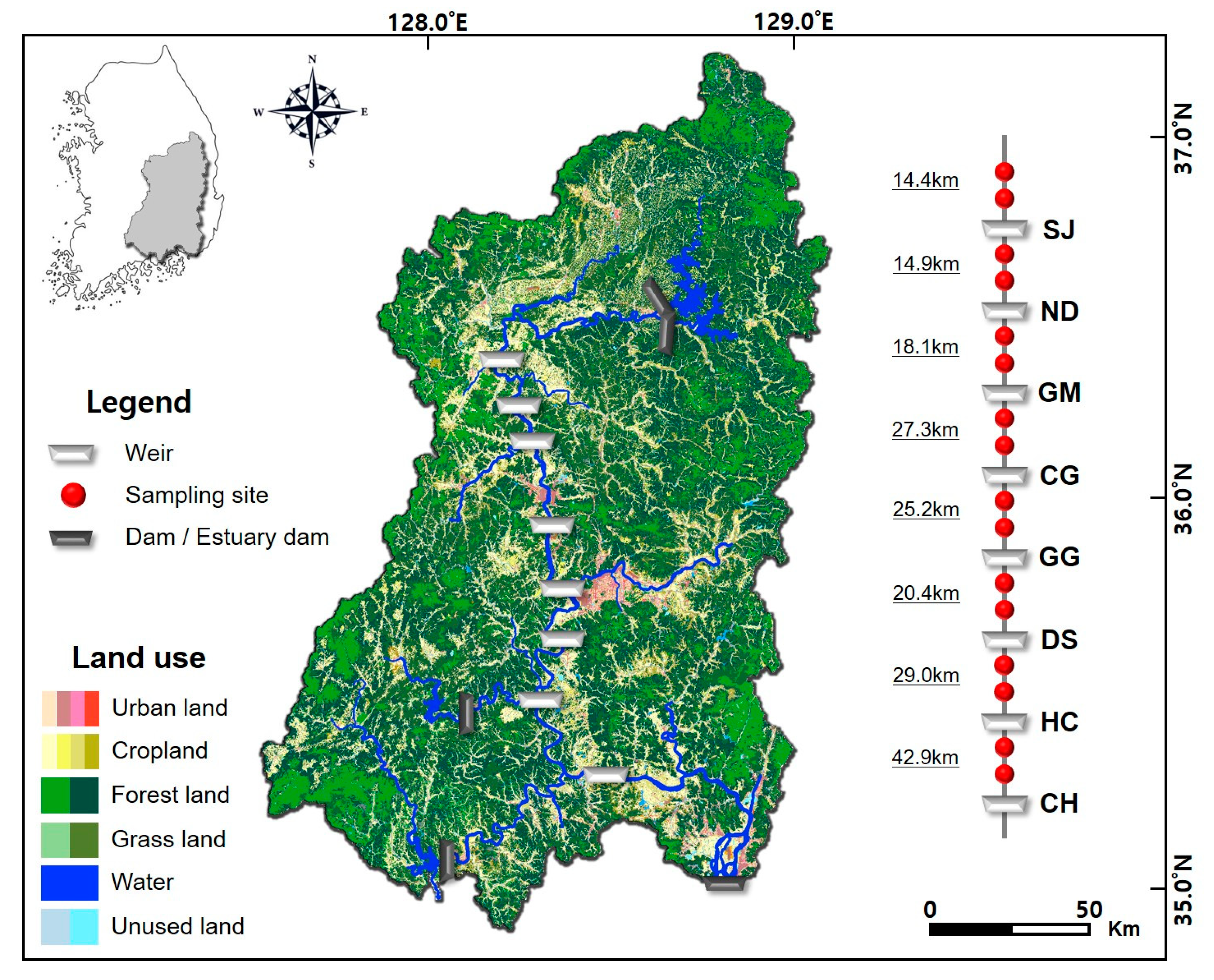
2.1. Study Area Description

The target of this study was the Nakdong River, located in the southeastern part of the Korean Peninsula (Nakdong River Basin, 34.6°–37.1° N, 127.3°–129.1° E) (Figure 1). The Nakdong River is the longest in Korea and flows into the South Sea with a total length of 510.36 km (the second-largest basin area in Republic of Korea, 23,384 km2). As the basin contains several large cities with more than one million people, such as Daegu, Changwon, and Busan, water is supplied to more than 13 million people yearly. In addition, agricultural water is supplied to 5260 km2 of agricultural land. The average annual precipitation in the Nakdong River Basin over ten years (2010–2019) was 1253 mm. Because the basin has an Asian monsoon climate, 70% of the annual precipitation is concentrated from June to August. In land cover maps of the basin, forest areas comprised the highest proportion (67.2%), followed by agricultural (22.7%), urban (4.5%), water and wetlands (2.8%), and other areas, including grasslands and bare lands (2.8%). The Korean government implemented the ‘Four Major Rivers Restoration Project’ from 2009 to 2012. The project aimed at flood control, water security and drought response, water quality improvement, ecological restoration, and waterfront development. Sixteen weirs were installed in four large rivers in Republic of Korea [8]. In the Nakdong River, the following eight weirs were installed in an approximately 207.3 km section (Table S1). The flow of the mainstream of the Nakdong River is controlled by large dams with an annual water supply of more than five million m3 and the Nakdong River Estuary Dam. The Nakdong River is a representative case of a natural river flow controlled by humans in all sections (Figure 1).

2.2. Data Collection Design

This study selected 16 survey points in the Nakdong River, where eight weirs were installed (Figure 1). Field surveys were conducted over 12 years from 2010 to 2021. Ecological surveys and environmental stressor surveys were conducted separately. Among the ecological surveys, fish surveys were conducted twice yearly before and after the monsoon rainfall period. The first survey was conducted in May–June, and the second one in September–October. Benthic macroinvertebrates surveys were conducted thrice yearly, before, during, and after monsoon rainfall. The first survey was conducted in April–May, the second in June–August, and the third in September–October. The survey date was selected during the survey period in consideration of weather conditions (e.g., precipitation) annually. Ecological surveys were conducted sequentially from upstream to downstream, and it took an average of 7 days after the start of the first sampling site. The environmental stress survey period was investigated weekly for 8 weeks before the ecological survey date, since it was considered that benthic macroinvertebrates require an average eight weeks exposure period for colonization [30].
For ecological surveys, selecting microhabitats that represent the diversity and representativeness of the biological assemblages within a designated survey scope is important. Ecological surveys were conducted with reference to the National Institute of Environmental Research of Korea [31]. Identification was mostly performed at the species level based on morphological characteristics of fish and macroinvertebrate. For the environmental data, 29 individual variables describing water quality conditions and 18 individual variables describing the habitat environment were acquired at the sampling site scale. A total of 19 individual variables representing hydrological characteristics were defined at the basin scale (Table 1). Some environmental stressors survey used the results of the monitoring by the Korean Ministry of Environment [32,33]. Further, the detailed descriptions of data collection designs are presented in Text S1.

2.3. Data-Driven Model Quantifying Biological Assembalge Response to Stressors

This study’s diagnostic tools for biodiversity responses were based on the GF model. The conceptual flow (framework) of the diagnostic tools used in this study is shown in Figure 2. The GF model was extended from the RF algorithm and is a new technique that directly constructs a function representing the compositional turnover of each biological assemblage according to environmental stressors [36]. In addition, interactions between species (or populations) can be reflected at the community level because the ‘assemble-and-predict-together’ approach defined by Ferrier and Guisan (2006) [37] was applied [38]. A GF model was constructed for each fish and benthic macroinvertebrate community. To meet statistical requirements, taxa relative abundances were log transformed. The benthic macroinvertebrate community targeted taxa with a relative abundance of 5% at each sampling site; however, the fish community included all taxa. Environmental stressors were not log transformed as this is a predictor variable in the GF models. Finally, the following four models were constructed: the fish response model during the weir construction period (2010–2012) (Fish.con), the fish response model during the weir operation period (2013–2021) (Fish.ope), the benthic macroinvertebrate response model during the weir construction period (Mac.con), and the benthic macroinvertebrate response model during the weir operation period (Mac.ope). A field dataset of all the biological response models (GF) was generated with a sample size of n = 867.
The GF models used the R packages, extended-Forest and gradient-Forest (version 3.5.3) [39]. The RF model, composed of 1000 regression trees for each species, was implemented using the extended-Forest package. Each regression tree was optimized according to the bootstrap sampling technique of the observed values. For data partitioning, the best split (error variance minimization) was performed by testing random subgroups of predictors (environmental stressors) [21,36]. The GF model provides three measurements to identify biodiversity responses: the goodness-of-fit measure Rf2 for species f, the accuracy importance Ifs for stressor s within the forest (species) f, and the raw importance Ifstv for that stressor at a split value v in a particular tree t. Rf2 is the variance ratio described by RF and is used as a measure that a particular species f is described by the overall stressors. Ifs indicates the importance of each stressor for a particular species f, and a zero or relatively low value indicates that the stressor has almost no predictive power.
The gradient-Forest package utilized all environmental stressors and biological assemblage information with an R2 of zero or higher in the extended-Forest package. The species compositional turnover functions for the environmental stressors were obtained by distributing the R2 values from all species among the stressors in proportion to their accuracy importance and along the stressor gradient according to the density of the raw importance [36]. The threshold for compositional turnover was defined based on the stressor values in the sections where the ratio between the raw split importance (black line in graph ④ in Figure 2) and the density function of the stressor (red line in graph ④ in Figure 2) exceeded 1 (Figure 2). Finally, specific-taxon cumulative importance plots were derived by accumulating the split importance according to environmental stressor gradients. The cumulative importance plots did not provide species response directionality according to environmental stressors; thus, the Pearson correlation coefficient between biological assemblages and environmental variables was analyzed. The management or ecological threshold of an individual species or a specific taxon was identified using a breakpoint and a section with a sharp change in the graph [20].
Ordination and vector fitting analyses were conducted to evaluate the relationship between the environmental stressors selected in the GF model and river biological assemblages. Ordination represented the abundance of each biological assemblage in the bubbles along two axes. In ordination, closer bubbles represent more similar biological sets, whereas distant bubbles represent sets with relatively different biological characteristics. Non-metric multidimensional scaling (NMDS) based on Bray–Curtis dissimilarities was generated for each biological group using the relative abundance data of the taxonomic groups selected in the GF model. In addition, the environmental variables selected in the GF model were overlapped with the ordination vector of each biological group using vector fitting analysis, and the ‘envfits’ function was used. The vector shows the direction and size of the environmental stressors related to the bubbles in the ordination. Vector analysis was statistically evaluated using an ordination-based test [40]. R statistical software (version 4.1.3) [39] was used for ordination and vector-fitting analyses.

3. Results

Field surveys identified a total of 51 fish species belonging to five orders, and 229 benthic macroinvertebrates species belonging to 27 orders (Table S2). Unlike the fish, benthic macroinvertebrates were only targeted to 121 species, excluding rare taxa (relative abundance of 5% at each survey point) in the GF model. One species of fish (Culter brevicauda (n = 32); F034; Tolerant species) and two species of benthic macroinvertebrates (Cristaria plicata (n = 1); B023) and Macromia daimoji (n = 22) (B052)) corresponded to legally protected species (endangered species). However, C. plicata (B023) did not meet the statistical requirement (relative abundance of 5% at each survey point), so it was not included in the GF model.

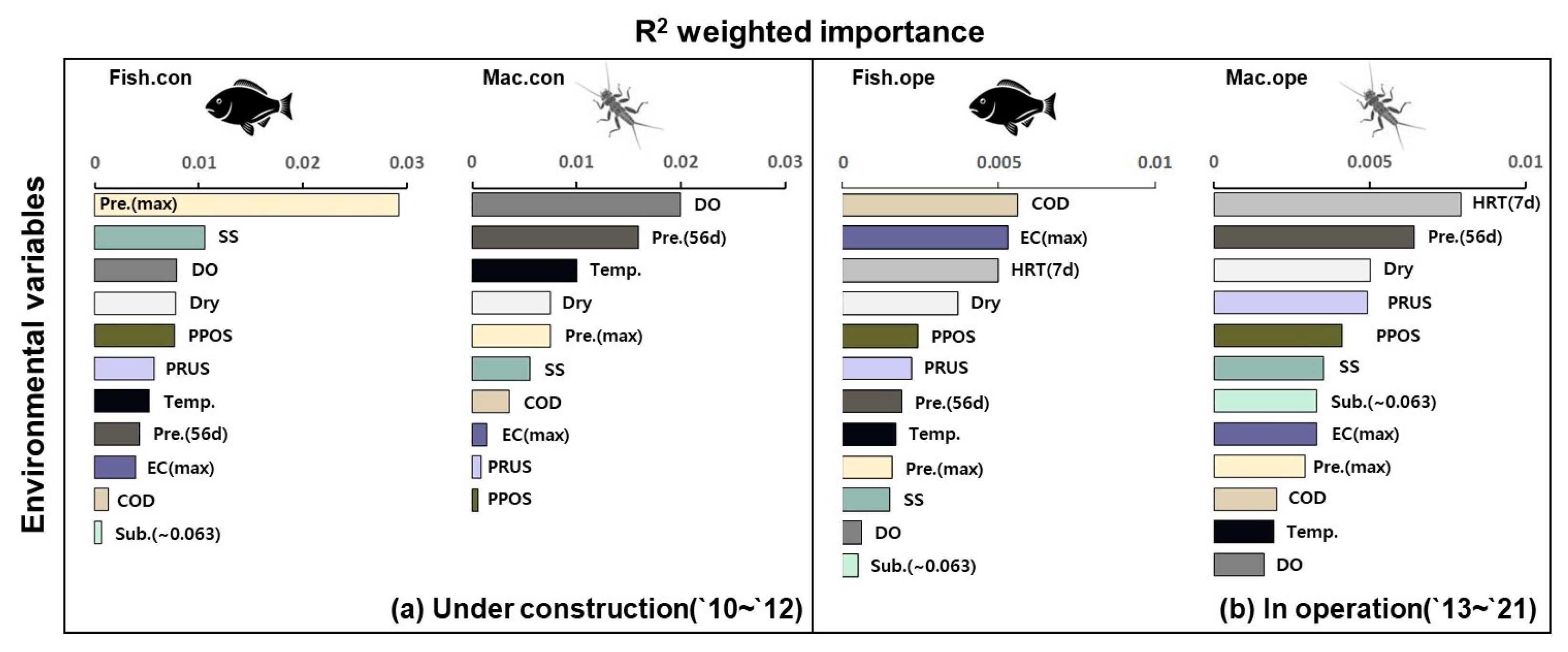
3.1. Overall Important Predictor of Biological Assemblage

The four response models were divided according to the weir construction period (2010–2012) and weir operation period (2013–2021) (Fish.con; Fish.ope; Mac.con; Mac.ope), and the most important environmental stressors explaining the distribution of fish and benthic macroinvertebrate communities were selected (Figure 3; Text S2). Split-density plots show sections where changes in the composition of biological assemblages occurred according to the gradients of the environmental predictive variables. As the ratio of split and data density, referred to as the compositional turnover rate, is higher than 1, relatively large community composition changes occur in the corresponding stressor concentration section [36]. In this study, sections with ratios >1 were identified, and the thresholds for environmental stressors that determined the distribution of fish and benthic invertebrate communities during the weir construction and operation periods are presented in Figure 4.
Consequently, the major environmental factors selected in the four biodiversity response models differed according to the biological assemblage. Precipitation and dissolved oxygen were the most important predictors in both fish and macroinvertebrate during construction of weirs. Whereas, during operation of weirs, chemical oxygen demand, hydraulic retention time and maximum conductivity were the most important predictors in both biological assemblage model. In addition, even within the same biological assemblage, the environmental stressors that determined community composition differed depending on the presence of weirs (Figure 3).

3.2. Specific-Taxon Response to Environmental Thresholds

Split-density plots provided points at which the composition of the biological assemblages changed as thresholds (Figure 4). In contrast, cumulative importance plots identified the thresholds for individual species (Figure 5). The four biodiversity response models constructed in this study identified similar points in the split density and cumulative importance plots as thresholds.
Cumulative importance plots of specific-taxon responses represent the top six taxa with the highest explanatory power for changes in environmental stressors. However, the selected taxa may vary depending on the environmental variables. In addition, they do not provide directionality to individual species. Here, ‘directionality for individual species’ means an increase or decrease in a particular species according to the environmental gradient direction. Therefore, in this study, individual species that met the statistical criteria (overall weighted importance R2 values were 0.015 or higher, and the R2 values of individual environmental stressors were 0.005 or higher) or were ecologically valuable (endangered species) among the taxa selected by the GF model (Figure S1) were selected as ‘major taxa’. In addition, the correlations between biological assemblages and environmental stressors were analyzed, and the directionality of species responses according to the environmental gradient is presented in Figure 5 (Tables S3 and S4). This novel approach adjusts for the number of unnecessary relationships between biological assemblages and environmental variables, such that statistically explainable taxa and environmental stressors can be identified. Ultimately, this enables a more powerful and easy interpretation of the responses of individual species to multiple variables [10].

3.2.1. Fish

Among the fish response models that used 51 species, 12 species in the weir construction model (Fish.con) and 20 species in the weir operation model (Fish.ope) were selected as taxa that could be explained by environmental stressors (Figure S1). Legally protected species (Culter brevicauda (n = 32); F034; Tolerant species), including endangered species, were not selected in the GF model.
The fish response model for the weir construction period selected Tridentiger bifasciatus (F030; Intermediate species), Rhinogobius brunneus (F031; Intermediate species), Micropterus salmoides (F033; Tolerant species), Acanthorhodeus macropterus (F050; Intermediate species), and Zacco platypus (F051; Intermediate species) as the ‘major taxa’ (Table S3). Rhinogobius brunneus (F031; Intermediate species) and Tridentiger bifasciatus (F030; Intermediate species), which are riffle-benthic species [1], exhibited positive responses to maximum daily precipitation (Pre. (max)), and the threshold was 80 mm. In contrast, Micropterus salmoides (F033; Tolerant species) showed a negative response, and the threshold was lower (60 mm) (Figure 5a). Zacco platypus (F051; Intermediate species) showed a negative relationship with SS at a threshold of 20 mg/L (Figure 5b). Meanwhile, for Carassius auratus (F037; Intermediate species), which is not included in the ‘major taxa’ but has high weighted importance, the community composition ratio was determined by the characteristics of the habitat environment (Figure S1). Carassius auratus (F037; Intermediate species) exhibited a threshold response when the proportion of runs within the sampling site (PRUS) was 15% or lower, the proportion of pools (PPOS) was 85% or higher, and the number of dry days (Dry) was 28 or higher (Figure S2).
During the weir operation period, Opsariichthys uncirostris amurensis (F011; Tolerant species), Tridentiger bifasciatus (F030; Intermediate species), Micropterus salmoides (F033; Tolerant species), Carassius auratus (F037; Intermediate species), and Lepomis macrochirus (F038; Tolerant species) were selected as ‘major taxa’ (Table S4). Micropterus salmoides (F033; Tolerant species) and Lepomis macrochirus (F038; Tolerant species), which are non-native species, responded positively to COD and EC (max). A gradual response was observed for COD at a 4 mg/L threshold. For EC (max), the response rapidly increased from a threshold of 210 ㎲/㎝ (Figure 5c,d). Acheilognathus yamatsutae (F043; Intermediate species), a Korean endemic species, showed an opposite response (negative relationship) to COD and EC (max) compared to non-native species. In particular, it exhibited management thresholds that require immediate management at 4.6 mg/L (COD) and 250 ㎲/㎝ (EC (max)) (Figure 5c,d). Meanwhile, Micropterus salmoides (F033; Tolerant species) and Lepomis macrochirus (F038; Tolerant species), which are non-native species, and Tridentiger bifasciatus (F030; Intermediate species), a riffle-benthic species, showed a positive relationship with the weekly average hydraulic retention time (HRT (7d)) (Figure 5e).

3.2.2. Macroinvertebrate

Among the benthic macroinvertebrate response models that used 121 species, 14 species in the weir construction model (Mac.con) and 18 species in the weir operation model (Mac.ope) were selected as taxa that could be explained by environmental stressors (Figure S1). Among these, one endangered species (Macromia daimoji (B052)) was included in the weir operation model.
During the weir construction period, Chironomidae (non-red type) (B030), Micronecta (Basileonecta) sedula (B040), Simulium sp. (B089), Siphlonurus chankae (B172), and Macrobrachium nipponese (B208) were selected as ‘major taxa’ (Table S3). Chironomidae (non-red type) (B030) and Micronecta (Basileonecta) sedula (B040) were positively correlated with DO (Figure 5f). In contrast, the 56-day cumulative precipitation (Pre. (56d)) had a negative relationship with Micronecta (Basileonecta) sedula (B040) and Macrobrachium nipponese (B208) (Figure 5g). Micronecta (Basileonecta) sedula (B040) and Siphlonurus chankae (B172) showed negative responses to water temperature (Temp.); however, their thresholds differed (Figure 5h). Consequently, in the weir construction model, the relative abundance of Micronecta (Basileonecta) sedula (B040) increased in the water body where the water temperature (Temp.) of 20 °C or less, a DO value of 13 mg/L or higher, and 56-day cumulative precipitation (Pre. (56d)) of 250 mm or less was maintained. These GF model results were confirmed by the relative abundance of Micronecta (Basileonecta) sedula (B040) during weir operation. Among the ‘major taxa’ selected in the Mac.con model, Simulium sp. (B089) and Siphlonurus chankae (B172) had apparent thresholds for environmental stressors (DO; Pre. (56d), and Temp.). For example, management thresholds of Siphlonurus chankae (B172) were identified as 130 mm for a 56-day cumulative precipitation (Pre. (56d)) (Figure 5g). However, the number of field samples used was insufficient (Figure S7).
During the weir operation period, Procloeon pennulatum (B007), Chironomidae (red-type) (B031), Micronecta (Basileonecta) sahlbergii (B068), Ephydridae (B097), Limnodrilus gotoi (B143), and Pectinatella magnifica (statoblasts) (B218) were selected as the ‘major taxa’ (Table S4). Limnodrilus gotoi (B143) showed a gradual negative response to the weekly average hydraulic retention time (HRT (7d)) (no clear threshold); however, Micronecta (Basileonecta) sahlbergii (B068) and Ephydridae (B097), which are arthropods (insects), were found to have a positive correlation. However, the thresholds for the two arthropod species were different (0 and 16 d) (Figure 5i). Pectinatella magnifica (statoblasts) (B218) showed a positive response to 56-day cumulative precipitation (Pre. (56d)), and the threshold was 360 mm (Figure 5j). It exhibited a negative response to the number of dry days (DRY), and the threshold was identified on days 15 and 25 (Figure 5k). In the weir operation model, the composition distribution of Macromia daimoji (B052) was explained by the COD and EC (max) in the ‘water quality’ category. For example, 5.3 mg/L (COD) and 220 µs/cm (EC(max)) were identified as management thresholds that require immediate management (Figure S3). However, the number of field samples used was insufficient (Figure S4).

3.3. Comparison of Two Methods (The GF Models and the NMDS Plot)

To explain the relationship between the major taxa selected in the GF model and the environmental stressors, a non-metric multidimensional scaling ordination plot was constructed. NMDS analysis expressed the final selected environmental stressors in the ordination plot and GF model, which indicated the relative abundances of major taxa as vectors.
The NMDS ordination plots of the fish and benthic macroinvertebrate taxa generally agreed with the biological responses to the major environmental stressors selected in the GF model (Figure 6; Tables S3 and S4). For example, during the weir construction period, Tridentiger bifasciatus (F030; Intermediate species) and Zacco platypus (F051; Intermediate species) exhibited higher relative abundances at sampling sites with high Pre.max and low abundances at sampling sites with high SS (Figure 6b,c). During the weir operation period, Micropterus salmoides (F033; Tolerant species) and Lepomis macrochirus (F038; Tolerant species) showed higher relative abundances at sampling sites with high COD and EC (max) concentrations and a long HRT (7d) (Figure 6d–f). During the weir construction period, Chironomidae (non-red type) (B030) and Micronecta (Basileonecta) sedula (B040) showed lower relative abundances at sampling sites with high Temp. and Pre. and a higher relative abundance at sampling sites with high DO (Figure 6g–i). Chironomidae (red type) (B031) and Pectinatella magnifica (statoblasts) (B218) showed conflicting characteristics during the weir operation (Figure 6j–l). These characteristics were also confirmed by the relative abundance distribution chart of the two species (Figure S8).

4. Discussion

4.1. Specific-Taxon Response to Multi-Stressors

To distinguish the environmental stressors that changed the biological assemblage composition in a large river, four biodiversity response models were constructed using biological assemblages (fish or benthic macroinvertebrates) and conditions (weir construction or operation). Environmental stressors that determine the biological assemblage composition in the large river with weirs were different depending on the ‘conditions of weir construction and operation’ and ‘fish and benthic macroinvertebrates’ (Figure 3). These discrepancies (environmental stressors) between models can be attributed to differences in the ‘major taxa’ selected in the GF model (Figure S1) [36]. The GF model is a statistical technique that selects specific species with distinct changes in the composition ratio within a biological assemblage according to the environmental gradient (‘major taxa’) (Figure S1) and quantitatively analyzes their relationships with environmental stressors [36]. Species whose relative abundance did not change within the biological assemblage according to their environmental gradient (for example, even if they were dominant in all samples) were not selected as major taxa in the GF model [20]. Therefore, the results of this study can explain how multiple environmental stressors that occurred during the weir construction and operation periods affected changes in ‘major taxa.’
For example, the composition ratios of Micropterus salmoides (F033; Tolerant species) and Lepomis macrochirus (F038; Tolerant species) increased under habitat conditions of maximum daily precipitation (Pre. (max)) of 60 mm or less, a COD value of 5 mg/L or higher, an EC (max) value of 210 µs/cm or higher, and a weekly average hydraulic retention time (HRT (7d)) value of 20 days or more (Figure 5a,c–e). In the benthic macroinvertebrate response model (Mac.ope), Chironomidae (red type) (B031) and Limnodrilus gotoi (B143) are legal pollution indicator species designated by the Korean government [41]. Their relative abundance was found to increase when the weekly average hydraulic retention time (HRT (7d)) was 20 days or more and the number of dry days (Dry) was 30 days or more (Figure 5j,k). These four taxa were selected as ‘major taxa’ with high weighted importance R2 in the weir operation models (Fish.ope and Mac.ope), indicating that their importance increased due to changes in environmental stressors (F033 and F038 in Figure S6; B031 and B143 in Figure S8). Actually, the ecological information (e.g., preference of water bodies with high organic pollution and slow flow) of legal pollution indicator (B031, B043) species and non-native species (F033, F038) were similar to that previously reported in Korean freshwater [42,43,44]. Consequently, many studies have verified an increase in the aforementioned four species of large river sections [1,8,43,45]. Therefore, this study demonstrates that identifying the environmental stressors that distinguish large-scale physical disturbances, such as weir construction and operation, by applying diagnostic tools that use multiple biological assemblages is necessary. Third, the selection of environmental stressors using statistical techniques is a considerable methodology, which can improve the limitation of reflecting environmental stressors with the same weight for all taxa [46,47].

4.2. Effors to Identify ‘True’ Thresholds

In a study based on field data, careful interpretation is required because the identification of thresholds relies solely on analytical techniques (GF and TITAN) [20,48]. In this study, the problems encountered during the identification of ‘true’ thresholds using the GF model were summarized. First, thresholds with unrealistically high values were identified in some models (Fish.con and Mac.ope) (Figure 4a,b,j). These thresholds might be related to outliers with extremely high environmental stressor concentrations [27]. This finding contradicts that of a previous study that reported that the GF model based on regression tree techniques is robust against outliers [49]. Second, certain species that did not have sufficient n values in the field data were selected as ‘major taxa’ in some models (B089 and B172 in Figure S7; B068 and B218 in Figure S8). The detection of ‘major taxa’ with insufficient field data (n < 10) can be caused by unrealistic statistical assumptions; such as when interpreting thresholds from uniform distributed data according to the environmental gradient (e.g., datasets with skewed environmental distribution, but with uniform species responses) [20,48]. This was due to the distribution and shape of the biological assemblages according to the environmental gradient directly affecting the model performance [50]. Sultana et al. (2020) [20] mentioned that the GF model has an excellent ability to detect the thresholds of “multiple abrupt change points”, which can be proven by sufficiently secured large amounts of data. They also advised that a sufficient examination (prior screening of data structures and interpretation through ecological information) is required to interpret the threshold derived from low data density.
To address the problems mentioned above, the GF model results were analyzed in parallel with the NMDS (Figure 6), field data (Figures S5–S8), and ecological information. Consequently, thresholds with unrealistically high values and the interpretation of ‘major taxa’ for which field data were insufficient (n < 10) or ‘directionality’ did not match field data were excluded from the results. Interpretations were performed using ecological information for species with high ecological value, such as endangered and Korean endemic species. Macromia daimoji, a legal protection species (endangered species), and Acheilognathus yamatsutae, a Korean endemic species, prefer water bodies with low organic contamination. In addition, unlike Pectinatella magnifica (adults), which appear in stagnant water bodies, such as pools, statoblasts are spread by heavy rainfall [51]. These characteristics are also in agreement with the results of Pectinatella magnifica (statoblasts) confirmed in this study.

4.3. Preservation Implicatrion Using Environmental Thresholds

Several studies have reported the effects of weir on biological assemblages in large rivers. These studies commonly identify environmental stressors that change biological assemblages using statistical techniques [1,2,3,52]. However, certain criteria are required to establish guidelines for the preservation of river ecosystems [53,54]. This requires efforts to identify taxon-specific thresholds [20]. Efforts have been made to apply thresholds to establish environmental management criteria in many environmentally advanced countries, such as the United States [10,27], Canada [55], Australia and New Zealand [20], Brazil [23], and Italy [54]. However, studies on this topic in Korea are limited [52].
Due to the lack of sufficient biological information and studies on thresholds during the weir operation period [11], it cannot be guaranteed that the management thresholds confirmed in this study are irreversible values that indicate the elimination of the species [56]. The fact that exceeding thresholds significantly reduces the diversity and resilience of biological assemblages, however, was proven through many studies [10,23,27]. In this study, the thresholds of non-native species (Micropterus salmoides, Lepomis macrochirus), a Korean endemic species (Acheilognathus yamatsutae), an endangered species (Macromia daimoji), and legal pollution indicator species (Chironomidae (red type), Limnodrilus gotoi) were presented using fish- and benthic macroinvertebrate-based diagnostic tools.
These diagnostic tools can be used to identify environmental stressors that must be managed first and their reference points for the preservation of endangered species and control of non-native species. If more investigations and studies are conducted over the long term, management thresholds for decision-making are expected to be used as environmental stressor guidelines for the preservation of endangered species and management of non-native species [23,26,55]. This may ultimately enable a sustainable aquatic ecosystems maintenance and biodiversity preservation.

5. Conclusions

A threshold analysis method that utilizes multiple biological assemblages is a useful diagnostic tool that enables the identification of the ranges (levels) of environmental stressors that can replace or eliminate certain species by quantifying the nonlinear relationships between changes in environmental stressors and biodiversity. Based on this, presenting tangible management goals for the preservation of river biodiversity (guidelines for the preservation of endangered species) is possible. This study identified the major environmental stressors of community turnover and corresponding thresholds by applying diagnostic tools that use multiple biological assemblages in a large river with artificially controlled flow. The following conclusions were drawn:
i.
The community turnover and thresholds that responded multi-stressors differed depending on the biological assemblage, even under the same environmental conditions. In particular, operation weirs have increased the importance of certain species (e.g., non-native species). Therefore, it was confirmed that diagnostic tools that use multiple biological assemblages can be useful for identifying multiple environmental stressors caused by large artificial structures such as weirs.
ii.
Thresholds for each type of major taxon were identified in a large river with weirs, which are the first reference points presented in similar ecological environments. In the long term, this approach can be used as a guideline for major taxa that must be managed from a biodiversity perspective.
iii.
The limitations of the Gradient Forest (GF) technique (machine learning method), which is dependent on field data due to its characteristics, were found while identifying ‘true’ thresholds. Therefore, reliable results were obtained by applying several processes (comparison with field data, interpretation through ecological information, and application of similar statistical techniques).
Understanding these thresholds and their roles is important for biodiversity preservation to manage the multiple environmental stressors that occur in ecosystems. Unfortunately, research on the thresholds to support ecosystem management has only recently begun in South Korea. Therefore, sufficient research needs to be conducted on various river ecosystems with weirs and taxa within the scope of similar analytical frameworks.

Supplementary Materials

The following supporting information can be downloaded at: https://www.mdpi.com/article/10.3390/su16177447/s1, Figure S1: The goodness of fit of the important taxa was calculated using the four biological assemblage response models of the Gradient Forest. The red dotted lines and boxes denote the ‘major taxa’ with high explanatory power (R2 values above 0.15). For taxon codes (B040), see Supplementary Materials, Table S3; Figure S2: Cumulative importance plots for Carassius auratus (F037; Tolerant species) along the PRUS, PPOS, and Dry gradients calculated from the fish response model (Fish.con). The blue lines indicate the threshold corresponding to significant changes in the taxa response. “+” and “−” in the bracket signify positive and negative relationships, respectively, for the species to the variable; Figure S3: Cumulative importance plots of the endangered taxon (Macromia daimoji; B052) along the EC (max) and COD gradient calculated from the macroinvertebrate response model (Mac.ope). Green lines indicate the threshold corresponding to the significant change in taxa response. “+” and “-” signify positive and negative relationships, respectively, for the species to the variable; Figure S4: Relative abundance changes (b,d) of Macromia daimoji (B052) along an increasing (a) EC (max) and (c) COD gradient during the ‘in operation’ identified by the macroinvertebrate assemblage response model of the Gradient Forest; Figure S5: Relative abundance changes of the five most important taxa with increasing (a) pre. (max) and (b) suspended solid (SS) gradient during ‘under construction’ as identified by the fish assemblage response model of the Gradient Forest; Figure S6: Relative abundance changes of the five most important taxa along increasing (a) COD, (b) EC (max), and (c) HRT (7d) gradient during the ‘in operation’ identified by the fish assemblage response model of the Gradient Forest; Figure S7: Relative abundance changes of the five most important taxa with increasing (a) dissolved oxygen (DO), (b) Pre. (56d), (c) Water temperature (Temp.) gradient during ‘under construction’ identified by the macroinvertebrate assemblage response model of the Gradient Forest; Figure S8: Relative abundance changes of the five most important taxa with increasing (a) HRT (7d), (b) Pre. (56d), and (c) dry day (Dry) gradient during the ‘under construction’ identified by the macroinvertebrate assemblage response model of the Gradient Forest; Table S1: Hydrological and morphological information for eight weirs installed in the Nakdong River, Republic of Korea; Table S2: Taxon codes corresponding to species names used in the Gradient Forest Model; Table S3: List of each biological assemblage with R2 values equal or above 0.15 for Gradient Forest models (* R2 ≥ 0.20, ** R2 ≥ 0.30) and associated environmental parameter by stressors (listed variables have individuals R2 ≥ 0.02) under construction of weir. “+” and “-” signify positive and negative relationships, respectively, for the species to the variable; Table S4: List of each biological assemblage with R2 values equal or above 0.15 for Gradient Forest models (* R2 ≥ 0.20, ** R2 ≥ 0.30) and associated environmental parameter by stressors (listed variables have individuals R2 ≥ 0.02) in the weir operation. “+” and “−” signify positive and negative relationships, respectively, for the species to the variable. For variable definitions and units, see Supplementary Materials, Table S1.

Author Contributions

Conceptualization, H.-S.R.; validation, H.-K.P.; formal analysis, J.H.; investigation, J.H. and K.-J.P.; data curation, K.-J.P.; writing—original draft preparation, H.-S.R.; writing—review and editing, J.H. and H.-K.P.; visualization, J.H.; supervision, H.-K.P.; project administration, H.-S.R. All authors have read and agreed to the published version of the manuscript.

Funding

This work was supported by a grant from the National Institute of Environmental Research (NIER), funded by the Ministry of Environment (ME) of the Republic of Korea (NIER-2022-04-02-083).

Institutional Review Board Statement

Not applicable.

Informed Consent Statement

Not applicable.

Data Availability Statement

The data presented in this study are available on request from the corresponding author.

Conflicts of Interest

The authors declare no conflicts of interest.

References

  1. Atique, U.; Kwon, S.; An, K. Linking weir imprints with riverine water chemistry, microhabitat alterations, fish assemblages, chlorophyll-nutrient dynamics, and ecological health assessments. Ecol. Indic. 2020, 117, 106652. [Google Scholar] [CrossRef]
  2. Tóth, R.; Czeglédi, I.; Kern, B.; Erős, T. Land use effects in riverscapes: Diversity and environmental drivers of stream fish communities in protected, agricultural and urban landscapes. Ecol. Ind. 2019, 101, 742–748. [Google Scholar] [CrossRef]
  3. Miao, Y.; Li, J.; Feng, P.; Dong, L.; Zhang, T.; Wu, J.; Katwal, R. Effects of land use changes on the ecological operation of the Panjiakou-Daheiting Reservoir system, China. Ecol. Eng. 2020, 152, 105851. [Google Scholar] [CrossRef]
  4. Salant, N.L.; Schmidt, J.C.; Budy, P.; Wilcock, P.R. Unintended consequences of restoration: Loss of riffles and gravel substrates following weir installation. J. Environ. Manag. 2012, 109, 154–163. [Google Scholar] [CrossRef] [PubMed]
  5. Merg, M.L.; Dézerald, O.; Kreutzenberger, K.; Demski, S.; Reyjol, Y.; Usseglio-Polatera, P.; Belliard, J. Modeling diadromous fish loss from historical data: Identification of anthropogenic drivers and testing of mitigation scenarios. PLoS ONE 2020, 15, e0236575. [Google Scholar] [CrossRef]
  6. Petts, G.E.; Gurnell, A.M. Dams and geomorphology: Research progress and future directions. Geomorphology 2005, 71, 27–47. [Google Scholar] [CrossRef]
  7. Maceda-Veiga, A.; Mac Nally, R.; de Sostoa, A. The presence of non-native species is not associated with native fish sensitivity to water pollution in greatly hydrologically altered rivers. Sci. Total Environ. 2017, 607–608, 549–557. [Google Scholar] [CrossRef]
  8. Jo, H.; Jeppesen, E.; Ventura, M.; Buchaca, T.; Gim, J.S.; Yoon, J.D.; Kim, D.H.; Joo, G.J. Responses of fish assemblage structure to large-scale weir construction in riverine ecosystems. Sci. Total Environ. 2019, 657, 1334–1342. [Google Scholar] [CrossRef] [PubMed]
  9. van Oorschot, M.; Kleinhans, M.; Buijse, T.; Geerling, G.; Middelkoop, H. Combined effects of climate change and dam construction on riverine ecosystems. Ecol. Eng. 2018, 120, 329–344. [Google Scholar] [CrossRef]
  10. Waite, I.R.; Pan, Y.; Edwards, P.M. Assessment of multi-stressors on compositional turnover of diatom, invertebrate and fish assemblages along an urban gradient in Pacific Northwest streams (USA). Ecol. Indic. 2020, 112, 106047. [Google Scholar] [CrossRef]
  11. Haase, P.; Pilotto, F.; Li, F.; Sundermann, A.; Lorenz, A.W.; Tonkin, J.D.; Stoll, S. Moderate warming over the past 25 years has already reorganized stream invertebrate communities. Sci. Total Environ. 2019, 658, 1531–1538. [Google Scholar] [CrossRef]
  12. Alric, B.; Dézerald, O.; Meyer, A.; Billoir, E.; Coulaud, R.; Larras, F.; Mondy, C.P.; Usseglio-Polatera, P. How diatom-, invertebrate- and fish-based diagnostic tools can support the ecological assessment of rivers in a multi-pressure context: Temporal trends over the past two decades in France. Sci. Total Environ. 2021, 762, 143915. [Google Scholar] [CrossRef] [PubMed]
  13. Ozolinš, D.; Skuja, A.; Jēkabsone, J.; Kokorite, I.; Avotins, A.; Poikane, S. How to assess the ecological status of highly humic lakes? Development of now method based on benthic invertebrates. Water 2021, 13, 223. [Google Scholar] [CrossRef]
  14. Poikane, S.; Várbíró, G.; Kelly, M.G.; Birk, S.; Phillips, G. Estimating river nutrient concentration consistent with good ecological condition: More stringent nutrient thresholds needed. Ecol. Ind. 2021, 121, 107017. [Google Scholar] [CrossRef]
  15. Vitecek, S.; Johnson, R.K.; Poikane, S. Assessing the ecological status of European rivers and lakes using benthic invertebrate communities: A practical catalogue of metrics and methods. Water 2021, 13, 346. [Google Scholar] [CrossRef]
  16. Kelly, M.G.; Whitton, B.A. The trophic diatom index: A new index for monitoring eutrophication in rivers. J. Appl. Phycol. 1995, 7, 433–444. [Google Scholar] [CrossRef]
  17. Mondy, C.P.; Usseglio-Polatera, P. Using conditional tree forests and life history traits to assess specific risks of stream degradation under multiple pressure scenario. Sci. Total Environ. 2013, 461 462, 750–760. [Google Scholar] [CrossRef]
  18. Larras, F.; Billoir, E.; Gautreau, E.; Coulaud, R.; Rosebery, J.; Usseglio-Polatera, P. Assessing anthropogenic pressures on streams: A random forest approach based on benthic diatom communities. Sci. Total Environ. 2017, 586, 1101–1112. [Google Scholar] [CrossRef]
  19. Dézerald, O.; Mondy, C.P.; Dembski, S.; Kreutzenberger, K.; Reyjol, Y.; Chandesris, A.; Valette, L.; Brosse, S.; Toussaint, A.; Belliard, J.; et al. A diagnosis-based approach to assess specific risks of river degradation in a multiple pressure context: Insights from fish communities. Sci. Total Environ. 2020, 734, 139467. [Google Scholar] [CrossRef]
  20. Sultana, J.; Tibby, J.; Recknagel, F.; Maxwell, S.; Goonan, P. Comparison of two commonly used methods for identifying water quality thresholds in freshwater ecosystems using field and synthetic data. Sci. Total Environ. 2020, 724, 137999. [Google Scholar] [CrossRef]
  21. Wagenhoff, A.; Clapcott, J.E.; Lau, K.E.M.; Lewis, G.D.; Young, R.G. Identifying congruence in stream assemblage thresholds in response to nutrient and sediment gradients for limit setting. Ecol. Appl. 2017, 27, 469–484. [Google Scholar] [CrossRef]
  22. Waite, I.R.; Munn, M.D.; Moran, P.W.; Konrad, C.P.; Nowell, L.H.; Meador, M.R.; Van Metre, P.C.; Carlisle, D.M. Effects of urban multi-stressors on three stream biotic assemblages. Sci. Total Environ. 2019, 660, 1472–1485. [Google Scholar] [CrossRef]
  23. Anunciação, P.R.; Barros, F.M.; Ribeiro, M.C.; Carvalho, L.M.; Ernst, R. Taxonomic and functional threshold responses of vertebrate communities in the Atlantic Forest Hotspot. Biol. Conserv. 2021, 257, 109137. [Google Scholar] [CrossRef]
  24. Moon, M.Y.; Ji, C.W.; Lee, D.-S.; Lee, D.-Y.; Hwang, S.-J.; Noh, S.-Y.; Kwak, I.-S.; Park, Y.-S. Characterizing responses of biological trait and functional diversity of benthic macroinvertebrates to environmental variables to develop aquatic ecosystem health assessment index. Korean J. Ecol. Environ. 2020, 53, 31–45. [Google Scholar] [CrossRef]
  25. Schinegger, R.; Palt, M.; Segurado, P.; Schmutz, S. Untangling the effects of multiple human stressors and their impacts on fish assemblages in European running waters. Sci. Total Environ. 2016, 573, 1079–1088. [Google Scholar] [CrossRef]
  26. Feng, C.; Li, H.; Yan, Z.; Wang, Y.; Wang, C.; Fu, Z.; Liao, W.; Giesy, J.P.; Bai, Y. Technical study on national mandatory guideline for deriving water quality criteria for the protection of freshwater aquatic organisms in China. J. Environ. Manag. 2019, 250, 109539. [Google Scholar] [CrossRef]
  27. Nichols, J.D.; Eaton, M.J.; Martin, J. Thresholds for conservation and management: Structured decision making as a conceptual framework. In Application of Threshold Concepts in Natural Resource Decision Making; Guntenspergen, G., Ed.; Springer: New York, NY, USA, 2014; pp. 9–28. [Google Scholar]
  28. Baker, M.E.; King, R.S. A new method for detecting and interpreting biodiversity and ecological community thresholds. Methods Ecol. Evol. 2010, 1, 25–37. [Google Scholar] [CrossRef]
  29. Bennett, E.M.; Balvanera, P. The future of production systems in a globalized world. Front. Ecol. Environ. 2007, 5, 191–198. [Google Scholar] [CrossRef]
  30. Barbour, M.T.; Gerritsen, J.; Snyder, B.D. Rapid Bioassessment Protocols for Use in Streams and Wadeable Rivers: Periphyton, Benthic Macroinvertebrates and Fish, 2nd ed.; Environmental Protection Agency, Office of Water: Washington, DC, USA, 1999. [Google Scholar]
  31. NIER (National Institute of Environmental Research). Guidelines on Investigating the Current Status of Aquatic Ecosystems and Assessment Method of Integrity; The Ministry of Environment (ME): Incheon, Republic of Korea, 2019. [Google Scholar]
  32. WEIS (Water Environment Information System). Water Quality Monitoring System by Ministry of Environment. Available online: https://water.nier.go.kr/web (accessed on 15 May 2021).
  33. WIP (Water Information Portal). Real-Time Weir Operation Information by K-Water of the Republic of Korea: My Water Database. Available online: https://www.water.or.kr/kor/menu/sub.do?menuId=13_91_93 (accessed on 11 May 2021).
  34. Craig, D.A. Some of what you should know about water of K.I.S.S. for hydrodynamics (*Keeping It Stupidly Simple). Bull. North Am. Benthol. Soc. 1987, 4, 178–182. [Google Scholar]
  35. Cummins, K.W. An Evaluation of some techniques for the collection and analysis of benthic samples with special emphasis on lotic waters. Am. Midl. Nat. 1962, 67, 477–504. [Google Scholar] [CrossRef]
  36. Ellis, N.; Smith, S.J.; Pitcher, C.R. Gradient forests: Calculating importance gradients on physical predictors. Ecology 2012, 93, 156–168. [Google Scholar] [CrossRef]
  37. Ferrier, S.; Guisan, A. Spatial modelling of biodiversity at the community level. J. Appl. Ecol. 2006, 43, 393–404. [Google Scholar] [CrossRef]
  38. D’Amen, M.; Rahbek, C.; Zimmermann, N.E.; Guisan, A. Spatial predictions at the community level: From current approaches to future frameworks. Biol. Rev. Camb. Philos. Soc. 2017, 92, 169–187. [Google Scholar] [CrossRef]
  39. R Core Team. R: A Language and Environment for Statistical Computing; R Foundation for Statistical Computing: Vienna, Austria, 2017; Available online: https://www.R-project.org/ (accessed on 10 January 2023).
  40. Oksanen, J.; Blanchet, F.G.; Friendly, M.; Kindt, R.; Legendre, P.; McGlinn, D.; Minchin, P.R.; O’Hara, R.B.; Simpson, G.L.; Solymos, P.; et al. Multivariate Analysis of Ecological Communities in R: Vegan Tutorial. R Package. Version 2.5-3. 2018. Available online: https://www.researchgate.net/publication/275524120_Multivariate_analysis_of_ecological_communities_in_R_vegan_tutorial_R_package_version_17 (accessed on 10 January 2023).
  41. EFE (Enforcement Decree of the Framework act on Environmental policy) Ministry of Government Legislation, Korean Law Information Center. Available online: https://www.law.go.kr/LSW/eng/engLsSc.do?menuId=2&section=lawNm&query=%ED%99%98%EA%B2%BD%EC%A0%95%EC%B1%85&x=0&y=0#liBgcolor1/ (accessed on 10 January 2023).
  42. Kang, Y.-J.; Lee, S.-J.; An, K.-G. Physical habitat and chemical water quality characteristics on the distribution patterns of ecologically disturbing fish (Largemouth bass and Blugill) in Dongjin-River Watershed. Korean J. Environ. Biol. 2019, 37, 177–188. [Google Scholar] [CrossRef]
  43. Wang, J.H.; Park, H.J.; Park, J.H.; Song, H.S.; Kim, H.J.; Park, Y.J.; Choi, J.K.; Lee, H.G. Comparison of the habitat distribution characteristics of aquatic Oligochaeta according to the construction of weirs in four major rivers in South Korea. Korean J Environ. Biol. 2019, 37, 607–617. [Google Scholar] [CrossRef]
  44. Kim, W.; Park, J.; Hong, C.; Choi, B.; Kim, H.; Park, Y.; Park, J.; Song, H.; Kwak, I. Changes in Community Structure of Chironomidae Caused by Variability of Environmental Factor among Weir Sections in Korean Rivers. Korean J. Ecol. Environ. 2020, 53, 46–54. [Google Scholar] [CrossRef]
  45. Jung, S.W.; Kim, Y.-H.; Lee, J.-H.; Kim, D.-G.; Kim, M.-K.; Kim, H.-M. Biodiversity changes and community characteristics of benthic macroinvertebrates in weir section of the Nakdong River, South Korea. Korean J. Environ. Ecol. 2022, 36, 150–164. [Google Scholar] [CrossRef]
  46. Simionov, I.-A.; Călmuc, M.; Iticescu, C.; Călmuc, V.; Georgescu, P.-L.; Faggio, C.; Petrea, Ş.-M. Human health risk assessment of potentially toxic elements and microplastics accumulation in products from the Danube River Basin fish market. Environ. Toxicol. Pharmacol. 2023, 104, 104307. [Google Scholar] [CrossRef]
  47. Iticescu, C.; Georgescu, L.P.; Murariu, G.; Topa, C.; Timofti, M.; Pintilie, V.; Arseni, M. Lower Danube Water Quality Quantified through WQI and Multivariate Analysis. Water 2019, 11, 1305. [Google Scholar] [CrossRef]
  48. Daily, J.P.; Hitt, N.P.; Smith, D.R.; Snyder, C.D. Experimental and environmental factors affect spurious detection of ecological thresholds. Ecology 2012, 93, 17–23. [Google Scholar] [CrossRef]
  49. Khoshgoftaar, T.M.; Golawala, M.; Van Hulse, J.V. An empirical study of learning from imbalanced data using random forest. In Proceedings of the 19th IEEE International Conference on Tools with Artificial Intelligence (ICTAI 2007), Patras, Greece, 29–31 October 2007; IEEE Publications: Piscataway, NJ, USA; pp. 310–317. [Google Scholar] [CrossRef]
  50. García-Callejas, D.; Araújo, M.B. The effects of model and data complexity on predictions from species distributions models. Ecol. Modell. 2016, 326, 4–12. [Google Scholar] [CrossRef]
  51. Balounová, Z.; Pechoušková, E.; Rajchard, J.; Jota, V.; Šinko, J. World-wide distribution of the Bryozoan Pectinatella magnifica (Leidy 1851). Eur. J. Environ. Sci. 2013, 3, 96–100. [Google Scholar] [CrossRef]
  52. Cha, Y.; Shin, J.; Go, B.; Lee, D.S.; Kim, Y.; Kim, T.; Park, Y.S. An interpretable machine learning method for supporting ecosystem management: Application to species distribution models of freshwater macroinvertebrates. J. Environ. Manag. 2021, 291, 112719. [Google Scholar] [CrossRef]
  53. Metcalf, J.D.; Karns, G.R.; Gade, M.R.; Gould, P.R.; Bruskotter, J.T. Agency mission statements provide insight into the purpose and practice of conservation. Hum. Dimens. Wildl. 2021, 26, 262–274. [Google Scholar] [CrossRef]
  54. Rostami, M.A.; Frontalini, F.; Giordano, P.; Francescangeli, F.; Alves Martins, M.V.A.; Dyer, L.; Spagnoli, F. Testing the applicability of random forest modeling to examine benthic foraminiferal responses to multiple environmental parameters. Mar. Environ. Res. 2021, 172, 105502. [Google Scholar] [CrossRef]
  55. Fu, C.; Xu, Y.; Bundy, A.; Grüss, A.; Coll, M.; Heymans, J.J.; Fulton, E.A.; Shannon, L.; Halouani, G.; Velez, L.; et al. Making ecological indicators management ready: Assessing the specificity, sensitivity, and threshold response of ecological indicators. Ecol. Indic. 2019, 105, 16–28. [Google Scholar] [CrossRef]
  56. Scheffer, M.; Bascompte, J.; Brock, W.A.; Brovkin, V.; Carpenter, S.R.; Dakos, V.; Held, H.; Van Nes, E.H.; Rietkerk, M.; Sugihara, G. Early-warning signals for critical transitions. Nature 2009, 461, 53–59. [Google Scholar] [CrossRef]
Figure 1. Map showing the basin of Nakdong River with artificial structures and general land use coverage. The schematic line indicates the location of the eight weirs and 16 sampling sites. Numerical values with an underline indicate the distance between weirs.
Sustainability 16 07447 g001
Figure 2. Conceptual flow of diagnostic tools based on Gradient Forest (GF), providing thresholds of specific taxa. A GF model is generated for each biological assemblage. Finally, non-metric multidimensional scaling ordination (NMDS) plot is presented to compare the relationship between the GF species model and stressors. (1) The Random forest trees are generated for each species f. (2) The overall importance of stressors (Rfs2) are determined by averaging across species. (3) For each stressor s in each tree t, the split value v and impurity importance Ifstv are gathered from every tree t in the forest, (4) The split density plots composed results for the binned raw split importance density (grey histogram), split density weighted by importance (black line), the observed stressor (red line), and compositional turnover rate (blue line) computed as the ratio of split and data density (black/red lines).
Sustainability 16 07447 g002
Figure 3. Overall weighted importance R2 of environmental variables for biological assemblage calculated by Gradient Forest during (a) construction (2010–2012) and (b) operation (2013–2021) of weirs for this study. “Pre. (max)” = maximum precipitation per day; “SS” = suspended solids; “Dry” = dry day; “PROS” = proportion of run; “Temp” = water temperature; “Pre. (56d)” = accumulated precipitation over 56 days; “EC(max)” = maximum conductivity; “COD” = chemical oxygen demand; “Sub. (~0.063)” = surface area ratio of riverbed particle size.
Sustainability 16 07447 g003
Figure 4. Split density plots of the three most relevant predictors in explaining fish and macroinvertebrate distributions from Gradient Forest models. The four taxa models identified (a) pre. (max), (b) SS, (c) COD, (d) EC (max), (e,i) HRT (7d), (f) DO, (g,j) pre. (56d), (h) Temp., and (k) Dry as the three most important stressors, respectively. Red dashed circles indicate the location of thresholds corresponding to significant changes in assemblage response. The thresholds with a “strikethrough” were excluded from out interpretation. “Pre. (max)” = maximum precipitation per day; “SS” = suspended solids; “COD” = chemical oxygen demand; “EC(max)” = maximum conductivity; “HRT (7d)” = hydraulic retention time weekly; “DO” = dissolved oxygen; “Pre. (56d)” = accumulated precipitation over 56 days; “Temp” = water temperature; “Dry” = dry day.
Sustainability 16 07447 g004aSustainability 16 07447 g004b
Figure 5. Cumulative importance plots for fish and macroinvertebrate taxa as the three most important environmental stressors selected from the four taxa models; (a) pre. (max), (b) SS, (c) COD, (d) EC (max), (e,i) HRT (7d), (f) DO, (g,j) pre. (56d), (h) Temp. and (k) Dry. Only the most important taxa codes are labeled. “+” and “−” signify positive and negative relationships, respectively, for the species to the variable. The red lines and shading indicate the thresholds selected in the split density plots. “Pre. (max)” = maximum precipitation per day; “SS” = suspended solids; “COD” = chemical oxygen demand; “EC(max)” = maximum conductivity; “HRT (7d)” = hydraulic retention time weekly; “DO” = dissolved oxygen; “Pre. (56d)” = accumulated precipitation over 56 days; “Temp” = water temperature; “Dry” = dry day.
Sustainability 16 07447 g005aSustainability 16 07447 g005b
Figure 6. Non-metric multidimensional scaling ordination for (a,d) fish and (g,j) macroinvertebrate communities and (b,c,e,f,h,i,k,l) select taxa during construction (2010–2012) and operation (2013–2021) of the weir. Sites in ordination space are scaled by bubbles according to the relative abundances of each taxon and the vectors of the twelve environmental variables selected from the four biological assemblage response model plotted. The box of red dotted square is the most important environmental stressors selected in the models.
Sustainability 16 07447 g006
Table 1. The environmental category, predictors, variable code and unit used for the Gradient Forest model. The definition in parentheses means individual predictors, respectively [34,35]. Predictors in the water quality category were calculated using weekly data, and one in other category were calculated using daily data.
CategoryPredictors (Definition)Variable CodeUnit
Water quality
(W001–W029)
Water temperature (min, medium, max)Temp°C
Dissolved oxygen (min, medium, max)DOmg O2/L
pH (min, medium, max)pH
Conductivity (min, medium, max)ECμmhos/cm
Suspended solids (medium)SSmg/L
Total nitrogen (medium)TNmg TN/L
Dissolved total nitrogen (min, medium, max)DTNmg DTN/L
Nitrate nitrogen (medium)NO3-Nmg NO3-N/L
Ammonium nitrogen (medium)NH3-Nmg NH3-N/L
Total phosphorus (medium)TPmg TP/L
Dissolved total phosphorus (min, medium, max)DTPmg DTP/L
Phosphates phosphorus (medium)PO4-Pmg PO4-P/L
Chemical oxygen demand (medium)CODmg O2/L
BOD5 (medium)BODmg O2/L
Chlorophyll-a (medium)Chl-amg/m3
Total coliform (medium)TCCFU/100 mL
Fecal coliform (medium)FCCFU/100 mL
River flow alternation by weir operation
(V001–V019)
Water level (min, medium, max) EL.m
River flow rate (min, medium, max)Flowm3/s
Storage capacity (min, medium, max)Storage106 m3
Discharge of deep water by water gateDWGm3/s
Discharge of deep water by hydroelectric powerDHPm3/s
Overflow of surface waterOverflowm3/s
Discharge of surface water by water gateDSGm3/s
Number of days corresponding to the intake-water limit level of weir NIWday
Number of days corresponding to the lowest water level of weir NLWday
Hydraulic retention time (7d, 56d)HRTday
Presence of weirs (Presense, Absence)
Habitat environment
(H001–H018)
Precipitation (56d, max)Pre. (56d, max)mm
Dry day (non-precipiration day during 56d) Dryday
Heavy rainfall (day over 80mmy)HRFday
Surface water temperatureSur. T.°C
Water depth in sampling siteDepthm
Velocity in sampling site [34]Vel.m/s
Substrate size (Eight types) [35]Substrate%
Flow schemes (Three types)PRIS, PRUS, PPOS%
Disclaimer/Publisher’s Note: The statements, opinions and data contained in all publications are solely those of the individual author(s) and contributor(s) and not of MDPI and/or the editor(s). MDPI and/or the editor(s) disclaim responsibility for any injury to people or property resulting from any ideas, methods, instructions or products referred to in the content.

