Abstract
The efficient operation of multi-reservoirs is highly beneficial for securing supply for prevailing demand and ecological flow. This study proposes a monthly hedging rule-based aggregation–decomposition model for optimizing a parallel reservoir system. The proposed model, which is an aggregated hedging rule for ecological flow (AHRE), uses external optimization to determine the total release of the reservoir system based on improved hedging rules—the optimization model aims to minimize water demand and ecological flow deficits. Additionally, inner optimization distributes the release to individual reservoirs to maintain equal reservoir storage rates. To verify the effectiveness of the AHRE, a standard operation policy and transformed hedging rules were selected for comparison. Three parallel reservoirs in the Naesung Stream Basin in South Korea were selected as a study area. The results of this study demonstrate that the AHRE is better than the other two methods in terms of supplying water in line with demand and ecological flow. In addition, the AHRE showed relatively stable operation results with small water-level fluctuations, owing to the application of improved hedging rules and a decomposition method. The results indicate that the AHRE has the capacity to improve downstream river ecosystems while maintaining human water use and provide a superior response to uncertain droughts.
1. Introduction
Increasing drought exerts a severely detrimental impact on both socioeconomic and ecological fronts. Therefore, the importance of securing ecological flow to sustain ecosystems is being recognized [1,2,3]. Drought has resulted in a decrease in the usable water volume, with increased water demand owing to escalated anthropogenic activities. Increasing demand compared to supply has recently promoted conflicts among water users, making it difficult to secure additional water resources for ecological flow [4]. Over the past several decades, rainfall patterns and extreme rainfall events have undergone significant changes owing to climate change [5]. Therefore, efficiently utilizing existing water resources and finding ways to supply water appropriately to different users are pertinent. One representative solution to this issue is the optimization of reservoir operations [6].
The optimization of reservoir operations can be broadly classified into two main methods. The first method involves the optimization of the reservoir state. In this method, the optimal sequence of the reservoir state (e.g., release, storage, or water level) that maximizes or minimizes the objective function is obtained under a given input, such as a time series of inflow and demand [7,8]. Yang et al. [9] optimized the water level of three cascade reservoirs of the middle Yangtze River in China to maximize hydropower generation and ecological flow. Li et al. [10] employed the release sequence of reservoirs as an optimization variable with objective functions to maximize hydropower generation. Sedighkia and Abdoli [11] and Al-Aqeeli and Mahmood Agha [12] optimized two cascade reservoirs in Iraq using their release sequence. However, the performance of the first method varied depending on the prediction accuracy of the forcing inputs. Therefore, it is applicable only under the assumption that the input is perfectly known throughout the operational period. For this reason, as the operational period lengthens or the number of reservoirs increases, optimizing the reservoir state in practice becomes inefficient as the number of variables increases.
The second method, reservoir optimization based on the operation rule, was employed to mitigate the challenge caused by an excessive number of variables. The operating rule for a reservoir determines the release or storage of the reservoir through a function with the current state of the reservoir as a variable [13]. In contrast to the first method, the reservoir state may not be optimal [14]. However, it is highly applicable because it uses fewer variables, enabling long-term optimization. Moreover, the determined operating rules can be used continuously in the future. The representative reservoir operation rules include the New York City rule [15,16], space rule [17], linear decision rule [18], standard operation rule [19,20], and hedging rule [21,22,23,24]. Among these rules, the hedging rule is notable for its ability to provide stable responses to drought conditions [25]. The hedging rule saves water even when sufficient water is available for full target deliveries during the current period to conserve water for future use. The primary objective of hedging is to mitigate the risks and expenses associated with significant water shortages, even if they are smaller and more frequent. The hedging rule is particularly useful in situations where reservoirs have a low potential for refilling or unpredictable inflows [23].
The implementation of reservoir-optimization techniques should be extended to the entire multi-reservoir system to maximize the application effect of the operation rule under practical and ecological considerations [4]. The simplest way to optimize multiple reservoirs of various types, such as parallel and series reservoirs, is to implement individual operating rules for each reservoir. The hedging rule is frequently applied to minimize water supply deficits [26,27,28]. Huang et al. [29] and Xu [30] optimized operations based on the hedging rule and considered the maximization of water supply and ecological flow. Ahmadianfar et al. [31,32] employed a multiple linear operating rule, which is a mathematical method for complex reservoir optimization. Dariane and Momtahen [33] applied a piecewise linear function akin to the linear operation rule to maximize water supply, hydropower generation, and flood-preventing capacity. Ahmadi et al. [34] optimized the rule curve to optimize three complex reservoirs in Southwest Iran. Rashid et al. [35] and Wang et al. [36] optimized a rule curve for each of their studied reservoirs to maximize the demand–supply rate. In addition, alternative approaches, such as utilizing fuzzy methods [37] or artificial neural networks to optimize the operational rules [38,39], have been explored.
However, simultaneously optimizing the individual operating rules for each reservoir presents a highly intricate challenge, entailing a substantially greater number of variables and computational time than a single reservoir operation. To mitigate the issues caused by excessive numbers of decision variables, the aggregation–decomposition (AGDP) model was used to optimize multi-reservoir systems. The AGDP model combines individual reservoirs into a virtual reservoir, applies a single operating rule to determine the total output of the reservoir group, and distributes the output to each reservoir [16,40]. Thus, the implementation of AGDP necessitates incorporating an additional process for allocating the overall output of a multi-reservoir system among individual reservoirs into the operation rules that determine total system production. Li et al. [41] and Zhang et al. [42] applied the AGDP model with a distribution according to the proportions of reservoir inflow to address droughts and floods. Xu and Chen [43] implemented the AGDP method in six cascaded reservoirs to optimize the benefits of inter-basin water diversions, allocating the total reservoir volume among the aggregated reservoirs according to the effective capacity of each reservoir. Utilizing fixed proportions, such as percentages based on the reservoir capacity, current storage, or inflow, offers simplicity and ease of application because it reflects only a single characteristic of the reservoirs and does not consider changes in characteristics over time. However, this approach may not fully optimize water resource utilization. Various distribution methods are applied for a more sophisticated and efficient distribution than simple ratios. Guo et al. [44] developed advanced operational rules for multi-reservoir operations, incorporating an aggregation stage utilizing hedging rules and a decomposition stage employing modified parameter methods to avoid catastrophic water shortages. Shen et al. [45] established linear operating rules based on the AGDP model to maximize hydropower generation using the cooperative Game Theory as a decomposition scheme. Tan et al. [46] applied optimization to distribution models to enable a more efficient allocation to maximize hydropower generation. Detailed information on each reference is shown in Table 1.

Table 1.
Multi-reservoir optimization studies.
This study proposes a hedging rule-based AGDP model for multi-reservoir systems considering ecological flow. In the aggregation model, a novel hedging parameter, middle water availability (MWA), was utilized with the basic parameters starting and ending water availability (SWA and EWA) to manage the reservoir system while ensuring ecological flow. The first optimization in the aggregation model seeks monthly hedging rules that minimize the shortage of water demand and ecological flow. The second optimization was applied within the first optimization to distribute the total release volumes among the individual reservoirs, thus minimizing the deviation in the storage rates between each reservoir. The main objectives of this study are summarized as follows: (1) to improve the hedging rule to secure ecological flow and (2) to employ a novel decomposition method to mitigate the uncertainty of drought by minimizing the deviation in storage rates between each reservoir.
2. Methods
2.1. Study Area
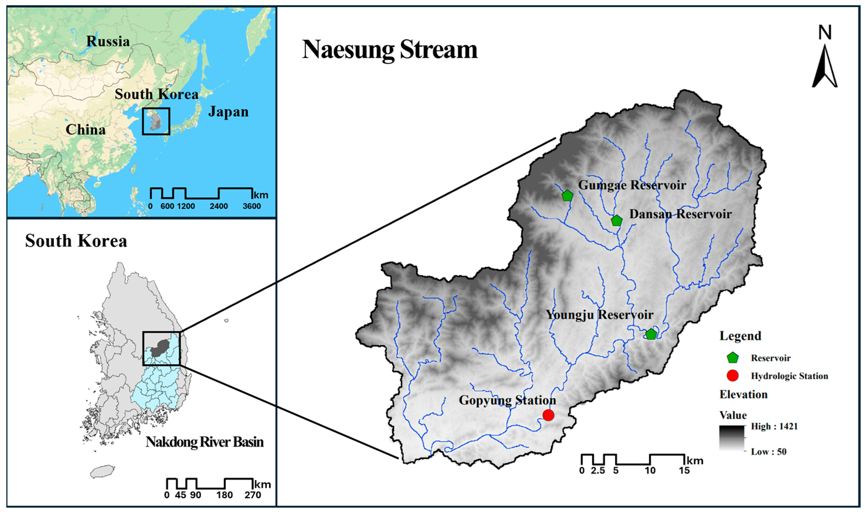
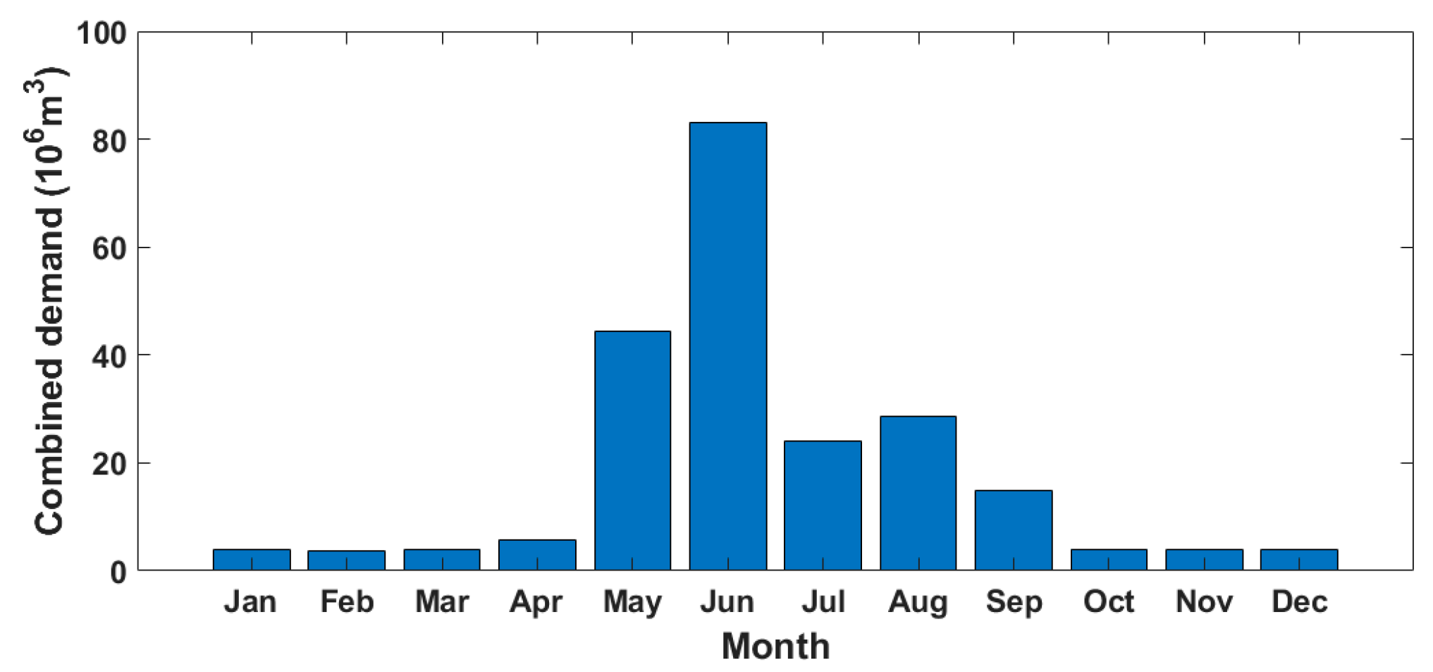
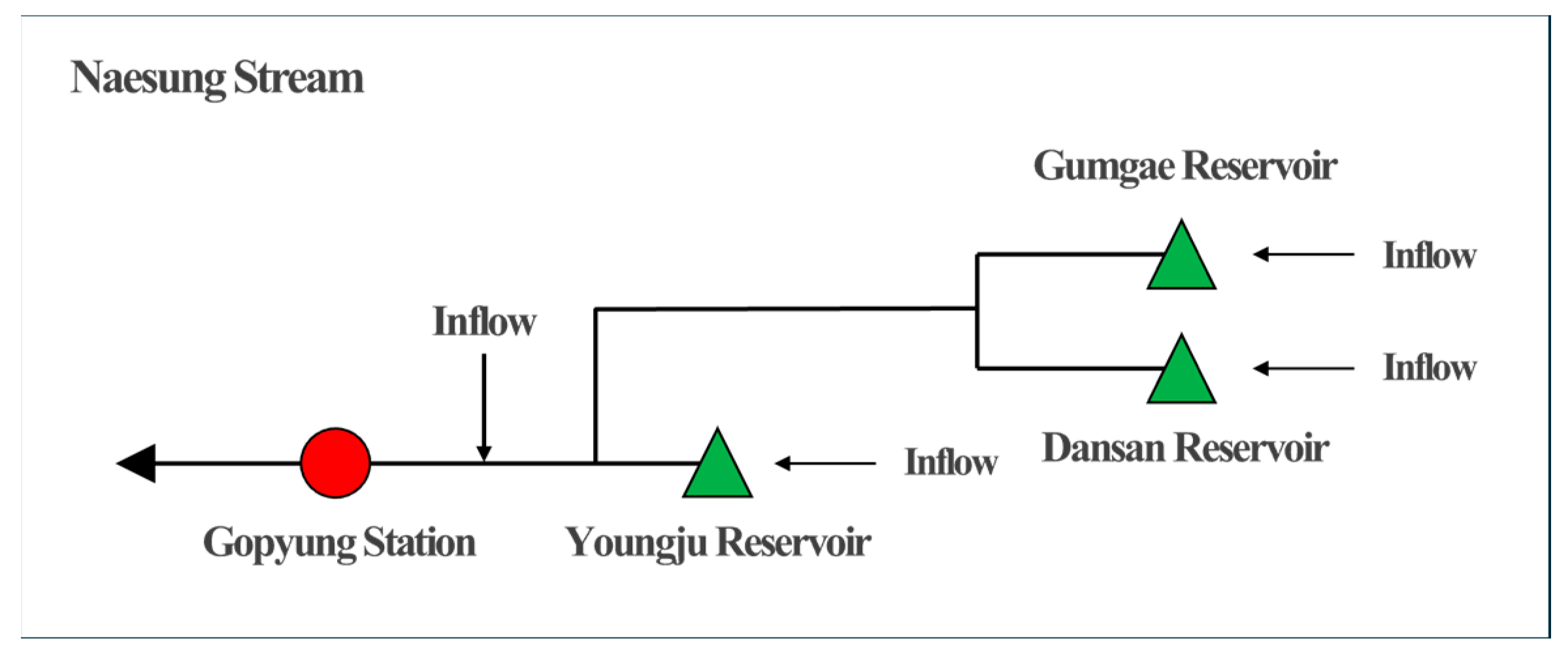
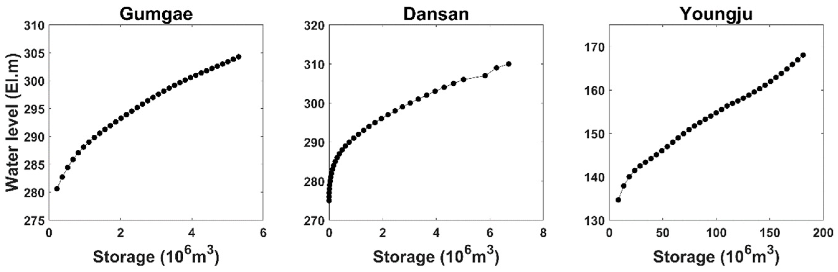
The Nakdong River Basin (Figure 1) is in the southeastern region of South Korea, with a channel length of 510.36 km. The watershed area of 23,384.21 km2 is the second largest watershed in South Korea. The Naesung Stream watershed, which is the study area, is located upstream of the Nakdong River. The watershed has a mainstream length of 110.69 km and an area of 1815.28 km2. The study area is characterized by a substantial proportion of rice fields within its total area and experiences a peak irrigation season in May and June. Therefore, the demand in the basin shown in Figure 2 was concentrated in May and June, owing to agricultural water usage. The Youngju (YJ) reservoir, the largest reservoir in the Naesung Stream watershed, was built in 2016. It contains 1.8 × 10⁸ m3 of storage capacity and was designed for water supply and flood control. There are 12 small-scale reservoirs in the Naesung Stream Basin, excluding the YJ reservoir. This study used only the Gumgye (GG) and Dansan (DS) reservoirs, which have a storage capacity of more than 5 million m3. The specifications of the GG, DS, and YJ reservoirs are listed in Table 2. The active storage capacity of the YJ reservoir is approximately 30 times larger than that of the other two reservoirs and maintains an average storage rate of 41.8%. As shown in the schematic of the reservoir system in Figure 3, the three reservoirs are connected parallelly. The released flow of each reservoir was combined with the inflow to the Gopyung station, which was the selected point to compare the ecological flows. The water-level storage curves of the three reservoirs shown in Figure 4 were used to convert the reservoir storage volume to the water level. Thus, the operation of a reservoir can be expressed as a change in water level.
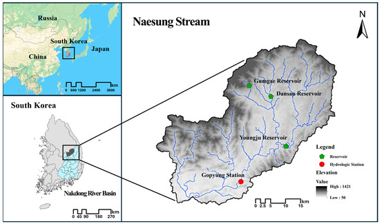
Figure 1.
Location of study area.

Figure 2.
The monthly combined domestic, industrial, and agricultural water demands.
Table 2.
Characteristics of reservoirs in the study area.
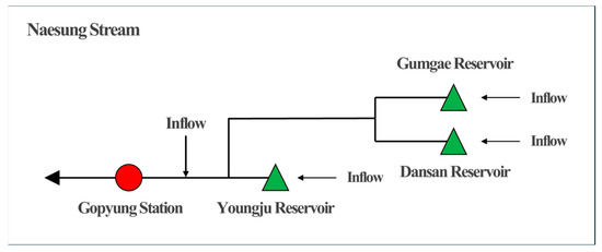
Figure 3.
Schematic of the reservoir system used in this study.
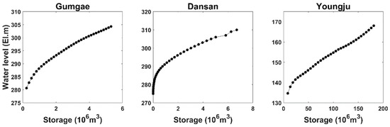
Figure 4.
Water-level storage curves for Gumgae, Dansan, and Youngju reservoirs.
2.2. Inflow Generation Using the SWAT Model
Accurate knowledge of reservoir inflow is important for optimizing reservoir operations. However, the observed inflows into small-scale reservoirs are limited. Therefore, it is necessary to predict the inflow to the reservoir. This study employed the Soil and Water Assessment Tool (SWAT) model to predict four inflows, including three inflows into each of the selected reservoirs and the inflow to the Gopyung station from the downstream watershed of the three reservoirs. In addition, the predicted downstream flow was used as input data to calculate the ecological flow.
The SWAT serves as a physical-based, semi-distributed, and continuous-time model [50]. Topographical, meteorological, and streamflow data were used to construct a SWAT model for the Naesung Stream watershed. The land surface elevation, soil type, and land use within the watershed were incorporated into the topography and soil information of the model. The meteorological data that served as the foundation for the SWAT model included daily rainfall, maximum and minimum temperatures, wind speed, and relative humidity from 2007 to 2014. The observed daily streamflow at Gopyung station from 2007 to 2014, before the construction of the YJ reservoir, was used to calibrate the SWAT model. The additional data sources used to build the model are listed in Table 3. The Nash–Sutcliffe efficiency (NSE), root mean standard deviation ratio (RSR), and coefficient of determination (R2) were employed to evaluate the performance of the SWAT model. The equations for each factor are given by Equations (1)–(3). The estimated daily flow at the Gopyung station was converted to monthly flow and used as input data to calculate the ecological flow.
where is the ith observed data point; is the ith simulated data point; is the mean of the observed data; is the mean of the simulated data point; and n is the total number of observed data points.
Table 3.
Input data sources in the SWAT model.
2.3. Calculation of Ecological Flow
This study used the flow duration curve (FDC)-shifting approach to estimate the ecological flow in an Environmental Management Class (EMC). The EMC was hierarchically arranged with six progressive levels from A to F. As the EMC advanced from F to A, a more stringent ecological flow was required to maintain this class. Detailed descriptions of each level are presented by the Department of Water Affairs and Forestry [51], Acreman and Dunbar [52], and Smakhtin and Eriyagama [53]. The FDC-shifting approach comprises three steps for estimating the ecological flow. The first step was to calculate the representative FDC using the streamflow. Subsequently, the FDCs of each EMC were shifted by one-step smaller percentiles than the representative percentile by 17 fixed percentiles of 0.01, 0.1, 1, 5, 10, 20, 30, 40, 50, 60, 70, 80, 90, 95, 99, 99.9, and 99.99%. For example, a streamflow with a 99.9% probability of exceedance in the representative curve corresponds to a probability of exceedance of 99% in class A, shifted by one step. The ecological flow of each component was determined after establishing an FDC for each EMC. This study utilizes the Global Environmental Flow Calculator (GEFC 2.0) to facilitate a more streamlined and simplified execution of this series of processes [54]. The stream flow at the Gopyung station, simulated by the SWAT model, was used as the input in the GEFC.
2.4. The Operation Model for Parallel Reservoirs
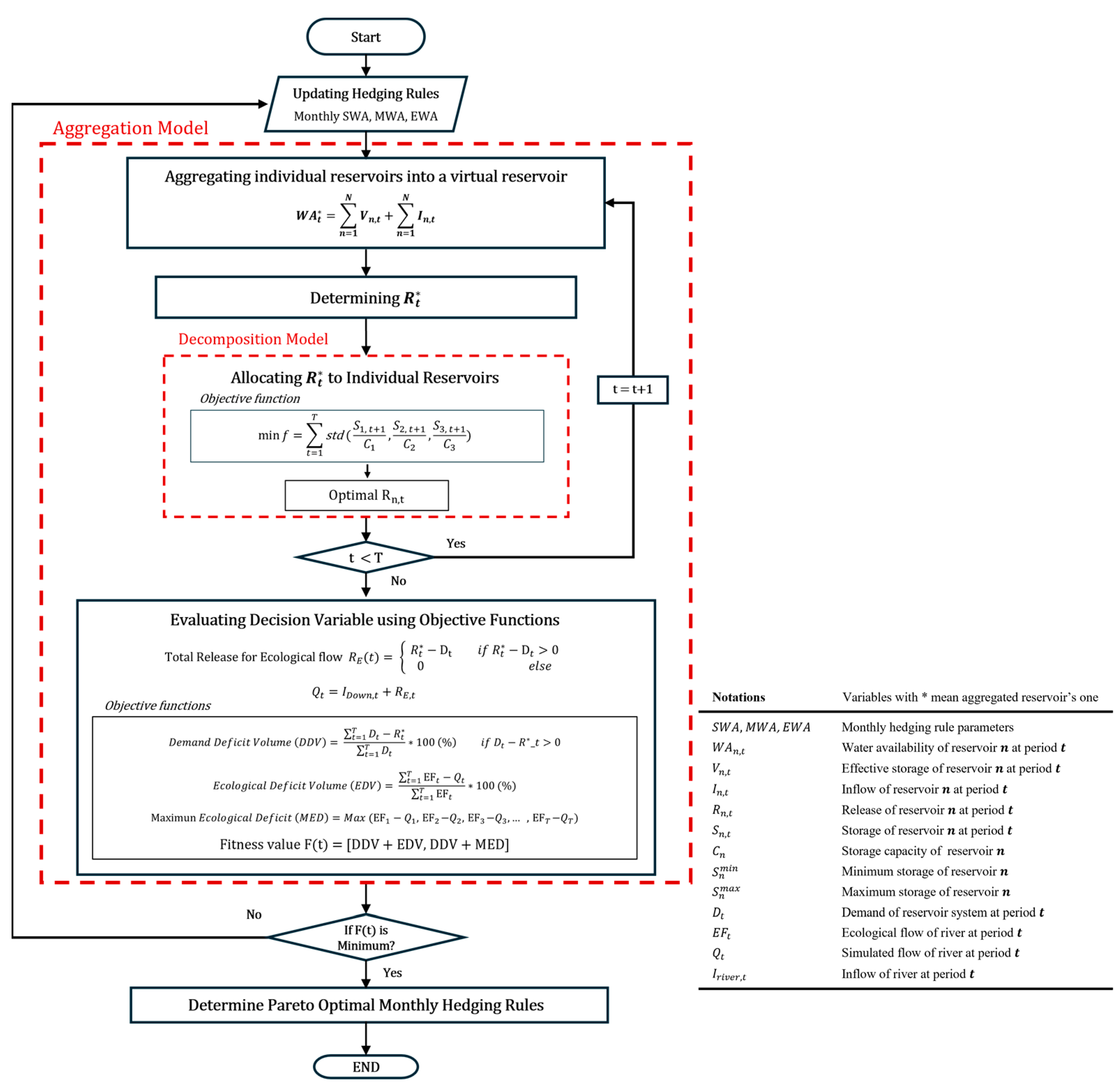
This study optimized the hedging rule for the joint operation of parallel reservoirs based on the AGDP method, as shown in the flowchart in Figure 5. The aggregation model determined the total release of the integrated individual reservoirs using hedging-rule curves. The decomposition model distributes the total release to individual reservoirs. In this study, the aggregation model optimized the monthly operating rules to maximize the efficiency of securing both the combined water demand and ecological flow. The second optimization in the decomposition model was used to select the proper distribution rate of the total release.
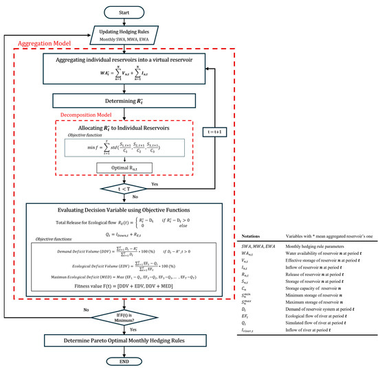
Figure 5.
The approach of aggregation and decomposition methods in this study.
This study used improved hedging rules for reservoir operations to release the ecological flow, which is an aggregated hedging rule for ecological flow (AHRE). The basic hedging rule parameters, SWA and EWA, were modified by incorporating MWA to allow separate control of the release of the combined water demand and ecological flow. This study compared the AHRE with the standard operation policy (SOP) and transformed the hedging rule (THR) to evaluate the effectiveness of the AHRE in parallel reservoir operations.
2.4.1. The Aggregation Model
The aggregation model calculates the total discharge based on the water availability of the aggregated virtual reservoir, which is defined as
where is the water availability of the parallel reservoir system in period t, is the storage volume excluding flows below the dead level of the reservoir n in period t, is the inflow to the reservoir n in period t, and N is the total number of reservoirs.
Standard Operation Policy (SOP)
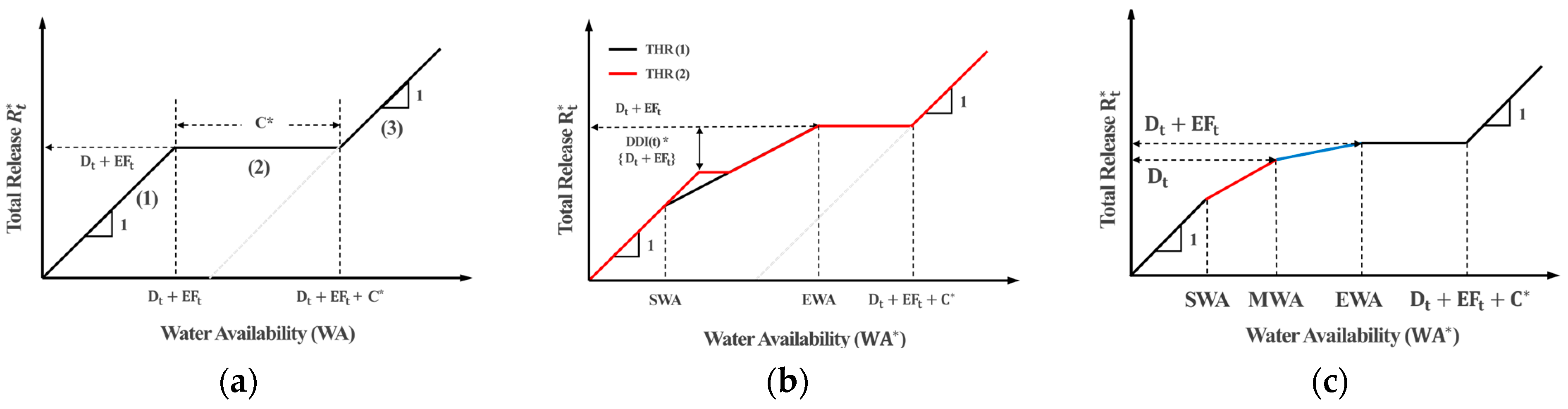
The SOP is a representative reservoir operation rule designed to minimize the effects of current droughts. The SOP method is characterized by maximizing the satisfaction of current water demand without considering the possibility of future shortages. However, this can lead to widespread shortages in the future [54,55]. The entire release of the reservoir system is contingent on the total demand, which comprises the combined water demand and ecological flow. As shown in Figure 6a, if is less than the total demand, all is released. Otherwise, if the remaining is greater than the active storage of the aggregated reservoir, even after releasing as much water as the total demand, an overflow will occur. Except, in this case, the aggregated reservoir releases as much water as possible of the total demand.
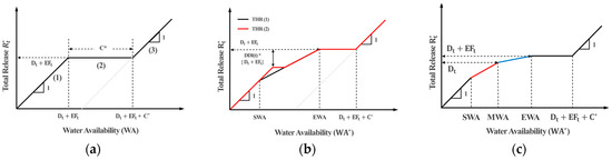
Figure 6.
Operation rules used in this study: (a) SOP; (b) THR; and (c) AHRE.
Transformed Hedging Rule (THR)
Over the past few decades, several studies have been conducted on modified HRs that incorporate various factors to achieve improved results [29,56,57,58]. Tan et al. [46] applied the damage depth index (DDI) to basic hedging rules to mitigate drought damage so that the release for demand was maximized when the DDI was closer to zero and minimized when the DDI approached one. This study applied the THR, a modified version of the method suggested by Tan et al. [46], for comparison. As illustrated in Figure 6b, the THRs contain two hedging rule cases: Case I occurs when and Case II occurs when :
Case I:
Case II:
where is the release of the aggregated reservoir in period t; and are the starting and ending water availabilities in period t; is the total demand, which comprises the combined water demand and ecological flow in period t; is the damage depth index in period t; and is the storage capacity of the aggregated reservoir in period t.
The objective functions of this study were the combined water demand deficit volume (DDV), ecological flow deficit volume (EDV), and maximum ecological flow deficit (MED). The DDV was calculated as the ratio of the total deficit volume to the total demand.
The cumulative discharge of the three reservoirs met the demand, and any surplus was directed downstream. The surplus is integrated with the inflow to the Gopyung station simulated by the SWAT model, which is given by Equations (8) and (9). By comparing the integrated discharge with the ecological flow, the EDV and MED were calculated as follows:
where is the discharge used to secure ecological flow out of the total release of reservoirs in period t; is the combined water demand in period t; is the inflow to the Gopyung station from the downstream watershed of the reservoirs in period t; is the streamflow at the Gopyung station in period t; EDV is the ecological flow deficit volume, which is calculated as the ratio of the total deficit volume to the total ecological flow; is the ecological flow at the Gopyung station in period t; T is the number of operation periods; and MED is the maximum ecological flow deficit, which is the largest deficit that occurred in a month.
The two objective functions are as follows:
A model of parallel reservoir operations must adhere to the following constraints:
- Water-balance constraints:
- Storage constraints:
- Release constraints:
- Hedging rule constraints:where is the storage of an individual reservoir n in period t; is the inflow of an individual reservoir n in period t; is the release of an individual reservoir n in period t, and is the minimum storage of an individual reservoir n; is the maximum storage of individual reservoir n; is the minimum storage and release of an individual reservoir n; and is the maximum release of an individual reservoir n.
Aggregated Hedging Rule for Ecological Flow (AHRE)
This study added the MWA factor to the basic hedging rule parameter to directly consider the ecological flow during reservoir operations. As shown in Figure 6c, when the WA of the aggregated reservoir is less than that of the MWA, only a portion of the combined water demand is satisfied. However, when the WA of the aggregated reservoir increases between the EWA and MWA, the aggregated reservoir is deemed to have the capacity to satisfy the entire water demand, as well as a portion of the ecological flow. A more detailed operating rule is defined as follows:
where is the middle water availability in period t.
The objective functions of this method are identical to those of the THRs. The following equations represent the constraints of this method:
- Water-balance constraints:
- Hedging rule constraints:
2.4.2. The Decomposition Model
The decomposition model distributes the total release, which is determined using the aggregation model described in Section 2.4.1. When parallel reservoirs are operated using the SOP and THR methods, the total release is distributed according to the ratio of the WA of each reservoir to the aggregated WA as follows:
where is the water availability of reservoir n in period t.
Unlike the two previously described methods, a distribution method based on optimization algorithms was applied to the AHRE. The objective function for reservoir optimization typically comprises the benefits derived from the released volume and the remaining storage (i.e., carryover storage). A decomposition model was employed to maximize the carryover storage for each reservoir. This model aimed to maintain storage rates across all reservoirs, which were as closely aligned as feasible throughout each period. Consequently, it is possible to minimize the water shortage and overflow of each reservoir while maximizing the efficiency of reservoir-system operations. The objective function minimizes the standard deviation between the storage rates of each reservoir after release as follows:
where SDS is the standard deviation between the storage rate of each reservoir after release and is the storage capacity of an individual reservoir n.
F = minimize SDS
The constraints of the decomposition model are represented as follows:
- Storage constraints:
- Release constraints:
- Decomposition constraints:
This study satisfied the constraints of the aggregation model (Equations (20)–(23)) and the decomposition model (Equations (27)–(29)).
3. Results
3.1. Inflow Estimation Using the SWAT Model
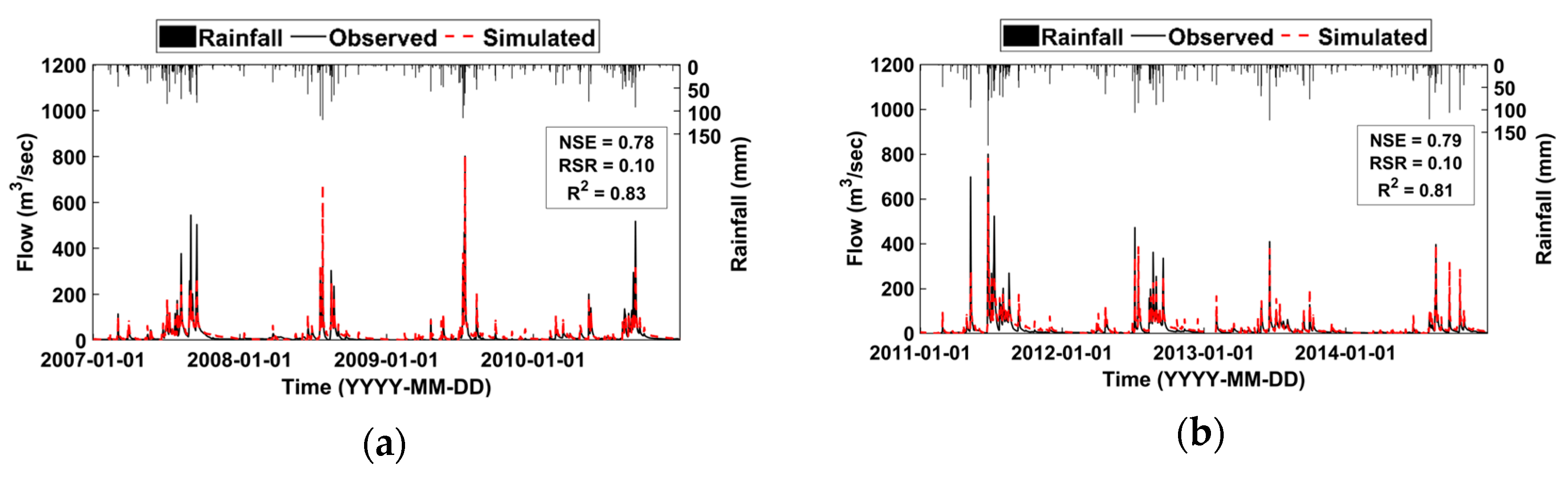
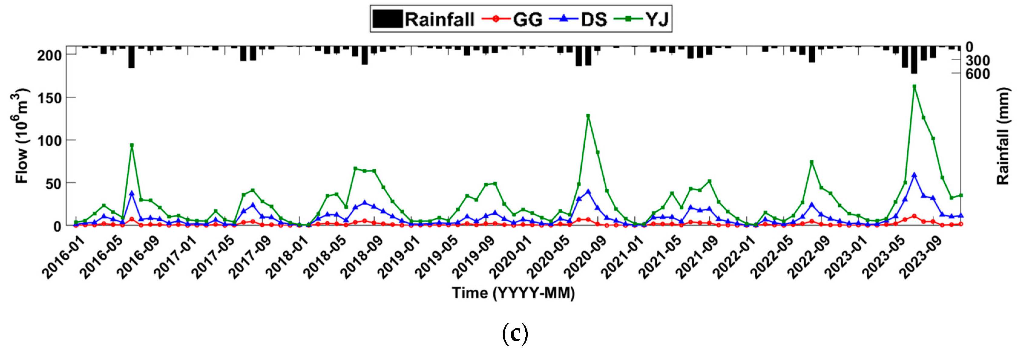
The SWAT model was used to estimate the inflow of each reservoir and Gopyung station. As mentioned in Section 2.2, the simulated streamflow between 2007 and 2014 was calibrated. The observed and simulated flows for each calibration and validation period are shown in Figure 7a and Figure 7b, respectively. The NSE, RSR, and R2 values were 0.78, 0.10, and 0.82 during the calibration period. During the validation period, the NSE, RSR, and R2 values were 0.79, 0.10, and 0.81, respectively, similar to the calibration period results. The estimated inflow for each reservoir is shown in Figure 7c.
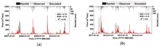
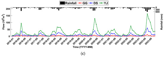
Figure 7.
Results of SWAT model: (a) comparison of observed and simulated flow in the calibration period (2007–2010); (b) comparison of observed and simulated flow in the validation period (2011–2014); (c) estimated reservoir inflows.
3.2. Ecological Flow Estimation
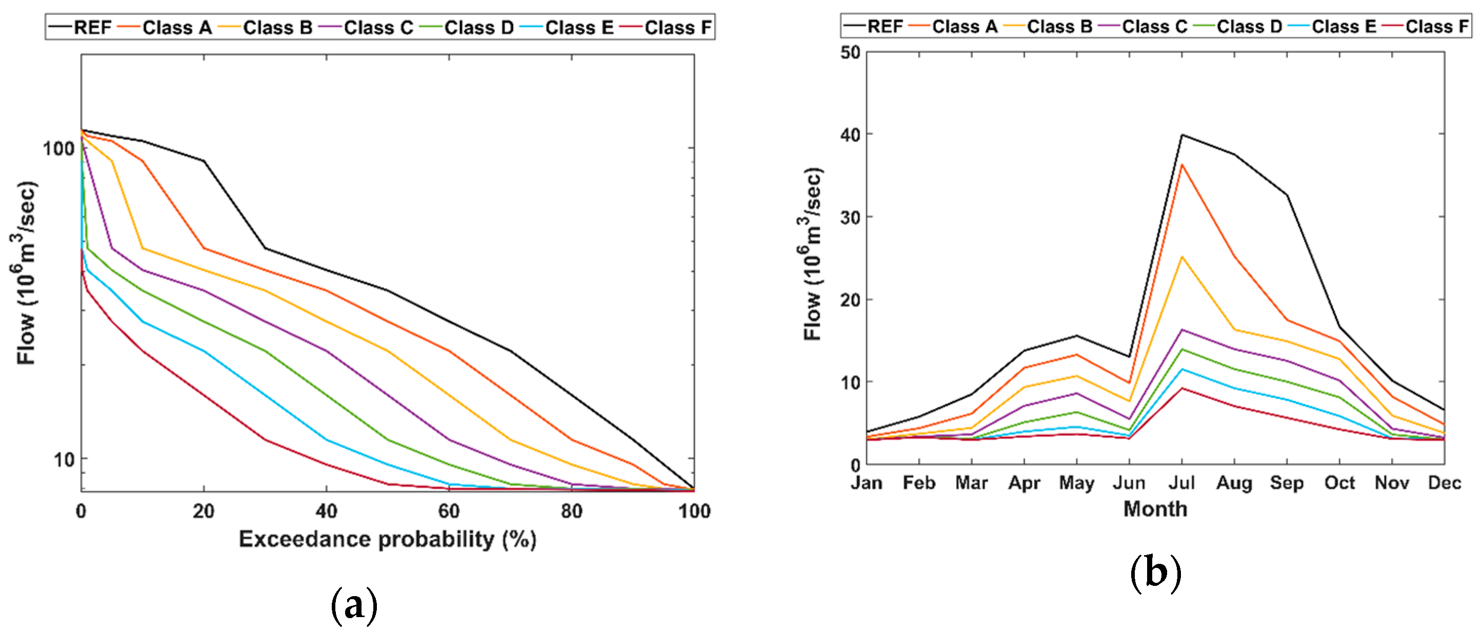
In this study, the monthly ecological flow was calculated using the FDC-shifting approach for different EMCs. The daily simulated flow from 2007 to 2015 was used instead of the observed streamflow, owing to numerous instances of missing data. The daily flow was converted into monthly data and applied to the GEFC software. The calculated FDCs and monthly averaged ecological flows are shown in Figure 8. This study adopted the largest ecological flow for EMC Class A to assess the effectiveness of the operation method in preserving the ecological flow.
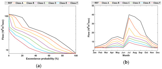
Figure 8.
Ecological flow estimation results under difference EMCs: (a) flow duration curves of ecological flow; (b) monthly averaged ecological flow.
3.3. Results of the Optimized AHRE Model
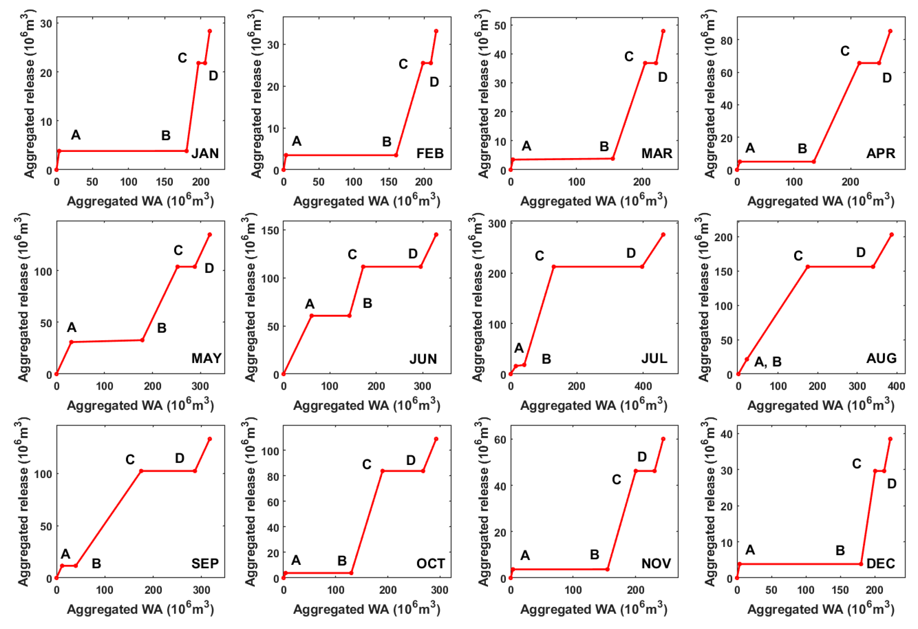
The estimated inflows and ecological flows were used to optimize the parallel reservoirs during 2016–2023. In the AHRE model, the two objective functions mentioned in THR Section are applied to find the Pareto optimal sets of decision variables: SWA, MWA, and EWA (three variables per month). The 36 variables of the AHRE model were optimized using the non-dominated sorting genetic algorithm (NSGA) II with the parameters listed in Table 4. The final Pareto fronts were distributed within 0.5% of the average of each objective function. Therefore, the optimal solution converged to a single point, and the average of each Pareto set was used as the optimal solution. Figure 9 presents the optimal monthly hedging-rule curves.
Table 4.
Parameters of NSGA II.

Figure 9.
Optimal monthly hedging-rule curves of the aggregated reservoir. A: SWA, B: MWA, C: EWA, D: C + D + EF.
The horizontal axis in Figure 9 represents the WA of the aggregated reservoir, and the vertical axis denotes the aggregated release of the parallel reservoir system. The curves were delineated using four key points, excluding the initial and terminal points. Point A, situated at the coordinates (SWA, SWA), marks the inception of hedging for the combined water demand. Similarly, Point B, positioned at (MWA, D), denotes the initiation of the hedging for ecological flow. The x-coordinates of Points C and D are EWA and C + D + EF, respectively, both of which share the same y-coordinate, D + EF. When the WA of the aggregated reservoir fell within the range delineated by Points A and B, a portion of the combined water demand was released. Between Points B and C, allocations were designated for both the combined water demand and a portion of the ecological flow. The aggregated release remained constant between points C and D, with the spillage commencing from Point D onwards. Figure 9 illustrates the various attributes of the monthly optimized hedging rules. The SWA demonstrated a pattern parallel to the magnitude of the combined water demand. However, the EWA tended to increase when the sum of the total demand and environmental flows was greater than that of the inflow. Notably, as the total water shortage escalated, the MWA approached the EWA more closely than the SWA. In June, which was marked by the most acute shortage, the disparity between the MWA and EWA was less than 30 million m3. However, in August, which was characterized by the highest water availability, the gap widened to over 150 million m3. The change in the spacing was derived from the distinct characteristics of the AHRE method. As the MWA approached the SWA, more water was released than when the basic hedging rules were applied, and as the MWA approached the EWA, less water was discharged. Figure 9 illustrates the pivotal function of the hedging rule parameters SWA, MWA, and EWA in optimizing the reservoir operation to ensure ecological flow.
3.4. Comparison of the Three Operating Models
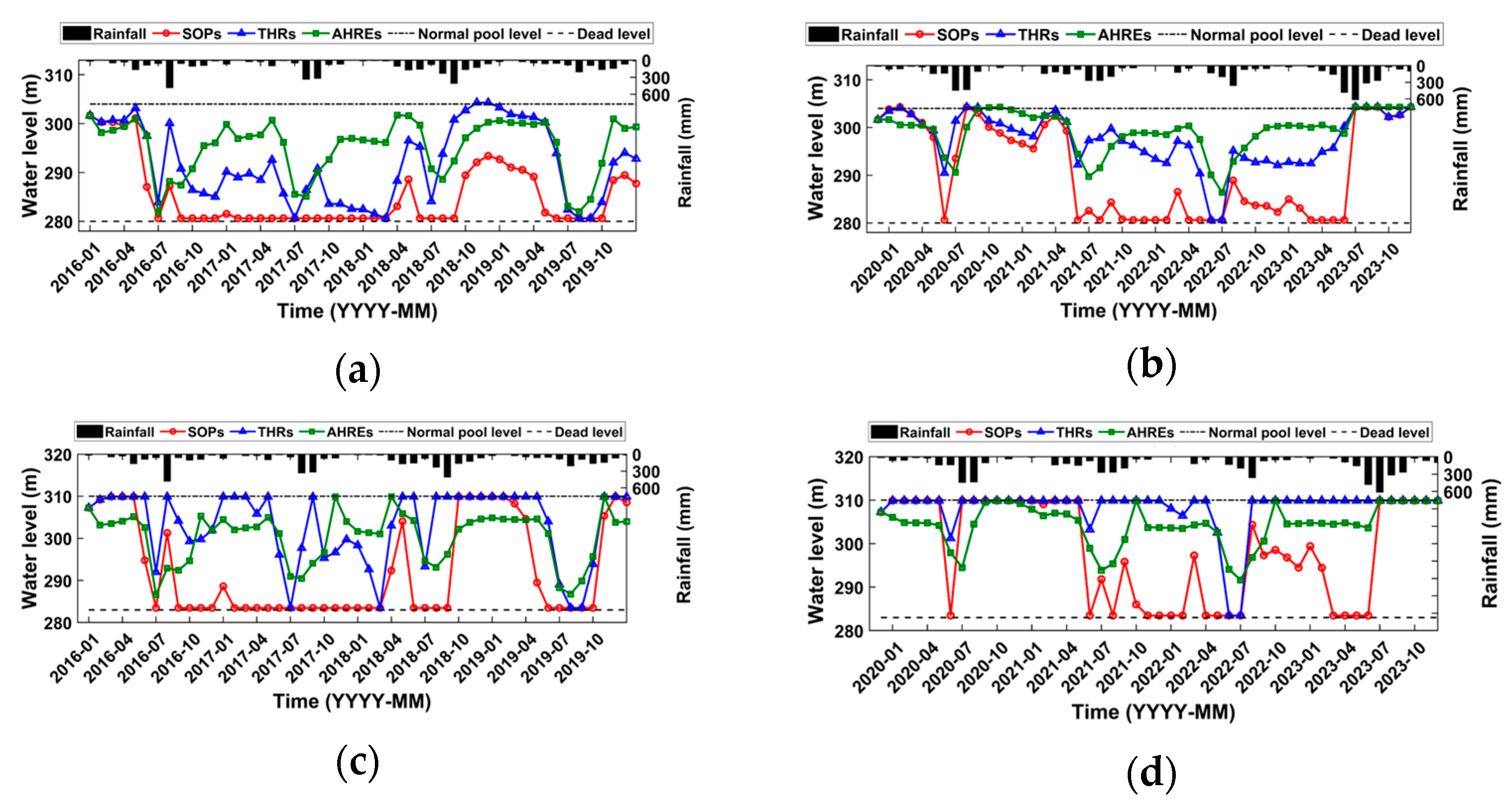
The operational results of the AHREs, SOPs, and THRs were compared to evaluate their effectiveness. The water levels of each reservoir during the training period (2016–2019) and testing period (2020–2023) using the three methods are plotted in Figure 10. Under the SOPs, most reservoirs maintained low water levels close to dead water levels. The implementation of THRs resulted in the DS reservoir approaching a normal pool level. However, the water level of the YJ reservoir was relatively close to the dead water level. The water levels of reservoirs GG and YJ in the AHREs were relatively higher than those of the SOPs and THRs. As shown in Figure 10c,d, when the AHREs were applied, the water-level change patterns of each reservoir were similar. In contrast, the water level of the DS reservoir using the SOPs and THRs increased and then decreased more rapidly than that of the other reservoirs. This difference in water-level changes between the reservoirs was caused by the decomposition method. As shown in Figure 7c, the maximum inflow volumes of reservoirs GG and DS were 11.1 million m3 and 58.8 million m3, respectively, and the average inflow volumes were 1.6 million m3 and 9.6 million m3. On the other hand, the active storages of each reservoir were 5.3 million m3 and 6.2 million m3, which are small compared to the inflow values. In particular, the storage capacity of the DS reservoir was approximately 1.2 times greater than that of the GG reservoir. However, the inflow of the DS reservoir was approximately 4–400 times greater than that of the GG reservoir. The difference in the inflow and storage ratios between the reservoirs and the small size of the GG and DS reservoirs relative to the inflow pose difficulties in simply applying the ratios when constructing the decomposition model. For the SOPs and THRs, the aggregated release was distributed based on the WA of each reservoir. Therefore, the DS reservoir released a small portion of the aggregated release compared to its inflow. Consequently, the DS reservoir was more prone to overflow than the other reservoirs. However, in the AHREs, an objective function was used to ensure that the storage rates of the reservoirs were as similar as possible. Thus, the AHREs effectively operated the reservoir system by saving water without overflow. Furthermore, by maintaining similar water levels in each reservoir, they can effectively prepare for unexpected drought. Figure 10 demonstrates that AHREs provide more stable reservoir operations than the SOPs and THRs.
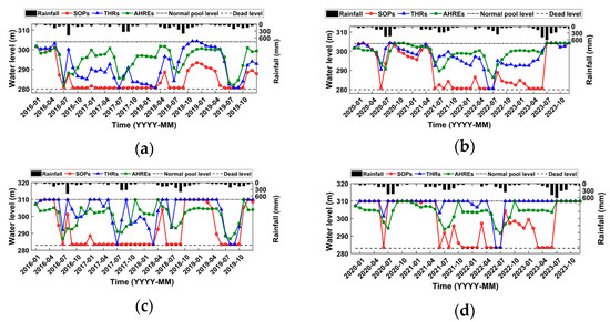
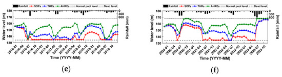
Figure 10.
Monthly water levels of reservoirs: (a) GG reservoir in the training period (2016–2019); (b) GG reservoir in the testing period (2020–2023); (c) DS reservoir in the training period; (d) DS reservoir in the testing period; (e) YJ reservoir in the training period; (f) YJ reservoir in the testing period.
Figure 11 shows a box plot of the water level of the SOPs. However, despite the relatively low average water level in the YJ reservoir compared to that of the AHREs, overflow occurred more frequently in the GG and DS reservoirs than in the AHREs. Especially, the DS reservoir maintained its normal pool level and overflowed for most of the period, resulting in the water-level distribution shown in Figure 11b being concentrated at 100%. Most research on water supply through reservoir operations primarily assesses the operational performance by relying solely on the demand deficit. However, to minimize the damage caused by the uncertainty of reservoir operation elements (e.g., unpredictably low inflow or high demand), the ability to store sufficient water to respond effectively to droughts is important, as stated by Draper and Lund (2004) [23]. According to their argument, the water-level distributions of each reservoir during the operation periods in Figure 11 indicate the adaptability of the AHREs to uncertainties.
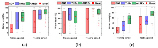
Figure 11.
Box plots of water level distribution of the three reservoirs in the training period (2016–2019) and testing period (2020–2023): (a) GG reservoir; (b) DS reservoir; (c) YJ reservoir.
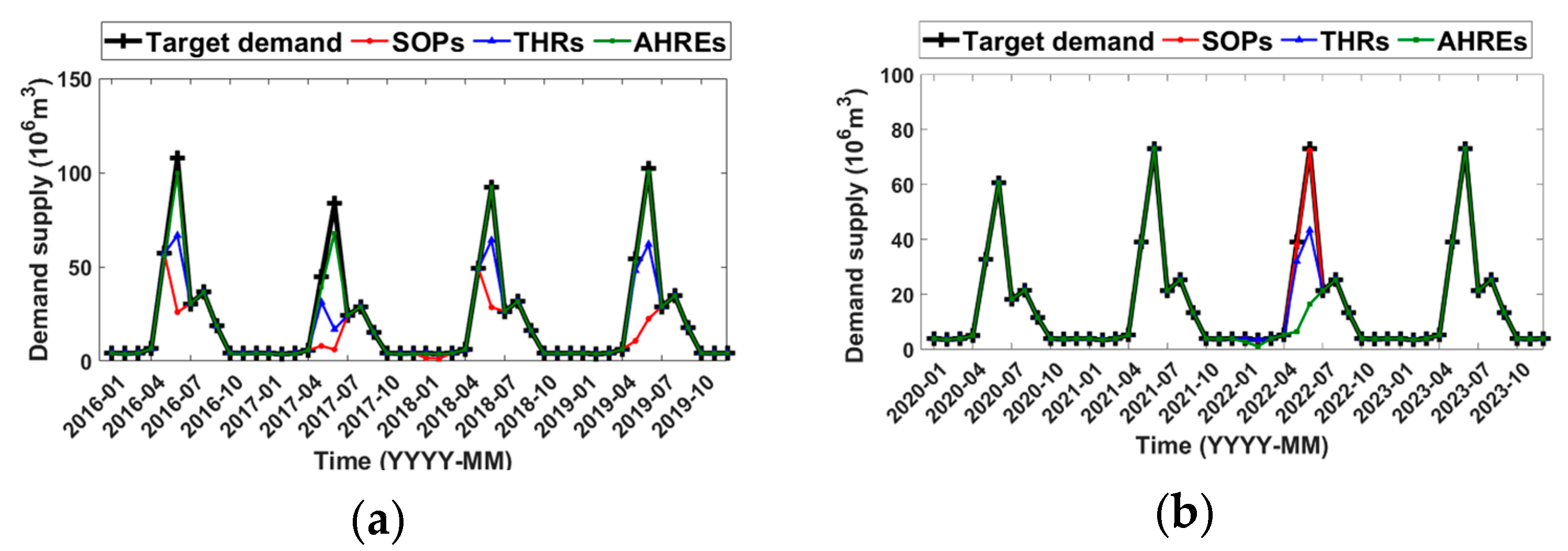
The monthly combined water demand supplied by each method is compared in Figure 12. During the training period, when the target demand was relatively high owing to low rainfall, only the AHREs showed a high satisfaction rate. In contrast, the other two methods had severe shortcomings. Shortages occurred, especially in June, when the demand was the highest. During the testing period, the supply of SOPs and THRs was not uniform, with extreme shortages occurring only in 2022, as shown in Figure 12b.
Figure 12.
Monthly combined water demand supply: (a) in the training period (2016–2019); (b) in the testing period (2020–2023).
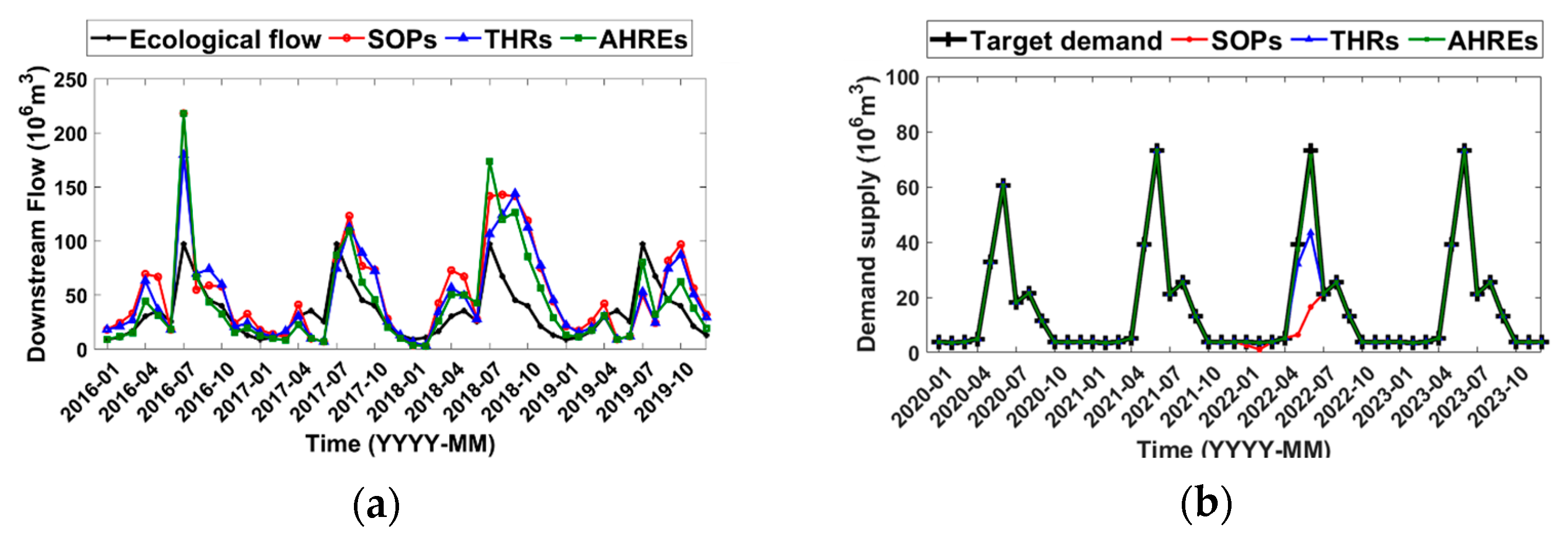
Figure 13 illustrates a comparison between the ecological and downstream flows, which encompass the remaining discharge after supplying the demand and inflow into the Gopyung station. The AHREs yielded better results in terms of ecological flow satisfaction than the other two methods during both the training and testing periods. According to Figure 13a, the downstream flow using the SOPs and THRs experienced a major shortage in May and June, when the water demand increased. The downstream flows of the SOPs and THRs almost meet the ecological flow during the testing period, except in May, June, and July 2022. The AHREs experienced small additional deficits in March, April, and May 2020. The water storage volume secured by the small deficit prevented a major drought from June to July 2022, with a sufficient water supply.
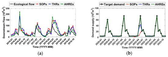
Figure 13.
Monthly flow at Gopyung station: (a) in the training period (2016–2019); (b) in the testing period (2020–2023).
Figure 12 and Figure 13 confirm that the AHRE method was superior in terms of both water demand and ecological flow supply. By adding the MWA factor, the AHREs met the existing demand. Applying the optimization model to distribute the discharge maintained high water storage in each reservoir by minimizing the waste of available water due to overflow.
4. Discussion
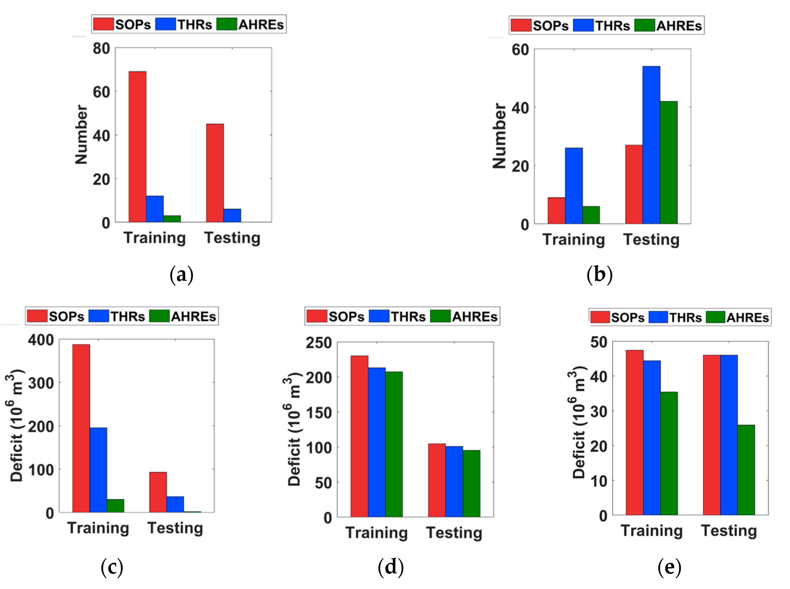
The assessment of reservoir operations requires a multifaceted approach. Previous research on reservoir operations for water supply has mainly focused on satisfying supply goals. However, in addition to simply maximizing satisfaction with the water demand and ecological flow, it is essential to evaluate the stability and sustainability of operations. Figure 14 presents an analysis of the efficiency of reservoir system operations from various perspectives. Figure 14a,b show the number of times each reservoir reached dead and normal pool levels, respectively. These two graphs depict the stability, sustainability, and resilience of the reservoir operation to uncertainty. Figure 14c–e illustrate the total water demand, total ecological flow, and MED, respectively. These three graphs illustrate the capacity of reservoir operations to meet supply and demand and respond to droughts. As shown in Figure 14a, under the SOPs, the three reservoirs reached dead levels 69 and 45 times during the training and testing periods, respectively. However, the three reservoirs reached normal pool levels only a few times. This result reflects the characteristics of the SOP method, which releases all available water to satisfy demand as much as possible. When using the AHRE method, the GG and YJ reservoirs were out of reach of the dead level, and the total number of reaches was very low. In the practical application of reservoir operations, the term ‘dead level’ extends beyond the conventional definition of the minimum reservoir level to the final line of defense, which must be essentially avoided. As mentioned in Section 3.4, utilizing the MWA factor enables a more conservative reservoir operation than the basic hedging rule. In Figure 8, the July–September hedging curves are similar to the basic hedging rule, with points A, B, and C located relatively linearly. Conversely, during the water-shortage period from November to March, the MWA approached the EWA, resulting in a significant curvature in the hedging curve. Minimizing dead and normal pool levels while meeting demand was possible because of the flexibility of the operating rules. However, AHREs showed low efficiency when relatively high rainfall occurred because its aim is drought adaptation. For this reason, the increased rate of the number of times the normal pool level is reached in the testing period, which has a relatively higher rainfall compared to the training period, was larger than that of the other two methods, as illustrated in Figure 14b. Figure 14c shows the DDV, representing the actual supply volume of the total combined water demand during the operational period. The SOPs were 37.8%, and the THRs were 19.1%, displaying significant values compared with 3.6% in AHREs during the training period. Similarly, the AHREs rarely experienced deficits during the testing period, whereas the SOP and THRs exhibited relatively high deficit ratios of 12% and 4.75%, respectively. As shown in Figure 14d, the AHRE method exhibited the smallest ecological flow deficit during both the training and testing periods. The AHREs also presented a smaller maximum ecological deficit than the SOPs and THRs. The characteristics of the AHRE method, which operates separately from demand and ecological flow, lead to direct control of the section that supplies only water demand and the section that releases water demand and ecological flow. However, in the case of the THRs, the release of ecological flow increased with the same slope as the release of water demand. Figure 14 demonstrates that AHREs outperform SOPs and THRs in terms of overall supply stability, with a deficit that is uniformly distributed throughout the year rather than concentrated in a specific month. The effectiveness of AHREs is evident from the number of times each reservoir reached dead and normal pool levels, as well as their ability to satisfy both demand and ecological flow.

Figure 14.
Comparison of operation performances among operation methods and observed flow during the training period (2016–2019) and testing period (2020–2023): (a) number of times each reservoir reached its dead level; (b) number of times each reservoir reached its normal pool level; (c) demand deficit volume; (d) ecological flow deficit volume; (e) maximum ecological flow deficit.
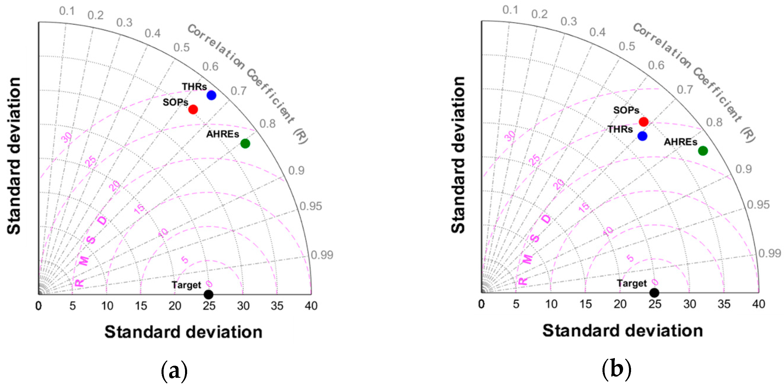
The optimal release strategy for reservoir operation presupposes maximizing water discharge and judicious operational management in line with ecological flow requirements. Figure 14d,e offer insights into the comparative reservoir performance but fall short of furnishing a comprehensive operational efficiency assessment across methodologies. Therefore, the Taylor diagram in Figure 15 was used to compare the ecological and downstream flows for each method. In Figure 15, the black-filled target circle denotes the ecological flow, and the colored circles represent the downstream flows obtained using the three methods. Three statistical metrics, namely standard deviation, correlation coefficients, and root mean square distance (RMSD), were elucidated within the Taylor diagram through spatial representations. The standard deviation was defined as the radial distance originating from the center of the diagram. The azimuthal angle within the quadrant conveys the correlation coefficient between the ecological and downstream flows for each of the three methods. The spatial distance between the target circle and the colored circles visually represents the RMSD. A closer proximity of the colored circles to the target point signifies a diminished RMSD, indicative of heightened concordance between downstream flow and ecological flow. In Figure 15a,b, the circle of the AHREs is the closest to the target circle. The correlation coefficient of the AHREs was the highest, and the RMSD of the AHREs was the lowest. This result shows that when the AHRE method was applied, the downstream flow was most similar to the ecological flow of the three methods. Consequently, Figure 15 unequivocally underscores the AHRE methodology as a furnishing judicious reservoir operation conducive to securing ecological flow and transcending the mere maximization of discharge.
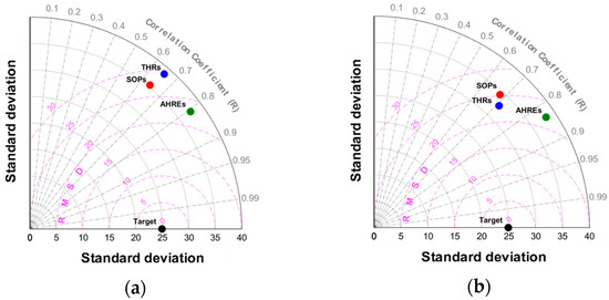
Figure 15.
Taylor diagram of ecological flow and downstream flow of three methods: (a) in the training period (2016–2019); (b) in the testing period (2020–2023).
5. Conclusions
This study proposes an AGDP method to optimize the hedging rules for three parallel reservoirs while considering ecological flow. By incorporating the MWA into the basic hedging rule parameters, the modified hedging rules can be applied to reservoir operations, enabling flexible reservoir operations. Two objective functions addressing the total water demand deficit, total ecological flow deficit, and MED were employed to meet conventional demand and ecological needs. The total discharge from the reservoirs was determined using monthly optimal hedging rules consisting of the SWA, MWA, and EWA. The decomposition model consisted of an optimization model that distributed the aggregated release to individual reservoirs to minimize the standard deviation of the post-discharge reservoir storage rates. A performance evaluation was conducted by comparing the proposed method with conventional operating rules, namely the SOP and THR methods. The SOPs and THRs allocate the total release to individual reservoirs based on their ratio of available water to the total aggregated system. The comparison results confirmed that the AHRE method is superior to the existing methods in terms of securing both water demand and ecological flow. In particular, its MED was significantly smaller than that of the other methods, indicating that a consistent and stable supply was possible. The water level changed in each reservoir when the AHRE method was applied, and each reservoir was operated within a small range of variation with a similar trend owing to decomposition through the optimization function. Thus, the number of times each reservoir reaches the dead and normal pool levels is minimized, enabling an effective response even in the event of a sudden drought.
This study evaluated the results of applying the optimal operating rule without knowing the input during the testing period. Similar to the results for the training period, the AHRE method showed excellent performance during the testing period, confirming its ability to respond to drought uncertainty. However, the fundamental problem of applying optimization to future inflows without considering forecast uncertainty has not yet been solved. Therefore, future research must add a method to determine the operation rate by considering the uncertainty of various input data, such as inflow and demand.
Author Contributions
Investigation and methodology, I.M.; data curation and investigation, N.L.; data curation and investigation, S.K., Y.B. and J.J.; supervision, K.J. and D.P. All authors have read and agreed to the published version of the manuscript.
Funding
This paper was supported by Konkuk University in 2024.
Institutional Review Board Statement
Not applicable.
Data Availability Statement
The data presented in this study are available on request from the corresponding author.
Conflicts of Interest
The authors declare no conflicts of interest.
Abbreviations
| AHRE | Aggregated hedging rule for ecological flow |
| AGDP | Aggregation–decomposition |
| SWAT | Soil and Water Assessment Tool |
| GEFC | Global Environmental Flow Calculator |
| EMC | Environmental Management Class |
| SOP | Standard operation policy |
| THR | Transformed hedging rule |
| DDV | Combined water demand deficit volume |
| EDV | Ecological flow deficit volume |
| MED | Maximum ecological flow deficit |
| NSGA | Non-dominated sorting genetic algorithm |
References
- Arthington, A.H.; Bunn, S.E.; Poff, N.L.; Naiman, R.J. The Challenge of Providing Environmental Flow Rules to Sustain River Ecosystems. Ecol. Appl. 2006, 16, 1311–1318. [Google Scholar] [CrossRef]
- Trenberth, K.E.; Dai, A.; van der Schrier, G.; Jones, P.D.; Barichivich, J.; Briffa, K.R.; Sheffield, J. Global Warming and Changes in Drought. Nat. Clim. Change 2014, 4, 17–22. [Google Scholar] [CrossRef]
- Walling, B.; Chaudhary, S.; Dhanya, C.T.; Kumar, A. Estimation of Environmental Flow Incorporating Water Quality and Hypothetical Climate Change Scenarios. Environ. Monit. Assess. 2017, 189, 225. [Google Scholar] [CrossRef]
- Chang, L.-C.; Chang, F.-J. Multi-Objective Evolutionary Algorithm for Operating Parallel Reservoir System. J. Hydrol. 2009, 377, 12–20. [Google Scholar] [CrossRef]
- Intergovernmental Panel on Climate Change (IPCC) Climate Change 2021—The Physical Science Basis: Working Group I Contribution to the Sixth Assessment Report of the Intergovernmental Panel on Climate Change, 1st ed.; Cambridge University Press: Cambridge, UK, 2023; ISBN 978-1-00-915789-6.
- Al-Jawad, J.Y.; Alsaffar, H.M.; Bertram, D.; Kalin, R.M. Optimum Socio-Environmental Flows Approach for Reservoir Operation Strategy Using Many-Objectives Evolutionary Optimization Algorithm. Sci. Total Environ. 2019, 651, 1877–1891. [Google Scholar] [CrossRef]
- Li, F.-F.; Wei, J.-H.; Fu, X.-D.; Wan, X.-Y. An Effective Approach to Long-Term Optimal Operation of Large-Scale Reservoir Systems: Case Study of the Three Gorges System. Water Resour. Manag. 2012, 26, 4073–4090. [Google Scholar] [CrossRef]
- Anand, J.; Gosain, A.K.; Khosa, R. Optimisation of Multipurpose Reservoir Operation by Coupling Soil and Water Assessment Tool (SWAT) and Genetic Algorithm for Optimal Operating Policy (Case Study: Ganga River Basin). Sustainability 2018, 10, 1660. [Google Scholar] [CrossRef]
- Yang, Z.; Yang, K.; Hu, H.; Su, L. The Cascade Reservoirs Multi-Objective Ecological Operation Optimization Considering Different Ecological Flow Demand. Water Resour. Manag. 2019, 33, 207–228. [Google Scholar] [CrossRef]
- Li, F.-F.; Shoemaker, C.A.; Qiu, J.; Wei, J.-H. Hierarchical Multi-Reservoir Optimization Modeling for Real-World Complexity with Application to the Three Gorges System. Environ. Model. Softw. 2015, 69, 319–329. [Google Scholar] [CrossRef]
- Sedighkia, M.; Abdoli, A. Design of Optimal Environmental Flow Regime at Downstream of Multireservoir Systems by a Coupled SWAT-Reservoir Operation Optimization Method. Environ. Dev. Sustain. 2023, 25, 834–854. [Google Scholar] [CrossRef]
- Al-Aqeeli, Y.H.; Mahmood Agha, O.M.A. Optimal Operation of Multi-Reservoir System for Hydropower Production Using Particle Swarm Optimization Algorithm. Water Resour. Manag. 2020, 34, 3099–3112. [Google Scholar] [CrossRef]
- Pan, Z.; Chen, L.; Teng, X. Research on Joint Flood Control Operation Rule of Parallel Reservoir Group Based on Aggregation–Decomposition Method. J. Hydrol. 2020, 590, 125479. [Google Scholar] [CrossRef]
- Dobson, B.; Wagener, T.; Pianosi, F. An Argument-Driven Classification and Comparison of Reservoir Operation Optimization Methods. Adv. Water Resour. 2019, 128, 74–86. [Google Scholar] [CrossRef]
- Clark, E.J. Impounding Reservoirs. J. (Am. Water Work. Assoc.) 1956, 48, 349–354. [Google Scholar]
- Oliveira, R.; Loucks, D.P. Operating Rules for Multireservoir Systems. Water Resour. Res. 1997, 33, 839–852. [Google Scholar] [CrossRef]
- T. Bower, B.; M. Hufschmidt, M.; W. Reedy, W. 11. Resource Systems by Simulation Analyses. In Design of Water-Resource Systems; Harvard University Press: Cambridge, MA, USA, 1962; pp. 443–458. ISBN 978-0-674-42103-5. [Google Scholar] [CrossRef]
- Revelle, C.; Joeres, E.; Kirby, W. The Linear Decision Rule in Reservoir Management and Design: 1, Development of the Stochastic Model. Water Resour. Res. 1969, 5, 767–777. [Google Scholar] [CrossRef]
- Maass, A.; Hufschmidt, M.M.; Dorfman, R.; Thomas, H.A., Jr.; Marglin, S.A.; Fair, G.M. Design of Water-Resource Systems: New Techniques for Relating Economic Objectives, Engineering Analysis, and Governmental Planning; Harvard University Press: Cambridge, MA, USA, 1962; ISBN 978-0-674-42103-5. [Google Scholar] [CrossRef]
- Stedinger, J.R.; Sule, B.F.; Loucks, D.P. Stochastic Dynamic Programming Models for Reservoir Operation Optimization. Water Resour. Res. 1984, 20, 1499–1505. [Google Scholar] [CrossRef]
- Bayazit, M.; Ünal, N.E. Effects of Hedging on Reservoir Performance. Water Resour. Res. 1990, 26, 713–719. [Google Scholar] [CrossRef]
- Shih, J.; ReVelle, C. Water-Supply Operations during Drought: Continuous Hedging Rule. J. Water Resour. Plann. Manag. 1994, 120, 613–629. [Google Scholar] [CrossRef]
- Draper, A.J.; Lund, J.R. Optimal Hedging and Carryover Storage Value. J. Water Resour. Plann. Manag. 2004, 130, 83–87. [Google Scholar] [CrossRef]
- Shiau, J. Analytical Optimal Hedging with Explicit Incorporation of Reservoir Release and Carryover Storage Targets. Water Resour. Res. 2011, 47, 2010WR009166. [Google Scholar] [CrossRef]
- Ahmadianfar, I.; Zamani, R. Assessment of the Hedging Policy on Reservoir Operation for Future Drought Conditions under Climate Change. Clim. Change 2020, 159, 253–268. [Google Scholar] [CrossRef]
- Kang, L.; Zhang, S.; Ding, Y.; He, X. Extraction and Preference Ordering of Multireservoir Water Supply Rules in Dry Years. Water 2016, 8, 28. [Google Scholar] [CrossRef]
- Azari, A.; Hamzeh, S.; Naderi, S. Multi-Objective Optimization of the Reservoir System Operation by Using the Hedging Policy. Water Resour. Manag. 2018, 32, 2061–2078. [Google Scholar] [CrossRef]
- Abdollahi, A.; Ahmadianfar, I. Multi-Mechanism Ensemble Interior Search Algorithm to Derive Optimal Hedging Rule Curves in Multi-Reservoir Systems. J. Hydrol. 2021, 598, 126211. [Google Scholar] [CrossRef]
- Huang, C.; Zhao, J.; Wang, Z.; Shang, W. Optimal Hedging Rules for Two-Objective Reservoir Operation: Balancing Water Supply and Environmental Flow. J. Water Resour. Plann. Manag. 2016, 142, 04016053. [Google Scholar] [CrossRef]
- Xu, W. Study on Multi-Objective Operation Strategy for Multi-Reservoirs in Small-Scale Watershed Considering Ecological Flows. Water Resour. Manag. 2020, 34, 4725–4738. [Google Scholar] [CrossRef]
- Ahmadianfar, I.; Bozorg-Haddad, O.; Chu, X. Optimizing Multiple Linear Rules for Multi-Reservoir Hydropower Systems Using an Optimization Method with an Adaptation Strategy. Water Resour. Manag. 2019, 33, 4265–4286. [Google Scholar] [CrossRef]
- Ahmadianfar, I.; Kheyrandish, A.; Jamei, M.; Gharabaghi, B. Optimizing Operating Rules for Multi-Reservoir Hydropower Generation Systems: An Adaptive Hybrid Differential Evolution Algorithm. Renew. Energy 2021, 167, 774–790. [Google Scholar] [CrossRef]
- Dariane, A.B.; Momtahen, S. Optimization of Multireservoir Systems Operation Using Modified Direct Search Genetic Algorithm. J. Water Resour. Plann. Manag. 2009, 135, 141–148. [Google Scholar] [CrossRef]
- Ahmadi Najl, A.; Haghighi, A.; Vali Samani, H.M. Simultaneous Optimization of Operating Rules and Rule Curves for Multireservoir Systems Using a Self-Adaptive Simulation-GA Model. J. Water Resour. Plann. Manag. 2016, 142, 04016041. [Google Scholar] [CrossRef]
- Rashid, M.U.; Latif, A.; Azmat, M. Optimizing Irrigation Deficit of Multipurpose Cascade Reservoirs. Water Resour. Manag. 2018, 32, 1675–1687. [Google Scholar] [CrossRef]
- Wang, Z.; Zhang, L.; Cheng, L.; Liu, K.; Ye, A.; Cai, X. Optimizing Operating Rules for a Reservoir System in Northern China Considering Ecological Flow Requirements and Water Use Priorities. J. Water Resour. Plann. Manag. 2020, 146, 04020051. [Google Scholar] [CrossRef]
- Deep, K.; Singh, K.P.; Kansal, M.L.; Mohan, C. Management of Multipurpose Multireservoir Using Fuzzy Interactive Method. Water Resour. Manag. 2009, 23, 2987–3003. [Google Scholar] [CrossRef]
- Wang, Y.; Chang, J.; Huang, Q. Simulation with RBF Neural Network Model for Reservoir Operation Rules. Water Resour. Manag. 2010, 24, 2597–2610. [Google Scholar] [CrossRef]
- Shaikh, S.A. Application of Artificial Neural Network for Optimal Operation of a Multi-Purpose Multi-Reservoir System, I: Initial Solution and Selection of Input Variables. Sustain. Water Resour. Manag. 2020, 6, 60. [Google Scholar] [CrossRef]
- Turgeon, A. Optimal Operation of Multireservoir Power Systems with Stochastic Inflows. Water Resour. Res. 1980, 16, 275–283. [Google Scholar] [CrossRef]
- Li, Z.; Huang, B.; Yang, Z.; Qiu, J.; Zhao, B.; Cai, Y. Mitigating Drought Conditions under Climate and Land Use Changes by Applying Hedging Rules for the Multi-Reservoir System. Water 2021, 13, 3095. [Google Scholar] [CrossRef]
- Zhang, J.; Li, Z.; Wang, X.; Lei, X.; Liu, P.; Feng, M.; Khu, S.-T.; Wang, H. A Novel Method for Deriving Reservoir Operating Rules Based on Flood Classification-Aggregation-Decomposition. J. Hydrol. 2019, 568, 722–734. [Google Scholar] [CrossRef]
- Xu, W.; Chen, C. Optimization of Operation Strategies for an Interbasin Water Diversion System Using an Aggregation Model and Improved NSGA-II Algorithm. J. Irrig. Drain. Eng. 2020, 146, 04020006. [Google Scholar] [CrossRef]
- Guo, X.; Hu, T.; Zeng, X.; Li, X. Extension of Parametric Rule with the Hedging Rule for Managing Multireservoir System during Droughts. J. Water Resour. Plann. Manag. 2013, 139, 139–148. [Google Scholar] [CrossRef]
- Shen, Z.; Liu, P.; Ming, B.; Feng, M.; Zhang, X.; Li, H.; Xie, A. Deriving Optimal Operating Rules of a Multi-Reservoir System Considering Incremental Multi-Agent Benefit Allocation. Water Resour. Manag. 2018, 32, 3629–3645. [Google Scholar] [CrossRef]
- Tan, Q.; Wang, X.; Wang, H.; Wang, C.; Lei, X.; Xiong, Y.; Zhang, W. Derivation of Optimal Joint Operating Rules for Multi-Purpose Multi-Reservoir Water-Supply System. J. Hydrol. 2017, 551, 253–264. [Google Scholar] [CrossRef]
- Li, L.; Liu, P.; Rheinheimer, D.E.; Deng, C.; Zhou, Y. Identifying Explicit Formulation of Operating Rules for Multi-Reservoir Systems Using Genetic Programming. Water Resour. Manag. 2014, 28, 1545–1565. [Google Scholar] [CrossRef]
- He, S.; Guo, S.; Yin, J.; Liao, Z.; Li, H.; Liu, Z. A Novel Impoundment Framework for a Mega Reservoir System in the Upper Yangtze River Basin. Appl. Energy 2022, 305, 117792. [Google Scholar] [CrossRef]
- Mao, J.; Zhang, P.; Dai, L.; Dai, H.; Hu, T. Optimal Operation of a Multi-Reservoir System for Environmental Water Demand of a River-Connected Lake. Hydrol. Res. 2016, 47, 206–224. [Google Scholar] [CrossRef]
- Neitsch, S.L.; Arnold, J.G.; Kiniry, J.R.; Williams, J.R. Soil and Water Assessment Tool Theoretical Documentation Version 2009; Texas Water Resources Institute: College Station, TX, USA, 2011. [Google Scholar]
- Department of Water Affairs and Forestry. White Paper on a National Water Policy for South Africa; Department of Water Affairs and Forestry: Pretoria, South Africa, 1997. [Google Scholar]
- Acreman, M.C.; Dunbar, M.J. Defining Environmental River Flow Requirements–a Review. Hydrol. Earth Syst. Sci. 2004, 8, 861–876. [Google Scholar] [CrossRef]
- Smakhtin, V.U.; Eriyagama, N. Developing a Software Package for Global Desktop Assessment of Environmental Flows. Environ. Model. Softw. 2008, 23, 1396–1406. [Google Scholar] [CrossRef]
- Shiau, J.T. Water Release Policy Effects on the Shortage Characteristics for the Shihmen Reservoir System during Droughts. Water Resour. Manag. 2003, 17, 463–480. [Google Scholar] [CrossRef]
- Spiliotis, M.; Mediero, L.; Garrote, L. Optimization of Hedging Rules for Reservoir Operation During Droughts Based on Particle Swarm Optimization. Water Resour. Manag. 2016, 30, 5759–5778. [Google Scholar] [CrossRef]
- Shih, J.-S.; ReVelle, C. Water Supply Operations during Drought: A Discrete Hedging Rule. Eur. J. Oper. Res. 1995, 82, 163–175. [Google Scholar] [CrossRef]
- Srinivasan, K.; Philipose, M.C. Evaluation and Selection of Hedging Policies Using Stochastic Reservoir Simulation. Water Resour. Manag. 1996, 10, 163–188. [Google Scholar] [CrossRef]
- Men, B.; Wu, Z.; Li, Y.; Liu, H. Reservoir Operation Policy Based on Joint Hedging Rules. Water 2019, 11, 419. [Google Scholar] [CrossRef]

Disclaimer/Publisher’s Note: The statements, opinions and data contained in all publications are solely those of the individual author(s) and contributor(s) and not of MDPI and/or the editor(s). MDPI and/or the editor(s) disclaim responsibility for any injury to people or property resulting from any ideas, methods, instructions or products referred to in the content. |
© 2024 by the authors. Licensee MDPI, Basel, Switzerland. This article is an open access article distributed under the terms and conditions of the Creative Commons Attribution (CC BY) license (https://creativecommons.org/licenses/by/4.0/).