Coniferous Biomass for Energy Valorization: A Thermo-Chemical Properties Analysis

Abstract

Forest biomass energy, when utilized responsibly, presents a carbon-neutral and viable alternative to fossil fuels for energy storage. This research investigates the energy potential of various coniferous species, focusing on their complex chemical compositions and suitability for energy production. Key characteristics such as moisture content, volatile matter, ash content, and fixed carbon were analyzed, along with elemental composition (including nitrogen, carbon, oxygen, and hydrogen) and both gross and net heating values across different species. The proximate analysis revealed significant interspecies variations. For example, Pseudotsuga menziesii and Chamaecyparis lawsoniana exhibited the lowest moisture contents. Elemental analyses showed a broad range of values, with Larix decidua having the lowest nitrogen content and Sequoiadendron giganteum the highest carbon content. Gross and net heating values also varied considerably, with Podocarpus macrophyllus showing the lowest values and Pinus strobus the highest. Principal component analysis (PCA) was employed to identify underlying patterns, revealing correlations between the analyzed variables and the energy potential of the species. Additionally, PCA combined with cluster analysis allowed for the identification of coherent groups of species with similar characteristics. Overall, these findings highlight the diverse energy valorization potential inherent in coniferous species, underscoring the importance of considering specific chemical compositions for efficient energy production. The insights provided here are valuable for selecting coniferous species for energy valorization, emphasizing the need to consider both chemical composition and calorific potential.

1. Introduction

Rapid global economic growth in recent decades has led to increased energy consumption and environmental degradation [1,2]. Currently, the majority of countries depend on fossil fuels for energy production [3]. This reliance places significant strain on the environment, contributing to greenhouse gas (GHG) emissions, land use changes, and waste generation. Additionally, fossil fuels are finite resources, unevenly distributed across the globe, which creates dependencies and vulnerabilities for many nations [4].

Many economies are now prioritizing the goals of sustainable growth and development, which encompass three critical dimensions of human life: economic, social, and environmental [5]. The increasing demand for renewable and sustainable energy sources has significantly heightened interest in the energy valorization of biomass [6]. When effectively utilized, biomass can reduce national reliance on fossil fuels while simultaneously promoting the sustainable management of forest resources [7].

In Portugal, forests play a vital role as the primary source of biomass used to produce renewable energy, contributing significantly to climate mitigation efforts [8]. According to Portugal’s 6th National Forestry Inventory (IFN6), forests covered 6.2 million hectares, representing 69.4% of the mainland’s territory [9]. Forests, which include both wooded and temporarily deforested areas, are the predominant land use in the country, accounting for 36% of the national territory [9]. These forests provide a locally available, environmentally renewable source of fuel [10].

In terms of forest biomass directly converted into heat, it was primarily utilized by Portuguese households in fireplaces, heaters, and stoves, comprising approximately 34% of the total in 2019. In 2020, Portugal exported around 661,600 tons of firewood, including pellets [11].

Forest biomass is increasingly being utilized as a renewable energy source and can be converted into liquid, solid, and gaseous fuels through various physical, chemical, and biological conversion processes [12,13,14]. When used sustainably, forest biomass energy is carbon-neutral and offers a viable energy storage solution capable of replacing fossil fuels [15,16]. According to the International Renewable Energy Agency, biomass has versatile applications and could supply two thirds of the global fuel and heat demand by 2050 [17].

Globally, biomass serves as a crucial pillar in the energy mix, contributing to the stability of energy systems and enhancing the energy independence of numerous countries. Additionally, the removal of residual biomass from forests not only mitigates the risk of rural fires but also offers substantial benefits to rural communities and the forestry sector [18].

Despite its potential, the utilization of energy from forest biomass is complex due to the diversity of forest species and the heterogeneity of biomass [19]. Previous studies have highlighted the significance of understanding the chemical composition of biomass, as it directly influences energy yield and combustion efficiency. For example, research has demonstrated that moisture content, volatile matter, ash content, and fixed carbon are key parameters in determining the energy potential of biomass [20,21]. These factors, in combination with the specific plant species, climate, and soil type, must be considered to evaluate the full energy potential of biomass [6,22]. However, while there is extensive literature on biomass conversion technologies and the general benefits of biomass for energy production, there is a notable gap in studies that combine advanced statistical techniques, such as principal component analysis (PCA) and cluster analysis, to explore correlations between chemical properties and energy potential in specific forest species.

This study aims to address this gap by conducting a detailed analysis of the chemical composition and energy potential of various coniferous species, using PCA and cluster analysis to uncover correlations that have not been thoroughly investigated before. The hypothesis is that the energy potential of coniferous species is significantly determined by their chemical composition and that these relationships can be accurately predicted through the combined use of PCA and cluster analysis. By focusing on moisture content, ash content, and other critical chemical properties, this research seeks to provide insights that can guide the selection of coniferous species for energy valorization, ultimately contributing to more efficient and sustainable biomass utilization strategies.

The findings of this study have the potential to inform biomass utilization strategies by identifying key compositional factors that impact energy yield. This research not only contributes to the scientific understanding of biomass energy potential but also supports the development of practical applications in the field of renewable energy, particularly in regions like Portugal where forest resources are abundant.

2. Material and Methods

2.1. Samples

To conduct this study, samples from 46 forest species were collected from the Botanical Garden of the University of Trás-os-Montes and Alto Douro (UTAD). Established in the 1980s, this botanical garden hosts over 1000 forest species, allowing them to grow freely in a natural setting. The samples analyzed in this study were derived exclusively from biomass collected through pruning activities within the garden, ensuring that the biomass is sustainably harvested and accurately reflects the natural growth and development of the plants. The garden’s cultivation practices closely mimic the natural habitats of these species, ensuring that the samples are representative of naturally occurring populations.

The collection methodology strictly adhered to the ISO 18135 standard [23], which specifies parameters such as the diameter and length of the cut. Trees were selected for the study based on their location within the garden, ensuring optimal sun exposure. All studied species were situated within the same geographical area, providing uniform solar exposure across species. Similarly, irrigation primarily depended on natural rainfall, ensuring that all plants received comparable water availability. These consistent environmental conditions allowed for a fair comparison of the biomass characteristics among different species.

Adequate sun exposure is crucial for photosynthesis, the process that drives biomass production and influences the chemical properties relevant to energy valorization [24,25]. Trees exposed to optimal sunlight tend to have lower moisture content and higher fixed carbon content, both of which are advantageous for energy production [26]. The selected trees exhibited robust growth, with well-developed canopies and high leaf density, indicating that they were receiving sufficient sunlight to support healthy development.

Five representative samples were collected from each forest species, properly identified and labelled according to the applicable scientific nomenclature for each species studied. The samples were initially dried in a Termaks TS 8136 oven (Bergen, Norway) at 30 °C to simulate natural air-drying conditions. This temperature was selected to closely approximate typical environmental conditions for natural drying, ensuring that the samples were not exposed to excessive heat that could alter their properties. Drying at this moderate temperature helps achieve a state that reflects natural moisture loss while avoiding potential degradation or thermal effects. After drying, the samples were ground according to established standards to prepare them for analysis. Specifically, the grinding process followed EN 14780 standards [27], targeting a particle size of 1 mm or less to ensure consistency and accuracy in combustion analysis. The samples were then stored in hermetically sealed high-density polyethylene (HDPE) bags to maintain airtight conditions, with desiccants included to prevent moisture changes during storage. All samples were analyzed within 24 h of drying. To optimize the analytical process in the laboratory, a numerical identification system was implemented for each species, facilitating the management and handling of samples during the analysis phases.

2.2. Chemical Characterization

2.2.1. Proximate Analysis

Proximate analyses (moisture, volatile matter, ash, and fixed carbon) were carried out on each of the five replicates per species in accordance with ISO 18134-3 [28], ISO 18122 [29], and ISO 18123 [30].

A representative sample was taken from each biomass and mixture, and the initial mass of each sample was recorded. The samples were then placed in a Protherm PLF 100/6 furnace (Ankara, Turkey) set to 105 °C until their weight stabilized, indicating that all moisture had been removed. The final mass of each dried sample was recorded, and the moisture content was calculated based on the difference in weight before and after drying.

The mass of a part of the dried biomass sample from the moisture analysis was measured. The sample was heated to 550 °C in a closed crucible until no more weight loss was noticed, which would have indicated that the organic components were volatilized. By using the weight difference, the volatile matter content (%) was determined.

After the volatilization procedure, the residue was ashed at 550 °C in a muffle furnace until a constant weight was reached, signifying that all of the organic matter had burned.

By deducting the moisture, volatile matter, and ash contents from 100%, the fixed carbon content (%) was determined.

The furnace was calibrated using Type K thermocouples to ensure accurate temperature measurements and consistent performance. The calibration involved verifying the furnace’s temperature accuracy against known reference points provided by the thermocouples, ensuring that the furnace maintained the correct temperatures throughout its operating range.

2.2.2. Elemental Analysis

Each of the five replicates per species underwent elemental analysis (carbon (C), hydrogen (H), nitrogen (N), and sulfur (S)) in accordance with ISO 16948 standard [31]. The percentages of carbon, hydrogen, nitrogen, sulfur, and ash were subtracted from 100 to find the oxygen (O) concentration. Analyses were performed in a ThemoScience Flashsmart elemental analyzer, (Waltham, MA, USA) calibrated using sulfanilamide, cystine, and BBOT (1,3-butanediol bis(4-benzyloxycarbonyl)oxyethyl ester) to ensure accurate and reliable performance.

2.2.3. Calorimetry

A pellet of approximately 1 g from each of the five replicates per species was burned in an isoperibolic calorimeter (Model 6300, Parr Instruments Co., Moline, IL, USA) under specific conditions, in accordance with ISO 18125 standards [32]. The calorimeter was calibrated with a benzoic acid standard (Parr Benzoic Acid No. 3415, Moline, IL, USA). NHV value was calculated in accordance with ISO 18125.

2.2.4. Statistical Analysis

One of the chemometric techniques that is most commonly used to reduce data complexity and perform an exploratory analysis on datasets with large dimensions is PCA. It breaks down the original matrix into a result of loading matrices, which stand for the chemical constituents of biomass, and scoring matrices, which stand for samples of biomass. The principal components are uncorrelated and represent the whole variance of the original variables since they are linear combinations of the starting variables. PCA is an unsupervised technique for pattern identification that does not require any prior data grouping to be made before analysis.

Prior to applying PCA, the data underwent standardization. Standardization is a crucial preprocessing step where each feature of the data is transformed to have zero mean and unit variance. This is achieved by subtracting the mean of each feature and dividing by its standard deviation. By standardizing the data, we ensure that the PCA results are not biased by the varying scales of the original variables.

Compared to the original dataset, the resultant subspace, defined by the principal components, produces a model that is easier to understand. These outcomes should make it easier to identify various characteristics and allow for linkage with the chemical composition of the different biomass samples that were examined.

Cluster analysis was applied to the principal component scores PC1 and PC2 to examine the similarity between different species. The Euclidean distance was used as the metric for measuring similarity, and Ward’s hierarchical agglomerative method was chosen for clustering.

The Euclidean distance was selected because it is straightforward and effective for measuring the straight-line distance between points in the principal component space. This distance metric is commonly used in clustering to quantify the similarity between data points, assuming that the dimensions are on a comparable scale, which is ensured by the previous standardization of the data.

Ward’s method was employed for clustering because it minimizes the within-cluster variance by merging clusters that result in the smallest increase in the total within-cluster variance. This approach tends to produce more compact and well-separated clusters, which is advantageous for distinguishing different species in the dataset.

The optimal number of clusters was determined using a visual inspection of the dendrogram and the linkage distances. The cut-off value was chosen based on identifying the first largest gap or discontinuity in the linkage distances. This gap represents a significant increase in the distance between clusters, indicating an appropriate point to cut the dendrogram to achieve a meaningful and interpretable number of clusters. This method ensures that the clusters formed are both distinct and meaningful, reflecting the inherent structure in the data.

3. Results and Discussion

3.1. Chemical Characterization

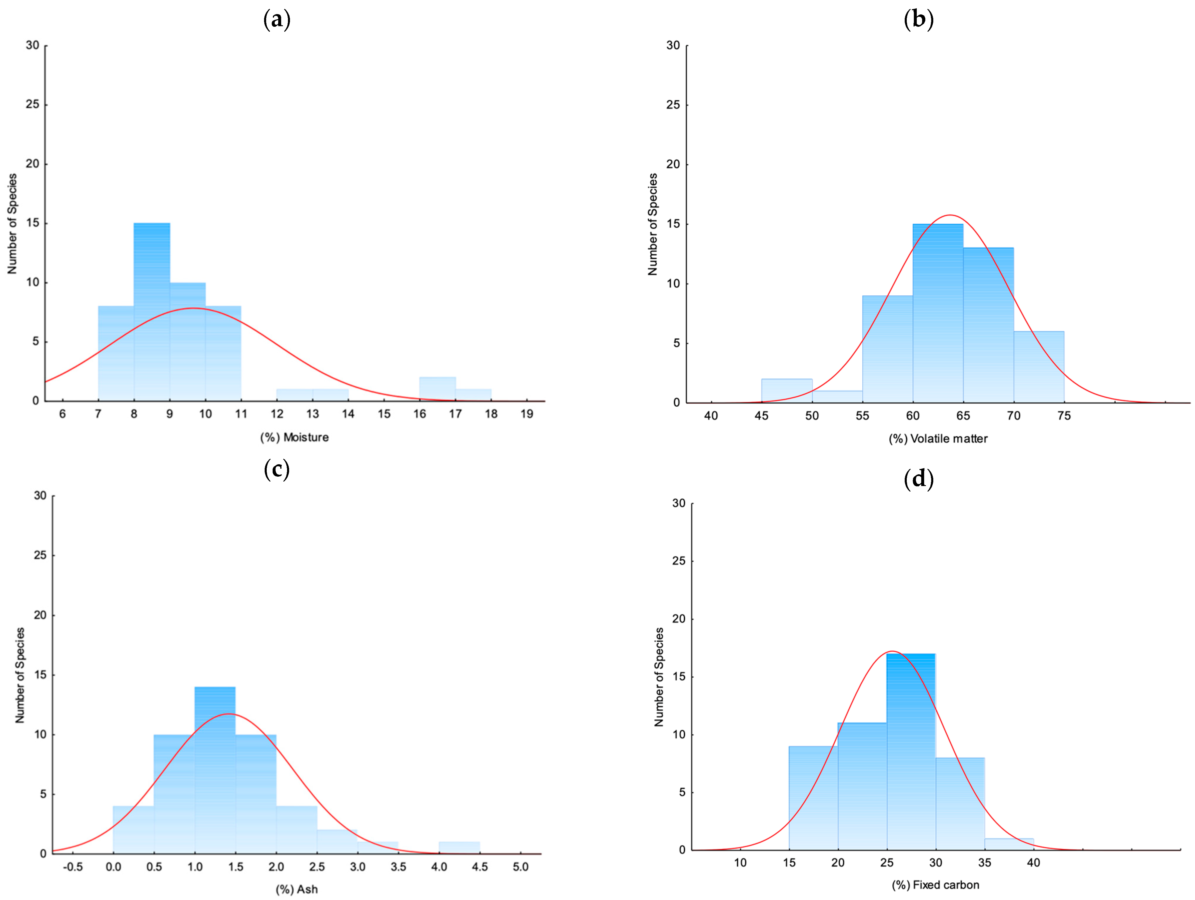
3.1.1. Proximate Analysis

The proximate analysis was conducted to assess the moisture, volatile matter, ash, and fixed carbon characteristics (

Table 1. Proximate analysis of analyzed species.

ID	Sample	Moisture ad ± σ (%)	Volatile Matter d ± σ (%)	Ash d ± σ (%)	Fixed Carbon d ± σ (%)
1	Abies alba	9.00 ± 0.300	61.50 ± 1.973	1.30 ± 0.027	28.20 ± 0.517
2	Abies grandis	8.30 ± 0.299	63.90 ± 0.717	0.90 ± 0.030	26.90 ± 0.534
3	Abies koreana	10.90 ± 0.185	59.70 ± 1.648	1.20 ± 0.033	28.20 ± 0.547
4	Abies nebrodensis	7.70 ± 0.367	64.70 ± 1.489	1.60 ± 0.065	26.00 ± 1.010
5	Abies nordmanniana	8.10 ± 0.188	70.00 ± 1.818	1.30 ± 0.066	20.60 ± 0.434
6	Abies pinsapo	9.20 ± 0.159	66.10 ± 0.662	2.00 ± 0.096	22.70 ± 0.448
7	Araucaria araucana	7.80 ± 0.394	59.10 ± 0.934	0.70 ± 0.023	32.40 ± 1.048
8	Calocedrus decurrens	10.90 ± 0.406	61.00 ± 0.807	3.40 ± 0.165	24.70 ± 0.524
9	Cedrus atlantica	10.20 ± 0.289	69.80 ± 0.882	1.50 ± 0.061	18.50 ± 0.328
10	Cedrus deodara	13.30 ± 0.471	59.70 ± 1.057	1.50 ± 0.064	25.50 ± 0.607
11	Cedrus libani	8.90 ± 0.255	55.80 ± 1.408	1.30 ± 0.039	34.00 ± 0.617
12	Chamaecyparis lawsoniana	7.10 ± 0.255	64.10 ± 1.089	1.60 ± 0.106	27.20 ± 0.692
13	Chamaecyparis obtusa	8.70 ± 0.464	71.70 ± 1.733	1.20 ± 0.031	18.40 ± 0.377
14	Cryptomeria japonica	9.20 ± 0.265	68.60 ± 2.156	1.80 ± 0.028	20.40 ± 0.306
15	Cupressus arizonica	8.60 ± 0.560	58.80 ± 1.033	1.20 ± 0.049	31.40 ± 1.126
16	Cupressus lusitanica	16.70 ± 0.460	66.90 ± 0.547	1.00 ± 0.052	15.40 ± 0.146
17	Cupressus macrocarpa	8.50 ± 0.253	71.00 ± 1.745	1.60 ± 0.058	18.90 ± 0.381
18	Cupressus sempervirens	8.40 ± 0.093	72.20 ± 1.430	1.40 ± 0.045	18.00 ± 0.508
19	Ginkgo biloba	17.00 ± 0.440	45.50 ± 1.469	4.10 ± 0.148	33.40 ± 0.990
20	Juniperus horizontalis	9.10 ± 0.177	70.10 ± 1.896	2.00 ± 0.078	18.80 ± 0.370
21	Juniperus oxycedrus	8.10 ± 0.201	68.60 ± 1.051	2.30 ± 0.121	21.00 ± 0.357
22	Juniperus sabina	7.70 ± 0.263	64.60 ± 0.881	2.60 ± 0.142	25.10 ± 0.395
23	Juniperus sabina var. tamariscifolia	9.50 ± 0.275	60.00 ± 1.473	2.30 ± 0.058	28.20 ± 0.606
24	Juniperus squamata	8.00 ± 0.184	66.20 ± 2.252	1.50 ± 0.043	24.30 ± 0.520
25	Larix decidua	10.60 ± 0.176	64.80 ± 2.081	1.60 ± 0.123	23.00 ± 0.500
26	Metasequoia glyptostroboides	10.20 ± 0.138	63.20 ± 1.989	1.40 ± 0.033	25.20 ± 1.042
27	Picea abies	9.20 ± 0.271	60.20 ± 0.790	2.50 ± 0.078	28.10 ± 0.627
28	Picea glauca	9.50 ± 0.108	68.60 ± 1.249	1.50 ± 0.053	20.40 ± 0.521
29	Picea pungens	8.30 ± 0.246	60.60 ± 2.057	1.90 ± 0.057	29.20 ± 0.655
30	Pinus heldreichii	10.70 ± 0.215	66.20 ± 1.733	1.30 ± 0.057	21.80 ± 0.661
31	Pinus mugo	7.50 ± 0.194	53.80 ± 0.612	0.80 ± 0.026	37.90 ± 0.683
32	Pinus nigra	9.00 ± 0.200	58.10 ± 1.255	0.10 ± 0.003	32.80 ± 0.526
33	Pinus pinaster	9.30 ± 0.677	58.00 ± 0.694	0.80 ± 0.031	31.90 ± 0.776
34	Pinus pinea	8.90 ± 0.306	65.10 ± 1.276	0.50 ± 0.023	25.50 ± 0.671
35	Pinus radiata	8.90 ± 0.433	63.00 ± 1.823	0.60 ± 0.041	27.50 ± 0.672
36	Pinus strobus	9.20 ± 0.329	71.10 ± 1.414	1.10 ± 0.034	18.60 ± 0.394
37	Pinus sylvestris	8.80 ± 0.197	60.70 ± 1.921	0.80 ± 0.020	29.70 ± 0.891
38	Podocarpus macrophyllus	17.40 ± 0.695	49.80 ± 1.784	2.30 ± 0.054	30.50 ± 0.616
39	Pseudotsuga menziesii	7.10 ± 0.125	63.90 ± 1.311	1.20 ± 0.054	27.80 ± 0.300
40	Sequoia sempervirens	9.60 ± 0.219	60.40 ± 0.580	0.60 ± 0.029	29.40 ± 0.783
41	Sequoiadendron giganteum	10.30 ± 0.315	56.50 ± 1.319	0.40 ± 0.016	32.80 ± 0.914
42	Taxodium distichum	8.30 ± 0.173	64.30 ± 1.844	1.10 ± 0.041	26.30 ± 0.831
43	Taxus baccata	12.40 ± 0.335	69.30 ± 0.951	1.30 ± 0.084	17.00 ± 0.345
44	Thuja plicata	10.20 ± 0.378	66.00 ± 1.216	0.80 ± 0.024	23.00 ± 0.854
45	Thujopsis dolobrata	7.90 ± 0.235	68.30 ± 1.882	0.20 ± 0.005	23.60 ± 0.377
46	Tsuga heterophylla	9.40 ± 0.229	70.80 ± 0.912	0.50 ± 0.021	19.30 ± 0.668

Note: _ad—air-dried basis; _d—dry basis.

). Moisture content in biomass significantly influences its energy efficiency; lower moisture content typically leads to higher energy output since less energy is required to evaporate water during combustion [26]. In this study, moisture content ranged from 7.10% to 17.40%. Species such as Pseudotsuga menziesii (39) and Chamaecyparis lawsoniana (12) exhibited the lowest moisture levels, indicating that they require minimal drying before combustion, making them more energy-efficient and cost-effective for bioenergy production. In contrast, Podocarpus macrophyllus (38) displayed the highest moisture content at 17.40%.

When comparing these results with the literature, similar studies often report moisture content in coniferous species ranging from 8% to 15% in air-dried samples [33,34]. The values observed in this study align with these findings, confirming that these species exhibit typical moisture levels for conifers. Lower moisture content, as observed in some species here, correlates with improved combustion performance, further supporting their potential as biofuels. Ferreira (2013) previously noted that moisture content in proximate analyses of coniferous species generally falls between 8% and 11% [35]. In this study, it was found that 71.74% of the species analyzed fell within this specified range (Figure 1).

Volatile matter plays a crucial role in determining the combustion behavior of biomass, with higher volatile content generally leading to more efficient energy release [36]. In this study, the volatile matter content ranged from 45.50% to 72.20%. Cupressus sempervirens (18) and Chamaecyparis obtusa (13) exhibited the highest volatile matter levels, indicating potentially superior combustion efficiency. Conversely, Ginkgo biloba (19) recorded the lowest value at 45.50%.

The literature often indicates that softwoods, including many coniferous species, typically have volatile matter content ranging between 65% and 75% [37]. The values observed in this study align with these expectations, suggesting that species like Cupressus sempervirens could be highly effective for energy production due to their elevated volatile matter content. However, according to Stanislav V. Vassilev (2010), volatile matter in biomass can vary widely, ranging from 48% to 86% [38]. In this study, 97.82% of the analyzed species fell within this range, with the exception of Ginkgo biloba (19), which had a lower volatile matter content at 45.50%. This reduced volatile matter in Ginkgo biloba may be attributed to its unique biochemical and physiological characteristics, potentially leading to a lower release of volatile substances during heating [39].

Ash content is a key indicator of the residue left after combustion. Lower ash content is preferable as it indicates fewer impurities and reduces the burden of ash disposal, making the biomass more desirable for energy applications [38]. In this study, ash content across the species ranged from 0.10% to 4.10%. Pinus nigra (32) and Thujopsis dolobrata (45) exhibited the lowest ash content, which is advantageous for bioenergy production as it minimizes post-combustion residue.

Ash content among the coniferous species varied from 0.2% to 2.20%, consistent with the findings of Khan (2009), who reported that ash content in biomass can range from 0.1% to 46% [40]. All the results in this study fall within this range, aligning with the existing literature. The low ash content in species like Pinus nigra (32) makes them particularly well suited for bioenergy production, as it matches the ideal properties highlighted in previous research.

Fixed carbon content, which is closely linked to the energy density of biomass, determines the amount of energy retained in the char after the volatile components are removed. In this study, fixed carbon content ranged from 15.40% to 37.90%. Pinus mugo (31) exhibited the highest fixed carbon content, indicating its potential for higher energy density and suitability for applications requiring long-lasting, slow-burning fuel. According to Stanislav V. Vassilev (2010), fixed carbon content in biomass can vary from 1% to 38% [38], and all species analyzed in our study fell within this specified range.

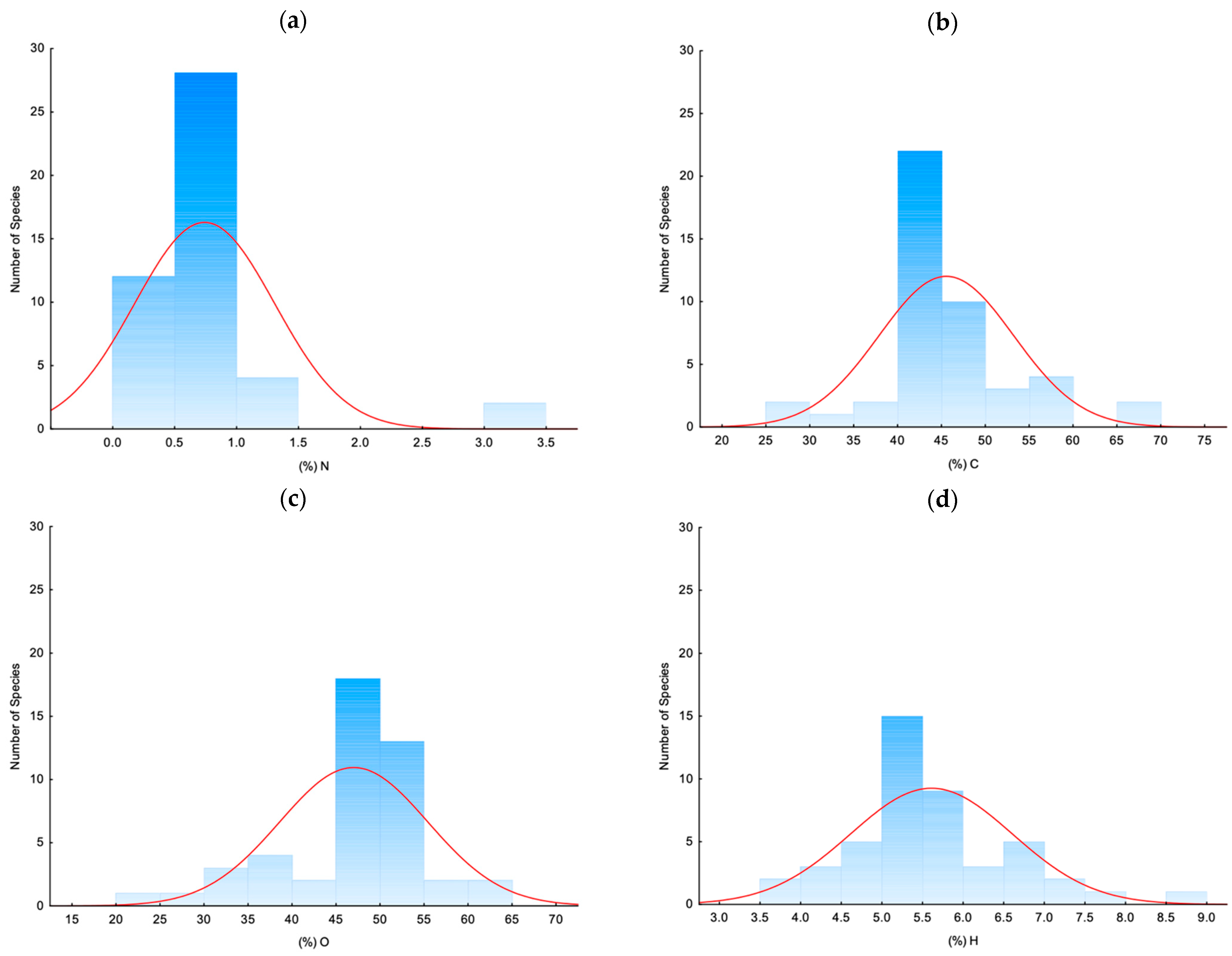
3.1.2. Elemental Chemical Analysis

The elemental composition of biomass is critical in assessing its potential for energy valorization. The analysis of the nitrogen (N), carbon (C), oxygen (O), and hydrogen (H) content across various species provides insights into their suitability for bioenergy production.

The analysis of nitrogen content across the studied coniferous species reveals that 86.96% of the species exhibit nitrogen levels below 1% (Figure 2). This finding is significant as it falls below the typical range of 1.0% to 12% [38]. The lower nitrogen content in these species is advantageous for bioenergy production because it implies reduced emissions of nitrogen oxides (NOx), which are harmful pollutants generated during combustion. This result aligns with the broader literature that emphasizes the environmental benefits of using low-nitrogen biomass in energy applications, particularly in reducing NOx emissions and associated environmental impacts [24].

Carbon is a key determinant of the energy content in biomass. Higher carbon content generally indicates greater energy potential, as carbon is the primary element that combusts to release energy. In this study, species such as Cedrus deodara (10), Sequoiadendron giganteum (41), and Taxodium distichum (42) demonstrated exceptionally high carbon content, with values of 63.84%, 77.92%, and 70.92%, respectively (

Table 2. Elemental analyses of analyzed species.

ID	Sample	Nd ± σ (%)	Cd ± σ (%)	Od ± σ (%)	Hd ± σ (%)
1	Abies alba	0.56 ± 0.015	47.04 ± 0.997	46.45 ± 0.824	4.64 ± 0.125
2	Abies grandis	1.45 ± 0.051	53.87 ± 0.894	38.42 ± 0.815	5.36 ± 0.264
3	Abies koreana	0.97 ± 0.037	57.94 ± 1.594	33.67 ± 0.770	6.21 ± 0.105
4	Abies nebrodensis	1.29 ± 0.097	46.09 ± 0.906	46.39 ± 1.175	4.63 ± 0.172
5	Abies nordmanniana	0.62 ± 0.022	49.83 ± 0.672	42.73 ± 0.926	5.51 ± 0.142
6	Abies pinsapo	1.13 ± 0.043	59.60 ± 1.802	31.11 ± 0.449	6.16 ± 0.362
7	Araucaria araucana	0.68 ± 0.024	44.77 ± 2.160	49.20 ± 0.857	4.65 ± 0.287
8	Calocedrus decurrens	0.68 ± 0.044	36.88 ± 0.829	55.89 ± 1.140	3.15 ± 0.138
9	Cedrus atlantica	0.84 ± 0.019	50.08 ± 1.210	42.51 ± 1.343	5.07 ± 0.155
10	Cedrus deodara	1.04 ± 0.031	63.84 ± 1.487	26.89 ± 0.649	6.73 ± 0.218
11	Cedrus libani	3.34 ± 0.107	47.72 ± 1.192	43.68 ± 0.840	3.95 ± 0.157
12	Chamaecyparis lawsoniana	0.62 ± 0.016	46.05 ± 0.548	47.03 ± 0.779	4.71 ± 0.104
13	Chamaecyparis obtusa	0.62 ± 0.028	51.12 ± 2.158	41.62 ± 0.730	5.43 ± 0.153
14	Cryptomeria japonica	0.54 ± 0.013	50.04 ± 1.390	42.48 ± 1.939	5.13 ± 0.118
15	Cupressus arizonica	0.52 ± 0.016	47.30 ± 1.281	46.03 ± 1.317	4.94 ± 0.213
16	Cupressus lusitanica	0.58 ± 0.034	50.23 ± 1.601	44.10 ± 0.691	4.10 ± 0.087
17	Cupressus macrocarpa	0.71 ± 0.029	48.37 ± 0.542	44.15 ± 1.036	5.17 ± 0.308
18	Cupressus sempervirens	0.42 ± 0.022	49.76 ± 2.136	43.29 ± 0.799	5.14 ± 0.138
19	Ginkgo biloba	0.77 ± 0.028	34.49 ± 0.758	58.29 ± 1.564	2.35 ± 0.126
20	Juniperus horizontalis	0.60 ± 0.019	49.77 ± 1.073	42.65 ± 1.799	4.97 ± 0.164
21	Juniperus oxycedrus	3.47 ± 0.067	48.21 ± 1.475	42.28 ± 0.906	3.74 ± 0.138
22	Juniperus sabina	0.60 ± 0.033	47.88 ± 1.084	44.25 ± 1.482	4.67 ± 0.126
23	Juniperus sabina var. tamariscifolia	0.69 ± 0.029	44.94 ± 0.760	47.24 ± 1.222	4.83 ± 0.129
24	Juniperus squamata	1.12 ± 0.056	48.86 ± 1.316	43.88 ± 1.164	4.65 ± 0.119
25	Larix decidua	0.22 ± 0.010	43.48 ± 0.666	50.92 ± 0.440	3.78 ± 0.111
26	Metasequoia glyptostroboides	0.32 ± 0.010	46.90 ± 0.893	46.70 ± 1.014	4.68 ± 0.223
27	Picea abies	0.84 ± 0.028	61.70 ± 1.590	28.81 ± 0.363	6.14 ± 0.139
28	Picea glauca	0.76 ± 0.032	50.34 ± 0.671	41.68 ± 0.793	5.71 ± 0.194
29	Picea pungens	0.75 ± 0.031	60.76 ± 1.045	29.91 ± 0.457	6.68 ± 0.194
30	Pinus heldreichii	0.59 ± 0.034	44.97 ± 1.201	48.67 ± 1.267	4.48 ± 0.095
31	Pinus mugo	0.66 ± 0.045	44.70 ± 0.869	49.65 ± 1.535	4.19 ± 0.102
32	Pinus nigra	0.55 ± 0.017	50.90 ± 1.179	43.32 ± 0.525	5.14 ± 0.225
33	Pinus pinaster	0.45 ± 0.011	46.25 ± 0.723	47.67 ± 0.683	4.83 ± 0.152
34	Pinus pinea	0.36 ± 0.013	40.53 ± 0.774	54.95 ± 1.333	3.66 ± 0.131
35	Pinus radiata	0.47 ± 0.009	46.92 ± 0.850	47.41 ± 0.652	4.60 ± 0.118
36	Pinus strobus	0.66 ± 0.056	53.08 ± 1.763	39.18 ± 1.155	5.98 ± 0.146
37	Pinus sylvestris	0.73 ± 0.017	60.94 ± 1.347	31.10 ± 0.740	6.43 ± 0.134
38	Podocarpus macrophyllus	1.01 ± 0.034	36.23 ± 0.997	58.30 ± 1.243	2.16 ± 0.062
39	Pseudotsuga menziesii	0.99 ± 0.030	45.50 ± 2.331	47.65 ± 0.961	4.66 ± 0.164
40	Sequoia sempervirens	0.32 ± 0.009	45.85 ± 0.502	49.00 ± 1.487	4.23 ± 0.124
41	Sequoiadendron giganteum	0.75 ± 0.023	77.92 ± 1.314	12.74 ± 0.159	8.20 ± 0.277
42	Taxodium distichum	0.76 ± 0.050	70.92 ± 1.340	20.01 ± 0.242	7.21 ± 0.230
43	Taxus baccata	0.63 ± 0.034	49.99 ± 1.305	43.45 ± 1.643	4.63 ± 0.199
44	Thuja plicata	0.27 ± 0.011	60.65 ± 0.846	31.89 ± 1.103	6.39 ± 0.214
45	Thujopsis dolobrata	0.81 ± 0.035	45.93 ± 1.431	49.00 ± 1.608	4.06 ± 0.213
46	Tsuga heterophylla	0.64 ± 0.018	51.68 ± 1.305	41.43 ± 0.785	5.75 ± 0.104

). These species are particularly promising for energy valorization due to their high carbon content, which suggests a higher calorific value and better efficiency in energy production. The carbon content of the analyzed species shows that 56.52% of them fall within the 40–50% range, while 26.08% have carbon contents below 42%. This distribution is slightly lower than the typical carbon content range of 42% to 71% [38]. Carbon content is a critical determinant of biomass energy potential, with higher carbon percentages generally correlating with higher calorific values. The relatively lower carbon content in a portion of the species suggests that these species may yield lower energy outputs upon combustion compared to species with higher carbon content. This observation is consistent with studies that link higher carbon content to increased energy potential in biomass, highlighting the importance of selecting species with optimal carbon levels for efficient bioenergy production [41,42].

Oxygen content inversely affects the energy value of biomass; higher oxygen levels typically correlate with lower energy density. Species like Sequoiadendron giganteum (41) and Taxodium distichum (42) not only have high carbon content but also relatively low oxygen content at 12.74% and 20.01%, respectively. This combination enhances their energy density, making them more efficient as biofuels. In contrast, species such as Podocarpus macrophyllus (38) and Ginkgo biloba (19) have higher oxygen contents of 58.30% and 58.29%, respectively. This high oxygen content may dilute the energy content per unit mass, leading to less efficient combustion. Therefore, these species might be less suitable for direct combustion applications but could be considered for other forms of energy conversion, such as gasification, where oxygen content plays a different role [42,43].

Hydrogen also contributes to the heating value of biomass, although to a lesser extent than carbon. Higher hydrogen content can improve combustion efficiency. Cedrus deodara (10), Sequoiadendron giganteum (41), and Taxodium distichum (42) again stand out with hydrogen contents of 6.73%, 8.20%, and 7.21%, respectively, further reinforcing their suitability for energy production. On the other hand, species like Ginkgo biloba (19) and Podocarpus macrophyllus (38) have lower hydrogen content at 2.35% and 2.16%, respectively. The lower hydrogen content, combined with high oxygen content, may contribute to less efficient energy release during combustion, aligning with their overall lower energy potential [41]. The hydrogen content in the analyzed species predominantly falls within the 5% to 7% range, with 69.57% of the species within this bracket. This is well within the typical range of 3% to 11% [38,41,43].

3.1.3. Calorimetric Analysis

The calorimetric analysis revealed notable variations in the gross heating value (GHV) among the studied species, as shown in

Table 3. GHV and NHV of studied coniferous species.

ID	Sample	GHVd ± σ (MJ/kg)	NHVd ± σ (MJ/kg)
1	Abies alba	18.39 ± 0.690	17.43 ± 0.646
2	Abies grandis	18.48 ± 0.621	17.38 ± 0.652
3	Abies koreana	18.17 ± 0.487	16.89 ± 0.495
4	Abies nebrodensis	18.34 ± 0.345	17.39 ± 0.364
5	Abies nordmanniana	18.76 ± 0.894	17.62 ± 0.878
6	Abies pinsapo	18.46 ± 0.539	17.19 ± 0.551
7	Araucaria araucana	18.23 ± 0.714	17.27 ± 0.714
8	Calocedrus decurrens	14.39 ± 0.618	13.74 ± 0.626
9	Cedrus atlantica	18.02 ± 0.546	16.98 ± 0.575
10	Cedrus deodara	17.55 ± 0.653	16.16 ± 0.637
11	Cedrus libani	17.70 ± 0.419	16.89 ± 0.411
12	Chamaecyparis lawsoniana	18.26 ± 1.109	17.29 ± 1.116
13	Chamaecyparis obtusa	18.54 ± 0.761	17.42 ± 0.750
14	Cryptomeria japonica	18.31 ± 0.419	17.25 ± 0.429
15	Cupressus arizonica	18.04 ± 0.677	17.02 ± 0.692
16	Cupressus lusitanica	16.75 ± 0.394	15.91 ± 0.421
17	Cupressus macrocarpa	18.23 ± 0.970	17.16 ± 0.960
18	Cupressus sempervirens	18.24 ± 0.528	17.18 ± 0.530
19	Ginkgo biloba	13.45 ± 0.458	12.97 ± 0.454
20	Juniperus horizontalis	18.10 ± 0.687	17.08 ± 0.676
21	Juniperus oxycedrus	17.61 ± 0.495	16.84 ± 0.480
22	Juniperus sabina	18.03 ± 0.641	17.07 ± 0.637
23	Juniperus sabina var, tamariscifolia	17.72 ± 0.814	16.73 ± 0.813
24	Juniperus squamata	18.10 ± 0.347	17.14 ± 0.369
25	Larix decidua	16.53 ± 0.463	15.75 ± 0.451
26	Metasequoia glyptostroboides	18.14 ± 0.524	17.18 ± 0.539
27	Picea abies	18.33 ± 0.386	17.07 ± 0.362
28	Picea glauca	18.63 ± 0.718	17.45 ± 0.738
29	Picea pungens	18.24 ± 0.813	16.86 ± 0.813
30	Pinus heldreichii	17.26 ± 0.916	16.34 ± 0.922
31	Pinus mugo	18.62 ± 0.446	17.76 ± 0.469
32	Pinus nigra	18.76 ± 0.636	17.70 ± 0.621
33	Pinus pinaster	18.60 ± 0.658	17.61 ± 0.607
34	Pinus pinea	18.52 ± 0.732	17.77 ± 0.732
35	Pinus radiata	18.39 ± 0.764	17.44 ± 0.748
36	Pinus strobus	19.19 ± 0.664	17.96 ± 0.635
37	Pinus sylvestris	18.33 ± 0.747	17.01 ± 0.750
38	Podocarpus macrophyllus	13.21 ± 0.486	12.77 ± 0.481
39	Pseudotsuga menziesii	18.24 ± 0.342	17.28 ± 0.360
40	Sequoia sempervirens	18.29 ± 1.386	17.42 ± 1.418
41	Sequoiadendron giganteum	18.78 ± 1.413	17.09 ± 1.429
42	Taxodium distichum	18.22 ± 0.962	16.73 ± 0.938
43	Taxus baccata	17.38 ± 0.444	16.43 ± 0.428
44	Thuja plicata	18.36 ± 1.405	17.04 ± 1.432
45	Thujopsis dolobrata	18.32 ± 0.822	17.48 ± 0.799
46	Tsuga heterophylla	18.48 ± 0.712	17.30 ± 0.712

.

Podocarpus macrophyllus (38) recorded the lowest GHV at 13.21 MJ/kg, along with the lowest net heating value (NHV) at 12.77 MJ/kg. In contrast, Pinus strobus (36) exhibited the highest GHV at 19.19 MJ/kg, which also corresponded to the highest NHV at 17.96 MJ/kg.

Figure 3 illustrates the distribution of the gross heating value (GHV) for the coniferous species studied. The analysis shows that 76.09% of the samples had a GHV greater than 18 MJ/kg, indicating a strong potential for energy production in these species. Figure 4 presents the distribution of the net heating value (NHV), revealing that 50% of the samples were concentrated within the 15 to 17 MJ/kg range. This suggests that, while the initial energy content (GHV) is high, the actual usable energy (NHV), accounting for losses such as moisture content, is slightly lower but still within an effective range for bioenergy applications [44], aligning with findings in the literature [43].

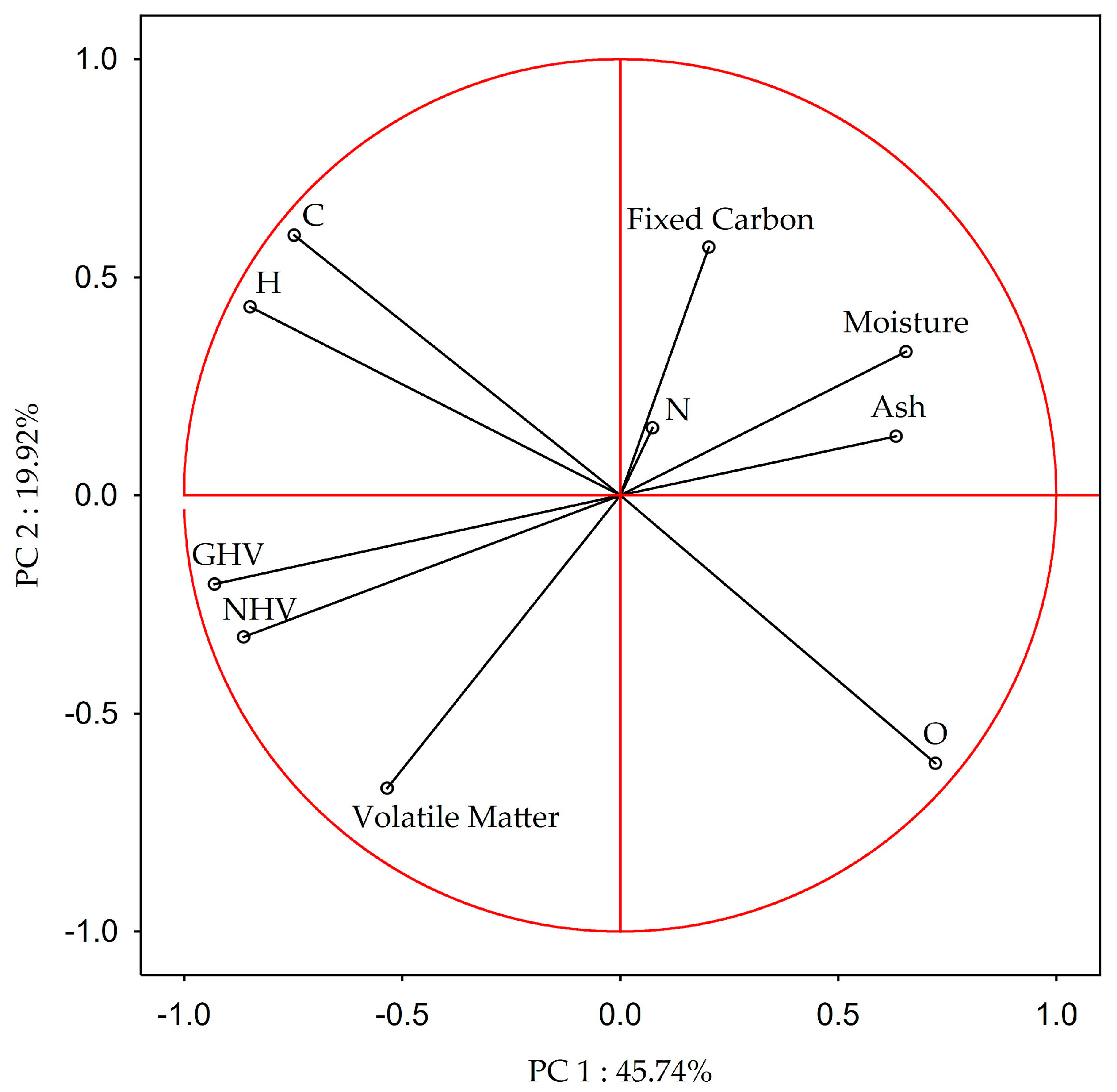
3.2. Relationship between Proximate Analysis, Elemental Composition, and Heating Values of Biomass

In this study, principal component analysis (PCA) served as an unsupervised exploratory technique to examine the presence of discrepant samples and identify patterns in the distribution of samples based on their energy potential. Furthermore, PCA was utilized to explore relationships between variables and potential clusters. The analysis comprehended results from proximate analysis, elemental analysis, and calorimetric analysis. From the obtained results, it was observed that PCA yielded three principal components (PCs) explaining 81.59% of the total variation in the original dataset (Figure 5).

PC1, which explains 45.74% of the total original variance, correlates positively with the oxygen content of the species and negatively with the carbon, hydrogen, GHV, and NHV content. PC2, which explains 19.92% of the original total variance, correlates negatively with fixed carbon. In PC3, which explains 16.13% of the original total variability, none of the variables studied was decisive. These data demonstrate, as expected, a positive correlation between the NHV and GHV and the carbon and hydrogen content of the species studied. Conversely, there is a negative correlation with the oxygen content.

However, since the PCs are orthogonal, meaning they are not correlated, the relationship of the fixed carbon content with PC2 suggests, as anticipated, that GHV and NHV are not directly related to this variable. Conversely, the fixed carbon content exhibits a weak association with the elemental composition of these samples, as shown in Figure 6.

In Figure 7, we can see that most species are clustered close to the origin. However, there are species with discrepant behavior, such as the species Ginkgo biloba (19), Podocarpus macrophyllus (38), and Calocedrus decurrens (8), which have a positive PC1 value, while the species Taxodium distichum (42) and Sequoiadendron giganteum (41) have a negative PC1 value.

On the other hand, the species Ginkgo biloba (19), Podocarpus macrophyllus (38), and Calocedrus decurrens (8) have the highest oxygen contents and the lowest carbon and hydrogen contents and, consequently, also have the lowest GHV and NHV, unlike the species Taxodium distichum (42) and Sequoiadendron giganteum (41), which have the highest carbon and hydrogen contents and, therefore, the highest contents.

Cluster analysis was performed on the PC1 and PC2 scores to evaluate the similarities between the different species. This was conducted using Euclidean distance and Ward’s hierarchical agglomerative method [45].

As shown in Figure 8, seven distinct clusters were formed, with a cut-off of 6 based on the linkage distances displayed in Figure 9. Each cluster represents a group of species with similar chemical profiles and energy characteristics.

Cluster 1 (Species 38, 19, and 8) comprises species that exhibit closely related properties, particularly in terms of moisture content and fixed carbon levels. These species are characterized by their potential for efficient energy production, making them favorable candidates for bioenergy applications where consistent combustion and energy release are required. The species in cluster 2 (Species 42, 41, 29, 27, 6, 10, 44, 37, and 3) are grouped due to their similar volatile matter content and ash composition, indicating comparable combustion characteristics. These species are likely to perform similarly in bioenergy processes, providing steady energy output and possibly requiring similar processing conditions.

Species in cluster 3 (Species 30, 25, 43, and 16) share a higher fixed carbon content, which is crucial for sustained energy release during combustion. Their clustering suggests that they are particularly well suited for applications where high energy density and prolonged combustion are desired. Cluster 4 (Species 18, 17, 20, 14, 9, 46, 36, 28, 13, and 5) includes species with similar volatile matter and moisture content, which are essential for efficient ignition and combustion. These species are likely to be versatile in various bioenergy processes, offering flexibility in their use for energy production. The two species in cluster 5 (Species 21 and 11) are grouped together because of their similarity on elemental composition and NHV value. Species in cluster 6 (Species 23, 22, 39, 12, 24, 4, and 2) share characteristics that suggest a balanced composition of moisture, volatile matter, and fixed carbon. This balance makes them reliable for consistent energy output and may require minimal preprocessing, making them efficient choices for bioenergy use. Finally, cluster 7 (Species 45, 34, 32, 31, 40, 35, 26, 33, 7, 15, and 1) groups species with high moisture content and relatively high volatile matter. These species are likely to require drying or other preprocessing steps before being used for energy production but could offer substantial energy output once processed.

To understand the relative contribution of the chemical composition of the species to the NHV value, a multiple regression analysis was carried out using the values from the elemental chemical analysis, the nitrogen, carbon, oxygen, hydrogen, and sulfur contents, and values obtained from the proximate analysis, moisture, ash, fixed carbon, and volatile matter. The “best subset” method was used to build the MLR models using R² _Adjusted. The multicollinearity of the predictive variables was determined using the “Variable Inflation Factor” and tolerance, and no problems were detected.

The estimation of the parameters for all the models was assessed using the Student’s t-test (p < 0.05). The model obtained was statistically significant (R = 0.906; F = 64.14; p < 0.001), making it possible to account for 82% of the variance observed in the NHV values (R² = 0.820; R² _Adjusted = 0.808).

Moisture content had the greatest weight in the model, followed by ash content and hydrogen content. Moisture content had the highest beta value, showing that it is the variable with the greatest contribution to the regression equation, keeping the other variables constant.

Its zero-order regression coefficient (r = −0.787) shows that this variable shares a large portion of its variability with NHV (62%), followed by ash content (r = −0.668; 45%) and, finally, hydrogen content (r = 0.513; 26%).

The value of the square of the structural correlation coefficient (rX,y) shows that the moisture content shares the largest portion of its variance (rX,y = −0.870; 76%) with the predicted NHV values, followed by the ash content (rX,y = −0.738; 54%) and the hydrogen content (rX,y = 0.566; 32%).

The product between beta × r allows us to calculate the partitioning of the regression effect into nonoverlapping parts based on the interaction of the beta coefficients and the zero-order correlation coefficients with the dependent variable [46], showing that, in this respect, the moisture content (47%) and the ash content (27%) are responsible for most of the variation in the regression equation, followed by the hydrogen content with 9%.These results clearly show that, for the coniferous species studied, the variation in NHV is mostly explained by the variation in moisture content and ash content and, to a lesser extent, by hydrogen content (Figure 10).

4. Conclusions

This study provides a detailed analysis of the thermo-chemical properties of various coniferous species, highlighting their diverse energy potentials. Key factors such as moisture content, ash content, and hydrogen content emerged as significant determinants of the net heating value (NHV), with species like Pinus pinea and Sequoiadendron giganteum identified as particularly promising for bioenergy production due to their high energy density and combustion efficiency. The results have immediate applications in developing predictive models to estimate energy yields and optimize biomass blending strategies. Additionally, the findings can guide the design of tailored combustion systems and inform sustainable forest management practices that prioritize species with the highest energy potential.

Future research should focus on developing advanced predictive models using machine learning, exploring the energy potential of less common coniferous species, and conducting longitudinal studies on the impact of biomass aging. Moreover, integrating molecular-level analysis and conducting life cycle assessments (LCA) will provide a more comprehensive understanding of the environmental and economic impacts of using coniferous biomass for energy.

Overall, this study lays the groundwork for more efficient and sustainable utilization of coniferous biomass as a renewable energy source, contributing to the global transition away from fossil fuels.

References

1. Adebayo, T.S.; Awosusi, A.A.; Kirikkaleli, D.; Akinsola, G.D.; Mwamba, M.N. Can CO2 emissions and energy consumption determine the economic performance of South Korea? A time series analysis. Environ. Sci. Pollut. Res. 2021, 28, 38969–38984. [Google Scholar] [CrossRef]
2. Yuping, L.; Ramzan, M.; Xincheng, L.; Murshed, M.; Awosusi, A.A.; Bahs, I.; Adebayo, T.S. Determinants of carbon emissions in Argentina: The roles of renewable energy consumption and globalization. Energy Rep. 2021, 7, 4747–4760. [Google Scholar] [CrossRef]
3. Maluf, C.D. Qual a Importância da Energia Renovável. AmbScience Engenharia. Available online: https://ambscience.com/energia-renovavel/ (accessed on 3 May 2022).
4. European Environment Agency. About Energy, EEA 2018. Available online: https://www.eea.europa.eu/pt/themes/energy/about-energy (accessed on 3 May 2022).
5. Awosusi, A.A.; Adebayo, T.S.; Altuntaş, M.; Agyekum, E.B.; Zawbaa, H.M.; Kamel, S. The dynamic impact of biomass and natural resources on ecological footprint in BRICS economies: A quantile regression evidence. Energy Rep. 2022, 8, 1979–1994. [Google Scholar] [CrossRef]
6. Júnior, S.V.; Soares, I.P. Chemical analysis of biomass—A review of techniques and applications. Quím. Nova 2014, 37, 709–715. [Google Scholar] [CrossRef]
7. DGEG. Fontes de Energia Renovável: Biomassa Assegura 45% da Produção. Energia 2021. Available online: https://florestas.pt/valorizar/energia-renovavel-biomassa-assegura-56-da-producao/#:~:text=A%20produ%C3%A7%C3%A3o%20anual%20de%20energia,Energia%20e%20Geologia%20(DGEG) (accessed on 31 May 2022).
8. Baker, J.S.; Wade, C.M.; Sohngen, B.L.; Ohrel, S.; Fawcett, A.A. Potential complementarity between forest carbon sequestration incentives and biomass energy expansion. Energy Policy 2019, 126, 391–401. [Google Scholar] [CrossRef]
9. ICNF. IFN6—6° Inventário Florestal Nacional—Relatório Final; Instituto da Conservação da Natureza e das Florestas: Lisbon, Portugal, 2015. [Google Scholar]
10. Röser, D.; Asikainen, A.; Stupak, I.; Pasanen, K. Forest Energy Resources and Potentials. In Sustainable Use of Forest Biomass for Energy; Röser, D., Asikainen, A., Raulund-Rasmussen, K., Stupak, I., Eds.; Managing Forest Ecosystems; Springer: Dordrecht, The Netherlands, 2008; Volume 12. [Google Scholar] [CrossRef]
11. Instituto Nacional de Estatística Statistics Portugal. Contas Económicas da Silvicultura. Available online: https://www.ine.pt/xportal/xmain?xpid=INE&xpgid=ine_destaques&DESTAQUESdest_boui=473108475&DESTAQUESmodo=2 (accessed on 31 May 2022).
12. Girón, R.P.; Ruiz, B.; Fuente, E.; Gil, R.R.; Suárez-Ruiz, I. Properties of fly ash from forest biomass combustion. Fuel 2013, 114, 71–77. [Google Scholar] [CrossRef]
13. Ravindranath, N.H.; Hall, D.O. Biomass, Energy, and Environment: A Developing Country Perspective from India; Oxford Academic: Oxford, UK, 1995. [Google Scholar] [CrossRef]
14. Demirbas, A. Combustion characteristics of different biomass fuels. Prog. Energy Combust. Sci. 2004, 30, 219–230. [Google Scholar] [CrossRef]
15. Hiloidhari, M.; Baruah, D.C.; Kumaria, M.; Kumari, S.; Thakur, I.S. Prospect and potential of biomass power to mitigate climate change: A case study in India. J. Clean. Prod. 2019, 220, 931–944. [Google Scholar] [CrossRef]
16. Sulaiman, C.; Abdul-Rahim, A.S.; Ofozor, C.A. Does wood biomass energy use reduce CO2 emissions in European Union member countries? Evidence from 27 members. J. Clean. Prod. 2020, 253, 119996. [Google Scholar] [CrossRef]
17. IRENA. Global Energy Transformation: A Roadmap to 2050 (2019 Edition); International Renewable Energy Agency: Abu Dhabi, United Arab Emirates, 2019. [Google Scholar]
18. Observatório da Energia; DGEG—Direção Geral de Energia e Geologia; Direção de Serviços de Planeamento Energético e Estatística; ADENE—Agência para a Energia; Unidade de Informação. Energia em Números; ADENE: Lisbon, Portugal, 2020. [Google Scholar]
19. Hall, D.O.; Rosillo-Calle, F.; de Groot, P. Biomass energy: Lessons from case studies in developing countries. Energy Policy 1992, 20, 62–73. [Google Scholar] [CrossRef]
20. García, R.; Pizarro, C.; Lavín, A.G.; Bueno, J.L. Characterization of Spanish biomass wastes for energy use. Bioresour. Technol. 2012, 103, 249–258. [Google Scholar] [CrossRef]
21. McKendry, P. Energy production from biomass (part 1): Overview of biomass. Bioresour. Technol. 2002, 83, 37–46. [Google Scholar] [CrossRef]
22. Vassilev, S.V.; Vassileva, C.G.; Vassilev, V.S. Advantages and disadvantages of composition and properties of biomass in comparison with coal: An overview. Fuel 2015, 158, 330–350. [Google Scholar] [CrossRef]
23. ISO 18135:2017 (E); Solid Biofuels—Sampling. ISO: Geneva, Switzerland, 2017.
24. Makepa, D.C.; Chihobo, C.H. Sustainable pathways for biomass production and utilization in carbon capture and storage—A review. Biomass Convert. Biorefinery 2024. [Google Scholar] [CrossRef]
25. Sorek, N.; Yeats, T.H.; Szemenyei, H.; Youngs, H.; Somerville, C.R. The Implications of Lignocellulosic Biomass Chemical Composition for the Production of Advanced Biofuels. BioScience 2014, 64, 192–201. [Google Scholar] [CrossRef]
26. Michael, T.; Dananjali, G.; Naoki, H.; Anke, M.; Saman, S. Effects of Elevated Carbon Dioxide on Photosynthesis and Carbon Partitioning: A Perspective on Root Sugar Sensing and Hormonal Crosstalk. Front. Physiol. 2017, 8, 578. [Google Scholar] [CrossRef]
27. ISO 14780:2017 (E); Solid Biofuels—Solid Biofuels—Sample Preparation. ISO: Geneva, Switzerland, 2017.
28. ISO 18134-3:2015 (E); Solid Biofuels—Determination of Moisture Content Oven Dry Method. ISO: Geneva, Switzerland, 2015.
29. ISO 18122:2015 (E); Solid Biofuels—Determination of Ash Content, Geneva. ISO: Geneva, Switzerland, 2015.
30. ISO 18123:2015 (E); Solid Biofuels—Determination of the Content of Volatile Matter. ISO: Geneva, Switzerland, 2015.
31. ISO 16948:2015 (E); Solid Biofuels—Determination of Total Content of Carbon, Hydrogen and Nitrogen. ISO: Geneva, Switzerland, 2015.
32. ISO 18125:2017 (E); Solid Biofuels—Determination of Calorific Value. ISO: Geneva, Switzerland, 2017.
33. Hartmann, H. Solid Biofuels, Fuels, and Their Characteristics. In Encyclopedia of Sustainability Science and Technology; Meyers, R., Ed.; Springer: New York, NY, USA, 2017. [Google Scholar] [CrossRef]
34. Shojaeiarani, J.; Bajwa, D.S.; Bajwa, S.G. Properties of densified solid biofuels in relation to chemical composition, moisture content, and bulk density of the biomass. BioResources 2019, 14, 4996–5015. [Google Scholar] [CrossRef]
35. Ferreira, A.C.O. Caracterização de Vários Tipos de Biomassa para Valorização Energética. Master’s Thesis, Universidade de Aveiro, Departamento de Engenharia Mecânica, Aveiro, Portugal, 2013. [Google Scholar]
36. Vilas-Boas, A.C.M.; Tarelho, L.A.C.; Oliveira, H.S.M.; Silva, F.G.C.S.; Pio, D.T.; Matos, M.A.A. Valorisation of residual biomass by pyrolysis: Influence of process conditions on products. Sustain. Energy Fuels 2024, 8, 379–396. [Google Scholar] [CrossRef]
37. Chen, L.; Lin, S.; Liang, J.; Evrendilek, F.; He, Y.; Liu, J. Combustion behaviors of Lycium barbarum L.: Kinetics, thermodynamics, gas emissions, and optimization. Biomass Convers. Biorefinery 2024. [Google Scholar] [CrossRef]
38. Vassilev, S.; Baxter, D.; Andersen, L.; Vassileva, C. An Overview of the Chemical Composition of Biomass. Fuel 2010, 89, 913–933. [Google Scholar] [CrossRef]
39. Chang, B.; Ma, K.; Lu, Z.; Lu, J.; Cui, J.; Wang, L.; Jin, B. Physiological, Transcriptomic, and Metabolic Responses of Ginkgo biloba L. to Drought, Salt, and Heat Stresses. Biomolecules 2020, 10, 1635. [Google Scholar] [CrossRef] [PubMed]
40. Khan, A.A.; de Jong, W.; Jansens, P.J.; Spliethoff, H. Biomass combustion in fluidized bed boilers: Potential problems and remedies. Fuel Process. Technol. 2009, 90, 21–50. [Google Scholar] [CrossRef]
41. Ali, F.; Dawood, A.; Hussain, A.; Alnasir, M.H.; Khan, M.A.; Butt, T.M.; Janjua, N.K.; Hamid, A. Fueling the future: Biomass applications for green and sustainable energy. Discov. Sustain. 2024, 5, 156. [Google Scholar] [CrossRef]
42. Varghese, R.T.; Antony, T.; Chirayil, C.J. Biomass: Abundance, Classification, Energy Potential. In Handbook of Advanced Biomass Materials for Environmental Remediation; Thomas, S., Chirayil, C.J., Varghese, R.T., Eds.; Materials Horizons: From Nature to Nanomaterials; Springer: Singapore, 2024. [Google Scholar] [CrossRef]
43. Matin, B.; Leto, J.; Antonović, A.; Brandić, I.; Jurišić, V.; Matin, A.; Krička, T.; Grubor, M.; Kontek, M.; Bilandžija, N. Energetic Properties and Biomass Productivity of Switchgrass (Panicum virgatum L.) under Agroecological Conditions in Northwestern Croatia. Agronomy 2023, 13, 1161. [Google Scholar] [CrossRef]
44. Petráš, R.; Mecko, J.; Kukla, J.; Kuklová, M.; Krupová, D.; Pástor, M.; Raček, M.; Pivková, I. Energy Stored in Above-Ground Biomass Fractions and Model Trees of the Main Coniferous Woody Plants. Sustainability 2021, 13, 12686. [Google Scholar] [CrossRef]
45. Ward, J.H. Hierarchical grouping to optimize an objective function. J. Am. Stat. Assoc. 1963, 58, 236–244. [Google Scholar] [CrossRef]
46. Nathans, L.; Oswald, F.; Nimon, K. Interpreting multiple linear regression: A guidebook of variable importance. Practical Assessment. Res. Eval. 2012, 17, 1–19. [Google Scholar] [CrossRef]
Figure 1. Distribution of proximate analysis results. (a) Distribution of species by moisture content (%), (b) distribution of species by volatile matter content (%), (c) distribution of species by ash content (%), and (d) distribution of species by fixed carbon content (%).
Sustainability 16 07622 g001
Figure 2. Distribution of elemental chemical analysis results. (a) Distribution of species by nitrogen content (%), (b) distribution of species by carbon content (%), (c) distribution of species by oxygen content (%), and (d) distribution of species by hydrogen content (%).
Sustainability 16 07622 g002
Figure 3. Distribution of GHV of studied coniferous species.
Sustainability 16 07622 g003
Figure 4. Distribution of NHV of studied coniferous species.
Sustainability 16 07622 g004
Figure 5. Eigenvalues of correlation matrix.
Sustainability 16 07622 g005
Figure 6. Projection of the variables onto the factor plane (1 × 2).
Sustainability 16 07622 g006
Figure 7. Projection of species on the (1 × 2) plane.
Sustainability 16 07622 g007
Figure 8. Tree diagram for the studied species.
Sustainability 16 07622 g008
Figure 9. Plot of linkage distances across steps.
Sustainability 16 07622 g009
Figure 10. Pareto chart of t-values for coefficients.
Sustainability 16 07622 g010