The Relationship Between Three-Dimensional Spatial Structure and CO₂ Emission of Urban Agglomerations Based on CNN-RF Modeling: A Case Study in East China

Abstract

Good urban design helps mitigate carbon dioxide emissions and is important for achieving global low-carbon goals. Previous studies have mostly focused on the two-dimensional level of urban socio-economic activities, urban land use changes, and urban morphology, neglecting the importance of the three-dimensional spatial structure of cities. This study takes 30 cities in East China as an example. By using urban building data and carbon emission datasets, four machine learning algorithms, BP, RF, CNN, and CNN-RF, are established to build a CO₂ emission prediction model based on three-dimensional spatial structure, and the main influencing factors are further studied. The results show that the CNN-RF model performed optimally in both the testing and validation phases, with the coefficient of determination (R²), root mean square error (RMSE), and residual prediction deviation (RPD) of 0.85, 0.82; 10.60, 22.32; and 2.53, 1.92, respectively. Meanwhile, in the study unit, S, V, NHB, AN, BCR, SCD, and FAR have a greater impact on CO₂ emissions. This indicates a strong correlation between urban three-dimensional spatial structure and carbon emissions. The CNN-RF model can effectively evaluate the relationship between them, providing strategic support for spatial optimization of low-carbon cities.

1. Introduction

In recent years, as a result of accelerated urbanization, much attention has been paid to the relationship between greenhouse gas emissions and the urbanization process. The large amount of greenhouse gas emissions has led to a series of environmental issues, such as global warming and rising sea levels [1,2]. Cities, as the largest places of consumption and activity, account for about 70 percent of global greenhouse gas emissions. Reducing urban CO₂ emissions is of great significance in alleviating global environmental problems [3].

Current research on urban carbon emissions covers several areas [4], such as changes in policy regimes [5,6], population changes [7,8], transportation organizations [9,10], etc. Given the strong correlation between carbon emissions and urban development, existing studies have focused more on how economic and social factors affect carbon emission levels [11]. For example, Shahbaz et al. used bootstrap boundary tests to explore the effects of economic growth [12], and Hailemariam et al. used the environmental Kuznets curve to reveal the nonlinear relationship between economic growth and CO₂ emissions and found that a high-income gap will produce more CO₂ emissions. They found that financial development and energy consumption have a major effect on carbon dioxide emissions over different periods, concluding that financial development and R&D expenditures are key tools for achieving carbon reduction targets [13]. However, these studies mainly focused on intra-city activities and lacked consideration of carbon reduction in the city itself. Due to this, a large number of scholars have begun to notice the link between urban spatial structure and carbon emissions, and many studies have shown that the role of urban spatial structure in carbon emission reduction should not be underestimated [14].

The spatial structure of the urban environment is divided into two and three dimensions, but current research focuses mainly on the two-dimensional level. Urban sprawl is considered to be the main reason for the increase in carbon emissions [15,16], and methods such as the development of baseline regression models, autoregressive distribution lag (ARDL) methods, environmental Kuznets curves, and machine learning have been applied to the study. For example, Wu et al. developed a model of urban sprawl based on the quantification of remotely sensed nighttime lighting data, which demonstrated that urban sprawl increases carbon emissions by a large amount [17]. Sufyanullah et al. found a correlation ratio between urban sprawl and increased CO₂ emissions, in that an increase of 1% in the urban area is associated with a 0.901% increase in carbon emissions [18]. Furthermore, Hanif looked at energy consumption and showed that urban sprawl leading to high energy demand will increase carbon emissions [19]. Ding et al. used a hybrid model to project land use change in 2035 to simulate changes in carbon emissions [20]. Xia et al. constructed four scenarios of the development of Hangzhou in 2035 based on different modes of urban growth and land use structures, showing that rational land use management has a greater potential to reduce carbon emissions in the urbanization process [21]. The relationship between urban land use change and functional urban areas and CO₂ emissions has also received attention [22,23,24]. In addition to these studies, Falahatkar et al. used panel data to analyse the relationship between urban form and carbon dioxide emissions, showing that an increase in the urban area and a decrease in urban compactness leads to high carbon emissions [25]. This is supported by the study of Cucchiella et al. who concluded that compact development can effectively reduce carbon emissions [26]. These studies are highly instructive for the planning of low-carbon cities but are mostly biased toward the horizontal structure of cities.

In fact, in addition to the two-dimensional dimension, the three-dimensional spatial structure of cities is also closely linked to carbon emissions [14], especially in some large cities with a significant number of high-rise, large-volume building complexes, which generally have high CO₂ emissions [27]. Furthermore, highly compact and dense buildings can change the direction of wind flow and block the sun’s rays, leading to greater consumption in terms of cooling and lighting [28]. The distribution and form of buildings have a certain impact on energy-related CO₂ emissions by directly or indirectly influencing the urban environment and the habits and lifestyles of the residents [27]. Recently, scholars have used the STIRPAT model, RF, and multiscale geographically weighted regressions to study the impact of the three-dimensional spatial structure of cities on carbon emissions. For example, Xu et al. analyzed the role of each indicator in influencing carbon emissions by quantifying three-dimensional spatial structure indicators [29]. Lin et al. modeled the carbon emissions of a single city using random forests (RFs) [30]. Dong et al. used building and street patterns to reveal that various factors have different impacts on carbon emissions in different areas [31]. To some extent, these studies have explained the relationship between the three-dimensional spatial structure of cities and carbon emissions, but the scale of the studies is relatively singular, the relevant theoretical support is relatively small, and there is a lack of carbon emission estimation tools applicable to multiple cities. In addition, compared to other research methods, machine learning performs better in research on carbon emission prediction, allowing it to comprehensively consider the impact of various factors.

Therefore, the main research objectives of this paper are as follows: (1) to build a machine learning model to accurately estimate CO₂ emissions from urban agglomerations in East China, and (2) to exploring the impact of urban three-dimensional spatial indicators on urban CO₂ emissions at the township scale. This study will rationalize the layout of the three-dimensional spatial structure of the city from the perspective of spatial planning and provide a reference basis for the planning and design of low-carbon cities.

2. Materials and Methods

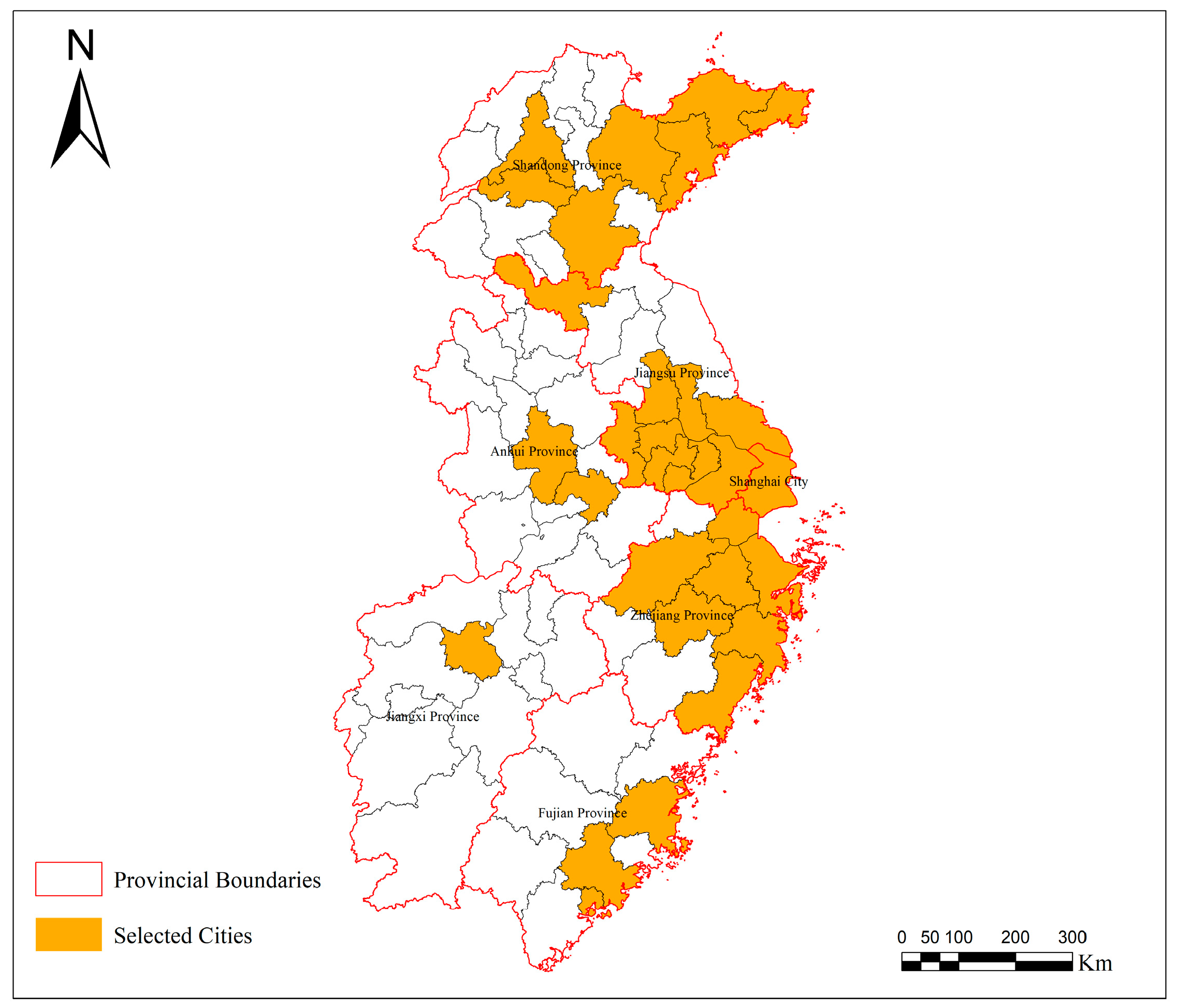
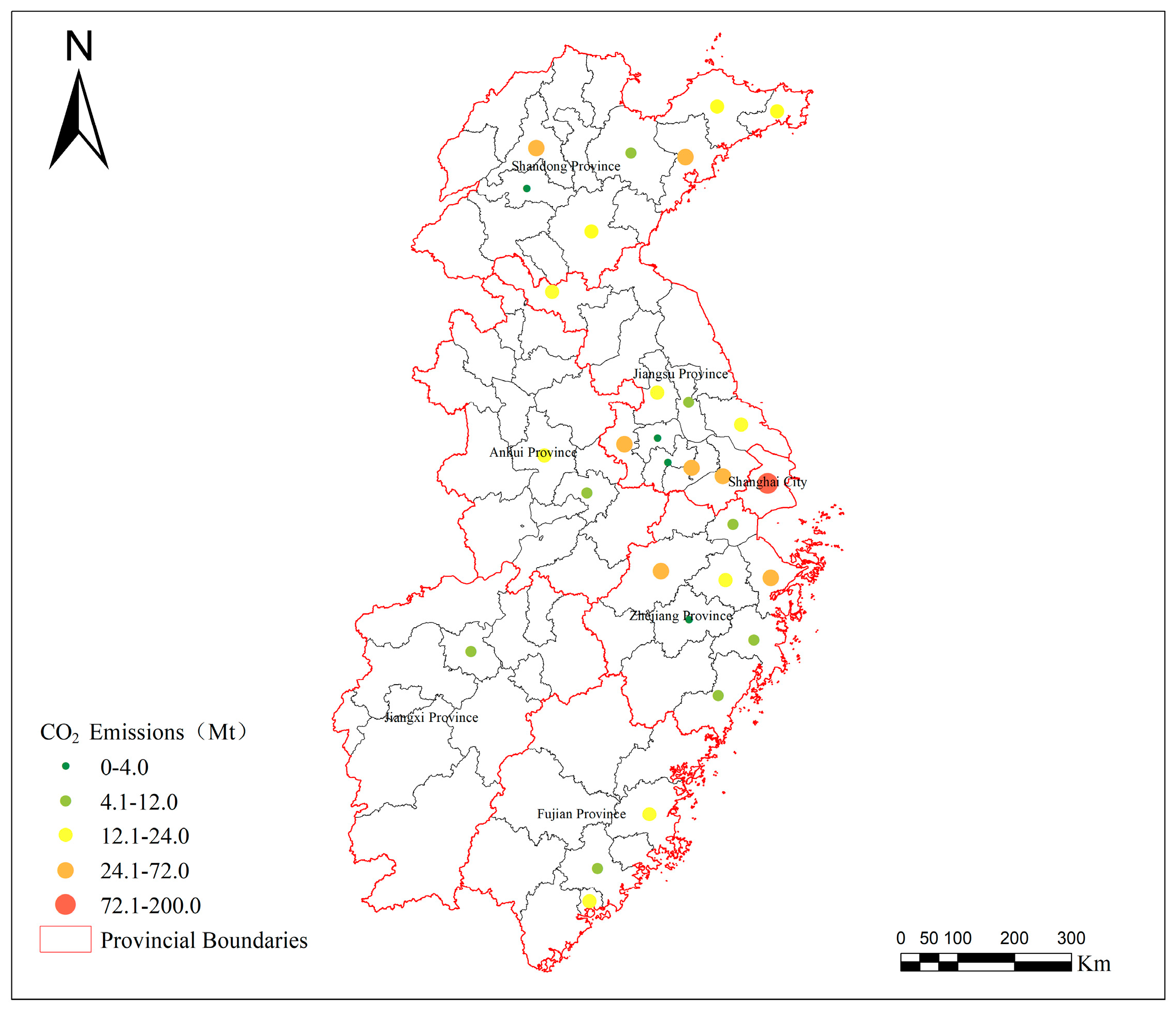
2.1. Study Area

East China stands as one of China’s foremost economically developed regions, including eight provinces and cities such as Shanghai, Jiangsu, Zhejiang, Anhui, Jiangxi, Fujian, Shandong, and Taiwan (data missing, not studied at the moment). In 2019, the region’s GDP accounted for 38.02% of China’s total and its population was 29.97%. However, rapid economic development has also brought about the problem of high energy consumption. In 2019, East China represented 29.69% of the total energy consumption of China, ranking it first among the seven major regions in China. High energy consumption means high CO₂ emissions. At the same time, with a plethora of urban agglomerations in the East China region, the rapid urban growth will undeniably result in significant environmental challenges associated with increased emissions. Therefore, 30 cities in East China were selected as the specific study area. The specific study area is shown in Figure 1.

2.2. Data

The data used in this study include CO₂ emission and spatial distribution data of buildings in East China in 2019 (Figure 2). The CO₂ emission data come from ODIAC (Open Source Data Inventory for Anthropogenic CO₂) [32,33], which is comprehensive, combined with multiple source remote sensing data, nonpoint source data, and fossil fuel consumption statistics for the estimation of CO₂ emission, and have been verified for accuracy.

The spatial distribution data of buildings come from the Gaode map, which includes information such as building location, building outline, and number of floors.

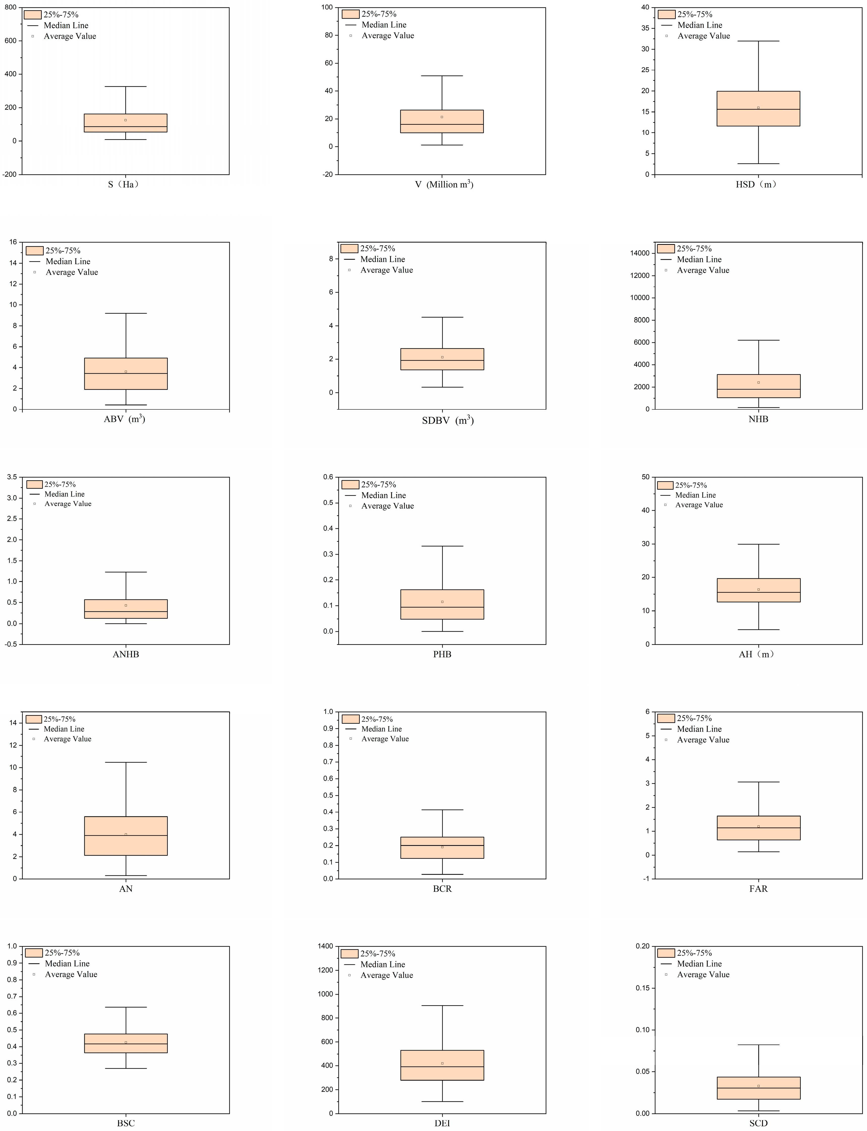
2.3. Quantification of Urban Three-Dimensional Spatial Structure

To illustrate the tridimensional spatial characteristics of cities, indicators such as building height, density, volume, coefficient of shape of the building, distribution uniformity index, spatial congestion, building area, building volume, average building volume, standard deviation of building volume, and the number and percentage of high-rise buildings are selected to quantify the three-dimensional spatial structure of the city [28,29,30]. According to China’s high-rise building design code, residential buildings with a house height of more than 28 m and other high-rise civil buildings with a building height of more than 24 m of concrete structure buildings are categorized as high-rise buildings. The building volume (V) is the sum of the volumes of all buildings within the unit boundaries and is used to quantify the degree of expansion of urban buildings in three-dimensional space. Employing the Building Space Coefficient (BSC), the measurable connection between building area and volume is articulated, which can reflect the thermal variability of the building. The distributional uniformity index (DEI) is used to show the distribution of buildings in a three-dimensional space to quantify the uniformity of buildings in a three-dimensional space, thus reflecting the irregularity of urban three-dimensional spatial structures. The Building Coverage Ratio (BCR) represents the building coverage within the scope of the research unit, and the FAR is the ratio of the total floor area to the unit area within the unit boundaries and is used to quantify the intensity of development within the unit. The spatial crowding degree (SCD) is used to represent the congestion of a building in a three-dimensional space. These indicators can be used to quantify the three-dimensional structural characteristics of cities. To provide a basis for further research on urban planning and development,

Table 1. Quantitative indicators of the three-dimensional architectural structure of the urban area.

Indicator	Abbreviation	Formula	Description
Building footprint	S	$S={\displaystyle \sum _{i=1}^n}{S}_i$	A = Area of the research unit N = Number of buildings S = building footprint H = building height F = Number of floors in the building Havg = Average building height Vavg = Average building volume P = building perimeter
Total building volume	V	$V={\displaystyle \sum _{i=1}^n}{S_{i}H}_i$
Average building volume	ABV	$ABV={\displaystyle \frac{\sum _{i=1}^n{S_{i}H}_i}{N}}$
Standard deviation of building volume	SDBV	$SDBV=\sqrt{{\displaystyle \frac{\sum _{i=1}^n{(V_i-V_{avg})}^2}{N}}}$
Number of high-rise buildings	NHB	— —
Average number of high-rise buildings	ANHB	$ANHB={\displaystyle \frac{NHB}{A}}$
Percentage of high-rise buildings	PHB	$PHB={\displaystyle \frac{NHB}{N}}$
Average building height	AH	$AH={\displaystyle \frac{\sum _{i=1}^n{H}_i}{N}}$
Standard deviation of building height	HSD	$HSD=\sqrt{{\displaystyle \frac{\sum _{i=1}^n{(H_i-H_{avg})}^2}{N}}}$
Average number of buildings	AN	$AN={\displaystyle \frac{N}{A}}$
Building coverage ratio	BCR	$BCR={\displaystyle \frac{\sum _{i=1}^n{S}_i}{A}}$
Floor area ratio	FAR	$FAR={\displaystyle \frac{\sum _{i=1}^n{S_{i}F}_i}{A}}$
Building shape coefficient	BSC	$BSC={\displaystyle \frac{\sum _{i=1}^n\frac{{P_{i}H}_i+S_i}{{S_{i}H}_i}}{N}}$
Distribution evenness index	DEI	$DEI=\sqrt{{\displaystyle \frac{\sum _{i=1}^n{(V_i-V_{avg})}^2}{A}}}$
Spatial congestion degree	SCD	$SCD={\displaystyle \frac{\sum _{i=1}^n{S_{i}H}_i}{max\left(H_i\right)\ast A}}$

describes the quantitative spatial indicators of three-dimensional building structures.

2.4. Data Preprocessing

By normalizing spatial indicator data, it is possible to eliminate discrepancies, improve comparability, and reduce the impact of outliers. It also improves the performance of machine learning models for better use in analysis, evaluation, and decision-making processes. The approach for normalized calculation is provided below:

$$Y={\displaystyle \frac{\mathrm{X}-X_{min}}{X_{max}-X_{min}}}$$

(1)

where X is the spatial indicator data, X_min is the minimum spatial indicator data, X_max is the maximum spatial indicator data, and Y is the normalized spatial indicator data.

To detect the correlation between spatial indicators and CO₂, we performed a Pearson test using SPSS software to determine which spatial indicator correlates most strongly with CO₂ emissions based on the correlation coefficient. The correlation coefficient is expressed as follows:

$$R={\displaystyle \frac{\sum \left(x-\overline{x}\right)\left(y-\overline{y}\right)}{\sqrt{\sum {(x-\overline{x})}^2}\sqrt{\sum {(y-\overline{y})}^2}}}$$

(2)

where X is the spatial indicator data; X_min is the minimum spatial indicator data; X_max is the maximum spatial indicator data; and Y is the normalized spatial indicator data. R stands for the correlation coefficient, with $\overline{x}$ and $\overline{y}$ being the arithmetic means of the variables x and y, correspondingly.

2.5. Methodologies

2.5.1. Backpropagation Neural Network (BP)

BP is one of the most widely used artificial neural networks that mainly deals with classification and regression problems in different fields. The structural design of BP is manifested as a multilayer network topology, including input, hidden, and output layers [34].

In this study, the BP training process is mainly based on the error-based backpropagation mechanism, and 478 sets of data containing 15 three-dimensional spatial indicators and carbon emissions are fed through the input layer, dividing the training set and the test set according to the ratio 7:2. The data are calculated by the hidden layer network to output the predicted value and compare it with the real value, the error is calculated and then back-propagated to the input layer, the weights and bias terms in the network are updated by using the gradient descent method to reduce the error, and the final output is the predicted value of carbon emissions. The model is set up with a six-layer network architecture, in which the hidden layer contains 10 neurones; the number of iterations is 300, and the training error threshold and learning rate are set to 0.01.

2.5.2. Random Forest (RF)

RF is a Bagging ensemble theory based on CART (Classification and Regression Tree) decision trees proposed by Breimanl in 2001. It combines an improved ensemble learning method based on the theory of stochastic subspace theoretical models, mainly used for classification and regression problems [35].

In this study, the dataset is input by the input layer, divided into a test set and training set according to a 7:2 ratio, and multiple samples are drawn from the training set using the Bootstrap resampling method. Decision tree modeling is performed for each sample taken, multiple decision trees are formed for prediction, and after testing the prediction results using the test set, the regression results of the multiple internal decision trees are averaged to output the predicted value of carbon emissions. Iterative optimization determines the number of decision trees to be 200 and the number of leaves in each tree to be 40.

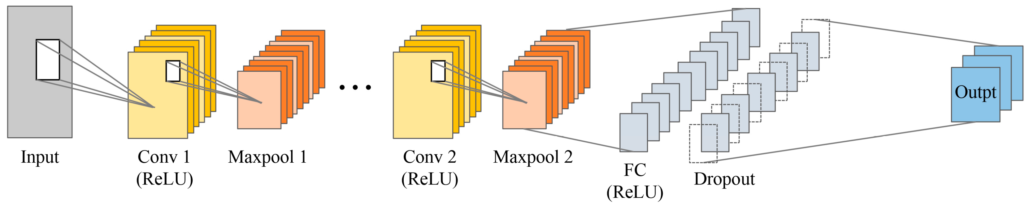
2.5.3. Convolutional Neural Network (CNN)

CNNs can efficiently extract features from the input data by performing convolutional operations and can reduce the number of parameters in this way, a feature that helps to enhance the generalization ability of the network and reduce the risk of overfitting. The main structure of a CNN includes an input layer, a convolutional layer, a pooling layer, a fully connected layer, and an output layer [36].

In this paper, the sample data are input through the input layer, the convolution layer is mainly used to extract the features of the input data, the pooling layer compresses the features of the output of the convolution operation to achieve the effect of reducing the dimensionality, which is used to solve the overfitting problem, and the activation layer performs a nonlinear transformation on the output of the convolution layer and adjusts the weights moderately. The fully connected layer integrates all the features used in the output layer to output the predicted value of carbon emissions. Due to the possible overfitting of the neural network, we introduced the dropout and early stop strategies and chose Adam’s algorithm to optimize the learning rate, using the ReLU function as the activation function. Through iterative optimization, it was determined that the dropout rate was set to 0.2, the initial learning rate was 0.01, the maximum number of iterations was 800, the minimum training batch was 30, the learning rate dropout period was set to 400, and the dropout factor was 0.2. The structure is shown in Figure 3.

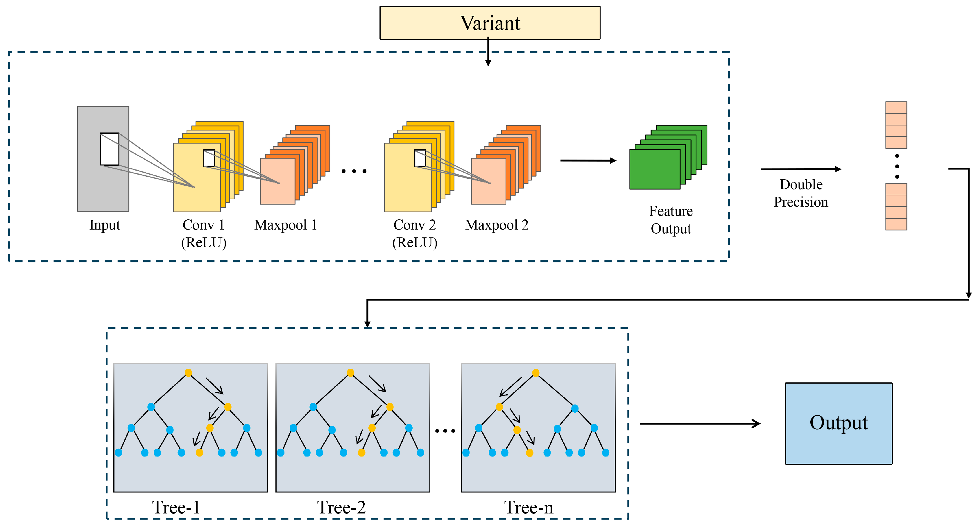
2.5.4. Convolutional Neural Network–Random Forest (CNN-RF)

The main advantage of CNN is that it extracts important data features and reduces noise, but it requires a large amount of data to achieve good model performance [37], and cannot avoid the effect of autocorrelation of the input data on the output results. In contrast, RF does not require a high number of samples, still achieves good regression results with a small amount of data [38], and is not affected by multicollinearity between the data [39]. Due to the small dataset in this paper, this study chooses to use CNN for feature extraction and RF for regression prediction, combining the CNN-RF hybrid model to build a carbon emission prediction model by inputting datasets containing spatial indicators and carbon emissions.

In this study, CNN-RF is based on the CNN model, the data features are extracted by the CNN, the output of the CNN in the “pool-2” is taken as the new features, the data type is converted and input into the RF, and the predicted value of the carbon emission is output by the regression of the RF decision tree. Compared with the CNN and RF models, this model modifies some parameters in the CNN, in which the initial learning rate is changed to 0.01, the maximum number of iterations is 400, the minimum training batch is 80, the learning rate descent period is set to 200, and the descent factor is 0.1, and there is no change in the RF parameters. The CNN-RF structure is shown in Figure 4.

2.6. Model Evaluation

The coefficient of determination (R²), root mean square error (RMSE), and residual prediction deviation (RPD) are used for the validation of model accuracy. R² represents the degree of correlation between the predicted values and the true values, and the larger R² is, the higher the correlation is. RMSE represents the error between the predicted values and the true values, and a smaller RMSE indicates that the model predicts the results more accurately. RPD is the ratio of the standard deviation of the true value to the standard error of the predicted value, which can be used as a comprehensive measure of the model’s predictive ability. When RPD < 1.4, 1.4 < RPD < 2, or RPD > 2, it indicates that the predictive ability of the model is poor, average, or good, respectively. The formulae are as follows:

$$R^2={\displaystyle \frac{\sum _{n=i}^n{\left({\widehat{y}}_i-{\overline{y}}_i\right)}^2}{\sum _{n=i}^n{\left(y_i-{\overline{y}}_i\right)}^2}}$$

(3)

$$RMSE=\sqrt{{\displaystyle \frac{\sum _{n=i}^n{\left(y_i-{\widehat{y}}_i\right)}^2}{n}}}$$

(4)

$$RPD={\displaystyle \frac{SD}{RMSE}}$$

(5)

where ${\widehat{y}}_i$ is the projected CO₂ emissions, $y_i$ is the measured CO₂ emissions, $\overline{y}$ is the average CO₂ emissions, n denotes the sample size, and SD is the standard deviation.

2.7. Model Building

To calculate the three-dimensional spatial structure of cities and distinguish its characteristics, we used the administrative boundaries of townships and streets as the criteria for the division of the study unit. A total of 531 datasets were used in this study. The 15 three-dimensional spatial indicators were selected as the independent variables for quantification, and the total annual CO₂ emissions were considered the dependent variable. During sample data processing, the data were randomly selected in a ratio of 7:2:1 and divided into training sets, testing sets, and validation sets for model training. The evaluation of the model employs three key performance indicators: R², RMSE, and RPD. The specific datasets and processes are shown in

Table 2. Model data partition.

Sample Set	Number	Min	Max	Standard Deviation
Training Set	372	1.64	179.95	28.37
Test Set	106	3.52	132.91	26.80
Validation Set	53	1.82	147.22	43.97

and Figure 5.

3. Results

3.1. Relevant Analysis

Using the Pearson correlation coefficient technique, this research performs an analysis to determine the correlation between CO₂ emissions and 15 three-dimensional spatial indicators. Based on the calculations, it was found that CO₂ emissions in the region were significantly negatively correlated with the parameters ANHB, ABV, AH, AN, BCR, FAR, DEI, and SCD, and showed a positive correlation with the indicators S, V, HSD, ABV, SDBV, NHB, PHB, and BSC. These are shown in

Table 3. Correlation coefficient between CO₂ and spatial indicators.

S	V	HSD	ABV	SDBV
0.720	0.709	0.078	−0.120	0.169
NHB	ANHB	PHB	AH	AN
0.584	−0.219	0.009	−0.065	−0.303
BCR	FAR	BSC	DEI	SCD
−0.389	−0.375	0.117	−0.169	−0.421

.

In urban areas, when the average number of buildings, building height, building coverage, and floor area ratio increases in an urban area, CO₂ emissions decrease accordingly. As the values of S, V, HSD, ABV, SDBV, NHB, and PHB increase, CO₂ emission rises. Among them, S has the most evident impact on CO₂ emissions, with an absolute correlation coefficient of 0.720, higher than all other indicators. The correlation coefficients of V, NHB, SCD, BCR, FAR, and AN with CO₂ emissions are 0.709, 0.584, 0.421, 0.389, 0.375, and 0.303. This demonstrates the significant link between the three-dimensional spatial structure of cities and their corresponding CO₂ emission levels.

3.2. Variable Analysis

According to the CO₂ emissions datasets and Figure 2 for the study area, CO₂ emissions are generally higher in the areas of the city centre and gradually decrease as they extend to the fringes and suburbs of the city. Dense built-up areas are the highest emitters of CO₂ within cities, while sparse fringe and suburban areas emit less.

In this study, we computed a series of spatial indicators using specific building data for each city. The distribution of these indicators across cities is visualized in the form of a box plot, as depicted in Figure 6. Owing to disparities in economic activity and geographic contexts between cities, the figures for diverse indicators show considerable variance among urban centers. For example, in BCR, the box plot shows a centralized distribution around 0.19, with an overall range mainly between 0.10 and 0.25. The centralized value of the number of buildings for indicator N is 2419. The minimum number of buildings is 178, and the maximum is 17,281. In the BSC, the concentration value is 0.43, with an upper limit of 0.27 and a lower limit of 0.70. Other spatial indicators, such as N, S, V, AH, and AVB, also exhibit their distributional characteristics across cities. The distribution ranges of the three-dimensional spatial indicators quantified in this study are generally consistent with the findings of Xu and Dong et al. [29,31].

3.3. Model Analysis

Through a comparative examination of

Table 4. Accuracy evaluation of four models.

Model Type	R2	RMSE	RPD
BP	0.68	18.00	1.49
RF	0.77	13.44	1.99
CNN	0.81	12.25	2.19
CNN-RF	0.85	10.60	2.53

and Figure 7, insights can be gained into the predictive performance of the BP, RF, CNN, and CNN-RF models in estimating CO₂ emissions. With an RPD value over 1.4 for each of the four models, it is evident that they all hold estimation capabilities, and the BP model shows relatively average predictive performance. According to the data presented in Table 3 and Figure 6, the R² is recorded at 0.68, the RMSE stands at 18.00, and the RPD is calculated as 1.49. These results indicate that the BP model has relatively low precision in fitting and predicting CO₂ emissions. Compared with it, the RF and CNN models exhibit superior performance. This is evidenced by their R² values rising to 0.77 and 0.81, RMSE decreasing to 13.44 and 12.25, and RPD increasing to 1.99 and 2.19, respectively. These findings suggest that the RF and CNN models demonstrate robustness and enhanced predictive precision. The CNN-RF model performed best in predicting CO₂ emissions. Significant improvements were observed in all assessment indicators. R² reached 0.85, marking an increase of approximately 4.94% over CNN; RMSE decreased to 10.60, reflecting a decrease of about 13.47%; and RPD increased to 2.53, showing a rise of 15.53%. These results demonstrate the superior predictive power of the CNN and CNN-RF models in forecasting CO₂ emissions.

In the testing phase, the R² values of both the CNN and CNN-RF models exceeded 0.80, and both models were validated. According to

Table 5. Accuracy evaluation of model verification.

Model Type	R2	RMSE	RPD
CNN	0.73	25.54	1.72
CNN-RF	0.82	22.32	1.97

and Figure 8, it is evident that the R², RMSE, and RPD of both models decreased during the validation process compared to the testing phase, with a smaller decrease for the CNN-RF model. Compared with CNN, the CNN-RF model has a 12.33% higher metric R², 12.61% lower RMSE, and 11.63% higher RPD in the validation model of CO₂ emissions. It indicates that CNN-RF demonstrates superior predictive capabilities.

4. Discussion

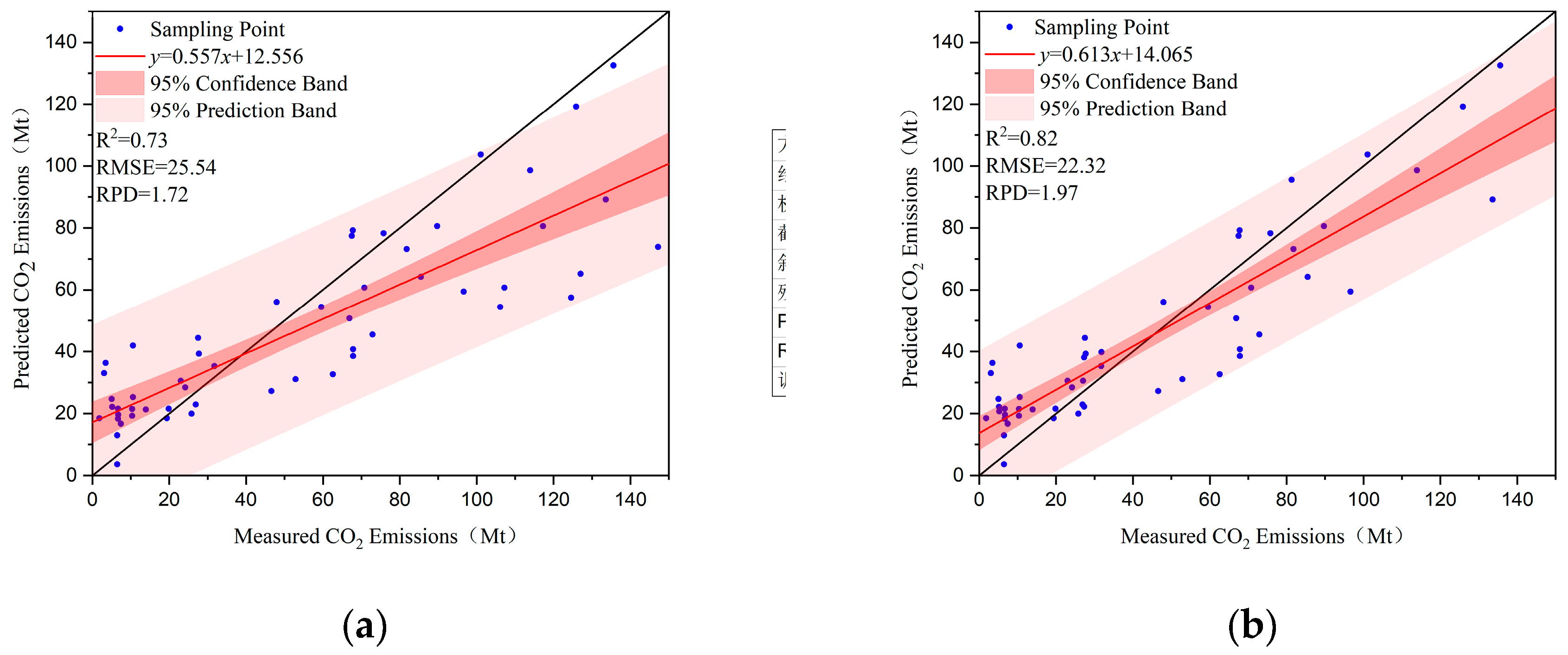
4.1. Comparative Analysis of Models

Among the four machine learning models, the CNN-RF model achieves the highest performance. Its R², RMSE, and RPD values were optimal during testing and validation. During the execution of model predictions, compared to using spatial data directly, the prediction accuracy is significantly improved when leveraging spatial data with high feature extraction obtained from the CNN.

While the BP model is capable of addressing nonlinear issues, it is limited by its structure and training methods. It may not effectively capture deep and complex features when modeling the relationship between complex spatial indicators and CO₂ emissions.

RF uses more sophisticated classification methods to avoid over-matching. However, spatial data prediction requires extensive preprocessing of input features, which often results in inaccurate model predictions.

CNNs can automatically extract the spatial features of the input data, which reduces the number of parameters of the model and enhances the computing power of the model. However, in CNN-based prediction, a large amount of training data is usually required to extract informative high-level spatial features, and the lack of sufficient training data can cause the model to produce poor prediction accuracy. In addition, the convolutional layer’s focus on localized features and the difficulty in capturing all the information in the input data may also contribute to the reduced accuracy of predictive forecasting.

The advantage of CNN-RF lies in its ability to combine CNN models with RF models. This approach allows combining simple classifiers with feature extraction capabilities with complex classifiers that lack feature extractors to fully utilize the strengths of the model. Although RF is not as good as some deep learning models when dealing with large-scale datasets, with the high-featured data input after CNN extraction, RF can take full advantage of a large number of decision trees while using unselected samples to estimate the effect of missing values and avoid being affected by local features.

4.2. Impact of Three-Dimensional Spatial Structure on CO₂ Emissions

After comparing the optimal prediction model CNN-RF, the importance of each independent variable in CNN-RF is evaluated, and the score results are shown in Figure 9. The results are similar to those obtained by Pearson’s correlation coefficient method. Combining the scores and coefficient results, S, V, and NHB are the most important factors affecting CO₂ emissions in the study area on the township scale (street). The continuous outward expansion of cities during the urbanization process is primarily responsible for this phenomenon. The significant increase in construction land has diminished non-construction land, including farmland, forest land, and grassland. This shift has resulted in elevated CO₂ emissions and reduced carbon storage in vegetation. With the increase in urban population, buildings are expanding. Major cities are increasingly inclined to construct taller and larger buildings to accommodate the growing demand. This also leads to the concentration of large numbers of people whose daily activities in buildings generate significant energy consumption. For instance, high-rise buildings affect the lighting of the ground floor, increasing the demand for lighting. The concentration of the population leads to traffic congestion, which slows vehicle movement and increases CO₂ emissions. The height of the building has a smaller but contributing effect on CO₂ emissions compared to the total volume of the building, a result that validates previous findings [27]. Tall buildings are more likely to receive sunlight and heat, leading to an increase in building temperature. Consequently, residents will consume more energy to maintain a comfortable living environment. Additionally, buildings that are too tall require elevators to ensure access, which inevitably leads to more CO₂ emissions. Therefore, the heights of the buildings should be reasonably controlled in the urban planning stage.

In contrast, AN and BCR, which represent the density of buildings in a given area, are negatively correlated with CO₂ emissions. This correlation suggests that the urban fabric is becoming more spatially compact as building coverage and the number of buildings within the study unit increase, which will favor the reduction of CO₂ emissions. This is consistent with the compact development perspective [40,41]. The concept posits that the urban layout should be concentrated and centralized, rather than excessively scattered. Compact urban structures contribute to sustainable development. Centralized services reduce energy consumption and waste, shorten commute distances, reduce reliance on automobile transport, and preserve non-construction land outside of the city. These factors collectively reduce CO₂ emissions.

SCD and FAR represent the compactness of buildings in the third dimension, although high-density urban configurations obstruct airflow, reduce sunlight penetration, and hinder urban ventilation. However, in the context of townships and neighborhoods, high SCD and FAR are beneficial in reducing CO₂ emissions in urban areas. This discovery aligns with the concept of compact development mentioned earlier. On larger scales, concentrating on three dimensions also helps reduce CO₂ emissions.

In addition, the DEI hurts CO₂ emissions, but its impact is relatively minor compared to other factors. The DEI serves as a spatial indicator that illustrates the evenness of the distribution of urban buildings in a three-dimensional space. A higher DEI value indicates a more irregular urban structure. The negative correlation between the DEI and CO₂ emissions suggests that an irregular three-dimensional urban spatial layout can help reduce CO₂ emissions. Irregular urban structures allow for greater spacing, better ventilation, and more daylight than uniform urban structures, which helps to reduce energy requirements for cooling and lighting. Therefore, at the township (street) scale, the irregular three-dimensional urban structure helps to reduce CO₂ emissions.

Finally, SDBV, BSC, and HSD contribute to urban CO₂ emissions, while AH, ABV, and ANHB help reduce CO₂ emissions in cities. However, these factors have minimal impact on CO₂ emissions on the township scale (street).

5. Conclusions

This study examines urban agglomeration in East China and integrates urban building data and anthropogenic CO₂ emissions data using a machine learning model to explore the relationship between the three-dimensional spatial structure of the city and CO₂ emissions. By comparing and analyzing the BP, RF, CNN, and CNN-RF models, we assess the predictive capabilities of these models for CO₂ emissions. Furthermore, we explore the primary three-dimensional spatial factors that influence CO₂ emissions. The main conclusions are as follows.

Compared to the BP, RF, and CNN models, the CNN-RF model in the CO₂ emissions training model shows R² indicators that are 20.00%, 9.41%, and 4.71% higher, respectively. The RMSE decreases by 69.81%, 26.79%, and 15.57%. In the model validation phase, the CNN-RF model exhibited a 12.33% higher R² metric and a 12.61% lower RMSE in the CO₂ emissions validation model compared to CNN. The predictive capacity of CNN-RF exceeds that of other models.

Combining the results of the Pearson’s correlation coefficient method and the CNN-RF model, it is evident that CO₂ emissions are closely related to the three-dimensional spatial structure. CO₂ emissions exhibit a negative correlation with ABV, ANHB, AH, AN, BCR, FAR, DEI, and SCD. Conversely, they show a positive correlation with S, V, HSD, SDBV, NHB, PHB, and BSC. Among these indicators, V, S, and NHB have the most significant influence on CO₂ emissions, surpassing the impact of other factors. It can be observed that strategically planning the three-dimensional spatial structure of a city can help to develop low-carbon cities.

Despite its contributions, this study is not devoid of restrictions. Firstly, the identification of pertinent variables was influenced by the bounds of data obtainability, and building data acquisition was not comprehensive enough. Additionally, this study primarily investigated the relationship between the three-dimensional spatial structure of the city and CO₂ emissions, ignoring variables such as building type, urban traffic flow, and population density that can affect urban CO₂ emissions. Finally, more studies are needed to explore the potential impact of choosing different research units on prediction results. Therefore, future studies will be more focused on individual cities, considering the use of web crawlers to obtain more accurate and comprehensive data, and verifying the accuracy of the data based on satellite images.

References

1. Silva, M.; Oliveira, V.; Leal, V. Urban Form and Energy Demand. J. Plan. Lit. 2017, 32, 346–365. [Google Scholar] [CrossRef]
2. Cai, B.; Liang, S.; Zhou, J.; Wang, J.; Cao, L.; Qu, S.; Xu, M.; Yang, Z. China high resolution emission database (CHRED) with point emission sources, gridded emission data, and supplementary socioeconomic data. Resour. Conserv. Recycl. 2018, 129, 232–239. [Google Scholar] [CrossRef]
3. Wang, S.; Liu, X. China’s city-level energy-related CO2 emissions: Spatiotemporal patterns and driving forces. Appl. Energy 2017, 200, 204–214. [Google Scholar] [CrossRef]
4. Wang, S.; Liu, X.; Zhou, C.; Hu, J.; Ou, J. Examining the impacts of socioeconomic factors, urban form, and transportation networks on CO2 emissions in China’s megacities. Appl. Energy 2017, 185, 189–200. [Google Scholar] [CrossRef]
5. Wakiyama, T.; Zusman, E. The impact of electricity market reform and subnational climate policy on carbon dioxide emissions across the United States: A path analysis. Renew. Sustain. Energy Rev. 2021, 149, 111337. [Google Scholar] [CrossRef]
6. Fan, T.; Chapman, A. Policy Driven Compact Cities: Toward Clarifying the Effect of Compact Cities on Carbon Emissions. Sustainability 2022, 14, 12634. [Google Scholar] [CrossRef]
7. Ribeiro, H.V.; Rybski, D.; Kropp, J.P. Effects of changing population or density on urban carbon dioxide emissions. Nat. Commun. 2019, 10, 3204. [Google Scholar] [CrossRef] [PubMed]
8. Domon, S.; Hirota, M.; Kono, T.; Managi, S.; Matsuki, Y. The long-run effects of congestion tolls, carbon tax, and land use regulations on urban CO2 emissions. Reg. Sci. Urban Econ. 2022, 92, 103750. [Google Scholar] [CrossRef]
9. Tang, J.; Gong, R.; Wang, H.; Liu, Y. Scenario analysis of transportation carbon emissions in China based on machine learning and deep neural network models. Environ. Res. Lett. 2023, 18, 064018. [Google Scholar] [CrossRef]
10. Luna, T.F.; Uriona-Maldonado, M.; Silva, M.E.; Vaz, C.R. The influence of e-carsharing schemes on electric vehicle adoption and carbon emissions: An emerging economy study. Transp. Res. Part D Transp. Environ. 2020, 79, 102226. [Google Scholar] [CrossRef]
11. Li, Z.; Wang, F.; Kang, T.; Wang, C.; Chen, X.; Miao, Z.; Zhang, L.; Ye, Y.; Zhang, H. Exploring differentiated impacts of socioeconomic factors and urban forms on city-level CO2 emissions in China: Spatial heterogeneity and varying importance levels. Sustain. Cities Soc. 2022, 84, 104028. [Google Scholar] [CrossRef]
12. Shahbaz, M.; Nasir, M.A.; Hille, E.; Mahalik, M.K. UK’s net-zero carbon emissions target: Investigating the potential role of economic growth, financial development, and R&D expenditures based on historical data (1870–2017). Technol. Forecast. Soc. Chang. 2020, 161, 120255. [Google Scholar] [CrossRef]
13. Hailemariam, A.; Dzhumashev, R.; Shahbaz, M. Carbon emissions, income inequality and economic development. Empir. Econ. 2019, 59, 1139–1159. [Google Scholar] [CrossRef]
14. Hong, S.; Hui, E.C.-M.; Lin, Y. Relationship between urban spatial structure and carbon emissions: A literature review. Ecol. Indic. 2022, 144, 109456. [Google Scholar] [CrossRef]
15. Lu, X.; Zhang, Y.; Li, J.; Duan, K. Measuring the urban land use efficiency of three urban agglomerations in China under carbon emissions. Environ. Sci. Pollut. Res. 2022, 29, 36443–36474. [Google Scholar] [CrossRef]
16. Sarkodie, S.A.; Owusu, P.A.; Leirvik, T. Global effect of urban sprawl, industrialization, trade and economic development on carbon dioxide emissions. Environ. Res. Lett. 2020, 15, 034049. [Google Scholar] [CrossRef]
17. Wu, Y.; Li, C.; Shi, K.; Liu, S.; Chang, Z. Exploring the effect of urban sprawl on carbon dioxide emissions: An urban sprawl model analysis from remotely sensed nighttime light data. Environ. Impact Assess. Rev. 2022, 93, 106731. [Google Scholar] [CrossRef]
18. Sufyanullah, K.; Ahmad, K.A.; Sufyan Ali, M.A. Does emission of carbon dioxide is impacted by urbanization? An empirical study of urbanization, energy consumption, economic growth and carbon emissions—Using ARDL bound testing approach. Energy Policy 2022, 164, 112908. [Google Scholar] [CrossRef]
19. Hanif, I. Impact of fossil fuels energy consumption, energy policies, and urban sprawl on carbon emissions in East Asia and the Pacific: A panel investigation. Energy Strategy Rev. 2018, 21, 16–24. [Google Scholar] [CrossRef]
20. Ding, S.; Liu, S.; Chang, M.; Lin, H.; Lv, T.; Zhang, Y.; Zeng, C. Spatial Optimization of Land Use Pattern toward Carbon Mitigation Targets—A Study in Guangzhou. Land 2023, 12, 1903. [Google Scholar] [CrossRef]
21. Xia, C.; Zhang, J.; Zhao, J.; Xue, F.; Li, Q.; Fang, K.; Shao, Z.; Zhang, J.; Li, S.; Zhou, J. Exploring potential of urban land-use management on carbon emissions—A case of Hangzhou, China. Ecol. Indic. 2023, 146, 109902. [Google Scholar] [CrossRef]
22. Wang, G.; Han, Q.; de Vries, B. The multi-objective spatial optimization of urban land use based on low-carbon city planning. Ecol. Indic. 2021, 125, 107540. [Google Scholar] [CrossRef]
23. Wang, X.; Cai, Y.; Liu, G.; Zhang, M.; Bai, Y.; Zhang, F. Carbon emission accounting and spatial distribution of industrial entities in Beijing—Combining nighttime light data and urban functional areas. Ecol. Inform. 2022, 70, 101759. [Google Scholar] [CrossRef]
24. Zheng, Y.; Du, S.; Zhang, X.; Bai, L.; Wang, H. Estimating carbon emissions in urban functional zones using multi-source data: A case study in Beijing. Build. Environ. 2022, 212, 108804. [Google Scholar] [CrossRef]
25. Falahatkar, S.; Rezaei, F. Towards low carbon cities: Spatio-temporal dynamics of urban form and carbon dioxide emissions. Remote Sens. Appl. Soc. Environ. 2020, 18, 100317. [Google Scholar] [CrossRef]
26. Cucchiella, F.; Rotilio, M. Planning and prioritizing of energy retrofits for the cities of the future. Cities 2021, 116, 103272. [Google Scholar] [CrossRef]
27. Mostafavi, F.; Tahsildoost, M.; Zomorodian, Z. Energy efficiency and carbon emission in high-rise buildings: A review (2005–2020). Build. Environ. 2021, 206, 108329. [Google Scholar] [CrossRef]
28. Resch, E.; Bohne, R.A.; Kvamsdal, T.; Lohne, J. Impact of Urban Density and Building Height on Energy Use in Cities. Energy Procedia 2016, 96, 800–814. [Google Scholar] [CrossRef]
29. Xu, X.; Ou, J.; Liu, P.; Liu, X.; Zhang, H. Investigating the impacts of three-dimensional spatial structures on CO2 emissions at the urban scale. Sci. Total Environ. 2021, 762, 143096. [Google Scholar] [CrossRef]
30. Lin, J.; Lu, S.; He, X.; Wang, F. Analyzing the impact of three-dimensional building structure on CO2 emissions based on random forest regression. Energy 2021, 236, 121502. [Google Scholar] [CrossRef]
31. Dong, Q.; Huang, Z.; Zhou, X.; Guo, Y.; Scheuer, B.; Liu, Y. How building and street morphology affect CO2 emissions: Evidence from a spatially varying relationship analysis in Beijing. Build. Environ. 2023, 236, 110258. [Google Scholar] [CrossRef]
32. Oda, T.; Maksyutov, S. A very high-resolution (1 km × 1 km) global fossil fuel CO2; emission inventory derived using a point source database and satellite observations of nighttime lights. Atmos. Chem. Phys. 2011, 11, 543–556. [Google Scholar] [CrossRef]
33. Oda, T.; Maksyutov, S.; Andres, R.J. The Open-source Data Inventory for Anthropogenic CO2, version 2016 (ODIAC2016): A global monthly fossil fuel CO2 gridded emissions data product for tracer transport simulations and surface flux inversions. Earth Syst. Sci. Data 2018, 10, 87–107. [Google Scholar] [CrossRef] [PubMed]
34. Buscema, M. Back Propagation Neural Networks. Subst. Use Misuse 1998, 33, 233–270. [Google Scholar] [CrossRef]
35. Breiman, L. Random forests. Mach. Learn. 2001, 45, 5–32. [Google Scholar] [CrossRef]
36. Fang, D.; Zhang, X.; Yu, Q.; Jin, T.C.; Tian, L. A novel method for carbon dioxide emission forecasting based on improved Gaussian processes regression. J. Clean. Prod. 2018, 173, 143–150. [Google Scholar] [CrossRef]
37. Alzubaidi, L.; Zhang, J.; Humaidi, A.J.; Al-Dujaili, A.; Duan, Y.; Al-Shamma, O.; Santamaría, J.; Fadhel, M.A.; Al-Amidie, M.; Farhan, L. Review of deep learning: Concepts, CNN architectures, challenges, applications, future directions. J. Big Data 2021, 8, 53. [Google Scholar] [CrossRef] [PubMed]
38. Yang, S.; Gu, L.; Li, X.; Jiang, T.; Ren, R. Crop Classification Method Based on Optimal Feature Selection and Hybrid CNN-RF Networks for Multi-Temporal Remote Sensing Imagery. Remote Sens. 2020, 12, 3119. [Google Scholar] [CrossRef]
39. Li, T.; Leng, J.; Kong, L.; Guo, S.; Bai, G.; Wang, K. DCNR: Deep cube CNN with random forest for hyperspectral image classification. Multimed. Tools Appl. 2018, 78, 3411–3433. [Google Scholar] [CrossRef]
40. Makido, Y.; Dhakal, S.; Yamagata, Y. Relationship between urban form and CO2 emissions: Evidence from fifty Japanese cities. Urban Clim. 2012, 2, 55–67. [Google Scholar] [CrossRef]
41. Sha, W.; Chen, Y.; Wu, J.; Wang, Z. Will polycentric cities cause more CO2 emissions? A case study of 232 Chinese cities. J. Environ. Sci. 2020, 96, 33–43. [Google Scholar] [CrossRef] [PubMed]
Figure 1. Distribution of study areas.
Sustainability 16 07623 g001
Figure 2. Total annual CO2 emissions in selected cities.
Sustainability 16 07623 g002
Figure 3. Schematic diagram of CNN network structure.
Sustainability 16 07623 g003
Figure 4. Schematic diagram of the CNN-RF network structure.
Sustainability 16 07623 g004
Figure 5. Flowchart of CO2 emission prediction.
Sustainability 16 07623 g005
Figure 6. Distribution map of the 15 spatial indicators.
Sustainability 16 07623 g006
Figure 7. Scatter diagrams depicting the results of estimations made by four distinct models: (a) BP, (b) RF, (c) CNN, and (d) CNN-RF. The obtained CO2 emissions represent the actual values, and the CO2 emissions computed by the model signify the predict values.
Sustainability 16 07623 g007
Figure 8. Verification scatter plots of the two models: (a) CNN and (b) CNN-RF. The obtained CO2 emissions represent the actual values, and the CO2 emissions computed by the model signify the predict values.
Sustainability 16 07623 g008
Figure 9. Scores of each spatial factor in the CNN-RF model.
Sustainability 16 07623 g009