Feasibility Study and Results from a Baseline Multi-Tool Active Seismic Acquisition for CO₂ Monitoring at the Hellisheiði Geothermal Field

Abstract

CO₂ capture and underground storage, combined with geothermal resource exploitation, are vital for future sustainable and renewable energy. The SUCCEED project explores the feasibility of re-injecting CO₂ into geothermal fields to enhance production and store CO₂ for climate change mitigation. This integration requires novel time-lapse monitoring approaches. At the Hellisheiði geothermal power plant in Iceland, seismic surveys utilizing conventional geophones and a permanent fiber-optic helically wound cable (HWC) for Distributed Acoustic Sensing (DAS) were designed to provide subsurface information and CO₂ monitoring. This work details the feasibility study and active seismic acquisition of the baseline survey, focusing on optical fiber sensitivity, seismic modeling, acquisition parameters, source configurations, and quality control. Post-acquisition signal analysis using a novel electromagnetic vibrating source is discussed. The integrated analysis of datasets from co-located sensors improved quality-control performance and geophysical interpretation. The study demonstrates the advantages of using densely sampled DAS data in space by multichannel processing. This experimental work highlights the feasibility of using HWC DAS cables in active surface seismic surveys with an environmentally friendly electromagnetic source, providing also a unique case of joint signal analysis from different types of sensors in high-temperature geothermal areas for energy and CO₂ storage monitoring in a time-lapse perspective.

1. Introduction

Carbon capture and storage (CCS) is crucial to enable reducing greenhouse gases as well as the utilization of renewable energy like geothermal power, which allows the reduction of CO₂ emissions; in the context of the European Green Deal, CCS plays a key role to deal with climate change and clean energy topics [1]. In fact, the adoption of the European Green Deal, the European Climate Law, and the subsequent proposals to increase energy and climate targets for 2030 have made carbon management technologies an important part of the EU decarbonization effort. Distributed Acoustic Sensing (DAS) is becoming increasingly popular in industry and academia for a variety of studies. There are many successful applications of DAS using existing telecommunication fibers, both on land and at sea. DAS has been used to record earthquakes [2,3,4,5], to reconstruct subsurface structures [6,7], to identify fault zones [8], to analyze oceanic microseismicity and tides [9], and to record thunderstorms [10], among others. High spatial and temporal resolution is helpful, but one of the main advantages of DAS is the ability to install fibers in boreholes and record seismic signals at depth. Continuous sampling along the trajectory of the borehole is possible with minimal disruption to operations; such resolution is difficult to achieve with conventional borehole tools [11]. DAS is used also for passive and active seismic monitoring applications. The directional sensitivity of standard fiber (acting as a single-component measurement) for DAS measurements is a critical issue when the cable is used for surface seismic surveys. The innovative helically wound cable (HWC) optimizes the measurement response in this situation, due to its broadside sensitivity.

Seismic monitoring has been used both in geothermal areas [12,13,14,15] and for CO₂ storage purposes [16,17]. Recently, Tsuji et al. [18] proposed a system based on small seismic sources and distributed acoustic sensing (DAS) to keep monitoring CO₂ storage in geothermal reservoirs. The research project entitled “Synergetic Utilization Of CO₂ Storage Coupled With Geothermal Energy Deployment” (SUCCEED) proposed to investigate the reinjection of CO₂ produced by a geothermal power plant and to develop innovative monitoring techniques for coupled geothermal and CO₂ storage [19,20]. The project focused on two geothermal sites, one at the Kizildere geothermal site in Turkey [21] and one at the Hellisheiði geothermal site in Iceland, on which this study is focused. The project combined various scientific methods, including fieldwork to collect reference rock samples, and analogous outcrops, laboratory experiments on the rock samples [22], numerical seismic modeling [20], and seismic monitoring of CO₂ injection, as key geophysical tools to investigate subsurface structural settings and conditions. The purpose was to provide subsurface seismic information for reservoir characterization, imaging, and monitoring as the CO₂ mineralization increases within the reservoir in a time-lapse perspective. To fulfill SUCCEED scope, in addition to passive monitoring [20], active seismic monitoring was performed using surface sources and multi-tool receivers. This multi-sensor seismic survey was recently described in a paper by Bellezza et al. [23] with specific focus on the data processing, while in this work we focus on the feasibility study and on the acquisition activities for the baseline survey, including fiber sensitivity modeling, seismic modeling, benchmarks among the different types of sensors, and pre-processing steps. The active seismic acquisition configuration included one main permanent fiber-optic helically wound cable (HWC) line with co-located auxiliary geophones and one orthogonal line of geophones only. The latter was used to measure the expected seismic response in the plane indicatively orthogonal to the interpreted fault, which is sub-parallel to the main recording line. Due to restrictions of available field paths for the source, the orthogonal line was mainly used for energizing a few active shots at its ends and crossing point and for passive seismic approaches [24,25]. As a conceptual basis for the survey design at Hellisheiði, the project team evaluated the capability of the different systems to detect different wave components; the demonstration of their performance was one of the targets of the study by a subsequent signal processing study [23]. The Hellisheiði active seismic acquisition was planned and focused on the improved recognition and use of both P-waves and S-waves, as well as converted components in the reservoir area by using the innovative broadside sensitivity HWC Distributed Acoustic Sensing (DAS). After preliminary on-field scouting to verify the paths constrained by the environmental access conditions, the seismic acquisition layout was designed according to the expected illumination conditions in the subsurface. This analysis included as key aspects the responses of the different acquisition systems by employing a novel electric vibrator source (E-Vibe) and the HWC DAS technology along with conventional geophones.

Given these premises, in this paper, with reference to the first stage (baseline) of the time-lapse monitoring at Hellisheiði geothermal field, we aim to discuss the pre-acquisition feasibility study, supported by 2D full-waveform seismic modeling to determine the source-receiver configuration and the optimal acquisition parameters. We also evaluate the performance and penetration power of a new electromagnetic source (used in the vertical vibration mode) and the response of the optical fiber receiver line compared for validation with that of the geophones. Furthermore, we describe the synthetic simulation of the seismic data to support the design of the acquisition layout in the feasibility study. Finally, we discuss in-field and remote quality control (QC) along with post-acquisition signal analysis to highlight the different features of the recorded signals.

2. Materials and Methods

Seismic active monitoring in complex geothermal areas is a critical issue, due to the commonly poor-quality seismic data in volcanic environments [26]. Novel time-lapse monitoring approaches need to be developed and tested.

In this work, the objective is to demonstrate the effectiveness of the use of HWC cables for active seismic surveys in complex areas, combined with a novel electromagnetic vibrating source as innovative tools in subsurface characterization and monitoring approaches. To achieve this objective, we analytically studied the fiber sensitivity, provided seismic modeling as a part of the feasibility study, compared HWC field data with conventional geophones data, and suggested a specific processing approach taking advantage of the dense spatial sampling of DAS. For data arrangement from different systems and pre-processing, we utilized proprietary software and a database developed by OGS.

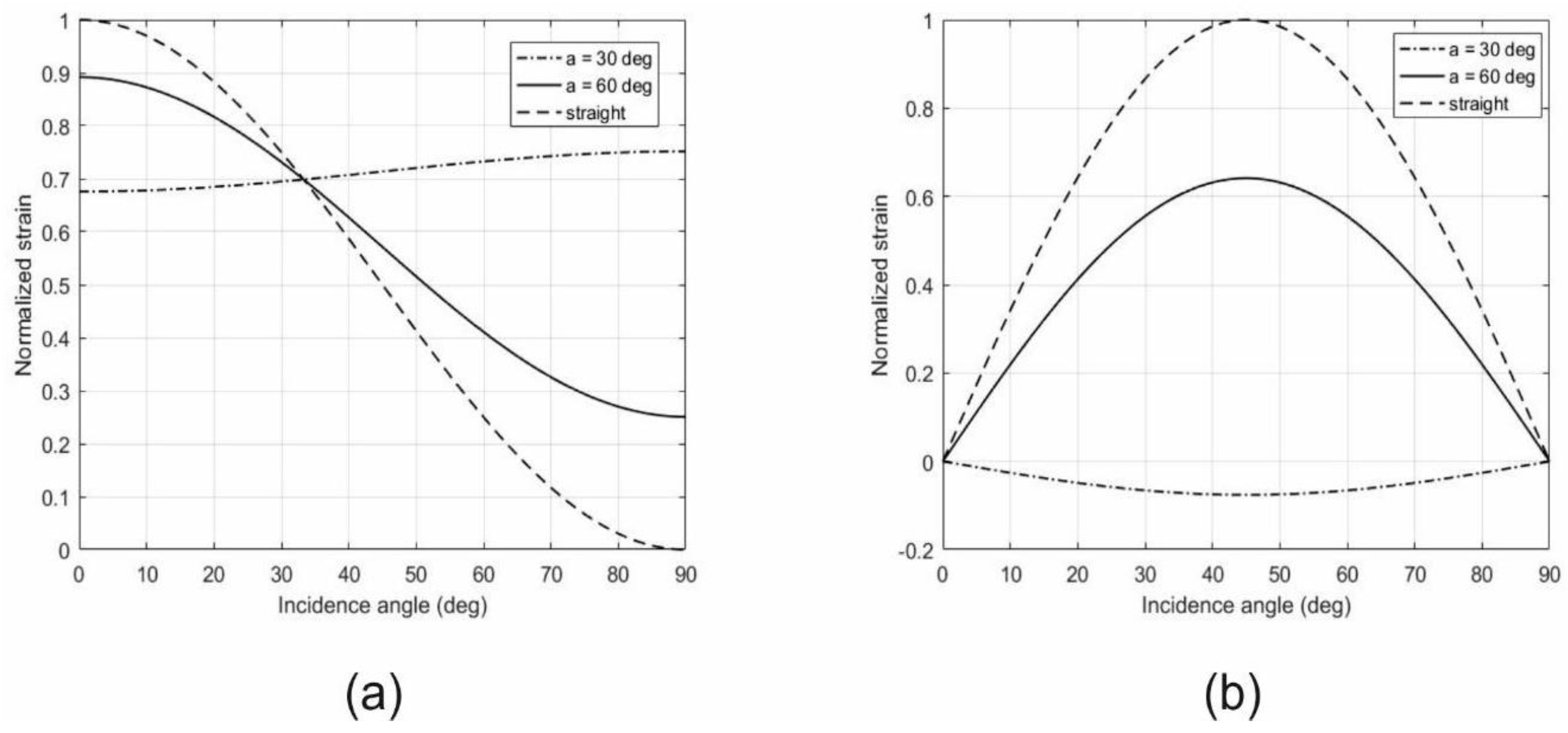
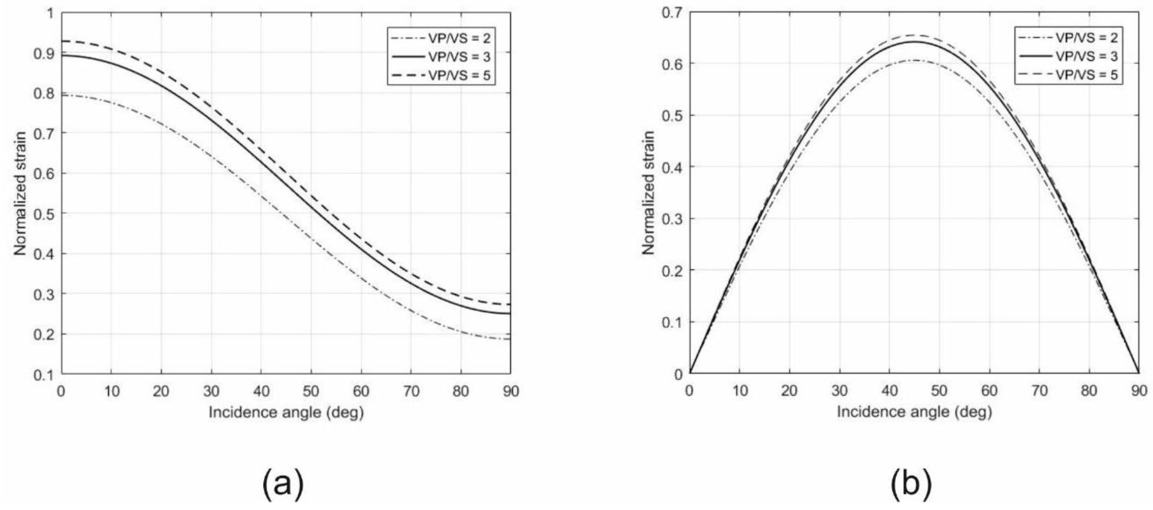
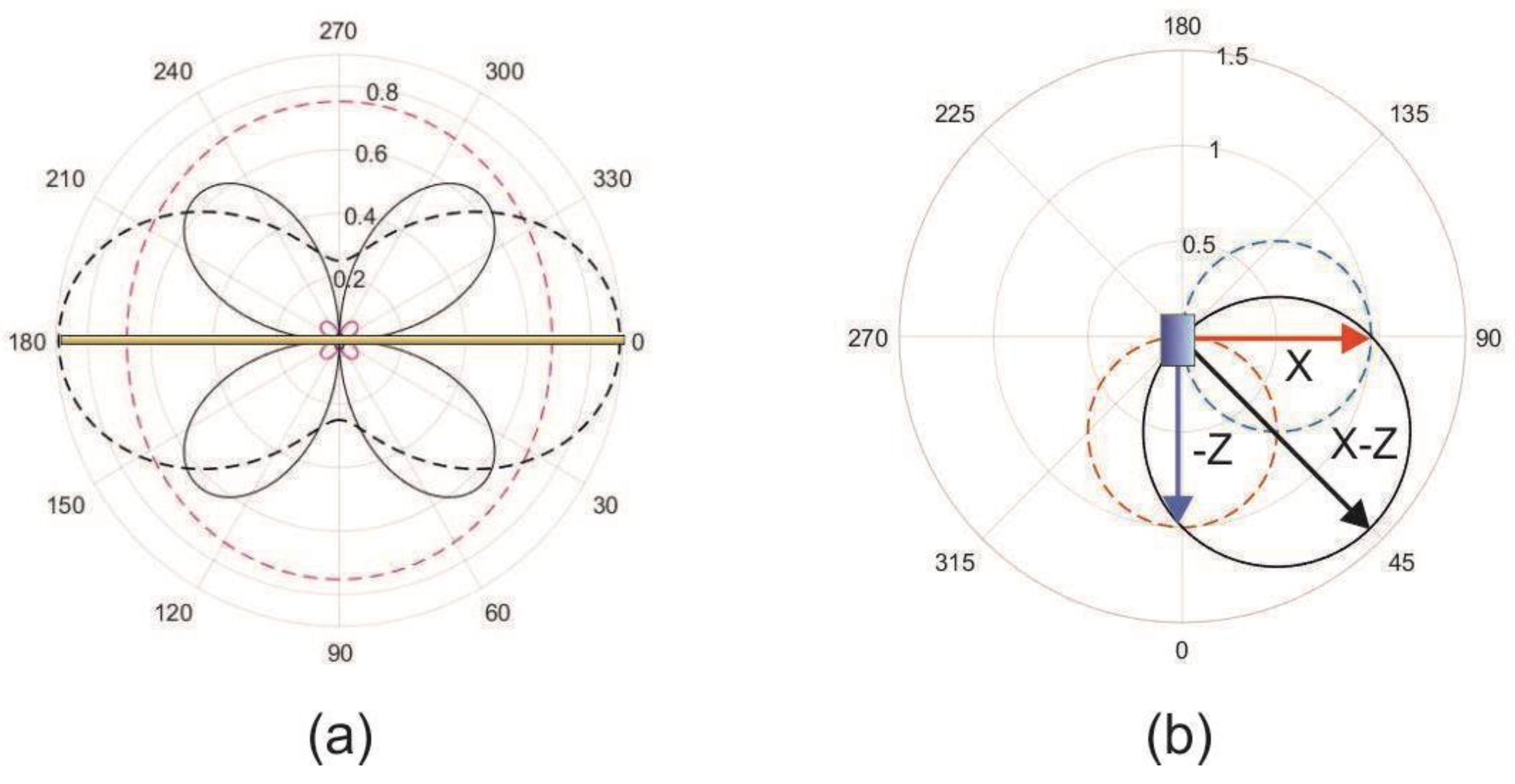
2.1. DAS Fibers Sensitivity

A standard straight fiber has its highest sensitivity to P-waves when the angle of incidence ϑ of the wave is 0 degrees; it decreases as cos²(ϑ) as the angle of incidence increases, reaching its minimum when the wave propagation is orthogonal to the fiber [27]. The broadside sensitivity of HWC is instead flatter with the angle of incidence of a P-wave [28,29] (Figure 1a), depending on the wrapping angle, i.e., the angle between the wound fiber axis and the plane normal to the cable axis. Conversely, the HWC sensitivity response to S-waves is variable with the wave impact angle as sin2ϑ. It is maximum at incidence angles of 45 degrees, and it is zero at 0 and 90 degrees [28]. Figure 1 shows the theoretical curves calculated for a fiber with wrapping angles of 60 degrees (used for this survey) and, for a comparison with results shown in literature, 30 degrees, perfectly coupled without sliding (modified after Kuvshinov [28]). These curves change in function of the cable and formation properties, which, in this example, are V_P = 1500 m/s, density ρ = 1600 kg/m³, and V_P/V_S = 3, while the fiber properties are those used by Kuvshinov [28]. The bold line in Figure 1a is the normalized strain sensitivity to P-waves obtained with a wrapping angle of 60 degrees, plotted vs. wave incidence angle. The dashed line is the sensitivity of a linear DAS cable, i.e., with a wrapping angle of 90 degrees, to P-waves. The dashed–dotted curves correspond to a wrapping angle of 30 degrees. Figure 1b shows the corresponding sensitivity curves to S-waves. Note that the maximum magnitude of their response is at 45 degrees for all the curves. The examples shown in Figure 2 show that the responses are sensitive to V_P/V_S, in this case, with a wrapping angle of 60 degrees and different values of V_P/V_S. These curves do not include gauge-length effects. The gauge length adopted by the fiber to record the seismic data acts as a spatial filter, with effects on the sensitivity of the fiber depending on the signal wavenumber, and, in turn, on the incidence angle for a wave with a given signal frequency [30]. Local responses, such as coupling and local near-surface inhomogeneities with effects for an HWC fiber-optic cable buried in a trench dug ad hoc, can influence the results.

Conversely, the P-wave sensitivity response for a vertical geophone is cos(ϑ). The basic difference between the DAS and geophone transducers is that the native output signals of the DAS cable and of the geophones are obtained from measurements of different physical quantities, usually strain rate and particle velocity, respectively. In view of their responses, the HWC DAS cable offers the advantage of using large broadside receiver arrays at the surface [31].

From a conceptual point of view, in Figure 3a, we represent in polar coordinates the sensitivity results shown in Figure 2a,b. The sensitivity curves are calculated with the parameters of the examples shown in Figure 2, using the results obtained with wrapping angles of 60 and, for comparison, 30 degrees and V_P/V_S = 3. The angle of the polar representation is the incidence angle of the wave relative to the fiber cable, horizontal in Figure 3. The angle of 0 degrees means coaxial, while 90 degrees means orthogonal to the cable. With the adopted parameters, the variation in the sensitivity to P-waves (dashed lines) is low for a wrapping angle of 30 degrees (purple line) and the broadside variable with a wrapping angle of 60 degrees (black line). The sensitivity changes for variations in V_P/V_S. Conversely, the sensitivity to S-waves (bold lines) has prominent lobes with their maxima for example at 45 degrees and −45 degrees (315 degrees), with different amplitude for wrapping angles of 60 and 30 degrees. This means that the HWC fiber enhances shear events with intermediate inclinations between those of the vertical Z and horizontal in line X geophone components. As discussed earlier, these polar sensitivity responses do not include directional effects introduced by the gauge length, which reinforces signals with vertical travel paths normal to the fiber.

The HWC fiber does not separately record the Z and X events. However, they are available in the geophone data. Their combination can be used to steer the signal components pointing the sensitivity to desired directions, 45 and −45 degrees (Figure 3b). In Figure 3b, the 0 degrees for the incidence angle corresponds to the −Z component direction (blue vector). Its sensitivity to S-waves is sin(θ) (blue dashed lobe). The 90-degree angle corresponds to the X component direction (red vector). Its sensitivity to S-waves is cos(θ) (red dashed lobe). Using a linear combination of X and Z, we simply rotate the lobes, pointing to the desired direction. This is a linear combination of geophone components, and the shape of its lobe does not change, it only rotates. In other words, we point to the same sensitivity lobe direction with HWC DAS and geophone signal combination, but with different shapes, as can be expected for a comparison of geophones and a strain-rate transducer. Obviously, a refined steering of the pointing vectors by a weighted combination of the field signals would benefit from the processing of the wavefields with an evaluation of the paths of the emerging rays in the seismic model, not included at this stage of the analysis. Conversely, the sensitivity response to P-waves is flatter in the HWC DAS data, as shown in Figure 3a, dashed line. These results are calculated in an unbounded medium. With measurements at the shallow surface, the presence of Rayleigh waves should also be considered.

2.2. Feasibility Study

The Hellisheiði geothermal field (Figure 4) is situated in the southern part of the Hengill volcanic system, near Reykjavik, Iceland. This area lies at the intersection of the Reykjanes Volcanic Belt, the Western Volcanic Zone, and the South Iceland Seismic Zone, which contributes to its complex geological structure. The Hengill system is characterized by a central volcano and a fissure swarm with a graben structure. The bedrock predominantly consists of hyaloclastite, including tuffs, breccias, and pillow lavas formed during glacial periods, along with intrusive rocks and lavas from interglacial periods. Tholeiitic basalt is the main magma type, but more silicic rocks are also present, particularly in the central volcano. The geothermal field itself reaches temperatures above 300 °C at a depth of 1000 m below sea level [32], making it one of Iceland’s largest and most productive geothermal areas.

The need for a feasibility study arose from geophysical characterization aspects and operational reasons. The absence of borehole seismic data in the reservoir wells and of a reliable preliminary seismic model demanded efforts to define the basic starting model for the analysis. The proper use of the novel E-Vibe and the broadside sensitivity HWC DAS with the available project resources required the evaluation of the expected wavefields in the 2D seismic data and of the reservoir illumination conditions. The numerical simulation of the active seismic wavefields provided information useful to determine the acquisition parameters (e.g., source geometry, spatial sampling, etc.), as well as data useful for signal recognition during the in-field Quality Control (QC) in this complex area. The numerical simulation also provided synthetic data for full-waveform analysis after acquisition, to support the wavefield interpretation as a starting point of the seismic processing. Because at the initial stage of the project, the available seismic-model information was poor, for the acquisition planning we computed synthetic 2D elastic propagation using the geological model (provided by TU Delft) along a section approximately orthogonal to the main seismic acquisition line, from which we extracted a model (Figure 5) including the seismic acquisition area (Figure 4). This reduction was performed to better fit the available computational resources and resolution requirements.

In fact, in this preliminary phase, we were interested in understanding the seismic response in this area, and the orthogonal model (the only one available at that moment) suited the purpose well enough. We assigned compressional wave velocity (V_P) and density to each individuated lithological layer (Figure 6), using initially averaged values derived from the literature according to their depth [33,34,35]. Then, we adjusted the P-wave model according to laboratory analysis results. The corresponding shear-wave velocity model was computed from the V_P model using the ratio V_P/V_S = 1.8. This averaged estimation was derived from the 1D compressional- and shear-wave velocity profiles calculated during the COntrol SEISmicity and Manage Induced earthQuakes (COSEISMIQ) Project [35].

The P-waves seismic model along the line is reported in Figure 6 and it points out the different velocities of the basaltic layers.

We used this model to evaluate the variations in the P-waves and S-waves sensitivity responses, analytically represented in Figure 2, keeping into account the shallow seismic properties along the main seismic line [23].

2.3. Synthetic Seismograms

Synthetic seismograms were calculated for the active seismic data using a point force and geophone receivers, and simulated pressure signals. A staggered grid finite-difference elastic 2D propagation code was used to compute the synthetic seismograms using the seismic model shown in Figure 6. This model was discretized for different tests with squared pixels of 5 m, 2 m, and 1 m sided to properly analyze the response and the frequency content of the simulated signals. Common-source seismograms were generated by a full-waveform elastic simulation of the 2D wavefields emitted by the source at the central position in the model. We calculated the results with different discretization, using 2 m × 2 m, and 1 m × 1 m grids. The source was a Ricker wavelet with peak frequencies of 25 Hz and 40 Hz, respectively. The source mechanism was applied both as a vertical force and a horizontal force. Nevertheless, in the field acquisition, we used only the vertical source mode, invoking reciprocity common-source results obtained by a vertical source, and horizontal receiver components can be interpreted as common receiver gathers obtained with horizontal sources and a vertical receiver. With these source configurations, we recorded both the vertical and the horizontal components of the receivers (particle velocity, thus providing geophone signals). Moreover, using the V_s velocity model, we calculated acoustic seismograms by a pressure source and pressure receivers to simulate the SH wavefields, thus avoiding P–S-wave conversions in the results. The choice of recording both the vertical and horizontal synthetic components, in addition to enabling a better characterization of directional events recorded by geophone signals, is even more important because the broadside HWC DAS deployed at the surface is sensitive to vertical and horizontal in-line waves [28,29] (Figure 1 and Figure 2). The horizontal line-orthogonal components were also included in the study to detect the possible presence of SH waves.

Sample shots calculated using the model discretization grid 2 m × 2 m and a source peak frequency of 25 Hz are shown in Figure 7 for different types of sources and receiver components. The data simulations showed that different events can be potentially interpreted for the relevant markers, which are basalt and hyaloclastite formations, with differences in the wavefields due to their radiation conditions and nature: P-wave arrivals and reflections, S-wave (SV) arrivals and reflections, converted P–S and S–P-waves. In Figure 7a–c, we can observe the apex of the P-wave reflection from the uppermost interface between basalt and hyaloclastite at about 200 ms in the near-offset traces. We also interpret the P-wave reflection interface between the deeper basaltic layer and hyaloclastite at about 500 ms. In the near-offset traces, the P-wave reflection from the shallower hyaloclastite and basalt interferes with the first S-wave reflection at about 360 ms. The S-wave reflections are clearly visible in the uncoupled S-wave propagation shown in Figure 7d. The P-wave reflection from the deepest basaltic layer, expected near the source at about 820 ms, is better visible in the vertical-receiver component (Figure 7a,c). The investigation of these wavefields will be the object of future processing. This kind of analysis is important for signal recognition in field data.

We calculated the synthetic data with different trace interspacing, according to the grid used to discretize the model. Reflection seismic data are generally of poor quality in volcanic environments because of diffraction and scattering, attenuation, and static problems [26]. To overcome this problem, we ran simulations of array patterns that can be used to boost reflections and improve the S/N in the real data. The steering of the arrays makes it possible to steer the directivity of the patterns, which in this phase was mainly used to reinforce the reflection arrivals with vertical travel paths. The acquisition receiver-array pattern can be effectively simulated with synthetic data calculated with refined grids and with real data, thanks to the DAS dense spatial sampling. Figure 8a shows the synthetic signal (vertical component) by a punctual single-trace (2 m) representation, and Figure 8b shows the simulated horizontal surface-receiver arrays (each trace was obtained with a pattern of 50 m), for a vertical force source. This type of array-pattern simulation has been successfully used in the processing of the seismic sections of the real data [23].

Even if not all these calculated components were used during the early interpretation phase, and despite the provisional nature of the seismic model because of the limited knowledge of the seismic properties before acquisition, the synthetic seismic results provided confirmations for the capability of the subsequent acquisition campaign to detect signals useful for the reservoir monitoring, in terms of signal arrival times, event shapes, and interference of wavefield components.

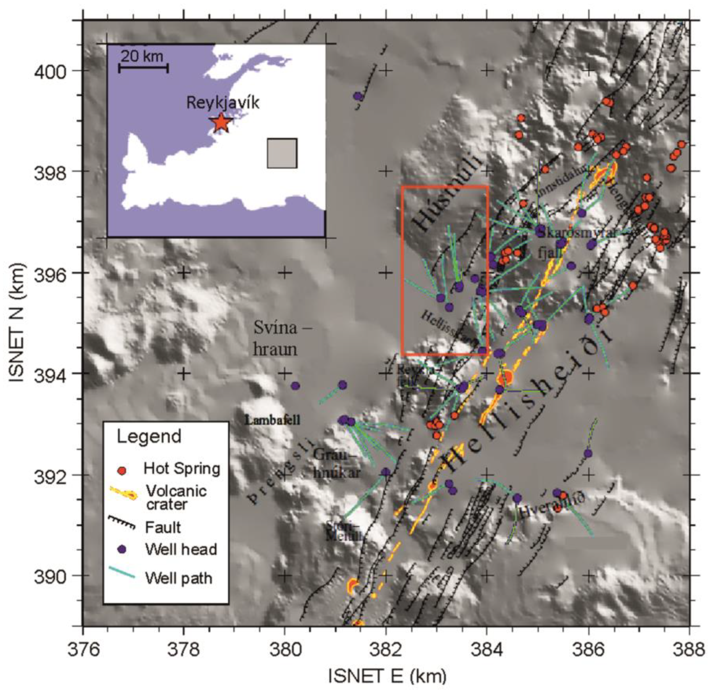
2.4. Seismic Acquisition at Hellisheiði Geothermal Field

The acquisition control was carried out both on-site and in the office, via remote connection. The area investigated in this study covers the surface projection of a fault, identified near the OR-Reykjavìk Energy Geothermal Plant located in Hellisheiði. The shallow and deep targets of the survey are located at approximately 0.7 km and from 2 km depth below the surface. The design of the receivers and sources acquisition lines was prepared considering the complex surface logistics, topographic, and access conditions of the area.

The active source used for the survey was the STORM-10, an electromagnetic seismic vibrator (E-Vibe) developed by Seismic Mechatronics. Although this source can be re-configured from the vertical vibration mode to the horizontal vibration mode, during the survey the vibrator was operated only in the vertical mode. The vibration points (VP) (with positions indicated by white circles on the map of Figure 9) closely follow the path of an approximately 2 km long trenched linear tactical (conventional) and HWC DAS line installed by Silixa for passive- and active-monitoring purposes [20]. The line of the vibration points was extended at the ends of the line where the topographic conditions allowed. This solution was adopted to increase as much as possible the coverage of the recordings and the fold in the final stacked sections. The HWC type of DAS cable was chosen because of its broadside sensitivity, suited for detection of wave fields emerging from deep structures [31]. At the same time, the active data obtained with this setting were used also to analyze the properties of the shallow layers by inversion of the first arrivals [23]. The results were then utilized to update the estimation of the formation properties.

2.5. Receiver Line Configuration and Data Merging

Figure 9 shows the map of the multi-tool experiment during the baseline active-source seismic campaign at Hellisheiði. The acquisition layout of the seismic receivers consisted of the HWC DAS line, with about a 1.5 km long active trenched HWC recording section, with approximately 1 m receiver spacing and 10 m gauge length [20]. The HWC cable pitch angle is 30 degrees, corresponding to a 60-degree wrapping angle, the cable diameter is 25 mm, and the depth of the trench is around 0.5 m. The natural frequency of the DAS system ranges between 0.001 Hz and 50 kHz. The DAS data were recorded with a 1000 Hz sampling frequency and 20 s recording length for the individual seismic records. In addition to the HWC DAS section, a conventional (tactical) DAS cable approximately 350 m long ran from the HWC section to the fiber-optic DAS interrogator unit.

Figure 9. Map showing the experiment layout, in which different acquisition systems were used, including fiber-optic HWC DAS and tactical cable, 2C GEODE, and 3C SOLO geophones co-located along the main (HWC) line (IN-line); the SOLO geophones were also disposed along a perpendicular (yellow dots) line (X-line). The source positions are marked with white bullets. The arrow at the bottom indicates the North.

Figure 9. Map showing the experiment layout, in which different acquisition systems were used, including fiber-optic HWC DAS and tactical cable, 2C GEODE, and 3C SOLO geophones co-located along the main (HWC) line (IN-line); the SOLO geophones were also disposed along a perpendicular (yellow dots) line (X-line). The source positions are marked with white bullets. The arrow at the bottom indicates the North.

Along the HWC DAS line, a total of 48 2-C, 4.5 Hz geophones (TUD geophones of a GEODE system), for a total line-section length of 470 m, were deployed with 10 m spacing for the detection of P and SV waves, i.e., with the horizontal axis of the sensor oriented in-line. The TUD field data were recorded with a sampling frequency of 500 Hz and 20 s recording length.

To cover all the HWC line, a total of 92 3-C, 5 Hz SmartSolo^® remote geophone stations (from here on denoted as SOLO) were deployed with 20 m spacing, in the proximity and along the HWC DAS line. Another line of 56 3-C SOLO units was deployed along a cross-line (also indicated as x-line), with the same receiver spacing (20 m). Their sampling frequency was 1000 Hz and the recording length was 20 s.

The role of the SOLO and the TUD geophones was to compare and validate the results obtained by the HWC DAS line during the baseline survey and, in view of the different responses and nature of the recorded signals, to analyze the different wavefields contained in the strain-rate and particle-velocity output signals recorded by the DAS and the geophone components, respectively, and using different layouts.

Because of the considerable amount of data produced by the DAS system, and the consequently long conversion time required to retrieve and uniform the formats of all the records, we developed a multi-tool approach and dedicated custom-made software. This tool was effectively used to enhance the monitoring and QC, and to enable a detailed comparative signal analysis and a nearly real-time data interpretation with remote assistance from headquarters. The daily data output was one standard SEGY file with the collection of all the daily records, including the E-Vibe pilot signals, recorded with a sampling frequency of 4000 Hz and a 15 s sweeping line. Only the DAS and GEODE geophone data, together with the source pilot signals, were available for continuous QC purposes during the acquisition. Conversely, the data from the remote SOLO geophone stations were retrieved, and downloaded from the station’s memory, re-formatted, and analyzed only after the end of the survey. At the end of the merging procedure, for each shot, all the recorded traces were re-sampled with the same 1 ms sampling interval, and gathered into a single field record, to facilitate QC with data comparison and joint processing of traces obtained from different systems.

2.6. Vibrator-Source Parameters with Focus on the Pilot Signal

The active source used for this survey is the electromagnetic vibrating seismic source (E-Vibe) recently developed by Seismic Mechatronics, specifically designed and adapted for the SUCCEED project. The vibrating mass is entirely mounted, together with its power and control electronics, on a robust telehandler, capable of accessing in the difficult terrain nearly all the designated VPs (Figure 10). The seismic source was operated in the vertical-vibration mode, i.e., with the mass vibrated vertically.

With respect to the expected source radiation properties (apart from possible SH effects produced by lateral inhomogeneities), the vibration source operated in the vertical mode radiating P- and SV-waves, as well as converted PS- and SP-waves in the signals recorded with offset. All these aspects were considered in the planning and preparation of the field demonstration phase.

The total number of VPs was 59, including a few shot points energized at the ends and of the crossing line to obtain common-shot data with reciprocal geometry. One relevant aspect is the high repeatability of the E-Vibe source, tested in this semi-continuous acquisition experiment. Besides the analytic (synthetic) signal provided by the Vibrator control system, we recorded and used acceleration components of the baseplate and vibrating mass that allowed us to estimate ground force (Figure 11) and we used it as a reference signal for correlation as well [36]. Figure 12 shows the Fourier frequency spectra of the reference and ground-force signals.

A signal processing analysis was performed to investigate the penetration range of the recording system in the area. Consistent DAS results were obtained with geophone and fiber-optic data. These receiver tools record in different frequency ranges, and the vibrator source is able to produce signals starting from a few Hz up to 250 Hz.

The first configuration of the source parameters was set with higher emission frequencies in the initial tuning phase. However, the analysis of the signal content during the ongoing survey, given the survey target and the operational resources, suggested a reducing the maximum frequency for the subsequent survey production phase. In the initial testing phase, we used the following source parameters: sweep type upsweep, sweep length 15 s, and frequency range 2–240 Hz. The driving force was set to 2100 lbf, i.e., 93% of the maximum peak force of 2250 lbf of the source, in order to operate the device with a safe margin of tolerance for a high number of repetitions. The tests took place on three different shot points, to evaluate the S/N as the number of repetitions increases up to more than 30. From these tests, we observed a plateau of the S/N after stacking 16 records.

In the production stage, we adjusted the sweep frequency range to 2–150 Hz in order to improve the depth penetration. The source spacing during production was 40 m acquiring 16 records per VP position.

In the early pilot correlation tests, we used both the external synthetic reference sweep (Figure 11, trace 6) and the ground force (Figure 11 trace 7) calculated by a weighted sum of the reaction mass and baseplate signals [36] as the pilot signals for the correlation with the seismic signals. The ground force was used to take into account the variations in the seismic signals obtained with the VPs along the vibration path. Assuming that the signature of the radiated signals from a vertical force is the time derivative of the ground force [37], we used the following approximated approach. We express the pilot signal by iωP(ω)e^iφ in the Fourier frequency domain, where P and φ are the amplitude and the phase spectra (we omit for convenience the frequency–time dependency). To avoid instabilities in the results, instead of deconvolving the seismic signals by the time derivative of the estimated ground force, we cross-correlated the seismic signals using the ground force P(ω)e^iφ. Then, we time-integrated the ground force cross-correlation result by –iω. The difference with deconvolution is that with this approach, we obtain the estimation of the signal power spectrum as P_e(ω)P(ω), where P_e(ω) is the effective ground force signal, instead of using P_e(ω)/P(ω) ≃ 1, while the phase difference is the same in the correlated and deconvolved results. The choice of this approach was based on the observation that the amplitude spectra of the calculated ground force are reasonably flat (Figure 12d). The cross-correlation results obtained with the ground force and with the synthetic sweep for a selected shot recorded by the geophones of the cross-line are compared in Figure 13.

3. Results and Discussion

3.1. In-Field and Remote QC from Headquarters

The project team provided both in-field and remote (at Headquarters) support during the test and acquisition phases, with prompt technical assistance to speed up the collection of records during the early QC test phase. The remote QC was performed in near-real time; i.e., the relevant time to make prompt decisions on acquisition parameters (to optimize the use of the resources and the acquisition quality). The main target of the QC was to optimize the acquisition parameters for the assessment of the desired penetration and resolution for the reservoir characterization, in consideration of the in-field response and of the operational resources available for the field campaign. The initial QC determined the choice of vibration parameters, energization interval, number of records in the stacks, sweep mode, frequencies, and length. The acquisition was tuned during the survey, based on sweep and seismic signal sample tests, after the initial tests performed at the beginning of the survey for the assessment of the optimal S/N in the data. For this purpose, the pilot traces were recorded shot-by-shot by the source unit. The pilot signals were made available at the end of each day in SEGY format. Essential for the QC was the merging, formatting, and editing of the different datasets with the same recording parameters (20 s record length, 1 ms sampling interval), to be usable in a relevant time during acquisition. Examples of field-QC on common-shot gathers obtained with the same source are shown in Figure 14, where we compare the results obtained by the TUD, SOLO, and HWC receivers located in a common line interval. The higher spatial sampling of HWC signals is evident in Figure 14c, resulting in a higher spatial resolution.

3.2. Post-Acquisition Signal Analysis

All the data, including the SOLO signals, were available for the deferred signal-analysis stage. Advanced steps of pre-processing were applied to the datasets at the headquarters, with formatting and editing of the complete active-source seismic dataset, including positioning of the receiver traces of the different systems. Further processing was performed on the complete dataset [23], and is currently ongoing with the aim of improving the S/N in the data, and evaluating the seismic wavefields. Particular attention is given to the characterization of the DAS signals and of the source emission, by analyzing and processing the seismic wavefields in the different recordings to produce reliable subsurface images of the reservoir zone of interest. The wavefield processing steps included seismic signal analysis with the support of synthetic modeling, multi-component and S/N analysis, multichannel data processing to investigate deep structures, and analysis of the source performance and the depth of penetration, while further analysis will include imaging by seismic-interferometry approaches.

3.3. S/N Improvement in the Optical Signals

From the preliminary analysis during the QC phase of raw and cross-correlated data emerged the presence of some optical noise in the recorded signals. This noise, known as common mode noise (CMN) and sometimes called horizontal noise [27], consisted of time-aligned events, which affect the variable extents of the results obtained from both uncorrelated and correlated data. This noise is caused by sound entering the DAS interrogator and contaminating all channels of the recorded seismic data with an identical set of noise. All possible precautions must be implemented to reduce the CMN, such as using anti-vibration tables placed under the interrogator.

For the S/N analysis, the availability of the non-stacked individual records was important since it allowed the selection and editing of the noisy field records. For this purpose, we applied noise estimation and reduction procedures based on aligned noise recognition algorithms developed ad hoc, as discussed in subsequent works [23]. Figure 15 shows the effectiveness of the adopted noise reduction approach on a stacked common-shot gather cross-correlated using the ground-force signal. This preprocessing analysis was then applied to all the HWC DAS data.

Figure 15. (a) HWC DAS cross-correlated common-source record before CMN optical-noise removal. (b) DAS HWC common-source record after CMN optical-noise removal. In (b) the S/N is significantly improved. The cross-correlated signals are obtained using the ground-force pilot.

Figure 15. (a) HWC DAS cross-correlated common-source record before CMN optical-noise removal. (b) DAS HWC common-source record after CMN optical-noise removal. In (b) the S/N is significantly improved. The cross-correlated signals are obtained using the ground-force pilot.

3.4. Tuning of the Synthetic Model by Field Results

The seismic model used in the feasibility study was then modified, and periodically updated using new available information, to match with the subsurface structure under the main HWC line; this updated model is described in detail in the processing study reported by Bellezza et al. [23]. Numerical simulations were then calculated to compare the synthetic and field data wavefields. Using the preliminary results of the baseline active seismic campaign (see also Bellezza et al. [23]), we performed a calibration of the seismic model with a revision of the velocity profiles. These data were used for QC of the acquired data after the acquisition. Synthetic seismograms of the vertical (Z) and horizontal in-line (X) components were calculated with a 2D finite-difference elastic code (modified after Levander [38]). The model grid was discretized using 1 m × 1 m pixels. The source is a vertical force, according to the vibration mode of the field source.

We used a Ricker wavelet with 20 Hz peak frequency, and P-wave velocity derived from the laboratory measurements [22], an average V_P/V_S ratio of 1.8, and Gardner’s relation [39] to calculate the formation density. Figure 16 shows the horizontal receiver components in (a) synthetic and (b) SOLO field data, which highlights similar trends for the observable events, confirming that the model fits the data quite well.

3.5. Analysis of HWC DAS and Multi-Component Geophone Signals

Deferred processing was performed at the Headquarters to analyze the signal wavefields from the three recording systems. We jointly analyzed the wavefields in the multicomponent geophone data deployed along the main HWC line and in the single-output trace of the broadside HWC DAS signals. The results of the TUD and SOLO geophone systems are consistent, despite their different responses and spatial sampling along the receiver line. Figure 17 compares the signals of the TUD geophone components with the HWC signals recorded along an interval of approximately 400 m, where these co-located data are available. Figure 17a,b show the TUD vertical and TUD horizontal (in line) components, respectively. Figure 17c shows the HWC DAS signal. The CMN optical noise in the HWC DAS data was removed by pre-processing (Figure 17c).

After S/N improvement, the HWC signal is clearly interpretable at the larger offset distances from the source vibration point (VP), with S/N comparable to that of the geophone results. We may observe that in these results there are correspondences and differences, as can be expected from measurements of different physical quantities (strain rate and particle velocity) and using different components, i.e., one receiver component vs. two components for signal comparison. Similar events can be interpreted, however, with different distributions in the different wavefields. Moreover, different sensitivity responses are expected for these signals, as discussed in the introduction of this paper. The result highlights the consistency of the signals between the different types of sensors and better continuity of the HWC DAS than TUD geophones. To better characterize the investigated wavefields, we extend the analysis to the entire main seismic line; for a comparison between the HWC and geophone signals along the main line, we used the SOLO components, although these receivers are less densely sampled in space than the TUD ones, since the TUD line does not cover the complete extension of the main HWC line.

Based on considerations made in Section 2.1, in order to compare the HWC and SOLO geophone signals in field data and focusing on the S-wave components, we calculated as a first approximated approach the bulk Z ± X using the SOLO geophone components of the field data. In view of the different nature of the recorded signals and the different trace spacing used for the geophone and optical lines, the agreement of the wavefield’s trends in the results shown in Figure 18 appears interesting and encouraging for the wavefield interpretation. We can observe that the Z-X combination, still with differences, better matches the HWC signals, more than the separated individual components, as with the TUD data (Figure 17). Further analysis with the comparison of the stacked sections of the SOLO and HWC data obtained with the same model and processing parameters, but with different spatial sampling, are discussed by Bellezza et al. [23]. They evaluated a comparison with passive seismic results using the DAS lines by Stork et al. [24] and HWC lines compared to SOLO [25].

This provisional example shows interesting corresponding events in the geophone and fiber-optic data, validating the effectiveness of the HWC DAS, which has been the unique sensor type used for monitoring in the planned time-lapse survey and for depth imaging.

3.6. Source Penetration

The E-Vibe source penetration in the context of the survey was estimated during the project, using seismic section results obtained in the deferred phase after the initial QC. Figure 19 shows details of an HWC DAS seismic section obtained during the deferred seismic processing phase [15].

In this complex volcanic area, we observe events at two-way times (TWTs) of 1.5 s and more. The corresponding depth, assuming a P-wave average velocity of 3500 m/s from the stacking interval velocity functions, is of the order of more than 2600 m, which includes the monitored reservoir.

The part of the seismic section shown in Figure 19 only serves to illustrate the penetration of the source, while the analysis and interpretation of the entire seismic section are discussed in detail in Bellezza et al. [23], where the horizons are interpreted.

3.7. Considerations on Mathematical Optimization Frameworks for Survey Design

The 2D seismic survey described in this work was constrained about the path (spatial position) the different sensors could occupy, which was related to the logistics and accessibility. The parameters we could optimize were those linked to the source (sweep, number of VPs, VPs per position, etc.) and the spatial density of the sensors. The use of HWC DAS in seismic acquisition allows a huge number of channels at a relatively low cost compared to traditional sensors, especially for deployment on long arrays. Recently, some authors faced the general issue of enhancing the seismic acquisition design by considering some mathematical optimization frameworks for optimal survey design with traditional sensors. Zhang et al. [40] showed how techniques from graph theory can be used to optimize acquisition geometries for low-cost sparse 4D seismic, a fundamental aspect of modern-day reservoir management and monitoring of geological carbon storage, which requires costly time-lapse seismic data collection. Guo et al. [41] stated that seismic acquisition costs are directly associated with the number of sensors used in the survey. Limiting the number of sensors in a seismic survey can be beneficial, especially when sensors are expensive to purchase, deploy, and maintain. Their work explores an optimal design method for ocean bottom node (OBN) detector deployment, based on a reinforcement learning (RL) approach. Kumar et al. [42] observed that full-waveform inversion (FWI) has delivered significant improvements in velocity and image quality but can be compromised due to the acquisition parameters and associated costs required to optimize FWI. To reduce the acquisition cost, simultaneous acquisition is preferable, which requires a source separation framework. The authors propose generating an optimal survey design using the spectral-gap-based rank minimization, termed as generalized survey optimization with constraints. The proposed technique is computationally efficient and uses realistic environmental and instrumental constraints to generate source and/or receiver locations, where the acquisition is constrained with random time dithers.

The previously described studies confirmed how the optimization of seismic surveys will become even more important as the monitoring applications for CO₂ and energy storage are increasingly requested in the efforts of global decarbonization. In this framework, the use of DAS turns out to be a cost-effective solution.

4. Conclusions

In this work, a feasibility study and data acquisition of an active seismic survey in a geothermal site by means of a multi-tool approach has been described, including numerical analysis, quality control, and preliminary pre-processing steps. The baseline active seismic monitoring was completed in July 2021 at the Hellisheiði geothermal field site, where brine and CO₂ were injected for performance enhancement of the power plant. The acquisition layout was designed and planned to accomplish site characterization and monitoring by means of helically wound cables (HWC), distributed acoustic sensing (DAS) cables, and auxiliary surface geophones, along with an innovative continuous electromagnetic E-Vibe source. The fiber-optic HWC DAS cable was selected for its broadside sensitivity, to record up-going signals coming from deep reflectors, the target of the monitoring. The active source E-Vibe vibrator acquisition was operated in the vertical-vibration mode along the same line path as the HWC DAS sensors. The analytic study about fiber sensitivity provided a deeper understanding of the expected wavefields recorded during the acquisition compared to the wavefields collected by the geophones, which record separate components of a specific wavefield. Synthetic seismograms modeled by means of finite-difference 2D propagation codes were successfully used to simulate the wavefields expected in real data and to support wavefield analysis and interpretation. In-field and remote quality control of data enabled the acquisition parameters to be optimized, while deferred signal analysis allowed the complete seismic dataset to be inspected. The benchmark of broadside HWC DAS cable and TUD GEODE/SmartSolo^® geophones responses pointed out comparable results in terms of sensitivity and a good kinematic match of the different seismic phases. A drawback of the HWC DAS is the common mode noise, which is caused by sound entering the DAS interrogator and contaminating all channels of the recorded seismic data with an identical set of noise. This noise masks the signal and must be removed or at least attenuated before the processing phase with an ad hoc procedure. Moreover, the HWC fiber does not record separately the vertical and horizontal components of the wavefields, and this could affect the wavefield recognition compared to 3C geophone data. Given the low quality of the collected data, conducting the analysis of the different wavefields was not trivial (highlighting the challenges of the applied approach); so, from this point of view, seismic modeling takes on even more importance in the analysis of the data. In non-volcanic environments, in general, more suitable for seismic methods, we expect the quality of the HWC DAS data to be improved. Despite the previously described issues that must be dealt with, the use of fiber-optic sensors highlighted the advantage of providing, besides permanent installations of easy deployment, a dense array of receivers, regularly spaced in this survey with inter-trace distance of approximately 1 m, which is particularly suited for monitoring purposes; moreover, the high spatial sampling allows the simulation of array patterns that can be used to boost reflections and improve the S/N in the real data. The preliminary comparative analysis among signals of these different types of sensors confirmed that an HWC DAS cable can be used to effectively image the subsurface in active seismic surveys also combined with an environmentally friendly electromagnetic source. Overall, this experimental work represents a unique case of a joint and comparative signal analysis of detected wavefields recorded by different sensors in high-temperature complex geothermal areas, and it highlights the feasibility of this approach for characterization and monitoring of subsurface, for instance, in the frame of energy and CO₂ storage, and also from a time-lapse monitoring perspective.

References

1. Tomassi, A.; Caforio, A.; Romano, E.; Lamponi, E.; Pollini, A. The development of a Competence Framework for Environmental Education complying with the European Qualifications Framework and the European Green Deal. J. Environ. Educ. 2024, 55, 153–179. [Google Scholar] [CrossRef]
2. Lindsey, N.J.; Martin, E.R.; Dreger, D.S.; Freifeld, B.; Cole, S.; James, S.R.; Biondi, B.L.; Ajo-Franklin, J.B. Fiber-Optic Network Observations of Earthquake Wavefields. Geophys. Res. Lett. 2017, 44, 11792–11799. [Google Scholar] [CrossRef]
3. Walter, F.; Gräff, D.; Lindner, F.; Paitz, P.; Köpfli, M.; Chmiel, M.; Fichtner, A. Distributed acoustic sensing of microseismic sources and wave propagation in glaciated terrain. Nat. Commun. 2020, 11, 2436. [Google Scholar] [CrossRef] [PubMed]
4. Lellouch, A.; Schultz, R.; Lindsey, N.J.; Biondi, B.L.; Ellsworth, W.L. Low-Magnitude Seismicity With a Downhole Distributed Acoustic Sensing Array—Examples From the FORGE Geothermal Experiment. J. Geophys. Res. Solid Earth 2021, 126, e2020JB020462. [Google Scholar] [CrossRef]
5. Sladen, A.; Rivet, D.; Ampuero, J.P.; De Barros, L.; Hello, Y.; Calbris, G.; Lamare, P. Distributed sensing of earthquakes and ocean-solid Earth interactions on seafloor telecom cables. Nat. Commun. 2019, 10, 5777. [Google Scholar] [CrossRef]
6. Lellouch, A.; Yuan, S.; Spica, Z.; Biondi, B.; Ellsworth, W.L. Seismic Velocity Estimation Using Passive Downhole Distributed Acoustic Sensing Records: Examples From the San Andreas Fault Observatory at Depth. J. Geophys. Res. Solid Earth 2019, 124, 6931–6948. [Google Scholar] [CrossRef]
7. Jousset, P.; Reinsch, T.; Ryberg, T.; Blanck, H.; Clarke, A.; Aghayev, R.; Hersir, G.P.; Henninges, J.; Weber, M.; Krawczyk, C.M. Dynamic strain determination using fibre-optic cables allows imaging of seismological and structural features. Nat. Commun. 2018, 9, 2509. [Google Scholar] [CrossRef]
8. Cheng, F.; Chi, B.; Lindsey, N.J.; Dawe, T.C.; Ajo-Franklin, J.B. Utilizing distributed acoustic sensing and ocean bottom fiber optic cables for submarine structural characterization. Sci. Rep. 2021, 11, 5613. [Google Scholar] [CrossRef] [PubMed]
9. Williams, E.F.; Fernández-Ruiz, M.R.; Magalhaes, R.; Vanthillo, R.; Zhan, Z.; González-Herráez, M.; Martins, H.F. Distributed sensing of microseisms and teleseisms with submarine dark fibers. Nat. Commun. 2019, 10, 5778. [Google Scholar] [CrossRef]
10. Zhu, T.; Stensrud, D.J. Characterizing Thunder-Induced Ground Motions Using Fiber-Optic Distributed Acoustic Sensing Array. J. Geophys. Res. Atmos. 2019, 124, 12810–12823. [Google Scholar] [CrossRef]
11. Lellouch, A.; Biondi, B.L. Seismic Applications of Downhole DAS. Sensors 2021, 21, 2897. [Google Scholar] [CrossRef] [PubMed]
12. Foulger, G. Geothermal exploration and reservoir monitoring using earthquakes and the passive seismic method. Geothermics 1982, 11, 259–268. [Google Scholar] [CrossRef]
13. Edwards, B.; Kraft, T.; Cauzzi, C.; Kastli, P.; Wiemer, S. Seismic monitoring and analysis of deep geothermal projects in St Gallen and Basel, Switzerland. Geophys. J. Int. 2015, 201, 1022–1039. [Google Scholar] [CrossRef]
14. Kasahara, J.; Hasada, Y.; Kuzume, H.; Fujise, Y.; Yamaguchi, T.; Mikada, H. Seismic Time-lapse Approach to Monitor Temporal Changes in the Supercritical Water Reservoir. In Proceedings of the 43rd Workshop on Geothermal Reservoir Engineering, Stanford, CA, USA, 11–13 February 2019. [Google Scholar]
15. Rossi, C.; Grigoli, F.; Cesca, S.; Heimann, S.; Gasperini, P.; Hjörleifsdóttir, V.; Dahm, T.; Bean, C.J.; Wiemer, S.; Scarabello, L.; et al. Full-Waveform based methods for Microseismic Monitoring Operations: An Application to Natural and Induced Seismicity in the Hengill Geothermal Area, Iceland. Adv. Geosci. 2020, 54, 129–136. [Google Scholar] [CrossRef]
16. Verdon, J.P.; Kendall, J.-M.; White, D.J.; Angus, D.A.; Fisher, Q.J.; Urbancic, T. Passive seismic monitoring of carbon dioxide storage at Weyburn. Lead. Edge 2010, 29, 200–206. [Google Scholar] [CrossRef]
17. Ajayi, T.; Gomes, J.S.; Bera, A. A review of CO2 storage in geological formations emphasizing modeling, monitoring and capacity estimation approaches. Pet. Sci. 2019, 16, 1028–1063. [Google Scholar] [CrossRef]
18. Tsuji, T.; Ikeda, T.; Matsuura, R.; Mukumoto, K.; Hutapea, F.L.; Kimura, T.; Yamaoka, K.; Shinohara, M. Continuous monitoring system for safe managements of CO2 storage and geothermal reservoirs. Sci. Rep. 2021, 11, 19120. [Google Scholar] [CrossRef]
19. Durucan, S.; Korre, A.; Parlaktuna, M.; Senturk, E.; Wolf, K.-H.; Chalari, A.; Stork, A.; Nikolov, S.; De Kunder, R.; Sigfusson, B.; et al. SUCCEED: A CO2 storage and utilisation project aimed at mitigating against greenhouse gas emissions from geothermal power production. In Proceedings of the 15th Greenhouse Gas Control Technologies Conference, Abu Dhabi, United Arab Emirates, 15–18 March 2021. [Google Scholar] [CrossRef]
20. Stork, A.L.; Chalari, A.; Durucan, S.; Korre, A.; Nikolov, S. Fibre-optic monitoring for high-temperature Carbon Capture, Utilization and Storage (CCUS) projects at geothermal energy sites. First Break. 2020, 38, 61–67. [Google Scholar] [CrossRef]
21. Parlaktuna, M.; Durucan, Ş.; Parlaktuna, B.; Sinayuç, Ç.; Janssen, M.T.G.; Şentürk, E.; Tonguç, E.; DemïRcïOğlu, Ö.; Poletto, F.; Böhm, G.; et al. Seismic velocity characterisation and survey design to assess CO2 injection performance at Kızıldere geothermal field. Turk. J. Earth Sci. 2021, 30, 1061–1075. [Google Scholar] [CrossRef]
22. Janssen, M.; Draganov, D.; Bos, J.; Farina, B.; Barnhoorn, A.; Poletto, F.; Otten, G.V.; Wolf, K.; Durucan, S. Monitoring CO2 Injection into Basaltic Reservoir Formations at the HellisheiÐi Geothermal Site in Iceland: Laboratory Experiments. In Proceedings of the 83rd EAGE Annual Conference & Exhibition, Madrid, Spain, 6–9 June 2022; Volume 2022, pp. 1–5. [Google Scholar] [CrossRef]
23. Bellezza, C.; Barison, E.; Farina, B.; Poletto, F.; Meneghini, F.; Böhm, G.; Draganov, D.; Janssen, M.T.G.; Van Otten, G.; Stork, A.L.; et al. Multi-Sensor Seismic Processing Approach Using Geophones and HWC DAS in the Monitoring of CO2 Storage at the Hellisheiði Geothermal Field in Iceland. Sustainability 2024, 16, 877. [Google Scholar] [CrossRef]
24. Stork, A.; Poletto, F.; Draganov, D.; Janssen, M.; Hassing, S.; Meneghini, F.; Böhm, G.; David, A.; Farina, B.; Schleifer, A.; et al. Monitoring CO2 injection with passive and active seismic surveys: Case study from the Hellisheiði geothermal field, Iceland. In Proceedings of the 16th Greenhouse Gas Control Technologies Conference (GHGT-16), Lyon, France, 23–24 October 2022. [Google Scholar] [CrossRef]
25. Hassing, S.H.W.; Draganov, D.; Janssen, M.; Barnhoorn, A.; Wolf, K.-H.A.A.; Van Den Berg, J.; Friebel, M.; Van Otten, G.; Poletto, F.; Bellezza, C.; et al. Imaging CO2 reinjection into basalts at the CarbFix2 reinjection reservoir (Hellisheiði, Iceland) with body-wave seismic interferometry. Geophys. Prospect. 2024, 72, 1919–1933. [Google Scholar] [CrossRef]
26. Dell’Aversana, P.; Ceragioli, E.; Morandi, S.; Zollo, A. A simultaneous acquisition test of high density “global offset” seismic in complex geological settings. First Break. 2000, 18, 87–96. [Google Scholar] [CrossRef]
27. Willis, M.E. Distributed Acoustic Sensing for Seismic Measurements—What Geophysicists and Engineers Need to Know; Society of Exploration Geophysicists: Houston, TX, USA, 2022; ISBN 978-1-56080-384-3. [Google Scholar]
28. Kuvshinov, B.N. Interaction of helically wound fibre-optic cables with plane seismic waves. Geophys. Prospect. 2016, 64, 671–688. [Google Scholar] [CrossRef]
29. Poletto, F.; Finfer, D.; Corubolo, P. Broadside wavefields in horizontal helically-wound optical fiber and hydrophone streamer. In SEG Technical Program Expanded Abstracts 2015; SEG: Houston, TX, USA, 2015; pp. 95–99. [Google Scholar]
30. Dean, T.; Cuny, T.; Hartog, A.H. The effect of gauge length on axially incident P-waves measured using fibre optic distributed vibration sensing. Geophys. Prospect. 2017, 65, 184–193. [Google Scholar] [CrossRef]
31. Hornman, J.C. Field trial of seismic recording using distributed acoustic sensing with broadside sensitive fibre-optic cables. Geophys. Prospect. 2017, 65, 35–46. [Google Scholar] [CrossRef]
32. Gunnarsson, G. Temperature dependent injectivity and induced seismicity—Managing reinjection in the Hellisheidi Field, SW-Iceland. Geotherm. Resour. Counc. Trans. 2013, 37, 1019–1025. [Google Scholar]
33. Bjarnason, I.T.; Menke, W.; Flóvenz, Ó.G.; Caress, D. Tomographic image of the Mid-Atlantic Plate Boundary in southwestern Iceland. J. Geophys. Res. Solid Earth 1993, 98, 6607–6622. [Google Scholar] [CrossRef]
34. Stefánsson, R.; Böđvarsson, R.; Slunga, R.; Einarsson, P.; Jakobsdóttir, S.; Bungum, H.; Gregersen, S.; Havskov, J.; Hjelme, J.; Korhonen, H. Earthquake prediction research in the South Iceland seismic zone and the SIL project. Bull. Seismol. Soc. Am. 1993, 83, 696–716. [Google Scholar] [CrossRef]
35. Tryggvason, A.; Rognvaldsson, S.T.; Flovenz, O.G. Three-dimensional imaging of the P- and S-wave velocity structure and earthquake locations beneath Southwest Iceland. Geophys. J. Int. 2002, 151, 848–866. [Google Scholar] [CrossRef]
36. Sallas, J.J. Seismic vibrator control and the downgoing P-wave. Geophysics 1984, 49, 732–740. [Google Scholar] [CrossRef]
37. Poletto, F.; Schleifer, A.; Zgauc, F.; Meneghini, F.; Petronio, L. Acquisition and deconvolution of seismic signals by different methods to perform direct ground-force measurements. J. Appl. Geophys. 2016, 135, 191–203. [Google Scholar] [CrossRef]
38. Levander, A. Fourth-order finite-difference P-S. Geophysics 1988, 53, 1425–1436. [Google Scholar] [CrossRef]
39. Gardner, G.H.F.; Gardner, L.W.; Gregory, A.R. Formation velocity and density—The disgnostic basics for stratigraphic traps. Geophysics 1974, 39, 770–780. [Google Scholar] [CrossRef]
40. Zhang, Y.; Yin, Z.; López, O.; Siahkoohi, A.; Louboutin, M.; Kumar, R.; Herrmann, F.J. Optimized time-lapse acquisition design via spectral gap ratio minimization. Geophysics 2023, 88, A19–A23. [Google Scholar] [CrossRef]
41. Guo, Y.; Lin, R.; Sacchi, M.D. Optimal Seismic Sensor Placement Based on Reinforcement Learning Approach: An Example of OBN Acquisition Design. IEEE Trans. Geosci. Remote Sens. 2023, 61, 1–12. [Google Scholar] [CrossRef]
42. Kumar, R.; Vassallo, M.; Zarkhidze, A.; Diagon, F.L.; Poole, G.; Allen, T.; Bloor, R.; Salinas, L.A. Generalised Survey Optimisation with Constraints. First Break. 2024, 42, 35–40. [Google Scholar] [CrossRef]
Figure 1. HWC DAS sensitivity to (a) P-waves, (b) to S-waves vs. incidence angle. The bold lines correspond to a wrapping angle of 60 degrees, the dashed lines to a straight cable (wrapping angle of 90 degrees), and the dashed–dotted line to a wrapping angle of 30 degrees. The latter presents a polarity inversion for S-waves (b).
Sustainability 16 07640 g001
Figure 2. HWC sensitivity curves to (a) P-waves and (b) S-waves calculated with a wrapping angle of 60 degrees and different values of VP/VS.
Sustainability 16 07640 g002
Figure 3. (a) Normalized strain polar sensitivity of HWC to P-waves (dashed lines) and S-waves (bold lines). The cable axial direction is horizontal. The black and purple lines are calculated with wrapping angles of 60 and 30 degrees, respectively. The curves are calculated with formation P-wave velocity VP = 1500 m/s, density 1600 kg/m3, and VP/VS = 3, and using the Kuvshinov [28] parameters for the fiber. (b) X-Z geophone components combination scheme for the sensitivity to S-waves, with the maximum sensitivity direction at incidence angle +45 degrees. We assume an unbounded medium.
Sustainability 16 07640 g003
Figure 4. Location map of the Hellisheiði Geothermal Field. The red rectangle indicates the survey acquisition area (modified after [32]).
Sustainability 16 07640 g004
Figure 5. Model extracted from the initial geological model provided by TU Delft with the individuated lithological units.
Sustainability 16 07640 g005
Figure 6. P-waves seismic model along the orthogonal line used for numerical simulations in the feasibility study phase.
Sustainability 16 07640 g006
Figure 7. Synthetic signals obtained with a vertical-force source, recorded by (a) vertical and (b) horizontal in-line receivers. (c) Signals obtained with a horizontal-force source, recorded by vertical receivers. (d) Signals obtained with a pressure source using the S-wave velocity model, recorded by pressure receivers.
Sustainability 16 07640 g007
Figure 8. (a) Synthetic signal (vertical component) by punctual single-trace (every 2 m) and (b) simulated horizontal surface-receiver arrays (each trace obtained with 50 m pattern).
Sustainability 16 07640 g008
Figure 10. Electric seismic source (E-Vibe). Baseplate and reaction mass.
Sustainability 16 07640 g010
Figure 11. Example of source pilot signals, time traces. From left to right: recorded measured reference, reaction mass 1, baseplate 1, reaction mass 2, baseplate 2, external reference, and the calculated ground force. The sweep length was 15 s and the total recording time was 20 s.
Sustainability 16 07640 g011
Figure 12. Examples of source pilot signals, and frequency spectra: (a) Reference signals between 2 and 240 Hz, (b) 2 and 150 Hz, and (c) ground-force signals between 2 and 240 and (d) 2 and 150 Hz, respectively.
Sustainability 16 07640 g012
Figure 13. Example of deferred-relative-to-acquisition wavefield analysis, using the receiver traces of the VP EP8041 recorded by the Z component of the SOLO geophones of the SOLO cross-line. Cross-correlation results obtained with (a) the synthetic external pilot signal and (b) the ground-force pilot signal.
Sustainability 16 07640 g013
Figure 14. Examples of QC during acquisition. The shot signals are obtained with different recording systems along the same main-line interval: (a) TUD geophones vertical (Z) component, (b) for comparison SOLO geophones, Z components, and (c) HWC DAS signals after optical noise removal (Figure 15). The TUD and DAS signals were routinely available and used for QC during acquisition. Red bullet indicates the surface source position. The traces are cross-correlated with the reference source pilot and stacked for the same source position using 16 records per shot point.
Sustainability 16 07640 g014
Figure 16. Hellisheiði (a) synthetic and (b) field results for the horizontal (Y) geophone component (SOLO). Data are used for preliminary signal recognition and interpretation of observable events at depth. The cross-correlated signals are calculated using the ground-force pilot signal.
Sustainability 16 07640 g016
Figure 17. (a) TUD vertical component, (b) TUD horizontal in-line component, and (c) HWC DAS after noise removal, selected for the TUD line length (470 m).
Sustainability 16 07640 g017
Figure 18. Example of deferred-relative-to-acquisition wavefield analysis using the traces of a single shot: (a) SOLO geophones Z-X (vertical and in-line) components combination. (b) DAS HWC line after optical noise suppression to improve S/N. In these examples, the correlated signals are calculated using the ground-force pilot.
Sustainability 16 07640 g018
Figure 19. Detail of an HWC DAS seismic section, with events at about 1.5 s TWT and more.
Sustainability 16 07640 g019
Disclaimer/Publisher’s Note: The statements, opinions and data contained in all publications are solely those of the individual author(s) and contributor(s) and not of MDPI and/or the editor(s). MDPI and/or the editor(s) disclaim responsibility for any injury to people or property resulting from any ideas, methods, instructions or products referred to in the content.