Socio-Economic Determinants of Greenhouse Gas Emissions in Mexico: An Analytical Exploration over Three Decades

Abstract

Greenhouse gas (GHG) emissions have become a critical environmental issue with significant implications for global climate change. Understanding the factors that influence GHG emissions is essential for developing effective mitigation strategies. This study focuses on Mexico, a country that has experienced substantial economic and social changes over the past two decades. The primary objective was to analyze the impact of various economic and social variables on GHG emissions in Mexico using correlation and Vector Autoregression (VAR) analysis. The variables under consideration included Gross Domestic Product (GDP), energy consumption, population, per capita income, income inequality (measured by the Gini coefficient), and educational levels. Results showed that GDP, energy consumption, and population are positively correlated with GHG emissions and negatively correlated with income inequality. The Granger causality analysis showed that GDP and per capita income are strong predictors of GHG emissions; in contrast, income inequality and educational levels do not exhibit direct causative impacts on emissions. Finally, it was found that higher educational levels may contribute to lower GHG emissions. With this evidence, climate policies in Mexico can be formulated by addressing key areas, and policymakers can design strategies that effectively manage and reduce GHG emissions, aligning with sustainable development goals and mitigating the adverse effects of climate change.

1. Introduction

Greenhouse gas (GHG) emissions, primarily consisting of carbon dioxide (CO₂), methane (CH₄), nitrous oxide (N₂O), and fluorinated gases, play a pivotal role in driving climate change. These gases trap heat in the Earth’s atmosphere through the greenhouse effect, a natural process whereby the Earth retains some of the Sun’s heat to maintain temperatures that can support life [1]. However, human activities such as fossil fuel combustion, deforestation, industrial processes, and agricultural practices have significantly increased the concentration of these gases, enhancing the greenhouse effect and leading to global warming [2]. The mechanism begins with solar radiation reaching the Earth, where it is either absorbed by the surface or reflected back into space [3]. The absorbed energy warms the planet’s surface, which then emits heat in the form of infrared radiation. Greenhouse gases absorb and re-emit this infrared radiation, trapping heat within the atmosphere and causing the planet’s average temperature to rise. This warming triggers a cascade of environmental impacts. Rising temperatures lead to the melting of polar ice caps and glaciers, contributing to sea level rise. Warmer ocean temperatures cause thermal expansion of seawater, further exacerbating sea level rise. From 1901 to 1990, the average rate of sea level rise was about 1.2 mm per year; since 1993, the rate has increased to about 3.2 mm per year, and more recent data suggest it has accelerated further to around 3.6 mm per year over the past decade [4]. This phenomenon threatens coastal communities and ecosystems, leading to increased flooding, erosion, and habitat loss. Moreover, climate change alters weather patterns, resulting in more frequent and severe weather events such as hurricanes, droughts, heat waves, and heavy rainfall. These extreme weather events can devastate ecosystems, reduce biodiversity, and disrupt agricultural production, leading to food insecurity [5]. Changes in temperature and precipitation patterns also affect water availability, impacting freshwater supplies for drinking, agriculture, and industry [6].

Also, the economic implications of climate change are profound and multifaceted. Damage to infrastructure from extreme weather events incurs significant repair and replacement costs. Agriculture, a sector highly sensitive to climatic conditions, faces reduced crop yields and increased pest and disease prevalence, threatening food supplies and livelihoods. For instance, wheat and maize yields are particularly sensitive to high temperatures during key growth periods. Studies suggest that for each degree Celsius increase in global temperature, global wheat yields could decline by 6%, and maize yields could decline by 7.4% [7]. In addition, climate change exacerbates soil erosion and degradation, reducing the land’s fertility and its ability to support healthy crops. The IPCC reports that soil erosion rates could increase by 10 to 20% by 2050 due to climate change [8].

On the other hand, increased healthcare costs arise from the spread of vector-borne diseases, heat-related illnesses, and respiratory conditions exacerbated by air pollution. Insurance companies face higher claims due to property damage and loss, leading to increased premiums and reduced availability of coverage in high-risk areas [9]. Businesses experience disruptions in supply chains and operations, reducing productivity and economic growth. Socially, climate change exacerbates inequalities and vulnerability [10]. Marginalized communities, often with the least resources to adapt, bear the brunt of climate impacts. According to the World Health Organization, between 2030 and 2050, climate change is expected to cause approximately 250,000 additional deaths per year due to malnutrition, malaria, diarrhea, and heat stress [11]. Also, displacement due to sea level rise and extreme weather creates climate refugees, leading to social and political tensions. The Internal Displacement Monitoring Centre reported that in 2020, 30.7 million people were displaced by weather-related disasters such as floods, storms, and wildfires [12]. The World Bank [13] estimates that by 2050, climate change could force more than 143 million people in Sub-Saharan Africa, South Asia, and Latin America to migrate within their countries. Besides that, public health is compromised as climate change affects the availability of clean air, safe drinking water, sufficient food, and secure shelter. In addition, mental health impacts, including stress, anxiety, and depression, arise from both the immediate effects of climate disasters and the long-term uncertainties about the future. According to Carleton [14], for every 1 °C increase in monthly average temperature, mental health-related deaths increased by 2.2%. Also, Mullis and White [15] reported that heat waves in 2018 affected over 220 million vulnerable people over the age of 65, exacerbating existing mental health conditions and increasing hospital admissions.

Addressing climate change requires global cooperation and comprehensive strategies that encompass reducing GHG emissions. However, to implement proper and well-focused strategies to reduce them, it is necessary to truly understand the critical drivers that trigger emissions. Numerous studies have explored the relationship between economic activities and GHG emissions. For instance, Wiedenhofer et al. [16] demonstrated a strong link between economic growth and environmental degradation, emphasizing that industrial activities contribute significantly to GHG emissions. Similarly, Mugableh [17] found a positive correlation between energy consumption and CO₂ emissions in Malaysia, suggesting that increased energy use in developing countries leads to higher emissions. Studies focusing on population dynamics, such as Liu et al. [18], have shown that population growth exacerbates environmental pressures, leading to increased GHG emissions. Additionally, research by Wang and Li [19] indicates that higher per capita income levels often result in greater consumption and consequently higher emissions. Also, income inequality’s impact on environmental outcomes has been studied by Vera et al. [20], who found that higher inequality can both increase and decrease emissions depending on various factors, including access to cleaner technologies. Finally, Martin et al. [21] highlighted the role of education in fostering environmental awareness and promoting sustainable practices. It can be noted that recent studies have explored how various economic and social factors influence greenhouse gas (GHG) emissions, offering insights that align with or challenge existing theories like the Environmental Kuznets Curve (EKC). The Environmental Kuznets Curve (EKC) hypothesis posits that as an economy grows, environmental degradation (including GHG emissions) initially increases but eventually decreases after a certain level of income is reached, as societies begin to invest in cleaner technologies and prioritize environmental protection. This hypothesis is crucial when analyzing GHG emission triggers because it suggests that economic growth alone may not always lead to increased emissions, especially in high-income countries that have the resources to invest in sustainable practices. Several studies have applied the EKC hypothesis in their analysis of GHG emissions. For example, studies have shown that China’s rapid economic growth has led to increased emissions, but recent investments in renewable energy and stricter environmental regulations suggest that the country might be on the downward slope of the EKC [22]. Also, research has indicated that many EU countries have successfully decoupled economic growth from emissions, supporting the EKC hypothesis. These countries have seen a decline in emissions due to stringent environmental policies and a shift toward renewable energy [23]. In a deeper literature review, the EKC and GHG emissions have been extensively analyzed. Wang, Zhang, and Li [24] reported that in BRICS countries, while the EKC holds for some countries, showing a decrease in emissions after a certain income level, others continue to exhibit rising emissions with economic growth. The study highlights the role of renewable energy and technological innovation in bending the EKC downward. Al-mulali, Tang, and Ozturk [25] stated that economic growth initially increases emissions in Latin America but eventually leads to reductions as economies mature and adopt greener technologies. In North Africa, it was reported that while some countries show an inverted U-shaped curve, indicating that emissions decrease after reaching a certain income level, others continue to experience rising emissions [26]. The study calls for enhanced environmental policies and investment in sustainable energy to achieve a true EKC pattern. In addition, in Africa, evidence suggests that 48 countries in the region continue to experience rising emissions with economic growth. The study suggests that the EKC hypothesis holds for the entire sample, but significant direct and spillover effects exist in the Co2-growth nexus across countries [27]. Finally, in Baltic countries, it was found that the inverted U-shaped EKC hypothesis does not hold in the Baltic countries, but causality test results confirmed bi-directional causality between economic growth and CO₂ emissions, energy use and CO₂ emissions, CO₂ emissions and financial development, and energy use and economic growth, as well as between energy use and financial development [28]. Such recent studies confirm that economic growth is a significant driver of GHG emissions, especially in rapidly developing economies. However, they also highlight the complex interplay of social factors like income inequality and education. The EKC hypothesis remains a useful framework for understanding these dynamics, though its applicability varies by region and income level. The findings suggest that targeted policies are necessary to ensure that economic growth leads to sustainable development rather than increased environmental degradation. Therefore, while these studies provide valuable insights, they often focus on specific variables in isolation or within different geographic contexts. This paper differs by simultaneously examining multiple socio-economic variables and their combined impact on GHG emissions in Mexico using a comprehensive econometric approach. Therefore, the main objective of this research is to examine the impact of various socio-economic variables on greenhouse gas (GHG) emissions in Mexico over the past three decades. Specifically, this study aims to understand how factors such as Gross Domestic Product (GDP), energy consumption, population, per capita income, income inequality (measured by the Gini coefficient), and educational levels influence GHG emissions. The goal is to identify key drivers and potential predictors of emissions to inform climate policy and mitigation strategies. This study is particularly relevant given Mexico’s unique socio-economic landscape and its commitments to international climate agreements, such as the Paris Agreement. Understanding the drivers of GHG emissions in Mexico can inform policymakers and stakeholders about the most effective strategies for emission reduction. Despite the extensive body of literature on the determinants of GHG emissions, there is a notable gap in research that comprehensively analyzes the combined effects of GDP, energy consumption, population, per capita income, income inequality, and educational levels in the context of Mexico. This study aims to fill this gap by providing an integrated analysis that can better inform policy decisions and contribute to the broader understanding of the socio-economic determinants of GHG emissions. By employing both correlation and VAR analysis, this research will offer a nuanced understanding of the dynamic relationships between these variables and GHG emissions, thereby providing valuable insights for developing targeted and effective environmental policies in Mexico.

2. Materials and Methods

2.1. Clarification of the Approach

The statistical methods used in this study, including the Vector Autoregression (VAR) model and Granger causality analysis, are appropriate for this study’s goals as they allow for understanding the dynamic relationships among multiple variables over time. The VAR model was chosen because it effectively captures the linear interdependencies among the variables without requiring a distinction between dependent and independent variables, which is crucial for exploring complex socio-economic systems like GHG emissions. Granger causality is used to determine whether one variable can predict another, offering insights into the temporal causality between the variables. The difference between the VAR model and Granger causality lies in their application; while for VAR models, there are interdependencies between all variables, Granger causality specifically tests if one time series can predict another, providing a more focused analysis on causality rather than just correlation [29]. Regarding statistical validation, the protocol included tests for model adequacy, such as the Akaike Information Criterion (AIC) for lag selection and significance testing for the coefficients to ensure the reliability of the results. Also, this study applies a Pearson correlation complemented with a regression model to determine how GHG emissions are affected by social and economic variables. Both methods are useful in studying how Pearson correlation is valuable as a preliminary step to quickly identify which variables are associated with GHG emissions, showing whether there is a general trend that higher GDP or energy consumption is linked with higher emissions. Regression models, on the other hand, provide a more detailed analysis, allowing researchers to control for multiple variables simultaneously and estimate the specific impact of each social and economic factor on GHG emissions. This comprehensive understanding of not just the presence of a relationship but the magnitude and direction of influence is crucial for policy formulation and decision-making. Therefore, both Pearson correlation and regression models are necessary to fully understand and address the factors driving GHG emissions.

2.2. Definition and Justification of Variables and Data Collection

Mexico’s unique socio-economic landscape significantly influences its greenhouse gas (GHG) emissions, making it essential to analyze its specific context. The Environmental Kuznets Curve (EKC) hypothesis suggests that as countries develop, environmental degradation initially rises and then declines at higher income levels, but this pattern varies based on each country’s socio-economic conditions. Therefore, a focused analysis of Mexico is crucial to understand its GHG emission patterns accurately. Tailoring environmental policies to Mexico’s specific drivers of GHG emissions is also vital for meeting its international climate commitments, such as the Paris Agreement. Mexico’s unique economic structure, energy mix, and social challenges require strategies that reflect these realities. Additionally, Mexico’s role as one of Latin America’s largest economies and a significant contributor to regional GHG emissions makes understanding its emissions crucial not only for national policy but also for shaping regional climate strategies.

The selection and definition of variables are intended to provide insight into the overall economic activity and individual wealth, which can significantly influence energy consumption patterns and emissions (See

Table 1. Definition and justification of variables.

Variable	Relevance for This Study
GHG Emissions	As the primary dependent variable, data on greenhouse gas emissions are essential to measure the environmental impact and changes over time.
GDP (Gross Domestic Product)	GDP is a critical indicator of economic activity. The Environmental Kuznets Curve (EKC) theory suggests that economic growth is initially accompanied by environmental degradation (higher GHG emissions) but eventually leads to a decrease in emissions as economies mature and adopt cleaner technologies. GDP is often used in studies to capture the scale of industrial activity and its impact on emissions.
Energy Consumption	Energy consumption is directly related to GHG emissions, especially in countries where fossil fuels dominate the energy mix. The relationship between energy consumption and emissions is well-established in the literature.
Population	Population size affects the scale of human activity, which in turn influences GHG emissions. More people generally lead to higher energy consumption and resource use, contributing to higher emissions. Population growth exacerbates environmental pressures, leading to increased GHG emissions. In Mexico, rapid urbanization and population growth are significant factors affecting emissions.
Per Capita Income	Per capita income reflects the average economic well-being of individuals. Higher income levels can lead to increased consumption and, thus, higher emissions as people buy more goods and services that require energy for production and use. However, higher income can also lead to the adoption of cleaner technologies and more sustainable practices, as wealthier populations can afford to invest in green solutions.
Income Inequality (Gini Coefficient)	Income inequality can influence consumption patterns and energy use, with unequal societies often having disparate access to clean technologies. Higher inequality might reduce overall consumption but can also limit access to sustainable practices among lower-income groups, potentially leading to higher emissions.
Educational Levels	Education is linked to environmental awareness and the adoption of sustainable practices. Higher educational levels can lead to more informed decisions regarding energy use and consumption, potentially reducing GHG emissions. In the long term, education is crucial for fostering a culture of sustainability and supporting green policies.

). Also, social indicators (population, educational levels, income inequality) shape consumption behaviors, policy preferences, and general societal attitudes toward energy use and environmental conservation. By examining these variables, we can achieve a comprehensive understanding of the multifaceted relationship between economic and social factors and GHG emissions, providing insights into both correlation and potential causation. It must be noted that while the six chosen variables are robust, other factors such as technological innovation, urbanization rates, or government policies could also influence GHG emissions. However, the selected variables provide a comprehensive overview of the socio-economic determinants of emissions in Mexico, balancing data availability and the complexity of analysis. The inclusion of these variables allows for a focused study that can yield actionable insights for policymakers. By using these variables, this study captures the most significant factors influencing GHG emissions while maintaining a clear and manageable scope. Theoretical support from established frameworks like the EKC and empirical evidence from previous studies further validate the choice of these variables.

The variable units and the source for obtaining the data are described as follows:

• V1—GHG emissions: Data on greenhouse gas emissions (in metric tons of CO₂ equivalent) were obtained from the National Institute of Ecology and Climate Change (INECC) of Mexico and the World Bank;
• V2—GDP: Gross Domestic Product data (constant 2010 USD) were sourced from the World Bank and the National Institute of Statistics and Geography (INEGI) of Mexico;
• V3—energy consumption: Total primary energy consumption data (in TWh) were obtained from the International Energy Agency (IEA). This value refers to the Total Primary Energy Supply (TPES), which reflects the total amount of energy available for use in the country (fossil fuels and renewables), including energy imports and excluding energy exports;
• V4—population: Population data were sourced from the World Bank and INEGI.
• V5—per capita income: Gross national income per capita (constant 2010 USD) was obtained from the World Bank and INEGI;
• V6—income inequality: The Gini coefficient data were sourced from the World Bank;
• V7—educational levels: Average years of schooling data were obtained from the Barro-Lee Educational Attainment Dataset and INEGI.

It must be noted that values like GDP and energy consumption are considered in total values instead of per capita values since the total figures provide a complete picture of a country’s economic activity and energy use, directly reflecting the overall scale of industrial production, transportation, and other activities that contribute to GHG emissions. In contrast, per capita values can obscure this relationship by averaging out these impacts across the population, potentially downplaying the contribution of large-scale industrial activities or energy-intensive sectors. Also, total GDP and total energy consumption are more closely linked to the absolute level of emissions, as they account for the aggregate demand for energy and the overall economic output that drives emissions. The absolute values better reflect the economy’s size and energy demands, which are critical factors in understanding how economic growth or increased energy use correlates with or causes changes in GHG emissions.

The specific values used in the analysis can be observed in

Table 2. Variable values.

Year	V1	V2	V3	V4	V5	V6	V7
1992	469	780.39	114.7	89,758,000	8694.38	0.523	5.7
1993	477.2	799.66	116.3	91,654,000	8724.77	0.534	5.8
1994	484.5	836.16	126.3	93,542,000	8938.87	0.534	5.9
1995	491.8	805.56	130.2	93,393,000	8625.49	0.534	6
1996	499	828.14	134.5	97,202,000	8519.78	0.52	6.2
1997	506.3	876.24	144.6	98,969,000	8853.68	0.52	6.3
1998	513.6	902.67	157.8	100,679,000	8965.82	0.533	6.4
1999	520.9	926.43	164.7	102,317,000	9054.51	0.533	6.5
2000	528.2	974.18	178.1	103,874,000	9378.48	0.534	6
2001	535.5	969.22	184	105,340,000	9200.87	0.534	6.8
2002	542.8	989.67	187.5	106,724,000	9273.17	0.506	6.9
2003	550.1	1006.64	206.3	108,056,000	9315.91	0.506	7.1
2004	557.4	1050.31	201.4	109,382,000	9602.22	0.503	7.2
2005	564.7	1085.79	211.7	110,732,000	9805.57	0.509	7.3
2006	572	1131.19	217.4	112,117,000	10,089.37	0.497	7.4
2007	579.3	1169.16	223.6	113,530,000	10,298.25	0.497	7.6
2008	586.6	1185.93	226.8	114,968,000	10,315.31	0.508	7.7
2009	593.9	1135.82	224.4	116,423,000	9755.98	0.508	7.8
2010	601.2	1185.93	230.3	117,886,000	10,059.97	0.477	8.6
2011	608.5	1220.59	256.5	117,900,000	10,352.76	0.477	8.7
2012	615.8	1253.85	264.2	119,713,000	10,473.80	0.496	8.8
2013	623.1	1280.74	254.8	118,395,000	10,817.52	0.496	8.9
2014	630.4	1310.51	259.6	119,713,000	10,947.10	0.489	9
2015	637.7	1335.47	269.4	121,005,000	11,036.49	0.489	9.1
2016	645	1354.80	280.8	122,298,000	11,077.86	0.469	9.2
2017	652.3	1378.79	279.6	123,415,000	11,171.98	0.469	9.3
2018	659.6	1400.65	316.8	124,738,000	11,228.74	0.46	9.4
2019	666.9	1412.60	305.6	125,100,000	11,291.77	0.46	9.5
2020	674.2	1307.02	284.7	126,000,000	10,373.17	0.446	9.7
2021	682.3	1312.56	336.7	126,700,000	10,359.59	0.453	9.8
2022	695.4	1465.85	354.4	127,500,000	11,496.86	0.454	11.6

.

2.3. Hypothesis Statements

Hypothesis 1 (H1).

Gross Domestic Product (GDP) is positively correlated with GHG emissions in Mexico.

• Rationale: Economic growth, often indicated by GDP, typically leads to increased industrial activities, energy consumption, and transportation, all of which are associated with higher GHG emissions.

Hypothesis 2 (H2).

Energy consumption has a positive and significant impact on GHG emissions in Mexico.

• Rationale: Higher energy consumption, particularly from fossil fuels, is a direct contributor to GHG emissions. As energy use increases, emissions are expected to rise.

Hypothesis 3 (H3).

Population growth is positively correlated with GHG emissions in Mexico.

• Rationale: A larger population increases the demand for resources, energy, and services, which can lead to higher emissions.

Hypothesis 4 (H4).

Per capita income is positively correlated with GHG emissions in Mexico.

• Rationale: As income levels rise, consumption patterns typically change, often leading to increased demand for goods and services that contribute to higher emissions.

Hypothesis 5 (H5).

Income inequality (measured by the Gini coefficient) is negatively correlated with GHG emissions in Mexico.

• Rationale: Higher income inequality might limit access to resources and technologies that contribute to higher emissions, potentially leading to lower overall emissions.

Hypothesis 6 (H6).

Educational levels are negatively correlated with GHG emissions in Mexico.

• Rationale: Higher education levels are expected to increase environmental awareness and promote sustainable practices, which could reduce GHG emissions.

Hypothesis 7 (H7).

GDP and per capita income Granger-cause GHG emissions in Mexico.

• Rationale: Economic activities and individual income levels are significant drivers of emissions, suggesting that changes in these variables can predict future changes in GHG emissions.

2.4. Models Specification

2.4.1. Correlational and Regression Analysis

This study applies a Pearson correlation, which measures the strength and direction of a linear relationship between two variables, with values ranging from −1 (perfect negative correlation) to +1 (perfect positive correlation). It only indicates the degree to which two variables move together but does not imply causality [30]. A linear regression model is also used to identify the relationship between variables and predict the value of one variable based on the value of another. Regression provides an equation that quantifies this relationship, allowing for predictions and an understanding of how changes in one variable impact another [31].

The general model used for the Pearson correlational analysis is expressed as follows:

$$r_{GHG,X}={\displaystyle \frac{{\sum }_{t=1}^n\left({GHG}_t-\overline{GHG}\right)(X_t-\overline{X)}}{\sqrt{{\sum }_{t=1}^n{\left({GHG}_t-\overline{GHG}\right)}^2{\sum }_{t=1}^n{\left(X_t-\overline{X}\right)}^2}}}$$

(1)

where ${GHG}_t$ represents the greenhouse gas emissions at time t, $X_t$ represents any of the variables (GDP, energy consumption, population, per capita income, Gini coefficient, or educational levels) at time $t, \overline{GHG}$ is the mean of GHG emissions over the period, and $\overline{X}$is the mean of the variable XXX over the period.

To statistically evaluate the significance of the correlation, the Pearson correlation significance test was applied by calculating the Pearson correlation coefficient (r), which measures the strength and direction of the linear relationship between two variables. The t-test for correlation was calculated in order to determine whether the observed correlation coefficient is significantly different from zero. We calculated a t-statistic using Equation (2), where r is the Pearson correlation coefficient, and n is the number of data points (sample size); Equation (2) represents the degrees of freedom:

$$t={\displaystyle \frac{r\sqrt{n-2}}{\sqrt{1-r^2}}}$$

(2)

The general model used for the regression analysis is expressed as follows:

$$\begin{array}{l}{GHG}_t=\alpha +{\beta }_1{GDP}_t+{\beta }_2{EnergyConsumption}_t+{\beta }_3{Population}_t+{\beta }_4{PerCapitaIncome}_t+\\ {\beta }_5{GiniCoefficient}_t+{\beta }_6{EducationalLeves}_t+{\in }_t\end{array}$$

(3)

where ${GHG}_t$ represents the GHG emissions for Mexico at time t, ${GDP}_t$ is the Gross Domestic Product, ${EnergyConsumption}_t$ is the total energy consumption. ${Population}_t$ is the total population, ${PerCapitaIncome}_t$ is the income per capita, ${GiniCoefficient}_t$ is the measure of income inequality, ${EducationalLeves}_t$ is the average educational attainment, and ${\in }_t$ is the error term.

2.4.2. Granger Causality

Granger causality is a concept used to determine whether one time series can predict another. According to Granger’s definition, if the past values of one variable (say, X) can be used to predict future values of another variable (Y) beyond what could be predicted using only the past values of Y, then X is said to “Granger-cause” Y [29]. Importantly, Granger causality does not imply true causality in the philosophical sense but rather a predictive relationship where one variable provides useful information about the future behavior of another.

To test if one variable Granger-causes another, we used the following models:

$${GHG}_t={\propto }_0+{\sum }_{i=1}^P{\propto }_i{GHG}_{t-i}+{\in }_t\left(Restricted Model\right)$$

(4)

$${GHG}_t={\beta }_0+{\sum }_{i=1}^P{\beta }_i{GHG}_{t-i}+{\sum }_j^P{\gamma }_j{GDP}_{t-j}+{\eta }_t\left(Unrestricted Model\right)$$

(5)

$${GHG}_t={\beta }_0+{\sum }_{i=1}^P{\beta }_i{GHG}_{t-i}+{\sum }_j^P{\gamma }_j{EnergyConsumption}_{t-j}+{\eta }_t\left(Unrestricted Model\right)$$

(6)

$${GHG}_t={\beta }_0+{\sum }_{i=1}^P{\beta }_i{GHG}_{t-i}+{\sum }_j^P{\gamma }_j{Population}_{t-j}+{\eta }_t\left(Unrestricted Model\right)$$

(7)

$${GHG}_t={\beta }_0+{\sum }_{i=1}^P{\beta }_i{GHG}_{t-i}+{\sum }_j^P{\gamma }_j{PerCapitaIncome}_{t-j}+{\eta }_t\left(Unrestricted Model\right)$$

(8)

$${GHG}_t={\beta }_0+{\sum }_{i=1}^P{\beta }_i{GHG}_{t-i}+{\sum }_j^P{\gamma }_j{GiniCoefficient}_{t-j}+{\eta }_t\left(Unrestricted Model\right)$$

(9)

$${GHG}_t={\beta }_0+{\sum }_{i=1}^P{\beta }_i{GHG}_{t-i}+{\sum }_j^P{\gamma }_j{EducationalLeves}_{t-j}+{\eta }_t\left(Unrestricted Model\right)$$

(10)

2.4.3. Vector Autoregression (VAR)

The Vector Autoregression (VAR) model is a statistical tool used in econometrics to capture the linear interdependencies among multiple time series. In a VAR model, each variable in the system is expressed as a linear function of its own past values and the past values of all other variables in the system [29]. This allows the model to account for the potential feedback effects and dynamic interactions between the variables, making it particularly useful for understanding complex systems where no clear distinction exists between dependent and independent variables.

The VAR model for analyzing the interaction among all specified variables is described as follows:

$$Y_t=A_0+{\sum }_{i=1}^P{A}_i{Y}_{t-i}+U_t$$

(11)

where $Y_t$ is the vector of variables,

$$Y_t=\left[\begin{array}{c}{GHG}_t\\ {GDP}_t\\ \begin{array}{c}{EnergyConsumption}_t\\ {Population}_t\\ \begin{array}{c}{PerCapitaIncome}_t\\ {GiniCoefficient}_t\\ {EducationalLeves}_t\end{array}\end{array}\end{array}\right]$$

(12)

and $A_i$ are the coefficient matrices for the $i$-th lag.

Regarding the model selection, we specified a VAR model to capture the linear interdependencies among the variables. The optimal lag length was determined based on the Akaike Information Criterion (AIC). Also, the VAR model was estimated using Ordinary Least Squares (OLS).

In terms of hypothesis testing, the statements are shown in

Table 3. Hypotheses for the analysis.

	Granger Causality	Impulse Response Functions (IRFs)	Variance Decomposition
Objective	To determine whether one time series can predict another.	To analyze the response of GHG emissions to external shocks in other variables.	To understand the proportion of the forecast error variance of GHG emissions attributable to shocks in other variables.
Null Hypothesis (H0)	The variable X does not Granger-cause GHG emissions.	A shock to variable X has no effect on GHG emissions.	Shocks to variable X do not explain the forecast error variance of GHG emissions.
Alternative Hypothesis (H1)	The variable X Granger-causes GHG emissions.	A shock to variable X has an effect on GHG emissions.	Shocks to variable X explain the forecast error variance of GHG emissions.

.

2.5. Software Validation

To conduct the different tests and calculations, we used the data analysis software Python version 3.11. For the VAR analysis, we used the following libraries: pandas for data manipulation and preparation, NumPy for numerical operations, statsmodels for statistical modeling, and SciPy for additional statistical functions.

3. Results

3.1. Correlation Results

In terms of correlation, results show the relationships between various economic, social, and environmental variables. As can be observed in

Table 4. Correlation matrix.

	GHG Emissions	GDP	Energy Consumption	Population	Per Capita Income	Income Inequality	Educational Level
GHG emissions	1	0.9869	0.9827	0.9815	0.9884	−0.8309	0.9806
GDP	0.9869	1	0.9790	0.9831	0.9977	−0.8741	0.9791
Energy consumption	0.9827	0.9790	1	0.9702	0.9821	−0.7616	0.9891
Population	0.9815	0.9831	0.9702	1	0.9791	−0.8002	0.9837
Per capita income	0.9884	0.9977	0.9821	0.9791	1	−0.8493	0.9773
Income inequality	−0.8309	−0.8741	−0.7616	−0.8002	−0.8493	1	−0.8029
Educational Level	0.9806	0.9791	0.9891	0.9837	0.9773	−0.8029	1

, GHG emissions have a very high positive correlation with GDP (0.987), energy consumption (0.983), population (0.982), per capita income (0.988), and educational level (0.981). This suggests that as these variables increase, GHG emissions also increase. Conversely, the correlation with income inequality is negative (−0.831), indicating that higher income inequality might be associated with lower GHG emissions.

As noted in the methodology section, the initial correlation analysis considered basic hypotheses. For the GDP, the correlation between GDP and GHG emissions is very high (0.987), which confirms the hypothesis. This suggests that as economic activity increases, GHG emissions also rise, likely due to industrial activities and higher consumption associated with a growing economy. For energy consumption, the correlation between energy consumption and GHG emissions is also very high (0.983), supporting the hypothesis. This indicates that increased energy consumption directly translates to higher emissions, underscoring the impact of fossil fuel-based energy sources on environmental pollution. For population, there was a high positive correlation with GHG emissions (0.982) and energy consumption (0.970). This supports the hypothesis that larger populations drive up energy consumption and, consequently, emissions due to greater demand for resources and services. For per capita income, the correlation between per capita income and GHG emissions is very high (0.988), which confirms the hypothesis. Higher per capita income typically leads to increased consumption and higher emissions, reflecting the environmental cost of affluent lifestyles. For income inequality (Gini coefficient), there was a significant negative correlation with GHG emissions (−0.831), GDP (−0.874), and energy consumption (−0.762). This partially supports the hypothesis by indicating that higher inequality is associated with lower levels of these variables, possibly due to reduced overall consumption and limited access to cleaner technologies among lower-income groups. Finally, for educational levels, this variable is highly positively correlated with GHG emissions (0.981), which seems counterintuitive to the hypothesis. However, it also shows a positive correlation with GDP and per capita income, suggesting that higher education levels contribute to economic growth. This might imply that while education increases, economic activities (and thus emissions) increase as well. The correlation between educational level and income inequality is negative (−0.803), indicating that higher education levels might indeed lead to more equitable income distribution and possibly better environmental practices over time.

In terms of the significance of correlation coefficients and considering the Pearson correlation test described in the methodology section, the significance level was α = 2.045; therefore, the significance testing results indicate that all the correlation coefficients shown in Table 4 are statistically significant at the 0.05 significance level. This is summarized in

Table 5. Significance of correlation coefficients for GHG emissions.

Variable	Correlation Coefficient (r)	Strength	Direction	Interpretation
GDP	0.9869	Very Strong	Positive	Higher GDP is strongly associated with higher GHG emissions.
Energy Consumption	0.9827	Very Strong	Positive	Higher energy consumption strongly correlates with higher GHG emissions.
Population	0.9815	Very Strong	Positive	A larger population is strongly associated with higher GHG emissions.
Per Capita Income	0.9884	Very Strong	Positive	Higher per capita income strongly correlates with higher GHG emissions.
Income Inequality	−0.8309	Very Strong	Negative	Higher income inequality is strongly associated with lower GHG emissions.
Educational Level	0.9806	Strong	Positive	Higher educational levels are strongly associated with higher GHG emissions.

.

3.2. Regression Analysis

The regression analysis results can be observed in

Table 6. Regression analysis results.

	Coefficient	Standard Error	t-Statistic	p-Value	95% Confidence Interval	Interpretation
Constant	935.7198	198.286	4.719	0	[526.478, 1344.961]	Base level of GHG emissions when all predictors are zero.
GDP	0.8018	0.221	3.633	0.001	[0.346, 1.257]	Positive and significant, indicating that higher GDP is associated with higher GHG emissions.
Energy Consumption	0.1136	0.085	1.342	0.192	[−0.061, 0.288]	Positive but not statistically significant.
Population	−3.23 × 10−6	1.64 × 10−6	−1.965	0.061	[−6.62 × 10−6, 1.62 × 10−7]	Negative, borderline significant at 0.061 level.
Per Capita Income	−0.0927	0.026	−3.527	0.002	[−0.147, −0.038]	Negative and significant, indicating that higher per capita income is associated with lower GHG emissions.
Income Inequality	−76.1513	93.24	−0.817	0.422	[−268.589, 116.286]	Negative but not statistically significant.
Educational Levels	5.2192	3.422	1.525	0.14	[−1.843, 12.281]	Positive but not statistically significant.

. The regression analysis results indicate the relationship between GHG emissions and various predictor variables: GDP, energy consumption, population, per capita income, income inequality, and educational levels. The analysis resulted in an R-squared of 0.996, which implies that the model explains 99.6% of the variability in GHG emissions. The adjusted R-squared resulted in a value of 0.995, and the F-statistic was 1009 (p < 0.001), indicating that the overall model is statistically significant. The values obtained for each variable are described as follows. (1) GDP (0.8018, p = 0.001): The value shows a positive and significant coefficient. A one-unit increase in GDP is associated with an increase of 0.8018 units in GHG emissions, holding other factors constant. Higher economic output significantly increases GHG emissions, suggesting that industrial and economic activities contribute heavily to emissions. (2) Energy consumption (0.1136, p = 0.192): The value shows a positive but not statistically significant coefficient (p > 0.05). While the effect is positive, indicating that higher energy consumption may increase GHG emissions, this effect is not statistically significant in this model. (3) Population (−3.227 × 10⁻⁶, p = 0.061): The value shows a negative and borderline statistically significant coefficient (p = 0.061, which is slightly above the conventional 0.05 threshold). A one-unit increase in the population is associated with a decrease in GHG emissions by a very small amount. This counterintuitive result might reflect improvements in efficiency or other compensatory factors not directly captured here. (4) Per capita income (−0.0927, p = 0.002): The value shows a negative and significant coefficient. An increase in per capita income is associated with a decrease in GHG emissions. Higher income levels may be associated with more efficient technologies and better environmental practices, leading to reduced emissions. (5) Income inequality (−76.1513, p = 0.422): The value shows a negative but not statistically significant coefficient (p > 0.05). The effect suggests that higher income inequality might reduce GHG emissions, but this relationship is not statistically significant. (6) Educational levels (5.2192, p = 0.140): The value shows a positive but not statistically significant coefficient (p > 0.05). While higher educational levels are associated with higher GHG emissions, this effect is not statistically significant.

3.3. Main Findings from Granger Causality

As observed in

Table 7. Granger causality test results.

Variable	Lag	F-Statistic	p-Value
GDP	1	23.528758	0.000046
GDP	2	23.617709	0.000002
GDP	3	11.146892	0.000138
GDP	4	9.086941	0.000337
GDP	5	11.6862	0.000097
Energy consumption	1	2.689123	0.112636
Energy consumption	2	4.064788	0.030177
Energy consumption	3	2.975676	0.05486
Energy consumption	4	3.291389	0.03434
Energy consumption	5	3.605988	0.024281
Population	1	5.078428	0.032551
Population	2	0.124514	0.883493
Population	3	4.543345	0.013224
Population	4	3.353273	0.032252
Population	5	0.767138	0.587641
Per capita income	1	14.991739	0.00062
Per capita income	2	15.760261	0.000043
Per capita income	3	8.302757	0.000783
Per capita income	4	6.043871	0.002893
Per capita income	5	8.543843	0.000537
Income inequality	1	1.300302	0.264173
Income inequality	2	0.043062	0.957926
Income inequality	3	2.436446	0.093084
Income inequality	4	2.310667	0.097281
Income inequality	5	1.541401	0.236115
Educational levels	1	0.171595	0.68197
Educational levels	2	0.96309	0.395979
Educational levels	3	0.035558	0.99075
Educational levels	4	0.07999	0.987495
Educational levels	5	0.242276	0.937325

, the variables showed different results according to each lag length. For GDP, a significant difference at all lags (1–5 years) was observed with very low p-values. This implies that GDP has a strong causative impact on GHG emissions; therefore, economic activities, which drive GDP, significantly contribute to GHG emissions over time. Energy consumption was significant at 2-, 4-, and 5-year lags but not at 1 and 3 years; this shows that energy consumption has a delayed effect on GHG emissions. The significant lags suggest that changes in energy consumption patterns impact emissions, but the effect may not be immediate. Population was significant at 1- and 3-year lags but not at 2, 4, and 5 years, indicating that changes in population do influence GHG emissions; however, the impact is inconsistent across different time periods. This inconsistency may suggest that the relationship between population growth and emissions is influenced by complex factors, such as fluctuations in population growth rates, shifts in demographic patterns, and the timing and effectiveness of policies aimed at controlling emissions. To fully understand these dynamics and provide a concrete explanation, further analysis is required, possibly involving a deeper exploration of demographic variables and policy interactions over time. Per capita income was significant at all lags (1–5 years) with very low p-values, indicating that per capita income consistently affects GHG emissions over time. This consistent significance suggests that higher incomes are likely correlated with increased consumption and, consequently, higher emissions, reflecting a sustained impact across multiple years. However, this relationship might also involve more complex interactions, such as varying consumption patterns, technological adoption, and changes in lifestyle associated with income growth. Again, further analysis is necessary, potentially exploring how income levels interact with other socio-economic and environmental factors over time. Income inequality was not significant at any lag with p-values > 0.05. This implies that income inequality does not appear to have a direct causative impact on GHG emissions. This suggests that inequality levels alone do not drive changes in emissions, and other factors might be at play. Finally, educational levels were not significant at any lag either, with p-values > 0.05. This means that educational levels do not show a direct causative relationship with GHG emissions. While education is crucial for many socio-economic outcomes, its direct impact on emissions is not evident from this analysis.

It must be noted that the decision to use a fifth-order lag in the Granger causality test is based on the need to capture delayed effects, as environmental and economic processes often unfold over several years. It balances the inclusion of sufficient historical information to improve model predictions while avoiding overfitting. Information criteria like the Akaike Information Criterion (AIC) or Bayesian Information Criterion (BIC) may support this choice by indicating that the fifth-order lag offers the best trade-off between model fit and complexity. Additionally, empirical studies and policy relevance often suggest that considering up to five lags provides a comprehensive understanding of how past variables influence current GHG emissions.

Hypothesis Test

The initial correlation analysis allowed us to confirm and deny the basic hypothesis; however, the regression analysis also defined a more structured hypothesis, and after the modeling, results showed the following values in

Table 8. Results for null hypothesis.

Null Hypothesis	F-Statistic	p-Value	Lag
GDP does not Granger-cause GHG emissions	23.617709	0.000002	2
Energy consumption does not Granger-cause GHG emissions	4.064788	0.030177	2
Population does not Granger-cause GHG emissions	5.078428	0.032551	1
Per capita income does not Granger-cause GHG emissions	15.760261	0.000043	2
Income inequality does not Granger-cause GHG emissions	2.436446	0.093084	3
Educational levels do not Granger-cause GHG emissions	0.963090	0.395979	2

.

The null hypothesis table presents the results of Granger causality tests, examining whether various factors—such as GDP, energy consumption, population, per capita income, income inequality, and educational levels—predict or “cause” changes in GHG emissions over different lag periods (see Table 8). The table indicates that GDP, energy consumption, population, and per capita income all show statistically significant F-statistics with p-values below the 0.05 threshold, suggesting that these variables Granger-cause GHG emissions. This means that past values of these variables provide significant information about future changes in GHG emissions. The significant results for GDP, energy consumption, and per capita income, particularly at lag 2, imply that economic activity, energy usage, and income levels have a predictive effect on emissions, with a delay of approximately two periods. For population, the significant result at lag 1 suggests a more immediate impact on emissions, reflecting that changes in population size quickly translate into changes in GHG emissions. On the other hand, income inequality and educational levels do not show significant Granger causality with GHG emissions, as indicated by p-values above 0.05. This lack of significance implies that past values of income inequality and educational attainment do not provide additional predictive power for future GHG emissions in this model. The results suggest that these social variables may not have a direct or immediate influence on emissions or that their effects are overshadowed by the stronger influences of economic and demographic factors. The lag order in these results is particularly important for understanding the dynamics of how these factors influence GHG emissions over time. For example, the fact that GDP, energy consumption, and per capita income have their strongest predictive power at lag 2 suggests that economic and energy-related factors influence emissions with a delayed effect, likely due to the time it takes for economic activities and energy consumption patterns to translate into measurable changes in emissions. In contrast, the immediate effect of population changes (significant at lag 1) indicates that demographic shifts quickly affect emissions, possibly through direct increases in energy demand and consumption.

3.4. Main Findings from Vector Autoregression (VAR)

3.4.1. Impulse Response Functions (IRFs)

The IRF showed how GHG emissions respond over time to shocks in each of the other variables. The plots indicate the dynamic impact of one standard deviation shock to each variable on GHG emissions over a 10-year horizon.

Figure 1 presents a series of impulse response functions (IRFs) that illustrate the dynamic relationships between greenhouse gas (GHG) emissions and several key economic and socio-economic variables. Each plot provides insights into how a shock in one variable, such as GDP, energy consumption, population, per capita income, income inequality, or educational levels, affects GHG emissions over time. The x-axis represents the time horizon in years, indicating how long the effects of the shock persist, while the y-axis measures the magnitude of the response, capturing the intensity of the impact on GHG emissions. In the first row of the image, we observe how GHG emissions respond to shocks in different variables. The response to a shock in GDP is particularly noteworthy. The results demonstrate a positive and sustained increase in GHG emissions following a GDP shock, suggesting that economic growth significantly contributes to rising emissions over time. This relationship is critical, as it highlights the intrinsic link between economic activities and environmental impact. As economies grow and produce more goods and services, the demand for energy and resources typically increases, leading to higher emissions. This sustained positive response underscores the challenge policymakers face in balancing economic growth with environmental sustainability. Similarly, the response of GHG emissions to a shock in energy consumption is positive, though not as pronounced as the response to GDP. This indicates that while increased energy consumption does lead to higher emissions, the effect is somewhat less intense compared to the impact of GDP. This distinction is important for understanding the relative contribution of energy consumption to overall emissions and suggests that strategies aimed at reducing energy consumption, while effective, may need to be part of a broader approach that also addresses economic growth patterns. The image also provides insights into how GHG emissions respond to shocks in other socio-economic variables, such as population, per capita income, income inequality, and educational levels. These responses tend to vary in significance and magnitude, reflecting the complex interplay between socio-economic factors and environmental outcomes. For instance, an increase in population might lead to higher emissions due to greater demand for resources, but the effect could be moderated by factors such as income distribution and educational attainment. Per capita income, as another example, might initially drive emissions upward as wealthier populations consume more goods and energy, but over time, higher income levels could also lead to increased demand for cleaner technologies and energy efficiency, potentially dampening the emission growth.

The utility of the results shown in these IRFs is profound, particularly for policymakers and researchers focused on sustainable development. By providing a clear visualization of how different variables influence GHG emissions over time, these results help identify which factors have the most significant impact and, therefore, where intervention might be most effective. For example, if GDP is found to have a strong and persistent effect on emissions, policies that decouple economic growth from environmental degradation, such as promoting green technologies and energy efficiency, become crucial. On the other hand, if the impact of population growth on emissions is significant, family planning, urban planning, and infrastructure development might be areas to target. Moreover, the IRFs can guide long-term policy planning by illustrating the duration and persistence of these impacts. Understanding whether the effects of a shock are short-lived or long-lasting can inform whether immediate or sustained policy actions are required. For instance, if the response of GHG emissions to an increase in educational levels is found to be gradual but long-term, this suggests that investments in education can be a strategic, though slow-burning, tool for reducing emissions over time by fostering a more environmentally conscious and knowledgeable population. Figure 1 offers a comprehensive view of how different economic and social variables interact with GHG emissions, providing critical insights into the mechanisms driving environmental change. These findings have significant implications for developing effective policies that address both economic growth and environmental sustainability. By identifying the key drivers of emissions and understanding their dynamic effects, policymakers can design targeted interventions that mitigate environmental impact while supporting socio-economic development.

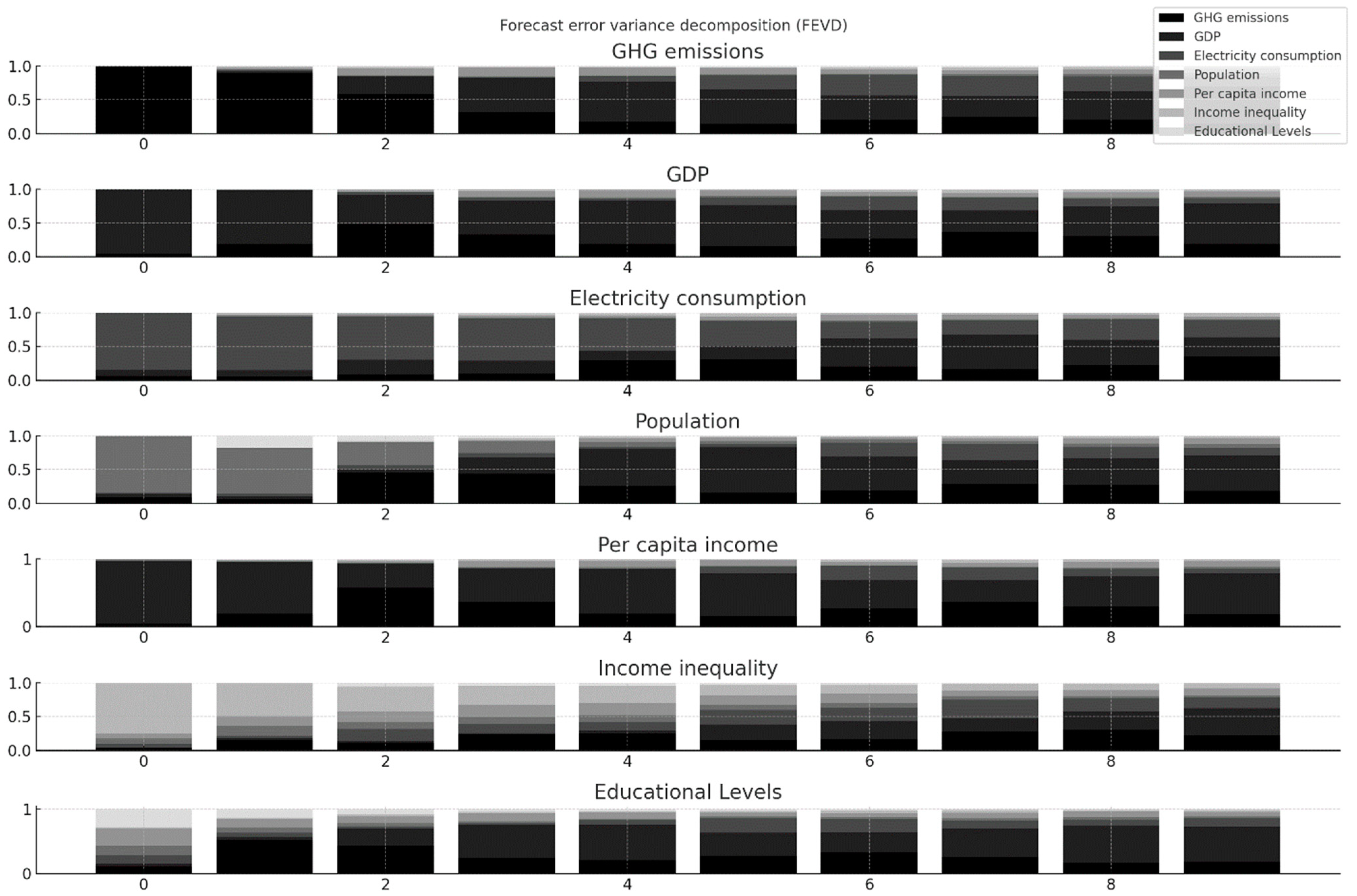
3.4.2. Forecast Error Variance Decomposition (FEVD)

Figure 2 presents a Forecast Error Variance Decomposition (FEVD) analysis, which breaks down the forecast error variance of each variable into contributions from various shocks over time. In this case, the FEVD is used to understand the relative importance of different factors in explaining the variations in GHG emissions, GDP, electricity consumption, population, per capita income, income inequality, and educational levels over different time horizons. For GHG emissions, the decomposition shows how the uncertainty or “forecast error variance” in predicting future emissions evolves as more time passes after an initial shock. Initially, at time t = 0 t = 0 t = 0, the forecast error variance of GHG emissions is entirely attributed to GHG emissions itself, as no other variables have had time to exert influence. This is a standard result, reflecting that at the initial period, the variable’s own past explains its future variance completely. As we move to later time periods (e.g., t = 2, 4, 6, 8 t = 2, 4, 6, 8 t = 2, 4, 6, 8), other variables begin to play a more significant role in explaining the variance in GHG emissions. The contribution of GHG emissions itself to its forecast error variance diminishes over time, indicating that the influence of other factors becomes more prominent. Among these factors, GDP emerges as a critical variable, increasingly explaining a larger portion of the forecast error variance in GHG emissions. This suggests that economic activities, as reflected in GDP, are significant drivers of changes in GHG emissions over time. Energy consumption also plays a notable role in contributing to the variance in GHG emissions. The relationship makes intuitive sense because higher energy consumption, especially when reliant on fossil fuels, tends to drive up emissions. The decomposition indicates that as time progresses, the impact of energy consumption on emissions becomes more pronounced, aligning with expectations of energy use being a direct determinant of emissions levels. Population and per capita income also contribute to the forecast error variance in GHG emissions. This highlights the role of demographic and economic factors in influencing emissions. An increasing population generally leads to higher aggregate demand for goods, services, and energy, thereby contributing to emissions. Similarly, rising per capita income might initially lead to higher emissions due to increased consumption, although this relationship could evolve over time depending on changes in consumption patterns and energy efficiency. Income inequality and educational levels, while showing smaller contributions compared to GDP and energy consumption, still have a noticeable impact on the forecast error variance of GHG emissions. The influence of income inequality suggests that disparities in wealth distribution may affect consumption patterns and energy use, thereby influencing emissions. The impact of educational levels may reflect how education can lead to more awareness and potentially lower emissions through changes in behavior, energy use, and support for environmental policies. The utility of the results shown in this image is significant for both researchers and policymakers. By identifying which variables contribute most to the forecast error variance of GHG emissions over time, the FEVD analysis helps to prioritize areas for intervention. For instance, if GDP and energy consumption are identified as the primary drivers of emissions variability, policies aimed at decoupling economic growth from emissions and promoting cleaner energy sources would be crucial. Understanding the contribution of population, income levels, and social factors like inequality and education further refines policy design, ensuring that interventions are comprehensive and target multiple dimensions of the problem. The FEVD analysis depicted in the image offers a detailed understanding of the dynamic relationships between GHG emissions and various economic and social variables. It reveals how different factors contribute to the variability in emissions over time, providing valuable insights for developing strategies to mitigate emissions and manage their economic and social impacts effectively.

3.4.3. Residual Correlation

A simple correlation can be observed in Table 4; however, a correlation analysis of residuals was also conducted to highlight how much of the relationships between the variables are explained by the model and how much is left in the residuals (see

Table 9. Residual correlation matrix.

	GHG Emissions	GDP	Energy Consumption	Population	Per Capita Income	Income Inequality	Educational Level
GHG emissions	1	0.64713	0.5531	0.5998	0.6962	0.0572	0.5935
GDP	0.6471	1	0.4737	0.5928	0.7479	−0.0435	0.6300
Energy consumption	0.5531	0.473719	1	0.4802	0.4572	0.0961	0.6214
Population	0.5998	0.592852	0.4802	1	0.7227	0.2146	0.5849
Per capita income	0.6962	0.747989	0.4572	0.7227	1	−0.0712	0.6334
Income inequality	0.0572	−0.043579	0.0961	0.2146	−0.0712	1	0.1293
Educational level	0.5935	0.630072	0.6214	0.5849	0.6334	0.1293	1

). The residual correlation matrix was obtained after estimating the Vector Autoregression (VAR) model with the selected variables. Once the VAR model is run, it generates residuals, which are the differences between the observed values and the values predicted by the model. These residuals are calculated for each equation in the VAR system. After obtaining the residuals, the correlation matrix was created by calculating the correlations between the residuals of each pair of variables in the model. This matrix helps to understand the unexplained correlation between variables after the relationships modeled by the VAR, indicating whether the model fully captures the dynamics among the variables.

When comparing the results of both correlation analyses, it can noted that in the simple correlation, there is a strong positive correlation with GDP, energy consumption, population, per capita income, and educational level, whereas in the residual correlation, there are moderate correlations with GDP, energy consumption, population, per capita income, and educational level. In the case of income inequality, the simple correlation showed a strong negative correlation with GHG emissions, GDP, per capita income, population, and educational level, and the residual correlation showed very weak or negligible correlations with most variables.

Conducting and analyzing a residual is crucial because it allows us to isolate the unique impact of each variable on GHG emissions, controlling for the influence of the others. This is important because the simple correlations might be driven by confounding effects where, for example, GDP and energy consumption are both correlated with GHG emissions due to their interdependence. Residual correlation analysis helps to identify the true, independent relationship between GHG emissions and each variable, providing a clearer understanding of which factors are most directly influencing emissions. This refined insight is essential for designing effective policies that target the most influential drivers of GHG emissions.

4. Discussion

4.1. Interpretation of Main Findings

After analyzing the results obtained in the calculations and modeling, different implications can be discussed. First, the strong positive correlation between GDP, per capita income, and GHG emissions highlights the relationship between economic growth and environmental impact. This suggests that larger and richer economies tend to emit more greenhouse gases, aligning with the existing literature on the Environmental Kuznets Curve (EKC), which posits that environmental impact increases in the early stages of economic development before eventually decreasing as economies become more sustainable [32]. Mexico, as a developing country, shows an expected behavior regarding the correlation between GHG and GDP since the country continues to develop and its industrial sector expands. This growth often leads to increased energy consumption, primarily from fossil fuels, which significantly contribute to GHG emissions. As noted by Osei-Kusi et al. [33], industrial activities such as manufacturing, construction, and mining are energy-intensive and typically rely on non-renewable energy sources. In particular, Mexico’s energy consumption is heavily dependent on fossil fuels, particularly oil and natural gas; despite efforts to integrate renewable energy sources, fossil fuels still dominate the energy mix [34]. Our results might indicate that the high reliance on these fuels for energy generation, transportation, and industrial processes leads to substantial CO₂ emissions. This correlation can also be explained by the rapid urbanization in Mexico, which has led to increased demand for housing, infrastructure, and transportation. This has been analyzed in other regions; for instance, in China, it was found that urban areas require significant energy for construction, heating, cooling, and mobility, all of which contribute to higher GHG emissions [35]; additionally, the expansion of cities often leads to deforestation and loss of green spaces, further exacerbating carbon emissions [18]. In an international context, our results also align with similar findings. Onofrei et al. [36] conducted a comprehensive study examining the relationship between GDP and CO₂ emissions across European Union countries, finding a positive correlation between real GDP and CO₂ emissions, indicating that higher income levels lead to increased emissions. However, the study also highlighted the increased demand for environmental protection in wealthier nations and emphasized the need for policies capable of reducing emissions during periods of economic growth. Also, in China, Caporale et al. [37] revealed that GDP growth significantly influences CO₂ emissions; such findings indicated that while economic expansion drives up emissions, the adoption of renewable energy and technological innovation can mitigate this effect. Regarding population, whereas the correlation analysis showed a positive value, the regression analysis resulted in a negative correlation, implying that as the population increases, GHG emissions decrease. Although this result highlights the need for a separate analysis to understand the behavior of demographic variables in GHG emissions, we can discuss the possible implications of such findings. As the population grows, there is a shift toward more efficient technologies and infrastructure, which can lead to reduced per capita emissions. For example, densely populated areas might invest in public transportation systems, reducing the reliance on individual vehicles and thereby lowering overall emissions. For instance, research has shown that increased energy efficiency and the transition to low-carbon technologies have contributed to reducing GHG emissions, even as economic activities and populations continue to grow. A review by Gbadeyan et al. [38] emphasizes that while economic growth is traditionally linked to higher emissions, the adoption of innovative, low-carbon energy systems has allowed some regions to decouple economic and population growth from their carbon footprints. This decoupling is critical in mitigating the environmental impact of growing populations. Moreover, another study focused on energy efficiency improvements demonstrates that structural changes in the economy, such as a shift toward less energy-intensive industries and the increased use of renewable energy sources, have played a significant role in reducing emissions despite population growth. This research underscores that energy efficiency gains and technological innovations are vital in achieving lower emissions per capita as populations increase [39]. Furthermore, economies of scale in energy production and consumption could lead to more efficient use of resources as populations grow. Larger populations may also drive innovation in energy efficiency, as there is a greater demand for sustainable practices and technologies, leading to the adoption of cleaner energy sources and better waste management practices. Huang et al. [40] argue that policies that promote sustainable urban planning and development could play a crucial role since governments may implement stricter environmental regulations, encourage renewable energy use, or incentivize businesses to adopt greener practices. According to Zeng, Ye, and Lin [41], such policies can lead to a decoupling of population growth from emissions, meaning that even as the population increases, emissions do not follow the same upward trend. Therefore, the negative relationship between population and GHG emissions may be driven by increased efficiency in resource use, technological advancements, and proactive policy measures that promote sustainable development. Together, these factors help mitigate the environmental impact of a growing population.

On the other hand, our results showed a significant negative correlation between income inequality and GHG emissions. This finding suggests that policies aimed at reducing income inequality could also have positive environmental impacts. Integrated approaches that address socio-economic disparities while promoting sustainable practices could yield dual benefits. Policymakers can develop targeted interventions in economically disadvantaged areas to improve access to clean energy, enhance energy efficiency, and promote sustainable agricultural practices. This could help in lowering GHG emissions while addressing inequality. Several studies have reported similar findings, emphasizing the complex interplay between socio-economic factors and environmental outcomes. For instance, the EKC hypothesis posits that environmental degradation initially increases with economic growth but eventually decreases as income reaches higher levels and societies can afford cleaner technologies and stricter environmental regulations. Studies have shown that income inequality can affect the shape and turning point of the EKC [42,43]. In the case of Mexico, reducing inequality may have accelerated the shift toward lower emissions at a lower income threshold. Also, research on other developing nations has also found a negative correlation between income inequality and GHG emissions. For example, a study on BRIC countries indicated that higher income inequality tends to exacerbate environmental degradation, while more equitable income distribution leads to better environmental outcomes [44]. Therefore, the significant negative correlation between income inequality and GHG emissions in Mexico underscores the importance of addressing socio-economic disparities as part of comprehensive climate strategies. This finding not only highlights the interconnectedness of social and environmental policies but also aligns with broader global research that advocates for integrated approaches to sustainable development. By leveraging these insights, Mexico can enhance its climate action plans while simultaneously promoting social equity, setting a precedent for other developing nations to follow.

The regression analysis showed that energy consumption, income inequality, and educational levels do not show statistically significant effects in our model. Their roles may be more complex, and more nuanced models might be needed to understand their impacts fully. However, results do show that GDP and per capita income are significant predictors of GHG emissions. GDP has a positive effect, indicating economic growth leads to higher emissions. Per capita income has a negative effect, suggesting that wealthier societies might adopt more efficient technologies, leading to reduced emissions. This negative relationship could imply that as income levels rise, there is a greater capacity and incentive to invest in cleaner, more sustainable technologies and practices. However, the exact mechanisms driving this relationship may involve a complex interplay of factors, such as shifts in consumer behavior, policy influences, and technological innovation. To provide a more concrete explanation, further analysis is required to explore how these factors interact and contribute to the observed reduction in emissions. Similar results have been reported in other developing economies; for example, in Africa, a study also found that economic variables like industrialization and income are significant predictors of GHG emissions [45], which is the same case as that in China, and investment and GDP proved to predict GHG emissions [46]. Therefore, these results are consistent with the Environmental Kuznets Curve (EKC) hypothesis, which posits that environmental degradation increases as an economy grows, but only up to a certain point. After this inflection point, as income reaches higher levels, environmental degradation starts to decline due to the adoption of cleaner technologies and the implementation of stricter regulations. This relationship is typically modeled using at least a second-degree polynomial function, capturing the non-linear dynamics and the inflection point characteristic of the EKC. The significance of GDP and per capita income as predictors of GHG emissions in Mexico underscores the importance of integrating economic growth strategies with environmental sustainability. This understanding can help in designing policies that promote sustainable development, balancing economic growth with the need to reduce emissions. The findings align with global research and the EKC hypothesis, suggesting that while economic growth initially leads to higher emissions, targeted investments in technology and policy interventions can eventually lead to a decrease in emissions as income levels rise. This comprehensive approach is crucial for Mexico to meet its climate goals while continuing its economic development.

As part of the regression analysis, the IRFs showed that a shock to GDP initially has a mixed response on GHG emissions, which becomes more positive over time, indicating that economic growth might lead to increased emissions. In addition, a positive response suggests that increased energy consumption and population results in higher GHG emissions, which aligns with the expectation that more energy use contributes to more emissions. This variable behavior has already been discussed and explained. However, an important highlight is that regarding educational levels and GHG emissions, the response is mostly negative, indicating that higher educational levels may contribute to lower GHG emissions, potentially through better awareness and adoption of environmentally friendly practices. This is important to discuss since education often leads to greater awareness of environmental issues and climate change, prompting individuals to adopt more sustainable practices. For instance, a study conducted at San José State University found that graduates from an intensive climate change course exhibited significant reductions in their carbon emissions due to pro-environmental behaviors adopted as a result of their education [47]. This indicates that higher education, particularly when it includes climate education, can foster long-term sustainable behavior. Also, higher educational attainment equips individuals with critical thinking skills and knowledge, enabling them to make more informed decisions about their consumption patterns, energy use, and other activities that impact GHG emissions. For example, in Benin, the impact of education on agricultural practices showed that higher education levels are associated with lower GHG emissions from agricultural activities since educated farmers are more likely to adopt sustainable farming practices that reduce emissions [48]. With this evidence, our results in this variable are consistent with other studies and contribute to arguments to support that education, particularly when it incorporates environmental and sustainability components, is a powerful tool in the fight against climate change. By raising awareness, changing behaviors, and promoting the adoption of green technologies, education contributes significantly to reducing GHG emissions. To leverage education and policies aimed at reducing inequality to lower GHG emissions, several specific strategies can be developed. Different strategies focused on environmental education can be developed, including (1) Integrating Environmental Education into Curricula: Schools and universities can include environmental science and sustainability topics as core subjects. This would increase awareness from a young age and instill environmentally friendly habits that last a lifetime. Programs could emphasize the importance of energy conservation, waste reduction, and the adoption of clean energy technologies. (2) Promoting STEM Education Focused on Sustainability: Encouraging students to pursue science, technology, engineering, and mathematics (STEM) with a focus on sustainability can drive innovation in green technologies. Scholarships and incentives for research in renewable energy, sustainable agriculture, and efficient resource use can accelerate technological advancements that reduce emissions. (3) Supporting Adult Education and Vocational Training: Offering adult education programs that teach sustainable practices, such as energy-efficient farming or green building techniques, can help reduce emissions in key sectors. Vocational training focused on renewable energy installation, maintenance, and other green jobs can also contribute to a low-carbon economy. (4) Implementing Inclusive Economic Policies: Policies that reduce economic inequality by improving access to education, healthcare, and jobs can indirectly lower emissions. For example, ensuring that disadvantaged communities have access to energy-efficient housing and affordable clean energy can reduce their carbon footprint. (5) Community-Based Education Initiatives: Establishing local workshops, seminars, and outreach programs to educate communities about the environmental impacts of their daily activities can empower individuals to make sustainable choices. These initiatives can be particularly effective in rural or underserved areas where formal education opportunities may be limited. (6) Encouraging Sustainable Consumer Behavior: Education campaigns that target consumer habits, such as reducing meat consumption, minimizing waste, or choosing sustainable products, can help lower emissions. Public awareness campaigns can highlight the environmental impact of consumer choices and promote more sustainable lifestyles. (7) Supporting Policy Advocacy and Civic Engagement: Educated populations are more likely to support and advocate for environmental policies. Providing platforms for civic engagement, such as forums or participatory planning processes, can help ensure that policies reflect the public’s desire for sustainable development and climate action.

4.2. Results Comparison

Although each result has been analyzed to understand its implications, the fact that different analyses resulted in some contradictions cannot be ignored and needs to be discussed. As observed in

Table 10. Comparison between correlation and regression results.

Variable	Pearson Correlation	Correlation Interpretation	Regression Coefficient	p-Value	Regression Interpretation
Energy Consumption	0.9827	Strong positive	0.1136	0.192	Not significant
GDP	0.9869	Strong positive	0.8018	0.001	Positive and significant
Population	0.9815	Strong positive	−3.23 × 10−6	0.061	Negative, borderline significant
Per Capita Income	0.9884	Strong positive	−0.0927	0.002	Negative and significant
Income Inequality	−0.8309	Strong negative	−76.1513	0.422	Negative, not significant
Educational Levels	0.9806	Strong positive	5.2192	0.14	Positive, not significant

, when comparing the correlation and regression results, the interpretations slightly differ. While the correlation analysis shows strong correlations for all variables, the majority of the regression values were not statistically significant.

Nevertheless, the contradictions observed between the Pearson correlation and regression analysis results in this study are not unique; they have been documented in various fields of research, particularly in studies involving complex systems with interrelated variables. For example, in a study on the relationship between energy consumption and carbon dioxide (CO₂) emissions across different countries, it was found that while energy consumption was highly correlated with CO₂ emissions in a bivariate analysis, its significance diminished when other economic factors, such as GDP and industrial output, were included in the regression model [49]. The observed contradiction arises from the fact that GDP and industrial output are closely related to energy consumption. When these factors are controlled for in a regression analysis, the unique contribution of energy consumption to CO₂ emissions may be reduced, leading to non-significant results despite strong correlations in simple bivariate analyses. Likewise, Grossman and Krueger [50] explored the Environmental Kuznets Curve (EKC) hypothesis, which posits that environmental degradation increases with economic growth up to a point, after which it decreases. Their analysis showed strong correlations between economic growth and environmental degradation (e.g., pollution), but when controlling for other factors, the expected quadratic relationship (which is central to the EKC hypothesis) was not always statistically significant. It must be noted that the EKC hypothesis involves complex interactions between economic growth, technological development, and environmental policies. The contradiction between the correlation and regression results may be due to the fact that different stages of economic development are associated with different types of economic activities and environmental impacts, which are not fully captured in a simple bivariate correlation. Also, in the study by Wilkinson and Pickett [51] on income inequality and health outcomes, a strong negative correlation was found between income inequality and population health measures in many countries. However, when factors such as public healthcare spending and education levels were included in the regression models, the direct impact of income inequality on health outcomes often became statistically insignificant. This contradiction can be attributed to the fact that income inequality interacts with multiple social determinants of health, such as access to education, healthcare, and social services. In regression models that account for these interacting factors, the unique contribution of income inequality may be obscured, leading to non-significant coefficients even in the presence of strong correlations. Finally, Martínez-Zarzoso and Maruotti [52] examined the relationship between urbanization and carbon emissions in developing countries. They found a strong positive correlation between urbanization and carbon emissions. However, in regression models that included variables such as economic structure, energy mix, and technological development, the effect of urbanization on carbon emissions was often not statistically significant. Urbanization is closely linked to various factors, such as industrialization, changes in energy consumption patterns, and infrastructure development. When these factors are controlled for in a regression model, the direct effect of urbanization on carbon emissions may be diminished, resulting in non-significant regression coefficients despite strong bivariate correlations.

As a consequence of the foregoing, recognizing that a strong correlation does not necessarily translate to a significant independent effect in a multivariate context allows policymakers to design more targeted interventions. For example, policies aiming to reduce GHG emissions might focus on improving energy efficiency and promoting clean technologies rather than solely targeting energy consumption. The findings underscore the need for a holistic approach that considers the interactions between multiple factors. For instance, while economic growth (GDP) shows a clear link to GHG emissions, it is essential to also consider the roles of income distribution, technological adoption, and educational initiatives in crafting comprehensive environmental policies. Policymakers should be aware of the potential for multicollinearity and overlapping effects when designing policies. This awareness encourages flexibility in policy design, allowing for adjustments as more data become available and as the interdependencies between variables are better understood. The contradictions highlight the importance of using both bivariate and multivariate analyses to inform decision-making. While correlations provide valuable initial insights, regression analyses offer a more nuanced understanding of the relationships between variables, which is crucial for effective policy implementation.

4.3. Hypothesis Verification

• Hypothesis 1 (H1): GDP is positively correlated with GHG emissions in Mexico.
  Proven: This study found a very high positive correlation between GDP and GHG emissions, confirming that economic growth in Mexico is strongly associated with increased emissions. This result aligns with the Environmental Kuznets Curve (EKC) hypothesis, which posits that economic growth initially leads to higher environmental degradation before potentially declining as the economy matures and adopts cleaner technologies. The findings are consistent with global patterns and similar studies in other countries like China and the European Union, where economic growth has been shown to significantly influence GHG emissions.
• Hypothesis 2 (H2): Energy consumption has a positive and significant impact on GHG emissions in Mexico.
  Partially proven: While the correlation analysis showed a strong positive relationship between energy consumption and GHG emissions, the regression analysis indicated that this relationship was not statistically significant. This suggests that while energy consumption is correlated with higher emissions, other factors may also play a significant role, complicating the direct impact of energy consumption alone. This finding suggests a more complex interaction, possibly involving the types of energy sources used and the efficiency of energy consumption, and it aligns with findings in other studies where energy consumption’s impact varies depending on the broader economic context.
• Hypothesis 3 (H3): Population growth is positively correlated with GHG emissions in Mexico.
  Proven with a twist: The correlation analysis found a positive relationship between population growth and GHG emissions. However, the regression analysis revealed a negative, though borderline significant, relationship. This unexpected result could indicate that as the population grows, technological and infrastructural efficiencies might offset the expected increase in emissions, leading to a reduction in per capita emissions. This result suggests a need for further analysis but aligns with theories suggesting that population growth can sometimes drive the adoption of more efficient technologies and infrastructure.
• Hypothesis 4 (H4): Per capita income is positively correlated with GHG emissions in Mexico.
  Disproven: Contrary to the hypothesis, this study found a negative and significant relationship between per capita income and GHG emissions. This suggests that as income increases, there may be greater adoption of energy-efficient technologies or sustainable practices that reduce overall emissions. This finding is consistent with parts of the EKC hypothesis, where wealthier societies eventually reduce their environmental impact as they can afford to invest in cleaner technologies.
• Hypothesis 5 (H5): Income inequality (measured by the Gini coefficient) is negatively correlated with GHG emissions in Mexico.
  Proven: This study confirmed a significant negative correlation between income inequality and GHG emissions. This suggests that higher income inequality might be associated with lower emissions, possibly because of reduced consumption among lower-income groups who lack access to energy-intensive goods and services. This finding aligns with some studies that indicate income inequality can influence consumption patterns and environmental outcomes, though the exact mechanisms may be complex and multifaceted.
• Hypothesis 6 (H6): Educational levels are negatively correlated with GHG emissions in Mexico.
  Disproven: The correlation analysis showed a positive relationship between educational levels and GHG emissions, which contradicts the hypothesis. This may indicate that higher education levels, while contributing to economic growth (and thus emissions), also reflect a society where higher levels of consumption and economic activity drive emissions upward. However, the Granger causality analysis suggested that higher education might still play a role in reducing emissions indirectly through better environmental practices, even if this effect was not immediately apparent in the direct correlation.

This study’s results generally align with existing theories like the EKC hypothesis and findings from other countries, particularly in the positive relationship between economic growth (GDP) and GHG emissions. The complex and sometimes contradictory findings regarding population, income inequality, and education reflect the nuanced and multifaceted nature of socio-economic factors on environmental outcomes. These results highlight the importance of considering a broad range of factors and the interactions between them when analyzing GHG emissions. Overall, the hypotheses were largely proven or partially proven, with some unexpected findings that add depth to the discussion. This study contributes to the understanding of how socio-economic factors influence GHG emissions in Mexico and offers valuable insights for policy-making aimed at reducing emissions while promoting sustainable development.

4.4. Policy Implications

Table 11. Policy suggestions derived from main findings.

Driver of GHG Emissions	Policy Implications	Policy Recommendations
Gross Domestic Product (GDP)	Economic growth is strongly associated with increased GHG emissions. There is a need to decouple economic growth from environmental degradation.	- Promote green growth through incentives for clean technologies. - Implement sustainable industrialization with sector-specific emission reduction targets. - Support SMEs in adopting green technologies.
Energy Consumption	High energy consumption correlates with higher GHG emissions. Transitioning to cleaner energy sources is critical.	- Expand investment in renewable energy infrastructure. - Implement nationwide energy efficiency programs. - Modernize the energy grid to better integrate renewable energy.
Population Growth	Population growth increases resource demand, leading to higher emissions. Efficiency gains and sustainable urbanization can mitigate this impact.	- Promote sustainable urban planning with compact, resource-efficient cities. - Support population control indirectly through education and healthcare. - Strengthen rural development programs to reduce urban migration.
Per Capita Income	Higher per capita income may lead to reduced GHG emissions through the adoption of energy-efficient technologies.	- Encourage sustainable consumption through eco-labeling and awareness campaigns. - Provide subsidies for green products and technologies. - Implement progressive environmental taxation to discourage high-consumption activities.
Income Inequality (Gini Coefficient)	Reducing income inequality could lower GHG emissions by promoting equitable access to clean technologies.	- Ensure equitable access to clean technologies for low-income households. - Develop inclusive economic policies that promote green jobs and fair wages. - Use environmental tax revenues to fund social programs aimed at reducing inequality.
Educational Levels	Higher education levels can drive economic activity and consumption but also promote sustainable practices.	- Integrate environmental education into curriculums at all levels. - Develop vocational training programs focused on green skills. - Launch public awareness campaigns on the importance of reducing GHG emissions.

provides a summary of how various socio-economic factors influence greenhouse gas (GHG) emissions in Mexico and outlines potential public policy recommendations to address these influences. The policy implications derived from this research’s findings underscore the need for a multi-faceted approach to reducing GHG emissions in Mexico. By targeting the key drivers of emissions identified in our study—economic growth, energy consumption, population dynamics, income distribution, and education—Mexico can design effective policies that not only mitigate climate change but also promote sustainable development. These policies must be integrated, adaptive, and inclusive, ensuring that they address the complex socio-economic factors that influence GHG emissions while supporting the country’s broader economic and social goals.

However, such policy implications and possible strategies emerge not only from the results we obtained but also from existing studies that have reported successful cases that support the approaches suggested. For example, several European countries have reported important successful initiatives. Germany’s Energiewende illustrates the effective decoupling of economic growth from GHG emissions through significant investment in renewable energy. By prioritizing wind and solar power, Germany reduced emissions while boosting job creation and innovation, demonstrating the potential of a strong commitment to clean energy [53]. Also, in Germany, the dual education system promotes green skills through vocational training in renewable energy and energy efficiency, contributing to the country’s leadership in green technologies and emissions reductions [54]. Other examples include Sweden’s industrial emissions reduction, which highlights the success of combining carbon taxes with subsidies for low-carbon technologies [55], and Denmark’s smart grid development, which demonstrates how advanced grid technology can efficiently integrate renewable energy, reducing energy waste and enhancing reliability [56]. Also, Norway’s electric vehicle subsidies have made EVs widely accessible, resulting in significant reductions in transportation emissions [57]. This case underscores the effectiveness of financial incentives in shifting consumer behavior toward sustainable options. Also in Europe, Finland’s environmental education programs have effectively raised environmental awareness and fostered sustainable practices, contributing to long-term reductions in national GHG emissions [58], while the UK’s “Act on CO₂” campaign shows how public awareness initiatives can successfully reduce energy use and emissions by educating the public on the environmental impact of their daily activities [59]. In North America, for example, British Columbia’s carbon tax demonstrates the efficacy of progressive environmental taxation in reducing fuel consumption and emissions. The tax’s revenue-neutral design, which funds green initiatives and rebates for low-income households, highlights the balance between environmental and social goals [60]. In addition, California’s energy efficiency programs show how comprehensive measures like strict building codes and appliance standards can reduce energy consumption per capita while supporting economic growth [61]. Also, in Latin America, some cases are worth mentioning, such as Costa Rica’s renewable energy success, with over 98% of its electricity from renewable sources, exemplifying the impact of focused policy efforts. Strong governmental commitment and infrastructure investment have allowed Costa Rica to significantly reduce its carbon footprint [62]. On the other hand, Brazil’s rural development programs have successfully reduced deforestation and rural poverty by improving infrastructure and promoting sustainable agriculture, illustrating the role of rural development in mitigating GHG emissions [63].

These case studies highlight the potential of well-targeted public policies to significantly reduce GHG emissions while promoting economic growth, social equity, and sustainability. Each offers valuable insights that Mexico and similar developing countries can adapt to its specific context.

5. Conclusions

The analysis of greenhouse gas (GHG) emissions in Mexico reveals several key socio-economic drivers with varying degrees of influence. GDP, energy consumption, and population are positively correlated with GHG emissions, confirming their significant environmental impact. Economic growth, increased energy use, and a growing population contribute to higher emissions, aligning with global patterns observed in the literature. The positive correlation between per capita income and GHG emissions highlights the environmental costs associated with higher income and increased consumption. This suggests that as incomes rise, so does the demand for goods and services that generate emissions. The negative correlation between income inequality and GHG emissions indicates a complex dynamic. Higher inequality might reduce overall consumption but also limit access to cleaner technologies, suggesting that policies addressing inequality could have nuanced effects on emissions. Although higher educational levels are directly correlated with increased GHG emissions, the broader economic benefits of education suggest its crucial role in long-term sustainable development. Educated populations are more likely to adopt and advocate for sustainable practices and technologies.

The Granger causality analysis underscores that GDP and per capita income are strong predictors of GHG emissions in Mexico. Energy consumption and population also show significant causative effects at certain lags. In contrast, income inequality and educational levels do not exhibit direct causative impacts on emissions. This highlights the importance of focusing on economic activities to manage emissions effectively. The Vector Autoregression (VAR) analysis confirms that GDP and past GHG emissions are significant drivers of current emissions. While other variables are important, their direct causal impacts on GHG emissions are less evident in this model. Based on these findings, several recommendations can be made. First, promoting renewable energy and implementing policies that decouple economic growth from GHG emissions are crucial steps. Encouraging behaviors and consumption patterns that are environmentally sustainable, possibly through tax incentives or subsidies for green products, can also help manage emissions. Developing policies that reduce inequality and promote equitable access to clean technologies is important to mitigate indirect effects on emissions.

Strengthening climate and environmental education at all levels can foster long-term sustainable behaviors and support for green policies. Utilizing universities and schools as hubs for sustainability practices and innovations can leverage educational institutions’ influence on emissions. Developing integrated policies that address multiple factors simultaneously, recognizing the interconnectedness of economic growth, energy consumption, population dynamics, and education, is essential. Using advanced econometric models to continuously analyze and understand the causative relationships between socio-economic factors and GHG emissions will allow for more targeted and effective interventions. By addressing these key areas, policymakers can design strategies that effectively manage and reduce GHG emissions, aligning with sustainable development goals and mitigating the adverse effects of climate change.

Nevertheless, while our analysis provides important insights into the socio-economic drivers of GHG emissions in Mexico and offers valuable policy recommendations, it is essential to approach these findings with caution. The selected variables and units, such as the use of aggregate GDP, total energy consumption, and general measures of income inequality and education, may not capture all the nuances and sector-specific dynamics that influence emissions. We encourage the development of further research with alternative measures, such as disaggregating GDP into its industrial and service components or considering more production-related inequality indicators, which could provide deeper and potentially more accurate insights. Additionally, the focus on total energy consumption without distinguishing between renewable and non-renewable sources or energy efficiency measures may limit the scope of our conclusions. These limitations suggest that while our findings are significant, they should be interpreted within the context of these constraints. Future research incorporating more refined and sector-specific variables could further enhance our understanding of the complex relationships between socio-economic factors and GHG emissions.

References

1. Tuckett, R. Greenhouse Gases. In Encyclopedia of Analytical Science; Worsfold, P., Townshend, A., Poole, C., Miró, M., Eds.; Elsevier: Amsterdam, The Netherlands, 2018; pp. 362–372. [Google Scholar] [CrossRef]
2. CCCH-Center for Climate Change and Health. Climate Change 101: Climate Science Basics. Available online: https://climatehealthconnect.org/wp-content/uploads/2016/09/Climate101.pdf (accessed on 5 July 2024).
3. NRC. Verifying Greenhouse Gas Emissions: Methods to Support International Climate Agreements; National Academies Press: Washington, DC, USA, 2010. [Google Scholar]
4. NOS-National Ocean Service. Global and Regional Sea Level Rise Scenarios for the United States. Available online: https://cdn.oceanservice.noaa.gov/oceanserviceprod/hazards/sealevelrise/noaa-nos-techrpt01-global-regional-SLR-scenarios-US.pdf (accessed on 5 July 2024).
5. Gilli, M.; Calcaterra, M.; Emmerling, J.; Granella, F. Climate change impacts on the within-country income distributions. J. Environ. Econ. Manag. 2024, 127, 103012. [Google Scholar] [CrossRef]
6. Gomez-Zavaglia, A.; Mejuto, J.C.; Simal-Gandara, J. Mitigation of emerging implications of climate change on food production systems. Food Res. Int. 2020, 134, 109256. [Google Scholar] [CrossRef]
7. Li, K.; Pan, J.; Xiong, W.; Xie, W.; Ali, T. The impact of 1.5 °C and 2.0 °C global warming on global maize production and trade. Sci. Rep. 2022, 12, 17268. [Google Scholar] [CrossRef]
8. IPCC-Intergovernmental Panel on Climate Change. Climate Change and Land. Available online: https://www.ipcc.ch/site/assets/uploads/sites/4/2021/02/210202-IPCCJ7230-SRCCL-Complete-BOOK-HRES.pdf (accessed on 4 July 2024).
9. Gupta, A.; Venkataraman, S. Insurance and climate change. Curr. Opin. Environ. Sustain. 2024, 67, 101412. [Google Scholar] [CrossRef]
10. Benesch, T.; Sergeeva, M.; Wainstock, D.; Miller, J. Climate change, health, and human rights: Calling on states to address the health risks of climate change, through the Inter-American Court of Human Rights. Lancet Reg. Health-Am. 2024, 34, 100801. [Google Scholar] [CrossRef]
11. WHO-World Health Organization. Climate Change and Health. Available online: https://apps.who.int/gb/ebwha/pdf_files/EB154/B154_25-en.pdf (accessed on 5 July 2024).
12. IDMC-Internal Displacement Monitoring Centre. Global Report on International Displacement. Available online: https://api.internal-displacement.org/sites/default/files/publications/documents/IDMC-GRID-2024-Global-Report-on-Internal-Displacement.pdf (accessed on 6 July 2024).
13. The World Bank. Gender and Forced Displacement in Cities. Available online: https://documents1.worldbank.org/curated/en/099110323161023204/pdf/P1749910706c6c014086e903e0437504040.pdf (accessed on 5 July 2024).
14. Carleton, T. Crop-damaging temperatures increase suicide rates in India. Proc. Natl. Acad. Sci. USA 2017, 114, 8746–8751. [Google Scholar] [CrossRef]
15. Mullis, J.; White, C. Temperature and mental health: Evidence from the spectrum of mental health outcomes. J. Health Econ. 2019, 68, 102240. [Google Scholar] [CrossRef]
16. Wiedenhofer, D.; Virag, D.; Kalt, G.; Plank, B.; Streeck, J.; Pichler, M.; Mayer, A.; Krausmann, F.; Brockway, P.; Schaffartzink, A. A systematic review of the evidence on decoupling of GDP, resource use and GHG emissions, part I: Bibliometric and conceptual mapping. Environ. Res. Lett. 2020, 15, 063002. [Google Scholar] [CrossRef]
17. Mugableh, M. Analysing the CO2 Emissions Function in Malaysia: Autoregressive Distributed Lag Approach. Procedia Econ. Financ. 2013, 5, 571–580. [Google Scholar] [CrossRef]
18. Liu, Y.; Gao, C.; Lu, Y. The impact of urbanization on GHG emissions in China: The role of population density. J. Clean. Prod. 2017, 157, 299–309. [Google Scholar] [CrossRef]
19. Wang, Q.; Li, L. The effects of population aging, life expectancy, unemployment rate, population density, per capita GDP, urbanization on per capita carbon emissions. Sustain. Prod. Consum. 2021, 28, 760–774. [Google Scholar] [CrossRef]
20. Vera, M.; Navarro, A.; Samperio, J. Climate change and income inequality: An I-O analysis of the structure and intensity of the GHG emissions in Mexican households. Energy Sustain. Dev. 2021, 60, 15–25. [Google Scholar] [CrossRef]
21. Martin, E.; Chan, N.; Shaheen, S. How Public Education on Ecodriving Can Reduce Both Fuel Use and Greenhouse Gas Emissions. Transp. Res. Rec. J. Transp. Res. Board 2012, 2287, 163–173. [Google Scholar] [CrossRef]
22. Zaland, Z.; Imamoglu, H. Revisiting the environmental Kuznets curve hypothesis in the context of renewable and non-renewable energy in China. Bus. Manag. Stud. Int. J. 2024, 12, 240–252. [Google Scholar] [CrossRef]
23. Mohammed, S.; Rashid, A.; Ghosal, K.; Al-Dalahmeh, M.; Alsafadi, K.; Szabó, S.; Oláh, J.; Alkerdi, A.; Ocwa, A.; Harsanyi, E. Assessment of the environmental kuznets curve within EU-27: Steps toward environmental sustainability (1990–2019). Environ. Sci. Ecotechnol. 2024, 18, 100312. [Google Scholar] [CrossRef] [PubMed]
24. Wang, Q.; Zhang, F.; Li, R. Revisiting the environmental kuznets curve hypothesis in 208 counties: The roles of trade openness, human capital, renewable energy and natural resource rent. Environ. Res. 2023, 216, 114637. [Google Scholar] [CrossRef] [PubMed]
25. Al-mulali, U.; Tang, C.; Ozturk, I. Estimating the Environment Kuznets Curve hypothesis: Evidence from Latin America and the Caribbean countries. Renew. Sustain. Energy Rev. 2015, 50, 918–924. [Google Scholar] [CrossRef]
26. Ghaderi, Z.; Saboori, B.; Khoshkam, M. Revisiting the Environmental Kuznets Curve Hypothesis in the MENA Region: The Roles of International Tourist Arrivals, Energy Consumption and Trade Openness. Sustainability 2023, 15, 2553. [Google Scholar] [CrossRef]
27. Espoir, D.; Sunge, R. Co2 emissions and economic development in Africa: Evidence from a dynamic spatial panel model. J. Environ. Manag. 2021, 300, 113617. [Google Scholar] [CrossRef]
28. Kar, A. Environmental Kuznets curve for CO2 emissions in Baltic countries: An empirical investigation. Environ. Sci. Pollut. Res. 2022, 29, 47189–47208. [Google Scholar] [CrossRef]
29. Fomby, T.; Johnson, S.; Hill, R. Advanced Econometric Methods; Springer Science+Business: New York, NY, USA, 2012. [Google Scholar]
30. Benesty, J.; Chen, J.; Huang, Y.; Cohen, I. Pearson Correlation Coefficient. In Noise Reduction in Speech Processing; Springer Topics in Signal Processing; Springer: Berlin/Heidelberg, Germany, 2009; Volume 2, pp. 1–4. [Google Scholar]
31. Montgomery, D.; Peck, E.; Vining, G. Introduction to Linear Regression Analysis; John Wiley & Sons Inc.: Hoboken, NJ, USA, 2012. [Google Scholar]
32. Guo, X.; Shabaz, M. The existence of environmental Kuznets curve: Critical look and future implications for environmental management. J. Environ. Manag. 2024, 351, 119648. [Google Scholar] [CrossRef] [PubMed]
33. Osei-Kusi, F.; Wu, C.; Tetteh, S.; Castillo, W. The dynamics of carbon emissions, energy, income, and life expectancy: Regional comparative analysis. PLoS ONE 2024, 19, e0293451. [Google Scholar] [CrossRef] [PubMed]
34. Escamilla-García, P.E.; Fernández-Rodríguez, E.; Jimenez-Castañeda, M.E.; Morales-Castro, J.A. Analysis of the progress and potential of energy generation from renewable sources in Latin America. Lat. Am. Res. Rev. 2023, 58, 383–402. [Google Scholar] [CrossRef]
35. Xiong, X.; Zhang, L.; Hao, Y.; Zhang, P.; Shi, Z.; Zhang, T. How urbanization and ecological conditions affect urban diet-linked GHG emissions: New evidence from China. Resour. Conserv. Recycl. 2022, 176, 105903. [Google Scholar] [CrossRef]
36. Onofrei, M.; Vatamanu, A.; Cigu, E. The Relationship Between Economic Growth and CO2 Emissions in EU Countries: A Cointegration Analysis. Front. Environ. Sci. 2022, 10, 934885. [Google Scholar] [CrossRef]
37. Caporale, G.; Quiroga, G.; Alana, L. Analysing the relationship between CO2 emissions and GDP in China: A fractional integration and cointegration approach. J. Innov. Entrep. 2021, 10, 32. [Google Scholar] [CrossRef]
38. Gbadeyan, O.; Muthivhi, J.; Linganiso, L.; Deenadayalu, N. Decoupling Economic Growth from Carbon Emissions: A Transition toward Low-Carbon Energy Systems—A Critical Review. Clean Technol. 2024, 6, 1076–1113. [Google Scholar] [CrossRef]
39. Landolsi, M.; Miled, K. Reducing GHG Emissions by Improving Energy Efficiency: A Decomposition Approach. Environ. Model. Assess. 2024, 29, 767–780. [Google Scholar] [CrossRef]
40. Huang, Y.; Yang, Y.; Ren, H.; Ye, L.; Liu, Q. From Urban Design to Energy Sustainability: How Urban Morphology Influences Photovoltaic System Performance. Sustainability 2024, 16, 7193. [Google Scholar] [CrossRef]
41. Zeng, L.; Ye, A.; Lin, W. Deepening decoupling for sustainable development: Evidence from threshold model. Energy Effic. 2022, 15, 33. [Google Scholar] [CrossRef]
42. Balezentis, T.; Liobikiene, G.; Streimikiene, D.; Sun, K. The impact of income inequality on consumption-based greenhouse gas emissions at the global level: A partially linear approach. J. Environ. Manag. 2020, 267, 110635. [Google Scholar] [CrossRef]
43. Sahu, S.; Patnaik, U. The tradeoffs between GHGs emissions, income inequality and productivity. Energy Clim. Chang. 2020, 1, 100014. [Google Scholar] [CrossRef]
44. He, Z.; Li, J.; Ayub, B. How do income inequality, poverty and industry 4.0 affect environmental pollution in South Asia: New insights from quantile regression. Heliyon 2024, 10, e33397. [Google Scholar] [CrossRef]
45. Apeaning, R.; Labaran, M. Club convergence of per capita greenhouse gas emissions in Africa: A multi-sectoral analysis of trends and drivers. Sustain. Futures 2024, 7, 100191. [Google Scholar] [CrossRef]
46. Ze, F.; Wong, W.; Alhasan, T.; Shraah, A.; Ali, A.; Muda, I. Economic development, natural resource utilization, GHG emissions and sustainable development: A case study of China. Resour. Policy 2023, 83, 103596. [Google Scholar] [CrossRef]
47. Cordero, E.; Centeno, D.; Todd, A. The role of climate change education on individual lifetime carbon emissions. PLoS ONE 2020, 15, e0206266. [Google Scholar] [CrossRef]
48. Jacquet, I.; Zhang, J.; Wang, K.; Liang, S.; Fu, S.; Liu, S. Mitigating greenhouse gas emissions from agriculture in Benin: Spatial estimation and reduction options. Environ. Dev. Sustain. 2023, 5, 1–15. [Google Scholar] [CrossRef]
49. Ang, J. CO2 emissions, energy consumption, and output in France. Energy Policy 2007, 35, 4772–4778. [Google Scholar] [CrossRef]
50. Grossman, G.M.; Krueger, A.B. Economic growth and the environment. Q. J. Econ. 1995, 110, 353–377. [Google Scholar] [CrossRef]
51. Wilkinson, R.; Pickett, K. Income inequality and population health: A review and explanation of the evidence. Soc. Sci. Med. 2006, 62, 1768–1784. [Google Scholar] [CrossRef]
52. Martínez-Zarzoso, I.; Maruotti, A. The impact of urbanization on CO2 emissions: Evidence from developing countries. Ecol. Econ. 2011, 70, 1344–1353. [Google Scholar] [CrossRef]
53. Sonneschein, J.; Hennicke, P. The German Energiewende A Transition towards an Efficient, Sufficient Green Energy Economy; Lund University: Lund, Sweden, 2015. [Google Scholar]
54. Auktor, G.; Green Industrial Skills for a Sustainable Future. United Nations Industrial Development Organization (UNIDO). Available online: https://www.unido.org/sites/default/files/files/2021-02/LKDForum-2020_Green-Skills-for-a-Sustainable-Future.pdf (accessed on 19 August 2024).
55. Andersson, J. Carbon Taxes and CO2 Emissions: Sweden as a Case Study. Am. Econ. J. Econ. Policy 2019, 11, 1–30. [Google Scholar] [CrossRef]
56. Lund, H.; Thellufsen, J.; Sorknæs, P.; Mathiesen, B.; Chang, M.; Madsen, P.; Kany, M.; Skov, I. Smart energy Denmark. A consistent and detailed strategy for a fully decarbonized society. Renew. Sustain. Energy Rev. 2022, 168, 112777. [Google Scholar] [CrossRef]
57. Springel, K. It’s Not Easy Being “Green”: Lessons from Norway’s Experience with Incentives for Electric Vehicle Infrastructure. Rev. Environ. Econ. Policy 2021, 15, 352–359. [Google Scholar] [CrossRef]
58. Salonen, A.; Konkka, J. An ecosocial approach to wellbeing: A solution to the wicked problems in the era of anthropocene. J. Clean. Prod. 2015, 13, 19–34. [Google Scholar] [CrossRef]
59. Clark, H. The ACT ON CO2 Campaign. Department for Transport. Available online: https://www.zemo.org.uk/assets/workingdocuments/PCWG-P-08-10%20Act%20on%20CO2%20Review.pdf (accessed on 19 August 2024).
60. Murray, B.; Rivers, N. British Columbia’s revenue-neutral carbon tax: A review of the latest “grand experiment” in environmental policy. Energy Policy 2015, 86, 674–683. [Google Scholar] [CrossRef]
61. NRDC. California’s Energy Efficiency Success Story: Saving Billions of Dollars and Curbing Tons of Pollution. Available online: https://www.nrdc.org/sites/default/files/ca-success-story-FS.pdf (accessed on 19 August 2024).
62. Gonzalez, E. Costa Rica 100% Renewable: Keys and Lessons from a Successful Electric Power Policy. Available online: https://library.fes.de/pdf-files/bueros/mexiko/13389.pdf (accessed on 19 August 2024).
63. Chiavari, J.; Antonaccio, L. Brazilian Agricultural Mitigation and Adaptation Policies: Towards Just Transition. Available online: https://www.climatepolicyinitiative.org/publication/brazilian-agricultural-mitigation-and-adaptation-policies-towards-just-transition/ (accessed on 19 August 2024).
Figure 1. Impulse response functions (IRF).
Sustainability 16 07668 g001
Figure 2. Forecast Error Variance Decomposition (FEVD).
Sustainability 16 07668 g002