

The Role of the Real Estate Sector in the Economy: Cross-National Disparities and Their Determinants


Abstract
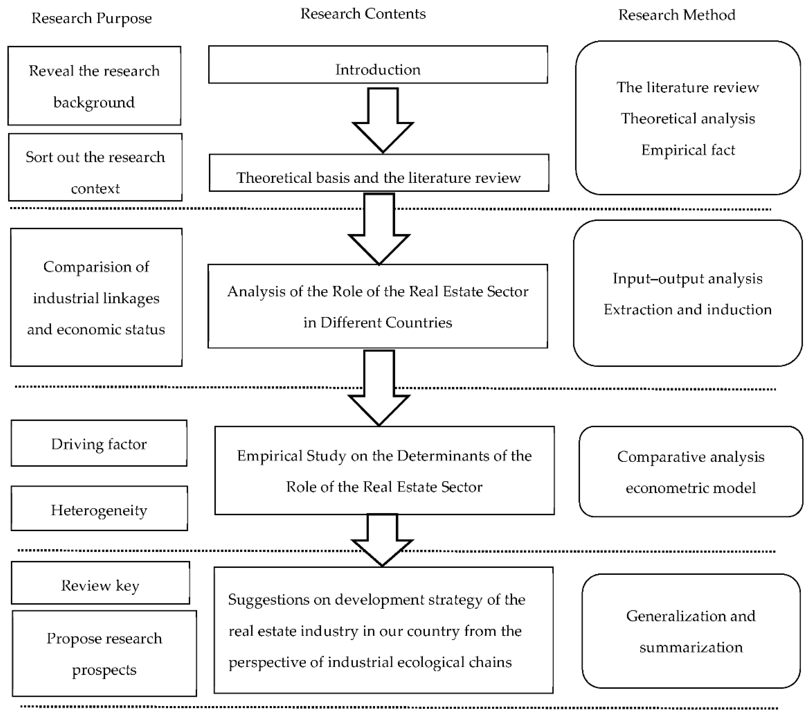
:1. Introduction
2. Analysis of the Role of the Real Estate Sector in Different Countries
2.1. Methods
2.2. Data
2.3. Results
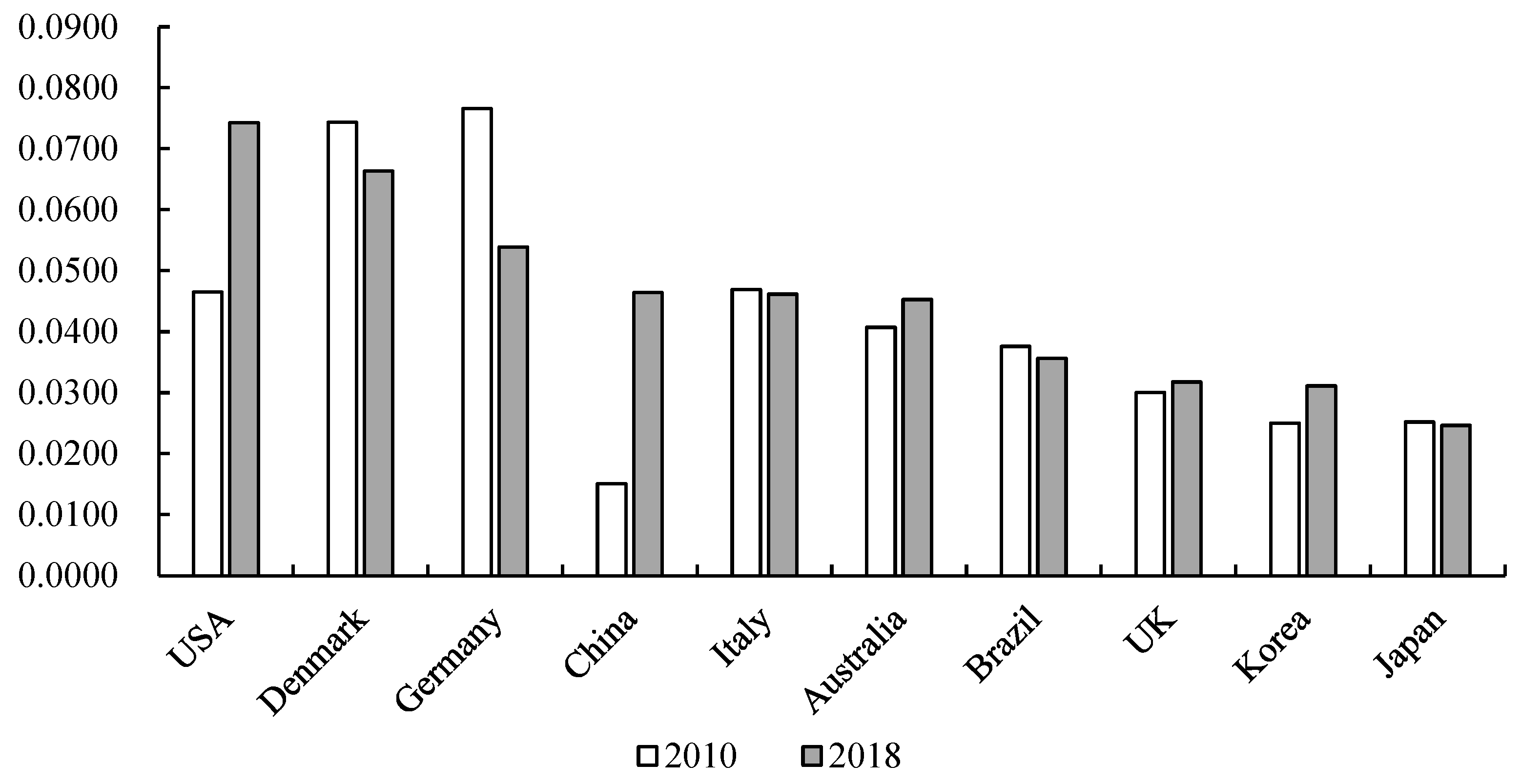
- (1)
- Comparison of inter-sectoral linkages
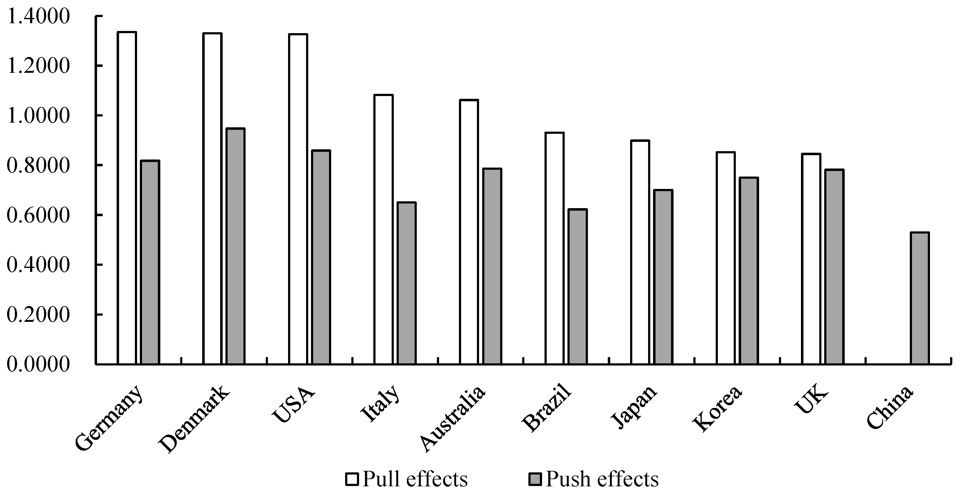
- (2)
- Comparison of pull and push effects on the economy
3. Empirical Study on the Determinants of the Role of the Real Estate Sector
3.1. Model
3.2. Descriptive Analysis
3.3. Empirical Results
- (1)
- Regression Analysis
- (2)
- Robustness tests
- (3)
- Heterogeneity tests
4. Discussion
5. Conclusions and Implications
Author Contributions
Funding
Institutional Review Board Statement
Data Availability Statement
Conflicts of Interest
Appendix A. Direct Input Indicator of the Real Estate Sector from 2010 to 2018

| No. | Country/Region | 2010 | 2014 | 2018 | |||
| Sector | Value | Sector | Value | Sector | Value | ||
| 1 | Switzerland | D41T43 | 0.0702 | D41T43 | 0.0651 | D41T43 | 0.05567 |
| D64T66 | 0.0530 | D64T66 | 0.0438 | D69T75 | 0.04021 | ||
| 2 | Türkiye | D41T43 | 0.0168 | D41T43 | 0.0306 | D41T43 | 0.04050 |
| D23 | 0.0108 | D23 | 0.0256 | D23 | 0.03283 | ||
| 3 | Japan | D64T66 | 0.0746 | D64T66 | 0.0712 | D64T66 | 0.08404 |
| D41T43 | 0.0261 | D41T43 | 0.0342 | D68 | 0.03371 | ||
| 4 | Cambodia | D35 | 0.0513 | D64T66 | 0.0395 | D64T66 | 0.03917 |
| D61 | 0.0283 | D61 | 0.0289 | D61 | 0.03028 | ||
| 5 | Thailand | D64T66 | 0.0702 | D64T66 | 0.0835 | D64T66 | 0.06453 |
| D35 | 0.0602 | D35 | 0.0579 | D35 | 0.04262 | ||
| 6 | Tunisia | D64T66 | 0.0411 | D64T66 | 0.0536 | D64T66 | 0.05853 |
| D35 | 0.0126 | D35 | 0.0090 | D35 | 0.01086 | ||
| 7 | Greece | D41T43 | 0.0437 | D64T66 | 0.0489 | D64T66 | 0.02529 |
| D64T66 | 0.0321 | D41T43 | 0.0265 | D41T43 | 0.02260 | ||
| 8 | Argentina | D41T43 | 0.0233 | D41T43 | 0.0242 | D41T43 | 0.02084 |
| D77T82 | 0.0133 | D77T82 | 0.0138 | D45T47 | 0.01355 | ||
| 9 | Lithuania | D16 | 0.0411 | D68 | 0.0849 | D68 | 0.05101 |
| D45T47 | 0.0227 | D77T82 | 0.0349 | D77T82 | 0.02893 | ||
| 10 | Slovakia | D41T43 | 0.0983 | D64T66 | 0.0654 | D68 | 0.07392 |
| D68 | 0.0580 | D68 | 0.0571 | D64T66 | 0.05415 | ||
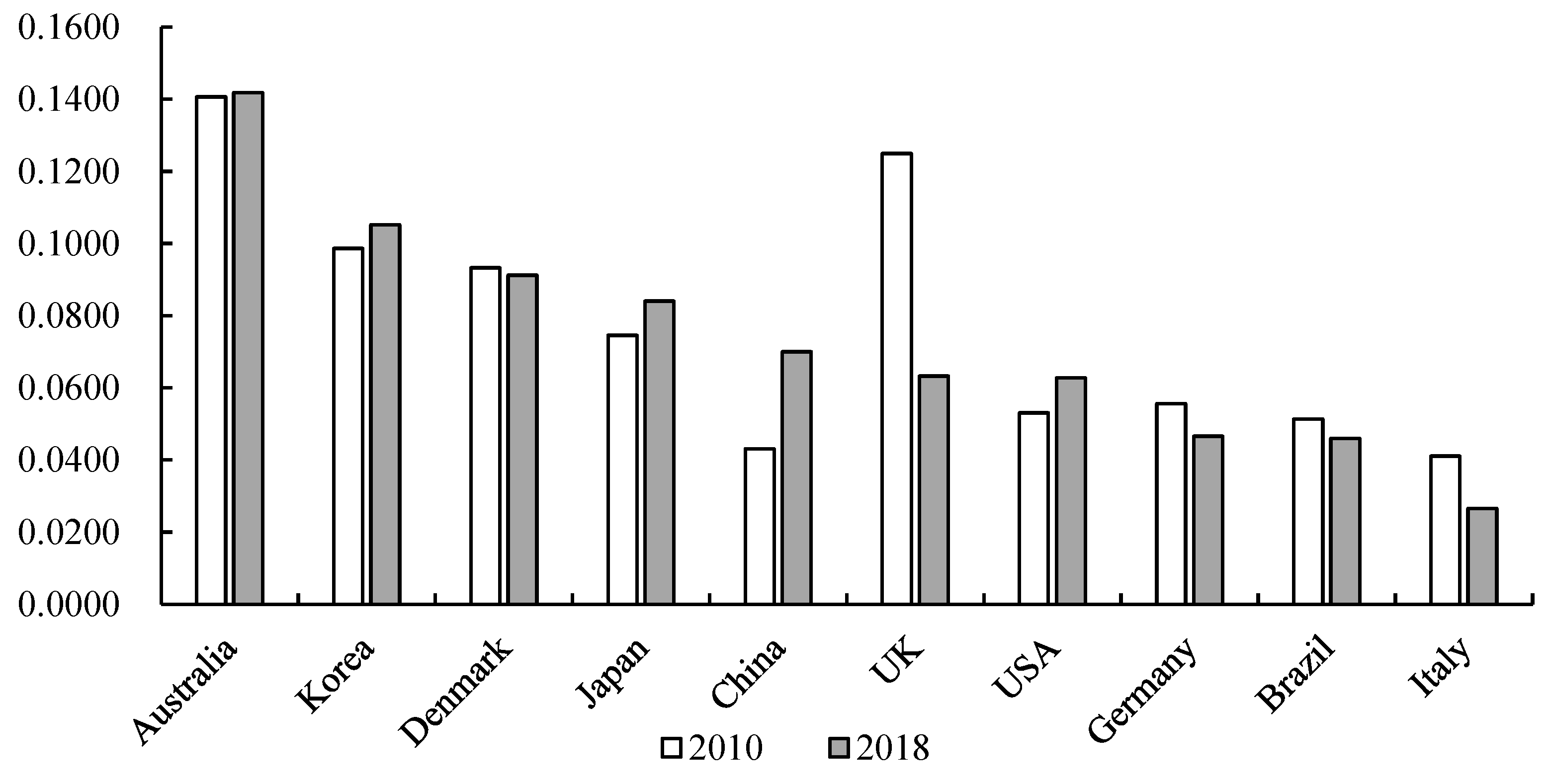
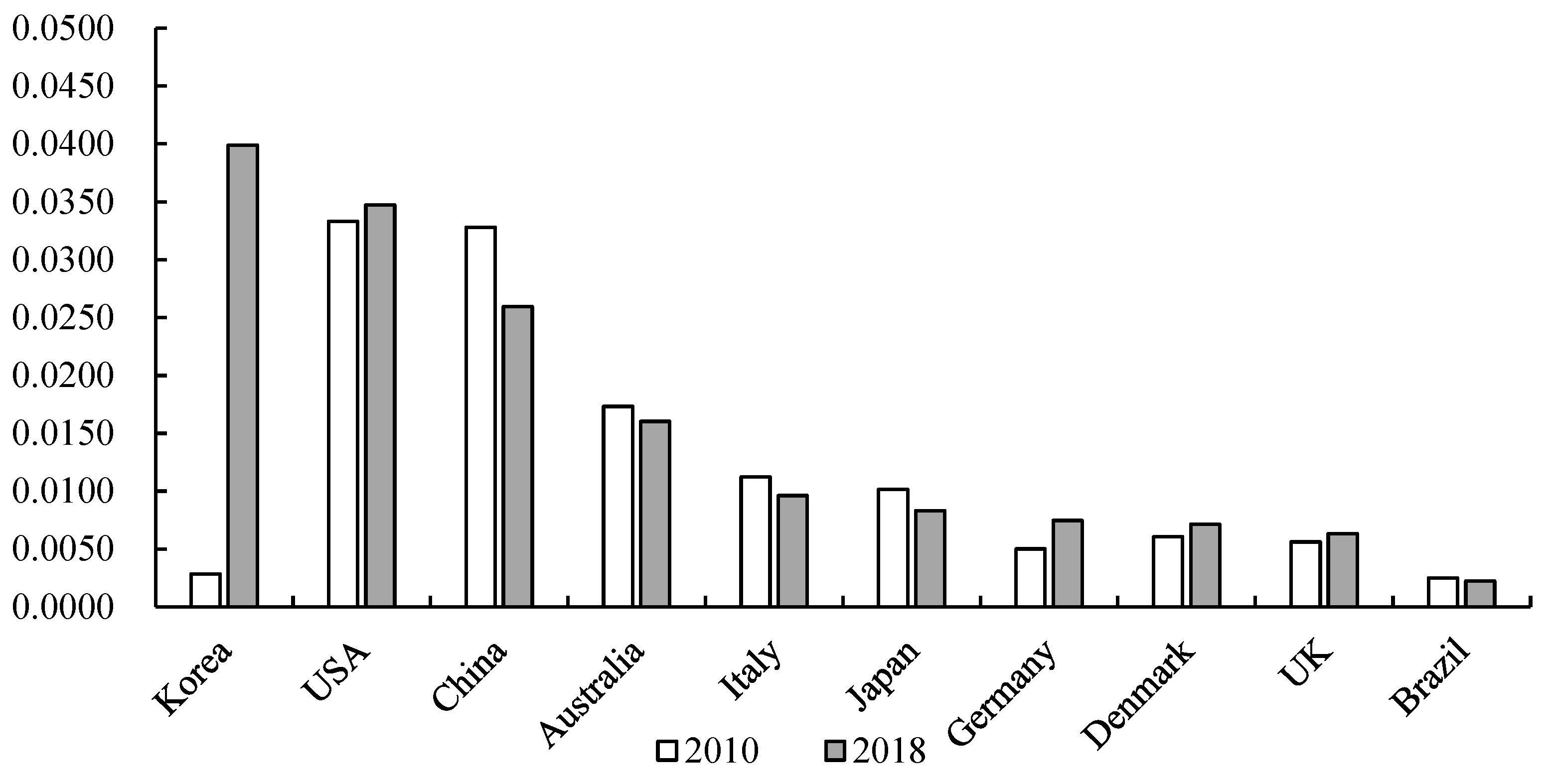
| 11 | Australia | D64T66 | 0.1407 | D64T66 | 0.1420 | D64T66 | 0.14179 |
| D41T43 | 0.0647 | D41T43 | 0.0549 | D41T43 | 0.05588 | ||
| 12 | Denmark | D41T43 | 0.0954 | D64T66 | 0.0991 | D41T43 | 0.10031 |
| D64T66 | 0.0933 | D41T43 | 0.0922 | D64T66 | 0.09122 | ||
| 13 | Spain | D64T66 | 0.0510 | D64T66 | 0.0359 | D64T66 | 0.03844 |
| D41T43 | 0.0350 | D41T43 | 0.0246 | D41T43 | 0.03707 | ||
| 14 | Vietnam | D35 | 0.0343 | D41T43 | 0.1045 | D41T43 | 0.15955 |
| D41T43 | 0.0190 | D23 | 0.0244 | D69T75 | 0.02405 | ||
| 15 | New Zealand | D64T66 | 0.0725 | D68 | 0.0700 | D68 | 0.06804 |
| D68 | 0.0626 | D64T66 | 0.0659 | D41T43 | 0.06309 | ||
| 16 | Brunei Darussalam | D64T66 | 0.0580 | D64T66 | 0.0558 | D64T66 | 0.08456 |
| D41T43 | 0.0441 | D41T43 | 0.0397 | D41T43 | 0.01507 | ||
| 17 | Malta | D41T43 | 0.0493 | D41T43 | 0.0654 | D41T43 | 0.06780 |
| D68 | 0.0459 | D69T75 | 0.0294 | D69T75 | 0.03204 | ||
| 18 | Poland | D35 | 0.1337 | D41T43 | 0.1055 | D35 | 0.11195 |
| D41T43 | 0.0950 | D35 | 0.0878 | D41T43 | 0.09533 | ||
| 19 | Malaysia | D64T66 | 0.1246 | D64T66 | 0.0507 | D19 | 0.05428 |
| D68 | 0.0670 | D41T43 | 0.0362 | D64T66 | 0.04909 | ||
| 20 | The Netherlands | D64T66 | 0.2525 | D64T66 | 0.2845 | D64T66 | 0.16119 |
| D41T43 | 0.0956 | D41T43 | 0.0947 | D41T43 | 0.11371 | ||
| 21 | Belgium | D41T43 | 0.0631 | D64T66 | 0.0726 | D64T66 | 0.06400 |
| D64T66 | 0.0573 | D41T43 | 0.0529 | D68 | 0.04031 | ||
| 22 | The Philippines | D64T66 | 0.0468 | D45T47 | 0.0510 | D45T47 | 0.04621 |
| D45T47 | 0.0257 | D01T02 | 0.0234 | D01T02 | 0.02126 | ||
| 23 | Latvia | D41T43 | 0.0882 | D68 | 0.0922 | D68 | 0.04967 |
| D35 | 0.0499 | D35 | 0.0336 | D35 | 0.02743 | ||
| 24 | Colombia | D64T66 | 0.0452 | D77T82 | 0.0264 | D77T82 | 0.02519 |
| D77T82 | 0.0216 | D41T43 | 0.0262 | D41T43 | 0.02253 | ||
| 25 | Saudi Arabia | D64T66 | 0.0307 | D41T43 | 0.0496 | D41T43 | 0.04495 |
| D41T43 | 0.0252 | D64T66 | 0.0118 | D64T66 | 0.00955 | ||
| 26 | France | D64T66 | 0.0642 | D64T66 | 0.0680 | D64T66 | 0.04581 |
| D68 | 0.0291 | D68 | 0.0241 | D68 | 0.02424 | ||
| 27 | Kazakhstan | D68 | 0.1183 | D41T43 | 0.0287 | D41T43 | 0.04484 |
| D01T02 | 0.0552 | D77T82 | 0.0154 | D49 | 0.02913 | ||
| 28 | Finland | D41T43 | 0.0614 | D41T43 | 0.0599 | D41T43 | 0.05633 |
| D64T66 | 0.0396 | D64T66 | 0.0394 | D64T66 | 0.04742 | ||
| 29 | Peru | D64T66 | 0.0389 | D64T66 | 0.0412 | D64T66 | 0.03190 |
| D69T75 | 0.0176 | D69T75 | 0.0172 | D69T75 | 0.01443 | ||
| 30 | China Non-Processing | D64T66 | 0.0430 | D64T66 | 0.0937 | D64T66 | 0.06999 |
| D77T82 | 0.0328 | D68 | 0.0390 | D77T82 | 0.02594 | ||
| 31 | Chinese Taipei | D64T66 | 0.0730 | D64T66 | 0.0700 | D41T43 | 0.05380 |
| D41T43 | 0.0480 | D41T43 | 0.0590 | D64T66 | 0.04865 | ||
| 32 | India | D41T43 | 0.0628 | D41T43 | 0.0675 | D41T43 | 0.06684 |
| D64T66 | 0.0221 | D64T66 | 0.0201 | D64T66 | 0.01887 | ||
| 33 | Myanmar | D64T66 | 0.1208 | D64T66 | 0.1250 | D64T66 | 0.12498 |
| D41T43 | 0.0506 | D41T43 | 0.0356 | D41T43 | 0.03231 | ||
| 34 | Iceland | D41T43 | 0.0600 | D41T43 | 0.0561 | D41T43 | 0.07944 |
| D64T66 | 0.0379 | D64T66 | 0.0383 | D64T66 | 0.03170 | ||
| 35 | Estonia | D41T43 | 0.0524 | D41T43 | 0.0552 | D41T43 | 0.08130 |
| D64T66 | 0.0506 | D64T66 | 0.0372 | D64T66 | 0.04036 | ||
| 36 | Luxembourg | D64T66 | 0.0656 | D64T66 | 0.0408 | D64T66 | 0.06971 |
| D41T43 | 0.0229 | D41T43 | 0.0280 | D41T43 | 0.04826 | ||
| 37 | The United States | D64T66 | 0.0530 | D64T66 | 0.0632 | D64T66 | 0.06276 |
| D68 | 0.0449 | D41T43 | 0.0435 | D41T43 | 0.04258 | ||
| 38 | Morocco | D64T66 | 0.0917 | D64T66 | 0.0938 | D64T66 | 0.08073 |
| D68 | 0.0035 | D69T75 | 0.0047 | D69T75 | 0.00357 | ||
| 39 | The Russian Federation | D68 | 0.0500 | D68 | 0.0414 | D68 | 0.05503 |
| D35 | 0.0293 | D35 | 0.0276 | D35 | 0.03533 | ||
| 40 | Ireland | D64T66 | 0.1764 | D64T66 | 0.0558 | D69T75 | 0.04008 |
| D41T43 | 0.0283 | D41T43 | 0.0174 | D41T43 | 0.02818 | ||
| 41 | Israel (2) | D64T66 | 0.0374 | D69T75 | 0.0274 | D69T75 | 0.03283 |
| D69T75 | 0.0355 | D64T66 | 0.0264 | D64T66 | 0.02481 | ||
| 42 | Chile | D41T43 | 0.1577 | D41T43 | 0.1185 | D41T43 | 0.10594 |
| D69T75 | 0.0268 | D64T66 | 0.0414 | D64T66 | 0.03776 | ||
| 43 | Germany | D41T43 | 0.0760 | D41T43 | 0.0709 | D41T43 | 0.07856 |
| D64T66 | 0.0556 | D64T66 | 0.0582 | D64T66 | 0.04656 | ||
| 44 | Bulgaria | D41T43 | 0.0727 | D64T66 | 0.0644 | D64T66 | 0.06928 |
| D64T66 | 0.0714 | D41T43 | 0.0558 | D41T43 | 0.06456 | ||
| 45 | Slovenia | D41T43 | 0.0331 | D41T43 | 0.0280 | D64T66 | 0.03400 |
| D64T66 | 0.0173 | D69T75 | 0.0167 | D41T43 | 0.02640 | ||
| 46 | Costa Rica | D64T66 | 0.0633 | D64T66 | 0.0527 | D64T66 | 0.05889 |
| D41T43 | 0.0350 | D41T43 | 0.0394 | D69T75 | 0.02724 | ||
| 47 | South Africa | D64T66 | 0.0441 | D64T66 | 0.0608 | D64T66 | 0.06020 |
| D45T47 | 0.0269 | D45T47 | 0.0266 | D45T47 | 0.02970 | ||
| 48 | Hungary | D64T66 | 0.0847 | D64T66 | 0.0655 | D64T66 | 0.05699 |
| D69T75 | 0.0271 | D41T43 | 0.0284 | D41T43 | 0.03587 | ||
| 49 | Norway | D64T66 | 0.0649 | D64T66 | 0.0871 | D64T66 | 0.06105 |
| D41T43 | 0.0460 | D41T43 | 0.0481 | D41T43 | 0.05338 | ||
| 50 | The United Kingdom | D64T66 | 0.1250 | D64T66 | 0.0858 | D64T66 | 0.06322 |
| D41T43 | 0.0631 | D41T43 | 0.0607 | D41T43 | 0.05257 | ||
| 51 | Cyprus (1) | D41T43 | 0.0993 | D41T43 | 0.0745 | D41T43 | 0.03609 |
| D64T66 | 0.0782 | D64T66 | 0.0482 | D68 | 0.01947 | ||
| 52 | Singapore | D64T66 | 0.0911 | D64T66 | 0.1046 | D64T66 | 0.08129 |
| D69T75 | 0.0489 | D69T75 | 0.0408 | D69T75 | 0.04449 | ||
| 53 | Korea | D64T66 | 0.0986 | D64T66 | 0.1253 | D64T66 | 0.10517 |
| D35 | 0.0211 | D41T43 | 0.0296 | D77T82 | 0.03990 | ||
| 54 | Italy | D64T66 | 0.0410 | D64T66 | 0.0339 | D64T66 | 0.02653 |
| D69T75 | 0.0289 | D69T75 | 0.0214 | D69T75 | 0.01574 | ||
| 55 | Rest of the World | D64T66 | 0.0390 | D64T66 | 0.0331 | D41T43 | 0.03980 |
| D41T43 | 0.0249 | D41T43 | 0.0255 | D64T66 | 0.03669 | ||
| 56 | Croatia | D45T47 | 0.0270 | D45T47 | 0.0239 | D41T43 | 0.05734 |
| D35 | 0.0210 | D35 | 0.0207 | D35 | 0.03070 | ||
| 57 | Canada | D64T66 | 0.0682 | D64T66 | 0.0687 | D64T66 | 0.06609 |
| D41T43 | 0.0538 | D41T43 | 0.0533 | D41T43 | 0.05844 | ||
| 58 | Hong Kong, China | D64T66 | 0.1227 | D64T66 | 0.1275 | D64T66 | 0.15151 |
| D68 | 0.0534 | D68 | 0.0572 | D68 | 0.05334 | ||
| 59 | Austria | D41T43 | 0.0848 | D41T43 | 0.0928 | D41T43 | 0.09489 |
| D36T39 | 0.0525 | D68 | 0.0451 | D68 | 0.05331 | ||
| 60 | Sweden | D41T43 | 0.1240 | D41T43 | 0.1311 | D41T43 | 0.12666 |
| D64T66 | 0.0615 | D64T66 | 0.0696 | D64T66 | 0.05518 | ||
| 61 | Mexico Non-global manufacturing | D68 | 0.0320 | D68 | 0.0399 | D68 | 0.02896 |
| D69T75 | 0.0137 | D69T75 | 0.0131 | D69T75 | 0.01084 | ||
| 62 | Portugal | D64T66 | 0.0390 | D64T66 | 0.0289 | D64T66 | 0.03465 |
| D41T43 | 0.0214 | D41T43 | 0.0197 | D41T43 | 0.01705 | ||
| 63 | Romania | D64T66 | 0.0312 | D64T66 | 0.0453 | D64T66 | 0.04394 |
| D41T43 | 0.0238 | D68 | 0.0188 | D68 | 0.02303 | ||
| 64 | Indonesia | D41T43 | 0.0799 | D41T43 | 0.0826 | D41T43 | 0.07438 |
| D64T66 | 0.0249 | D64T66 | 0.0187 | D64T66 | 0.01422 | ||
| 65 | Czechia | D41T43 | 0.0715 | D64T66 | 0.0778 | D41T43 | 0.07066 |
| D64T66 | 0.0706 | D41T43 | 0.0736 | D64T66 | 0.06289 | ||
| 66 | Lao (People’s Democratic Republic) | D41T43 | 0.1651 | D41T43 | 0.2114 | D41T43 | 0.24825 |
| D68 | 0.0241 | D68 | 0.0221 | D68 | 0.01296 | ||
| 67 | Brazil | D64T66 | 0.0513 | D64T66 | 0.0546 | D64T66 | 0.04594 |
| D41T43 | 0.0068 | D69T75 | 0.0065 | D69T75 | 0.00664 | ||
Appendix B. Direct Output Indicator of the Real Estate Sector from 2010 to 2018
| No. | Country/Region | 2010 | 2014 | 2018 | |||
| Sector | Value | Sector | Value | Sector | Value | ||
| 1 | Switzerland | D52 | 0.0324 | D61 | 0.0215 | D61 | 0.0214 |
| D55T56 | 0.0319 | D68 | 0.0209 | D68 | 0.0188 | ||
| 2 | Türkiye | D53 | 0.0557 | D53 | 0.0588 | D53 | 0.0638 |
| D45T47 | 0.0544 | D45T47 | 0.0533 | D45T47 | 0.0513 | ||
| 3 | Japan | D50 | 0.1083 | D50 | 0.1095 | D52 | 0.0413 |
| D52 | 0.0381 | D52 | 0.0416 | D68 | 0.0337 | ||
| 4 | Cambodia | D07T08 | 0.0278 | D68 | 0.0218 | D68 | 0.0255 |
| D16 | 0.0240 | D62T63 | 0.0157 | D62T63 | 0.0188 | ||
| 5 | Thailand | D64T66 | 0.0077 | D64T66 | 0.0072 | D58T60 | 0.0040 |
| D62T63 | 0.0053 | D58T60 | 0.0058 | D64T66 | 0.0036 | ||
| 6 | Tunisia | D90T93 | 0.0196 | D90T93 | 0.0158 | D90T93 | 0.0195 |
| D94T96 | 0.0157 | D94T96 | 0.0108 | D94T96 | 0.0110 | ||
| 7 | Greece | D61 | 0.2276 | D61 | 0.2426 | D61 | 0.2000 |
| D69T75 | 0.1440 | D45T47 | 0.1408 | D45T47 | 0.1139 | ||
| 8 | Argentina | D52 | 0.0335 | D52 | 0.0258 | D52 | 0.0229 |
| D45T47 | 0.0210 | D45T47 | 0.0164 | D45T47 | 0.0144 | ||
| 9 | Lithuania | D29 | 0.1159 | D68 | 0.0849 | D62T63 | 0.0676 |
| D03 | 0.1074 | D90T93 | 0.0658 | D90T93 | 0.0661 | ||
| 10 | Slovakia | D49 | 0.1338 | D55T56 | 0.0850 | D68 | 0.0739 |
| D55T56 | 0.0584 | D68 | 0.0571 | D90T93 | 0.0666 | ||
| 11 | Australia | D77T82 | 0.0427 | D77T82 | 0.0492 | D77T82 | 0.0541 |
| D45T47 | 0.0407 | D45T47 | 0.0451 | D45T47 | 0.0453 | ||
| 12 | Denmark | D55T56 | 0.0850 | D55T56 | 0.0881 | D55T56 | 0.0899 |
| D45T47 | 0.0743 | D45T47 | 0.0735 | D45T47 | 0.0663 | ||
| 13 | Spain | D45T47 | 0.0474 | D45T47 | 0.0462 | D45T47 | 0.0436 |
| D50 | 0.0401 | D50 | 0.0462 | D50 | 0.0390 | ||
| 14 | Vietnam | D53 | 0.0368 | D45T47 | 0.0228 | D45T47 | 0.0242 |
| D68 | 0.0179 | D68 | 0.0214 | D68 | 0.0231 | ||
| 15 | New Zealand | D52 | 0.0781 | D52 | 0.0777 | D52 | 0.0789 |
| D68 | 0.0626 | D68 | 0.0700 | D68 | 0.0680 | ||
| 16 | Brunei Darussalam | D90T93 | 0.0430 | D90T93 | 0.0376 | D90T93 | 0.0245 |
| D94T96 | 0.0171 | D94T96 | 0.0176 | D94T96 | 0.0105 | ||
| 17 | Malta | D68 | 0.0459 | D51 | 0.0188 | D51 | 0.0296 |
| D45T47 | 0.0237 | D45T47 | 0.0168 | D68 | 0.0283 | ||
| 18 | Poland | D90T93 | 0.0278 | D90T93 | 0.0272 | D90T93 | 0.0338 |
| D86T88 | 0.0210 | D86T88 | 0.0217 | D86T88 | 0.0326 | ||
| 19 | Malaysia | D68 | 0.0670 | D68 | 0.0267 | D68 | 0.0404 |
| D84 | 0.0332 | D84 | 0.0137 | D77T82 | 0.0153 | ||
| 20 | The Netherlands | D52 | 0.0585 | D52 | 0.0549 | D55T56 | 0.0448 |
| D55T56 | 0.0535 | D55T56 | 0.0433 | D52 | 0.0446 | ||
| 21 | Belgium | D52 | 0.0391 | D45T47 | 0.0338 | D68 | 0.0403 |
| D45T47 | 0.0371 | D52 | 0.0322 | D55T56 | 0.0393 | ||
| 22 | The Philippines | D51 | 0.0444 | D21 | 0.0165 | D21 | 0.0134 |
| D62T63 | 0.0338 | D07T08 | 0.0115 | D07T08 | 0.0095 | ||
| 23 | Latvia | D45T47 | 0.0744 | D55T56 | 0.1153 | D55T56 | 0.1316 |
| D90T93 | 0.0671 | D68 | 0.0922 | D45T47 | 0.0826 | ||
| 24 | Colombia | D45T47 | 0.0639 | D52 | 0.0659 | D52 | 0.0576 |
| D61 | 0.0549 | D45T47 | 0.0567 | D45T47 | 0.0531 | ||
| 25 | Saudi Arabia | D45T47 | 0.0231 | D45T47 | 0.0308 | D45T47 | 0.0307 |
| D31T33 | 0.0172 | D31T33 | 0.0280 | D31T33 | 0.0237 | ||
| 26 | France | D45T47 | 0.0458 | D45T47 | 0.0430 | D45T47 | 0.0418 |
| D77T82 | 0.0337 | D77T82 | 0.0318 | D77T82 | 0.0281 | ||
| 27 | Kazakhstan | D68 | 0.1183 | D94T96 | 0.2798 | D94T96 | 0.1683 |
| D10T12 | 0.0348 | D62T63 | 0.0511 | D64T66 | 0.1003 | ||
| 28 | Finland | D55T56 | 0.0719 | D55T56 | 0.0714 | D55T56 | 0.0654 |
| D51 | 0.0631 | D45T47 | 0.0608 | D45T47 | 0.0606 | ||
| 29 | Peru | D94T96 | 0.1018 | D94T96 | 0.0886 | D94T96 | 0.0850 |
| D85 | 0.0601 | D85 | 0.0494 | D61 | 0.0492 | ||
| 30 | China Non-Processing | D62T63 | 0.0341 | D45T47 | 0.0571 | D94T96 | 0.0624 |
| D61 | 0.0340 | D94T96 | 0.0405 | D45T47 | 0.0464 | ||
| 31 | Chinese Taipei | D90T93 | 0.0357 | D90T93 | 0.0399 | D55T56 | 0.0469 |
| D45T47 | 0.0335 | D45T47 | 0.0333 | D90T93 | 0.0415 | ||
| 32 | India | D41T43 | 0.0185 | D41T43 | 0.0223 | D49 | 0.0191 |
| D61 | 0.0128 | D49 | 0.0122 | D41T43 | 0.0185 | ||
| 33 | Myanmar | D68 | 0.0364 | D68 | 0.0302 | D68 | 0.0273 |
| D62T63 | 0.0255 | D62T63 | 0.0226 | D62T63 | 0.0254 | ||
| 34 | Iceland | D94T96 | 0.0274 | D94T96 | 0.0261 | D94T96 | 0.0258 |
| D68 | 0.0200 | D68 | 0.0220 | D68 | 0.0222 | ||
| 35 | Estonia | D55T56 | 0.0844 | D55T56 | 0.0936 | D55T56 | 0.1230 |
| D45T47 | 0.0721 | D45T47 | 0.0764 | D45T47 | 0.0882 | ||
| 36 | Luxembourg | D41T43 | 0.0594 | D77T82 | 0.0453 | D94T96 | 0.0354 |
| D77T82 | 0.0463 | D94T96 | 0.0349 | D77T82 | 0.0341 | ||
| 37 | The United States | D94T96 | 0.0847 | D94T96 | 0.0923 | D94T96 | 0.0826 |
| D90T93 | 0.0799 | D52 | 0.0776 | D55T56 | 0.0817 | ||
| 38 | Morocco | D52 | 0.0380 | D52 | 0.0292 | D52 | 0.0256 |
| D51 | 0.0291 | D58T60 | 0.0239 | D51 | 0.0237 | ||
| 39 | The Russian Federation | D94T96 | 0.0637 | D55T56 | 0.0589 | D55T56 | 0.0755 |
| D55T56 | 0.0606 | D49 | 0.0551 | D45T47 | 0.0573 | ||
| 40 | Ireland | D55T56 | 0.0675 | D55T56 | 0.0659 | D55T56 | 0.0729 |
| D45T47 | 0.0657 | D45T47 | 0.0404 | D90T93 | 0.0708 | ||
| 41 | Israel (2) | D52 | 0.0868 | D52 | 0.0804 | D55T56 | 0.0728 |
| D55T56 | 0.0668 | D55T56 | 0.0739 | D52 | 0.0709 | ||
| 42 | Chile | D55T56 | 0.0554 | D90T93 | 0.0617 | D61 | 0.0708 |
| D45T47 | 0.0548 | D45T47 | 0.0562 | D45T47 | 0.0648 | ||
| 43 | Germany | D61 | 0.0779 | D61 | 0.0703 | D61 | 0.0712 |
| D45T47 | 0.0766 | D55T56 | 0.0615 | D41T43 | 0.0569 | ||
| 44 | Bulgaria | D62T63 | 0.0733 | D62T63 | 0.0676 | D62T63 | 0.0650 |
| D61 | 0.0419 | D52 | 0.0524 | D52 | 0.0575 | ||
| 45 | Slovenia | D45T47 | 0.0215 | D36T39 | 0.0289 | D45T47 | 0.0109 |
| D52 | 0.0157 | D45T47 | 0.0208 | D55T56 | 0.0075 | ||
| 46 | Costa Rica | D35 | 0.0751 | D35 | 0.0648 | D35 | 0.0276 |
| D58T60 | 0.0521 | D58T60 | 0.0511 | D45T47 | 0.0155 | ||
| 47 | South Africa | D55T56 | 0.0452 | D45T47 | 0.0393 | D45T47 | 0.0423 |
| D45T47 | 0.0407 | D69T75 | 0.0327 | D69T75 | 0.0337 | ||
| 48 | Hungary | D90T93 | 0.0531 | D90T93 | 0.0563 | D94T96 | 0.0661 |
| D94T96 | 0.0492 | D94T96 | 0.0553 | D90T93 | 0.0525 | ||
| 49 | Norway | D55T56 | 0.0754 | D55T56 | 0.0759 | D55T56 | 0.0369 |
| D45T47 | 0.0632 | D45T47 | 0.0607 | D45T47 | 0.0367 | ||
| 50 | The United Kingdom | D45T47 | 0.0300 | D45T47 | 0.0340 | D45T47 | 0.0318 |
| D52 | 0.0183 | D52 | 0.0252 | D55T56 | 0.0229 | ||
| 51 | Cyprus (1) | D45T47 | 0.0599 | D45T47 | 0.0693 | D45T47 | 0.0436 |
| D58T60 | 0.0275 | D51 | 0.0359 | D53 | 0.0299 | ||
| 52 | Singapore | D94T96 | 0.0787 | D55T56 | 0.0916 | D55T56 | 0.0852 |
| D55T56 | 0.0541 | D94T96 | 0.0735 | D94T96 | 0.0661 | ||
| 53 | Korea | D55T56 | 0.0479 | D55T56 | 0.0473 | D45T47 | 0.0311 |
| D69T75 | 0.0334 | D69T75 | 0.0350 | D55T56 | 0.0273 | ||
| 54 | Italy | D45T47 | 0.0469 | D45T47 | 0.0476 | D55T56 | 0.0464 |
| D55T56 | 0.0425 | D55T56 | 0.0474 | D45T47 | 0.0462 | ||
| 55 | Rest of the World | D94T96 | 0.0293 | D94T96 | 0.0362 | D94T96 | 0.0374 |
| D55T56 | 0.0257 | D62T63 | 0.0243 | D55T56 | 0.0285 | ||
| 56 | Croatia | D45T47 | 0.0524 | D45T47 | 0.0487 | D53 | 0.0202 |
| D69T75 | 0.0264 | D53 | 0.0292 | D45T47 | 0.0198 | ||
| 57 | Canada | D94T96 | 0.0575 | D94T96 | 0.0525 | D94T96 | 0.0513 |
| D45T47 | 0.0375 | D45T47 | 0.0353 | D45T47 | 0.0364 | ||
| 58 | Hong Kong, China | D52 | 0.1338 | D94T96 | 0.1292 | D52 | 0.1329 |
| D94T96 | 0.1205 | D52 | 0.1175 | D94T96 | 0.1223 | ||
| 59 | Austria | D84 | 0.0475 | D50 | 0.0520 | D68 | 0.0533 |
| D68 | 0.0444 | D84 | 0.0458 | D84 | 0.0454 | ||
| 60 | Sweden | D55T56 | 0.0874 | D90T93 | 0.0883 | D84 | 0.0543 |
| D90T93 | 0.0846 | D85 | 0.0805 | D55T56 | 0.0521 | ||
| 61 | Mexico Non-global manufacturing | D52 | 0.0915 | D62T63 | 0.0871 | D58T60 | 0.0733 |
| D58T60 | 0.0644 | D58T60 | 0.0843 | D62T63 | 0.0722 | ||
| 62 | Portugal | D45T47 | 0.0295 | D45T47 | 0.0242 | D45T47 | 0.0161 |
| D53 | 0.0265 | D58T60 | 0.0224 | D90T93 | 0.0121 | ||
| 63 | Romania | D45T47 | 0.0591 | D45T47 | 0.0644 | D45T47 | 0.0561 |
| D68 | 0.0173 | D68 | 0.0188 | D68 | 0.0230 | ||
| 64 | Indonesia | D45T47 | 0.0223 | D94T96 | 0.0410 | D94T96 | 0.0366 |
| D62T63 | 0.0146 | D45T47 | 0.0176 | D45T47 | 0.0177 | ||
| 65 | Czechia | D90T93 | 0.0694 | D55T56 | 0.0754 | D55T56 | 0.0650 |
| D68 | 0.0670 | D68 | 0.0613 | D68 | 0.0601 | ||
| 66 | Lao (People’s Democratic Republic) | D85 | 0.0274 | D85 | 0.0390 | D85 | 0.0413 |
| D68 | 0.0241 | D45T47 | 0.0357 | D45T47 | 0.0366 | ||
| 67 | Brazil | D90T93 | 0.0948 | D90T93 | 0.1149 | D90T93 | 0.1267 |
| D45T47 | 0.0376 | D45T47 | 0.0417 | D45T47 | 0.0356 | ||
Appendix C. Pull and Push of the Real Estate Sector from 2000 to 2018
| Country/Region | 2010 | 2014 | 2018 | |||
| Pull Effects | Push Effects | Pull Effects | Push Effects | Pull Effects | Push Effects | |
| Argentina | 0.7240 | 0.6623 | 0.6816 | 0.6631 | 0.6547 | 0.6635 |
| Australia | 0.9719 | 0.8184 | 1.0419 | 0.8054 | 1.0618 | 0.7859 |
| Austria | 1.1660 | 0.9042 | 1.1861 | 0.9056 | 1.2188 | 0.9178 |
| Belgium | 1.0132 | 0.8483 | 0.9695 | 0.8234 | 1.0276 | 0.8090 |
| Bulgaria | 0.9174 | 0.7672 | 0.9977 | 0.7876 | 1.0568 | 0.8353 |
| Brazil | 0.9240 | 0.6356 | 0.9206 | 0.6250 | 0.9301 | 0.6222 |
| Brunei Darussalam | 0.5022 | 0.7342 | 0.5220 | 0.7348 | 0.4592 | 0.7285 |
| Canada | 0.9805 | 0.8403 | 0.9525 | 0.8397 | 0.9557 | 0.8463 |
| Switzerland | 0.8162 | 0.8396 | 0.6737 | 0.8081 | 0.6882 | 0.7892 |
| Chile | 1.0710 | 0.8509 | 1.0720 | 0.7890 | 1.1512 | 0.7836 |
| China | - | 0.6244 | - | 0.5958 | - | 0.5294 |
| Colombia | 1.1883 | 0.6829 | 1.1704 | 0.6653 | 1.1335 | 0.6571 |
| Costa Rica | 1.1362 | 0.8303 | 1.1558 | 0.8190 | 0.8336 | 0.8188 |
| Cyprus (1) | 0.8884 | 0.8841 | 0.9352 | 0.8466 | 0.9109 | 0.7485 |
| Czechia | 1.2871 | 0.9612 | 1.3162 | 0.9824 | 1.2969 | 0.9703 |
| Germany | 1.4208 | 0.8224 | 1.3567 | 0.8082 | 1.3347 | 0.8174 |
| Denmark | 1.3937 | 0.9189 | 1.3542 | 0.9289 | 1.3293 | 0.9474 |
| Spain | 0.9620 | 0.7005 | 0.9709 | 0.6764 | 1.0015 | 0.7139 |
| Estonia | 1.2085 | 0.8741 | 1.2922 | 0.8780 | 1.4380 | 0.8668 |
| Finland | 1.1814 | 0.8112 | 1.1845 | 0.8047 | 1.1778 | 0.8104 |
| France | 1.0367 | 0.7396 | 1.0105 | 0.7442 | 0.9911 | 0.7335 |
| The United Kingdom | 0.7914 | 0.8596 | 0.8386 | 0.8061 | 0.8452 | 0.7817 |
| Greece | 1.5648 | 0.7383 | 1.6828 | 0.7316 | 1.4925 | 0.7302 |
| Hong Kong, China | 0.4505 | 0.8196 | 0.5332 | 0.8367 | 0.6030 | 0.8488 |
| Croatia | 0.9750 | 0.7904 | 0.9846 | 0.8036 | 0.8205 | 0.9023 |
| Hungary | 1.2386 | 0.9210 | 1.1698 | 0.8934 | 1.2175 | 0.9288 |
| Indonesia | 0.6116 | 0.7217 | 0.6950 | 0.7446 | 0.6991 | 0.7179 |
| India | 0.5393 | 0.6819 | 0.5473 | 0.6816 | 0.5903 | 0.7047 |
| Ireland | 1.1166 | 0.9513 | 1.0432 | 0.8187 | 1.1893 | 0.8353 |
| Iceland | 0.8158 | 0.8300 | 0.8072 | 0.8408 | 0.8159 | 0.8775 |
| Israel (2) | 1.1326 | 0.7659 | 1.1742 | 0.7536 | 1.1770 | 0.7564 |
| Italy | 1.0799 | 0.6643 | 1.0952 | 0.6575 | 1.0822 | 0.6502 |
| Japan | 0.8948 | 0.6959 | 0.9192 | 0.7068 | 0.8988 | 0.7002 |
| Kazakhstan | 0.8641 | 0.9678 | 1.0446 | 0.7674 | 1.2353 | 0.8185 |
| Cambodia | 0.7380 | 0.9282 | 0.7609 | 0.9284 | 0.7544 | 0.9202 |
| Korea | 0.9414 | 0.6759 | 0.9523 | 0.7141 | 0.8518 | 0.7500 |
| Lao (People’s Democratic Republic) | 0.4533 | 0.8828 | 0.6445 | 0.8929 | 0.6454 | 0.8779 |
| Lithuania | 1.2074 | 0.8591 | 1.2568 | 0.9355 | 1.2912 | 0.9194 |
| Luxembourg | 1.1059 | 0.7891 | 0.9784 | 0.8082 | 1.1262 | 0.8615 |
| Latvia | 1.1303 | 0.8621 | 1.3012 | 0.7862 | 1.3313 | 0.7571 |
| Morocco | 0.9187 | 0.7590 | 0.9084 | 0.7834 | 0.9160 | 0.7853 |
| Malta | 0.9195 | 0.8613 | 0.8241 | 0.8655 | 0.8777 | 0.8828 |
| Myanmar | 0.3555 | 0.8344 | 0.3331 | 0.8319 | 0.3265 | 0.8345 |
| Malaysia | 0.6711 | 0.8398 | 0.6997 | 0.7757 | 0.6401 | 0.7854 |
| Mexico | - | 0.7027 | - | 0.7017 | - | 0.7185 |
| The Netherlands | 1.1446 | 1.0431 | 1.1010 | 1.0619 | 1.0343 | 1.0153 |
| Norway | 1.2357 | 0.8861 | 1.2243 | 0.8767 | 1.0253 | 0.8769 |
| New Zealand | 1.2664 | 0.8181 | 1.2788 | 0.8123 | 1.2875 | 0.8151 |
| Peru | 1.2119 | 0.7283 | 1.1519 | 0.7298 | 1.1563 | 0.7262 |
| The Philippines | 0.5193 | 0.7800 | 0.4080 | 0.7704 | 0.4187 | 0.7828 |
| Poland | 0.7483 | 0.9749 | 0.7945 | 0.9453 | 0.8514 | 0.9907 |
| Portugal | 0.8601 | 0.6919 | 0.8351 | 0.7042 | 0.7460 | 0.7131 |
| Romania | 0.6951 | 0.6807 | 0.7452 | 0.6975 | 0.7792 | 0.7538 |
| The Russian Federation | 1.0468 | 0.7470 | 1.0667 | 0.7453 | 1.1693 | 0.7629 |
| Saudi Arabia | 0.8141 | 0.7544 | 0.9364 | 0.7509 | 0.8299 | 0.7056 |
| Singapore | 1.0927 | 0.8953 | 1.0778 | 0.9012 | 1.0872 | 0.8989 |
| Slovakia | 1.3515 | 0.8647 | 1.2512 | 0.8913 | 1.1554 | 0.8685 |
| Slovenia | 0.8104 | 0.7506 | 0.8238 | 0.7644 | 0.6908 | 0.7736 |
| Sweden | 1.4561 | 0.9852 | 1.4617 | 0.9930 | 1.2941 | 0.9834 |
| Thailand | 0.5703 | 0.7515 | 0.5918 | 0.7529 | 0.5896 | 0.7186 |
| Tunisia | 0.8372 | 0.7640 | 0.8129 | 0.7739 | 0.8264 | 0.7791 |
| Türkiye | 0.9826 | 0.6149 | 0.9798 | 0.7426 | 1.0025 | 0.8446 |
| Chinese Taipei | 0.7439 | 0.7131 | 0.7925 | 0.7193 | 0.8504 | 0.7451 |
| The United States | 1.2636 | 0.8262 | 1.2679 | 0.8238 | 1.3262 | 0.8588 |
| Vietnam | 0.6766 | 0.7142 | 0.6655 | 0.7675 | 0.6155 | 0.8200 |
| South Africa | 1.1385 | 0.7319 | 1.0368 | 0.7878 | 1.0719 | 0.7947 |
| Rest of the World | 0.9078 | 0.7627 | 0.8858 | 0.7680 | 0.8917 | 0.7705 |
Appendix D
| No. | Classification | Sector | Change in Input Structure | Change in Output Structure | ||||||
| ↑ | ↓ | - | Total | ↑ | ↓ | - | Total | |||
| 1 | A | D01T02 | 23 | 23 | 25 | - | 37 | 21 | 13 | ↑ |
| 2 | D03 | 21 | 25 | 25 | ↓ | 17 | 11 | 43 | - | |
| 3 | B | D05T06 | 25 | 25 | 21 | ↑ | 25 | 22 | 24 | ↑ |
| 4 | D07T08 | 25 | 34 | 12 | ↓ | 30 | 18 | 23 | ↑ | |
| 5 | D09 | 26 | 31 | 14 | ↓ | 10 | 34 | 27 | ↓ | |
| 6 | C | D10T12 | 29 | 30 | 12 | ↓ | 35 | 27 | 9 | ↑ |
| 7 | D13T15 | 25 | 31 | 15 | ↓ | 27 | 26 | 18 | ↑ | |
| 8 | D16 | 31 | 27 | 13 | ↑ | 27 | 26 | 18 | ↑ | |
| 9 | D17T18 | 34 | 28 | 9 | ↑ | 22 | 39 | 10 | ↓ | |
| 10 | D19 | 24 | 25 | 22 | ↓ | 24 | 31 | 16 | ↓ | |
| 11 | D20 | 21 | 37 | 13 | ↓ | 24 | 36 | 11 | ↓ | |
| 12 | D21 | 28 | 25 | 18 | ↑ | 36 | 19 | 16 | ↑ | |
| 13 | D22 | 28 | 32 | 11 | ↓ | 31 | 28 | 12 | ↑ | |
| 14 | D23 | 29 | 26 | 16 | ↑ | 23 | 29 | 19 | ↓ | |
| 15 | D24 | 34 | 17 | 20 | ↑ | 27 | 31 | 13 | ↓ | |
| 16 | D25 | 36 | 26 | 9 | ↑ | 25 | 28 | 18 | ↓ | |
| 17 | D26 | 35 | 29 | 7 | ↑ | 30 | 34 | 7 | ↓ | |
| 18 | D27 | 29 | 29 | 13 | ↑ | 23 | 36 | 12 | ↓ | |
| 19 | D28 | 30 | 28 | 13 | ↑ | 25 | 25 | 21 | ↑ | |
| 20 | D29 | 27 | 30 | 14 | ↓ | 27 | 30 | 14 | ↓ | |
| 21 | D30 | 29 | 30 | 12 | ↓ | 29 | 20 | 22 | ↑ | |
| 22 | D31T33 | 29 | 33 | 9 | ↓ | 33 | 27 | 11 | ↑ | |
| 23 | D | D35 | 34 | 23 | 14 | ↑ | 24 | 18 | 29 | - |
| 24 | E | D36T39 | 36 | 24 | 11 | ↑ | 30 | 24 | 17 | ↑ |
| 25 | F | D41T43 | 30 | 25 | 16 | ↑ | 14 | 13 | 44 | - |
| 26 | G | D45T47 | 18 | 23 | 30 | - | 14 | 17 | 40 | - |
| 27 | D49 | 24 | 35 | 12 | ↓ | 27 | 29 | 15 | ↓ | |
| 28 | D50 | 23 | 34 | 14 | ↓ | 34 | 24 | 13 | ↑ | |
| 29 | D51 | 28 | 30 | 13 | ↓ | 37 | 22 | 12 | ↑ | |
| 30 | D52 | 21 | 34 | 16 | ↓ | 35 | 23 | 13 | ↑ | |
| 31 | D53 | 29 | 32 | 10 | ↓ | 28 | 29 | 14 | ↓ | |
| 32 | D55T56 | 31 | 21 | 19 | ↑ | 34 | 22 | 15 | ↑ | |
| 33 | D58T60 | 34 | 23 | 14 | ↑ | 22 | 37 | 12 | ↓ | |
| 34 | D61 | 32 | 26 | 13 | ↑ | 15 | 43 | 13 | ↓ | |
| 35 | D62T63 | 18 | 39 | 14 | ↓ | 45 | 14 | 12 | ↑ | |
| 36 | D64T66 | 33 | 25 | 13 | ↑ | 13 | 13 | 45 | - | |
| 37 | D68 | 24 | 31 | 16 | ↓ | 19 | 24 | 28 | - | |
| 38 | D69T75 | 26 | 27 | 18 | ↓ | 25 | 16 | 30 | - | |
| 39 | D77T82 | 19 | 31 | 21 | ↓ | 30 | 18 | 23 | ↑ | |
| 40 | D84 | 27 | 29 | 15 | ↓ | 28 | 25 | 18 | ↑ | |
| 41 | D85 | 25 | 30 | 16 | ↓ | 35 | 22 | 14 | ↑ | |
| 42 | D86T88 | 30 | 22 | 19 | ↑ | 31 | 25 | 15 | ↑ | |
| 43 | D90T93 | 23 | 30 | 18 | ↓ | 30 | 24 | 17 | ↑ | |
| 44 | D94T96 | 27 | 22 | 22 | ↑ | 24 | 30 | 17 | ↓ | |
| 45 | D97T98 | 0 | 0 | 71 | - | 0 | 0 | 71 | - | |
References
- Miller, N.; Peng, L.; Sklarz, M. House prices and economic growth. J. Real Estate Financ. Econ. 2011, 42, 522–541. [Google Scholar] [CrossRef]
- Jacob, B.A.; Ludwig, J. The effects of housing assistance on labor supply: Evidence from a voucher lottery. Am. Econ. Rev. 2012, 102, 272–304. [Google Scholar] [CrossRef]
- Strauss, J. Does housing drive state-level job growth? Building permits and consumer expectations forecast a state’s economic activity. J. Urban Econ. 2013, 73, 77–93. [Google Scholar] [CrossRef]
- Glaeser, E.; Gyourko, J. The economic implications of housing supply. J. Econ. Perspect. 2018, 32, 3–30. [Google Scholar] [CrossRef]
- Apergis, N. The role of housing market in the effectiveness of monetary policy over the COVID-19 era. Econ. Lett. 2021, 200, 109749. [Google Scholar] [CrossRef] [PubMed]
- Campbell, J.Y.; Cocco, J.F. How do house prices affect consumption? Evidence from micro data. J. Monet. Econ. 2007, 54, 591–621. [Google Scholar] [CrossRef]
- Glaeser, E.L.; Gottlieb, J.D.; Tobio, K. Housing booms and city centers. Am. Econ. Rev. 2012, 102, 127–133. [Google Scholar] [CrossRef]
- Iacoviello, M. House prices, borrowing constraints, and monetary policy in the business cycle. Am. Econ. Rev. 2005, 95, 739–764. [Google Scholar] [CrossRef]
- Squires, G.; Heurkens, E. Methods and models for international comparative approaches to real estate development. Land Use Policy 2016, 50, 573–581. [Google Scholar] [CrossRef]
- Chambers, M.; Garriga, C.; Schlagenhauf, D.E. Housing policy and the progressivity of income taxation. J. Monet. Econ. 2009, 56, 1116–1134. [Google Scholar] [CrossRef]
- Floetotto, M.; Kirker, M.; Stroebel, J. Government intervention in the housing market: Who wins, who loses? J. Monet. Econ. 2016, 80, 106–123. [Google Scholar] [CrossRef]
- Hoen, A.R. Identifying linkages with a cluster-based methodology. Econ. Syst. Res. 2002, 14, 131–146. [Google Scholar] [CrossRef]
- Leontief, W.W. Quantitative input and output relations in the economic systems of the United States. Rev. Econ. Stat. 1936, 18, 105–125. [Google Scholar] [CrossRef]
- Cai, J.; Leung, P. Linkage measures: A revisit and a suggested alternative. Econ. Syst. Res. 2004, 16, 63–83. [Google Scholar] [CrossRef]
- San Cristobal, J.R.; Biezma, M.V. The mining industry in the European Union: Analysis of inter-industry linkages using input–output analysis. Resour. Policy 2006, 31, 1–6. [Google Scholar] [CrossRef]
- Hauknes, J.; Knell, M. Embodied knowledge and sectoral linkages: An input–output approach to the interaction of high-and low-tech industries. Res. Policy 2009, 38, 459–469. [Google Scholar] [CrossRef]
- Yuan, R.; Behrens, P.; Rodrigues, J.F. The evolution of inter-sectoral linkages in China’s energy-related CO2 emissions from 1997 to 2012. Energy Econ. 2018, 69, 404–417. [Google Scholar] [CrossRef]
- Pagliari, J.; Webb, J.; Canter, T.; Frederich, S.S.R. A fundamental comparison of international real estate returns. J. Real Estate Res. 1997, 13, 317–347. [Google Scholar] [CrossRef]
- Song, Y.; Liu, C. An input–output approach for measuring real estate sector linkages. J. Prop. Res. 2007, 24, 71–91. [Google Scholar] [CrossRef]
- Bielsa, J.; Duarte, R. Size and linkages of the Spanish construction industry: Key sector or deformation of the economy? Camb. J. Econ. 2010, 35, 317–334. [Google Scholar] [CrossRef]
- Ren, H.; Folmer, H.; Van der Vlist, A.J. What role does the real estate–construction sector play in China’s regional economy? Ann. Reg. Sci. 2014, 52, 839–857. [Google Scholar] [CrossRef]
- Chan, S.; Han, G.; Zhang, W. How strong are the linkages between real estate and other sectors in China? Res. Int. Bus. Financ. 2016, 36, 52–72. [Google Scholar] [CrossRef]
- Liu, C.; Zhu, R. Measuring output structures of multinational construction industries using the World Input—Output Database. Int. J. Constr. Manag. 2017, 17, 1–12. [Google Scholar] [CrossRef]
- Weisz, H.; Duchin, F. Physical and monetary input–output analysis: What makes the difference? Ecol. Econ. 2006, 57, 534–541. [Google Scholar] [CrossRef]
- Rasmussen, P.N. Studies in Inter-Sectoral Relations; Einar Harck: Copenhagen, Denmark, 1956. [Google Scholar]
- Li, X.T.; Liu, F.; Wu, D.; Dong, J.C.; Gao, P. Exploring the role of the real estate sector in the Chinese economy: 1997–2007. Syst. Eng. Theory Pract. 2014, 14, 279–297. [Google Scholar]
- Liu, Q.Y. The research on the method of structural analyses regarding the input output coefficients. Stat. Res. 2002, 2, 40–42. [Google Scholar]
- OECD. STAN Input Output Database, OECD Inter-Country Input-Output (ICIO) Tables. Available online: https://www.oecd.org/sti/ind/inter-country-input-output-tables.htm (accessed on 28 April 2024).
- Hu, B.; McAleer, M. Input–output structure and growth in China. Math. Comput. Simul. 2004, 64, 193–202. [Google Scholar] [CrossRef]
- Lieser, K.; Groh, A.P. The determinants of international commercial real estate investment. J. Real Estate Financ. Econ. 2014, 48, 611–659. [Google Scholar] [CrossRef]
- Eichholtz, P.; Lindenthal, T. Demographics, human capital, and the demand for housing. J. Hous. Econ. 2014, 26, 19–32. [Google Scholar] [CrossRef]
- Wang, Z.; Zhang, Q. Fundamental factors in the housing markets of China. J. Hous. Econ. 2014, 25, 53–61. [Google Scholar] [CrossRef]
- Füss, R.; Zietz, J. The economic drivers of differences in house price inflation rates across MSAs. J. Hous. Econ. 2016, 31, 35–53. [Google Scholar] [CrossRef]
- Steegmans, J.; Hassink, W. Financial position and house price determination: An empirical study of income and wealth effects. J. Hous. Econ. 2017, 36, 8–24. [Google Scholar] [CrossRef]
- Cao, Y.; Chen, J.; Zhang, Q. Housing investment in urban China. J. Comp. Econ. 2018, 46, 212–247. [Google Scholar] [CrossRef]


| Rank | 2010 | 2014 | 2018 | |||
|---|---|---|---|---|---|---|
| Sector | Value | Sector | Value | Sector | Value | |
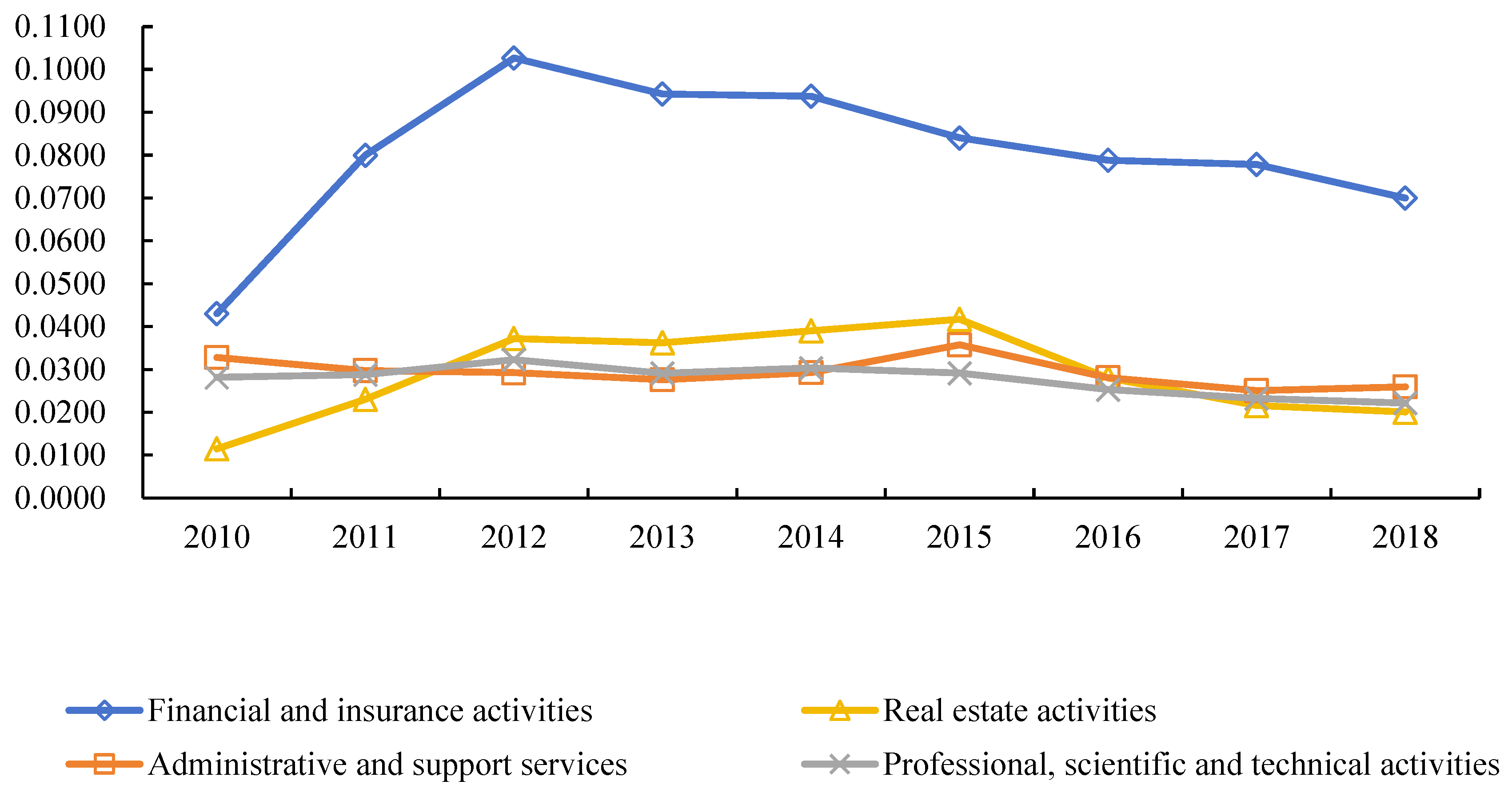
| 1 | Financial and insurance activities | 0.0430 | Financial and insurance activities | 0.0937 | Financial and insurance activities | 0.0700 |
| 2 | Administrative and support services | 0.0328 | Real estate activities | 0.0390 | Administrative and support services | 0.0259 |
| 3 | Professional, scientific, and technical activities | 0.0282 | Professional, scientific, and technical activities | 0.0303 | Professional, scientific, and technical activities | 0.0222 |
| 4 | Accommodation and food service activities | 0.0158 | Administrative and support services | 0.0293 | Real estate activities | 0.0201 |
| 5 | Construction | 0.0144 | Electricity, gas, steam, and air conditioning supply | 0.0268 | Construction | 0.0062 |
| Rank | 2010 | 2014 | 2018 | |||
|---|---|---|---|---|---|---|
| Sector | Value | Sector | Value | Sector | Value | |
| 1 | IT and other information services | 0.0341 | Wholesale and retail trade | 0.0571 | Other service activities | 0.0624 |
| 2 | Telecommunications | 0.0340 | Other service activities | 0.0405 | Wholesale and retail trade | 0.0464 |
| 3 | Other service activities | 0.0236 | Real estate activities | 0.0390 | IT and other information services | 0.0335 |
| 4 | Professional, scientific, and technical activities | 0.0177 | Financial and insurance activities | 0.0305 | Postal and courier activities | 0.0320 |
| 5 | Wholesale and retail trade | 0.0150 | Telecommunications | 0.0241 | Professional, scientific, and technical activities | 0.0306 |
| Classification | A | B | C | D | E | F | G | |
|---|---|---|---|---|---|---|---|---|
| Trend | ||||||||
| Input structure | uptrend | 0 | 1 | 9 | 1 | 1 | 1 | 6 |
| downtrend | 1 | 2 | 8 | 0 | 0 | 0 | 12 | |
| unchanging | 1 | 0 | 0 | 0 | 0 | 0 | 2 | |
| Output structure | uptrend | 1 | 2 | 8 | 0 | 1 | 0 | 10 |
| downtrend | 0 | 1 | 9 | 0 | 0 | 0 | 6 | |
| unchanging | 1 | 0 | 0 | 1 | 0 | 1 | 4 |
| Country/Region | Pull Effects | Push Effects | ||
|---|---|---|---|---|
| 2010 | 2018 | 2010 | 2018 | |
| UK | 34 | 32 (↑) | 13 | 24 (↓) |
| Denmark | 4 | 5 (↓) | 7 | 5 (↑) |
| Germany | 3 | 3 (-) | 19 | 19 (-) |
| Korea | 27 | 29 (↓) | 36 | 29 (↑) |
| China | - | - | 39 | 40 (↓) |
| Japan | 30 | 28 (↑) | 32 | 37 (↓) |
| Italy | 18 | 17 (↑) | 37 | 38 (↓) |
| Australia | 25 | 18 (↑) | 20 | 23 (↓) |
| Brazil | 28 | 27 (↑) | 38 | 39 (↓) |
| USA | 7 | 6 (↑) | 18 | 14 (↑) |
| Variables | Specification |
|---|---|
| Push | The push effects of the real estate sector in the economy (ISD) |
| Pull | The pull effects of the real estate sector in the economy (IPD) |
| Gdpy | The annual growth of GDP |
| Lnpgdp | The logarithm of real gross domestic product (GDP) per capita |
| Industry | The share of industry value added to GDP |
| Investratio | The ratio of fixed capital formation to final consumption, namely fixed capital formation divided by final consumption |
| Private | The share of domestic credit to the private sector in GDP |
| Stock | The share of the total value of stocks traded in GDP |
| Urbanization | The share of the urban population in the total population |
| Oldratio | The elderly dependency ratio, i.e., population ages 65 and above divided by population ages 15–64. |
| Variables | Mean | Median | Maximum | Minimum | Std. Dev. | Unit of Measurement |
|---|---|---|---|---|---|---|
| Push | 0.973 | 0.986 | 1.683 | 0.305 | 0.263 | - |
| Pull | 0.806 | 0.804 | 1.085 | 0.615 | 0.0890 | - |
| Gdpy | 3.090 | 2.779 | 24.48 | −10.15 | 2.908 | % |
| Pgdp | 26.33 | 26.41 | 30.65 | 22.69 | 1.618 | US$ Current Price |
| Industry | 2633 | 2519 | 7367 | 647.9 | 935.5 | % of GDP |
| Investratio | 0.359 | 0.325 | 1.176 | 0.142 | 0.141 | - |
| Private | 89.13 | 69.75 | 524.5 | 4.767 | 68.33 | % of GDP |
| Stock | 44.81 | 14.66 | 668.6 | 0.0100 | 86.41 | % of GDP |
| Urbanization | 71.63 | 74.43 | 100 | 20.29 | 17.92 | % |
| Oldratio | 19.97 | 20.59 | 49.10 | 3.132 | 9.077 | % |
| Variables | Pull | Push | Gdpy | Lnpgdp | Industry | Investratio | Private | Stock | Urbanization | Oldratio |
|---|---|---|---|---|---|---|---|---|---|---|
| Pull | 1 | |||||||||
| Push | 0.272 *** | 1 | ||||||||
| Gdpy | 0.087 ** | −0.296 *** | 1 | |||||||
| Lnpgdp | −0.272 *** | 0.144 *** | −0.140 *** | 1 | ||||||
| Industry | −0.154 *** | −0.320 *** | 0.213 *** | −0.0360 | 1 | |||||
| Investratio | 0.071 * | −0.245 *** | 0.241 *** | −0.145 *** | 0.486 *** | 1 | ||||
| Private | 0.138 *** | 0.0570 | −0.260 *** | −0.0290 | −0.356 *** | −0.127 *** | 1 | |||
| Stock | 0.0540 | −0.175 *** | 0.000 | 0.242 *** | −0.222 *** | 0.126 *** | 0.209 *** | 1 | ||
| Urbanization | 0.0170 | 0.413 *** | −0.320 *** | 0.272 *** | −0.314 *** | 0.0250 | 0.146 *** | 0.254 *** | 1 | |
| Oldratio | 0.178 *** | 0.498 *** | −0.408 *** | 0.200 *** | −0.478 *** | −0.321 *** | 0.303 *** | 0.0680 | 0.374 *** | 1 |
| Variables | (1) | (2) |
|---|---|---|
| Pull | Pull | |
| Gdpy | 0.477 *** | 0.504 *** |
| (0.139) | (0.144) | |
| Lnpgdp | −1.664 *** | −1.666 *** |
| (0.245) | (0.247) | |
| Industry | −0.000907 * | −0.000931 * |
| (0.000527) | (0.000532) | |
| Investratio | 8.299 *** | 8.420 *** |
| (3.171) | (3.213) | |
| Oldratio | 0.283 *** | 0.292 *** |
| (0.0490) | (0.0501) | |
| Private | 0.00737 | 0.00705 |
| (0.00583) | (0.00588) | |
| Stock | 0.00660 | 0.00660 |
| (0.00532) | (0.00537) | |
| Urbanization | −0.00179 | −0.00152 |
| (0.0241) | (0.0242) | |
| Constant | 115.7 *** | 115.5 *** |
| (6.551) | (6.604) | |
| Time | No | Yes |
| Observations | 545 | 545 |
| R-squared | 0.180 | 0.182 |
| Number of ID | 63 | 63 |
| Variables | (1) | (2) |
|---|---|---|
| Push | Push | |
| Industry | −0.00361 *** | −0.00379 *** |
| (0.00132) | (0.00133) | |
| Private | −0.0340 ** | −0.0359 ** |
| (0.0146) | (0.0147) | |
| Stock | −0.101 *** | −0.102 *** |
| (0.0133) | (0.0134) | |
| Urbanization | 0.455 *** | 0.452 *** |
| (0.0603) | (0.0606) | |
| Oldratio | 0.964 *** | 0.993 *** |
| (0.123) | (0.125) | |
| Gdpy | −0.386 | −0.395 |
| (0.348) | (0.360) | |
| Lnpgdp | 0.894 | 0.936 |
| (0.615) | (0.619) | |
| Investratio | −7.572 | −6.001 |
| (7.947) | (8.038) | |
| Constant | 42.94 *** | 41.72 ** |
| (16.42) | (16.52) | |
| Time | No | Yes |
| Observations | 545 | 545 |
| R-squared | 0.327 | 0.400 |
| Number of ID | 63 | 63 |
| Variables | (1) | (2) |
|---|---|---|
| Pull | Pull | |
| L.gdpy | 0.444 *** | 0.465 *** |
| (0.142) | (0.147) | |
| L.lnpgdp | −1.712 *** | −1.714 *** |
| (0.256) | (0.258) | |
| L.industry | −0.00101 * | −0.00103 * |
| (0.000546) | (0.000552) | |
| L.investratio | 8.689 ** | 8.765 ** |
| (3.379) | (3.420) | |
| L.oldratio | 0.295 *** | 0.302 *** |
| (0.0524) | (0.0533) | |
| L.private | 0.00512 | 0.00494 |
| (0.00602) | (0.00607) | |
| L.stock | 0.00832 | 0.00833 |
| (0.00566) | (0.00571) | |
| L.urbanization | −0.00731 | −0.00702 |
| (0.0249) | (0.0251) | |
| Constant | 117.6 *** | 117.4 *** |
| (6.817) | (6.871) | |
| Observations | 486 | 486 |
| R-squared | 0.188 | 0.189 |
| Number of ID | 63 | 63 |
| Variables | (1) | (2) |
|---|---|---|
| Push | Push | |
| L.industry | −0.00356 ** | −0.00374 *** |
| (0.00139) | (0.00140) | |
| L.private | −0.0377 ** | −0.0394 ** |
| (0.0153) | (0.0154) | |
| L.stock | −0.0981 *** | −0.0994 *** |
| (0.0144) | (0.0145) | |
| L.urbanization | 0.446 *** | 0.443 *** |
| (0.0635) | (0.0638) | |
| L.oldratio | 0.992 *** | 1.015 *** |
| (0.134) | (0.136) | |
| L.gdpy | −0.416 | −0.440 |
| (0.361) | (0.373) | |
| L.lnpgdp | 0.879 | 0.916 |
| (0.653) | (0.657) | |
| L.investratio | −5.731 | −4.340 |
| (8.609) | (8.693) | |
| Constant | 43.26 ** | 42.32 ** |
| (17.37) | (17.47) | |
| Time | No | Yes |
| Observations | 486 | 486 |
| R-squared | 0.390 | 0.394 |
| Number of ID | 63 | 63 |
| Variables | (1) | (2) | (3) | (4) |
|---|---|---|---|---|
| Pull | Pull | Pull | Pull | |
| Gdpy | 0.477 *** | 0.504 *** | 0.475 *** | 0.502 *** |
| (0.139) | (0.144) | (0.130) | (0.135) | |
| Lnpgdp | −1.664 *** | −1.666 *** | −1.604 *** | −1.603 *** |
| (0.245) | (0.247) | (0.219) | (0.220) | |
| Industry | −0.000907 * | −0.000931 * | −0.00128 *** | −0.00129 *** |
| (0.000527) | (0.000532) | (0.000459) | (0.000461) | |
| Investratio | 8.299 *** | 8.420 *** | 9.350 *** | 9.491 *** |
| (3.171) | (3.213) | (2.838) | (2.865) | |
| Oldratio | 0.283 *** | 0.292 *** | 0.279 *** | 0.288 *** |
| (0.0490) | (0.0501) | (0.0468) | (0.0477) | |
| Private | 0.00737 | 0.00705 | ||
| (0.00583) | (0.00588) | |||
| Stock | 0.00660 | 0.00660 | ||
| (0.00532) | (0.00537) | |||
| Urbanization | −0.00179 | −0.00152 | ||
| (0.0241) | (0.0242) | |||
| Constant | 115.7 *** | 115.5 *** | 115.8 *** | 115.5 *** |
| (6.551) | (6.604) | (5.938) | (5.985) | |
| Control variables | Yes | Yes | No | No |
| Time | No | Yes | No | Yes |
| Observations | 545 | 545 | 545 | 545 |
| R-squared | 0.180 | 0.182 | 0.174 | 0.176 |
| Number of ID | 63 | 63 | 63 | 63 |
| Variables | (1) | (2) | (3) | (4) |
|---|---|---|---|---|
| Push | Push | Push | Push | |
| Industry | −0.00361 *** | −0.00379 *** | −0.00399 *** | −0.00405 *** |
| (0.00132) | (0.00133) | (0.00113) | (0.00114) | |
| Private | −0.0340 ** | −0.0359 ** | −0.0341 ** | −0.0363 ** |
| (0.0146) | (0.0147) | (0.0143) | (0.0144) | |
| Stock | −0.101 *** | −0.102 *** | −0.101 *** | −0.101 *** |
| (0.0133) | (0.0134) | (0.0125) | (0.0125) | |
| Urbanization | 0.455 *** | 0.452 *** | 0.467 *** | 0.466 *** |
| (0.0603) | (0.0606) | (0.0563) | (0.0566) | |
| Oldratio | 0.964 *** | 0.993 *** | 1.050 *** | 1.080 *** |
| (0.123) | (0.125) | (0.117) | (0.119) | |
| Gdpy | −0.386 | −0.395 | ||
| (0.348) | (0.360) | |||
| Lnpgdp | 0.894 | 0.936 | ||
| (0.615) | (0.619) | |||
| Investratio | −7.572 | −6.001 | ||
| (7.947) | (8.038) | |||
| Constant | 42.94 *** | 41.72 ** | 61.05 *** | 60.85 *** |
| (16.42) | (16.52) | (6.136) | (6.163) | |
| Control variables | Yes | Yes | No | No |
| Time | No | Yes | No | Yes |
| Observations | 545 | 545 | 545 | 545 |
| R-squared | 0.327 | 0.400 | 0.389 | 0.394 |
| Number of ID | 63 | 63 | 63 | 63 |
| Variables | (1) Low Government Regulation | (2) High Government Regulation |
|---|---|---|
| Pull | Pull | |
| Gdpy | 0.540 ** | 0.259 |
| (0.242) | (0.236) | |
| Lnpgdp | −0.733 ** | −1.374 *** |
| (0.363) | (0.424) | |
| Industry | −0.00416 *** | 0.00119 |
| (0.00122) | (0.000849) | |
| Investratio | 19.09 ** | 16.07 *** |
| (8.330) | (4.772) | |
| Oldratio | 0.178 ** | 0.498 *** |
| (0.0879) | (0.0881) | |
| Private | 0.0108 | −0.00223 |
| (0.0150) | (0.00627) | |
| Stock | −0.0135 * | −0.00869 |
| (0.00803) | (0.0289) | |
| Urbanization | −0.0164 | −0.137 ** |
| (0.0396) | (0.0567) | |
| Constant | 100.0 *** | 105.9 *** |
| (9.685) | (11.92) | |
| Time | Yes | Yes |
| Observations | 170 | 0.259 |
| R-squared | 0.244 | (0.236) |
| Variables | (1) Low Government Regulation | (2) High Government Regulation |
|---|---|---|
| Push | Push | |
| Industry | −0.0177 *** | −0.00280 |
| (0.00390) | (0.00199) | |
| Private | −0.195 *** | 0.000766 |
| (0.0482) | (0.0147) | |
| Stock | −0.148 *** | 0.0904 |
| (0.0258) | (0.0679) | |
| Urbanization | 0.398 *** | 0.150 |
| (0.127) | (0.133) | |
| Oldratio | 1.124 *** | 0.387 * |
| (0.282) | (0.207) | |
| Gdpy | −2.616 *** | 1.170 ** |
| (0.776) | (0.554) | |
| Lnpgdp | 3.107 *** | −2.628 *** |
| (1.164) | (0.994) | |
| Investratio | 46.19 * | 8.801 |
| (26.72) | (11.19) | |
| Constant | 28.67 | 150.6 *** |
| (31.07) | (27.96) | |
| Time | Yes | Yes |
| Observations | 170 | 186 |
| R-squared | 0.673 | 0.157 |
| Variables | (1) Low Real Estate Development | (2) High Real Estate Development |
|---|---|---|
| Pull | Pull | |
| Gdpy | 0.579 * | 0.0480 |
| (0.313) | (0.238) | |
| Lnpgdp | −2.199 *** | −1.374 *** |
| (0.584) | (0.430) | |
| Industry | −0.00131 | 0.00338 ** |
| (0.00148) | (0.00143) | |
| Investratio | 16.03 | 3.680 |
| (11.60) | (4.171) | |
| Oldratio | 0.246 ** | 0.300 *** |
| (0.101) | (0.103) | |
| Private | 0.0959 *** | 0.00512 |
| (0.0292) | (0.00999) | |
| Stock | −0.0539 * | 0.0108 * |
| (0.0312) | (0.00641) | |
| Urbanization | −0.0119 | 0.155 *** |
| (0.0538) | (0.0544) | |
| Constant | 127.6 *** | 90.57 *** |
| (13.22) | (11.40) | |
| Time | Yes | Yes |
| Observations | 188 | 178 |
| R-squared | 0.223 | 0.212 |
| Variables | (1) Low Real Estate Development | (3) High Real Estate Development |
|---|---|---|
| Push | Push | |
| Industry | −0.0143 *** | −0.00115 |
| (0.00286) | (0.00345) | |
| Private | 0.204 *** | 0.0175 |
| (0.0565) | (0.0241) | |
| Stock | −0.248 *** | −0.101 *** |
| (0.0603) | (0.0155) | |
| Urbanization | 1.009 *** | 0.510 *** |
| (0.104) | (0.131) | |
| Oldratio | 0.452 ** | 0.0350 |
| (0.196) | (0.249) | |
| Gdpy | 0.167 | −0.641 |
| (0.604) | (0.574) | |
| Lnpgdp | −5.542 *** | 5.250 *** |
| (1.130) | (1.039) | |
| Investratio | 94.00 *** | 15.46 |
| (22.44) | (10.07) | |
| Constant | 173.5 *** | −81.59 *** |
| (25.57) | (27.52) | |
| Time | Yes | Yes |
| Observations | 188 | 178 |
| R-squared | 0.674 | 0.377 |
Disclaimer/Publisher’s Note: The statements, opinions and data contained in all publications are solely those of the individual author(s) and contributor(s) and not of MDPI and/or the editor(s). MDPI and/or the editor(s) disclaim responsibility for any injury to people or property resulting from any ideas, methods, instructions or products referred to in the content. |
© 2024 by the authors. Licensee MDPI, Basel, Switzerland. This article is an open access article distributed under the terms and conditions of the Creative Commons Attribution (CC BY) license (https://creativecommons.org/licenses/by/4.0/).
Share and Cite
Gao, W.; Wei, S.; Geng, C.; He, J.; Li, X.; Liu, S. The Role of the Real Estate Sector in the Economy: Cross-National Disparities and Their Determinants. Sustainability 2024, 16, 7697. https://doi.org/10.3390/su16177697
Gao W, Wei S, Geng C, He J, Li X, Liu S. The Role of the Real Estate Sector in the Economy: Cross-National Disparities and Their Determinants. Sustainability. 2024; 16(17):7697. https://doi.org/10.3390/su16177697
Chicago/Turabian StyleGao, Wei, Shan Wei, Chen Geng, Jing He, Xiuting Li, and Shuqin Liu. 2024. "The Role of the Real Estate Sector in the Economy: Cross-National Disparities and Their Determinants" Sustainability 16, no. 17: 7697. https://doi.org/10.3390/su16177697