Abstract
Geological reservoirs are widely used for storing or disposing of various fluids and gases, including groundwater, wastewater, carbon dioxide, air, gas, and hydrogen. Monitoring these sites is essential due to the stored assets’ economic value and the disposed materials’ hazardous nature. Reservoir pressure monitoring is vital for ensuring operational success and detecting integrity issues, but it presents challenges due to the difficulty of obtaining comprehensive pressure distribution data. While direct pressure measurement methods are costly and localized, indirect techniques offer a viable alternative, such as inferring reservoir pressure from surface deformation data. This inversion approach integrates a forward model that links pressure distribution to deformation with an optimization algorithm to account for the ill-posed nature of the inversion. The application of forward models for predicting subsidence, uplift, and seismicity is well-established, but using deformation data for monitoring underground activity through inversion has yet to be explored. Previous studies have used various analytical, semi-analytical, and numerical models integrated with optimization tools to perform efficient inversions. However, analytical or semi-analytical solutions are impractical for complex reservoirs, and advanced numerical models are computationally expensive. These studies often rely on prior information, which may only sometimes be available, highlighting the need for innovative approaches. This study addresses these challenges by leveraging advanced numerical models and genetic algorithms to estimate pressure distribution from surface deformation data without needing prior information. The forward model is based on a discrete Green matrix constructed by integrating the finite element method with Python scripting. This matrix encapsulates the influence of reservoir properties and geometry on the displacement field, allowing for the rapid evaluation of displacement due to arbitrary pressure distributions. Precomputing Green’s matrix reduces computational load, making it feasible to apply advanced optimization methods like GA, which are effective for solving ill-posed problems with fewer observation points than unknown parameters. Testing on complex reservoir cases with synthetic data showed less than 5% error in predicted pressure distribution, demonstrating the approach’s reliability.
1. Introduction
With the increasing demand for energy and the pressing need to mitigate climate change, geological reservoirs are increasingly being utilized as large and secure storage sites for energy or the disposal of hazardous fluids and gases. These reservoirs are commonly used for storing or disposing of groundwater, wastewater, carbon dioxide, air, gas, and hydrogen [1,2,3,4,5,6,7,8]. Reservoir pressure monitoring is a crucial parameter for the success and sustainable development of geological reservoirs; however, it presents significant challenges. Directly measuring reservoir pressure and its distribution is not easy [9,10]. The pressure measured at the wellhead, influenced by production systems and nearby formation permeability, does not accurately reflect overall reservoir pressure. In the exploration phase, seismic data are a valuable technique for reservoir pressure assessment [11]. Different approaches for pressure estimation from seismic data are available, including the Eaton method [12], the empirical formula method, the ratio method, and the Fillippone method [13]. However, these methods measure static pressure and cannot estimate dynamic pressure during injection and production phases [14]. The standard method for monitoring dynamic reservoir pressure typically relies on well-test data or bottom-hole gauges. However, the high cost of drilling limits data collection to a few wells, leading to significant uncertainties in predicting reservoir pressure distribution [15,16,17]. Accurately determining reservoir pressure across various locations requires an extensive and prolonged pressure recovery test to capture the pressure distribution throughout the entire reservoir block over different times, as the average formation pressure measured during a test reflects only a limited portion.
Alternatively, indirect monitoring techniques can be used to infer geological reservoir pressure. One such method is surface deformation inversion, which estimates pressure distribution within the reservoir. In addition, deformation data can provide vital information about the magnitude and extent of other subsurface activities. In hydraulic fracturing, these data are a diagnostic tool to assess fracture geometry and propagation [18]. Furthermore, it provides an indirect means of measuring the magnitude of fault slippage during fault reactivation or seismic activity [19].
A comprehensive literature review indicates that deformation and seismicity from geological storage or production pose significant risks to infrastructure and safety due to potential well and reservoir integrity issues, such as subsidence, wellbore instability, fault reactivation, and micro-seismicity. As a result, forward models predicting deformation from pressure disturbances in geological reservoirs have been extensively researched [20,21,22,23,24,25,26]. However, the inverse problem of using deformation data to infer pressure distribution in geological reservoirs has been studied less, and the inversion process is more complex. This complexity arises from the ill-posed nature of the problem, where the number of observational data points is significantly fewer than the unknowns, leading to substantial uncertainties. An optimization algorithm is necessary to address these uncertainties and minimize the cost function, representing the difference between the observed data and the data predicted by the forward model. Common types of cost functions include penalty function methods that use regularization techniques with smoothness or a priori model constraints to effectively manage the complexities of this ill-posed inverse problem [27,28,29,30,31].
Reviewing the studies that focused on mapping pressure distribution through deformation inversion, the forward models are generally classified into numerical and analytical/semi-analytical. The analytical approach is rooted in Kelvin’s development of a single force nucleus of strain in a full space [32,33]. Building on Kelvin’s work, Mindlin and Cheng (1936, 1950) expanded this concept to various sets of nuclei of strain based on different load types, applicable to both full-space and half-space scenarios. A significant contribution from Mindlin and Cheng (1936, 1950) for a half space was the center of dilatation [34,35]. Geertsma (1973) and Segall (1992) further derive an analytical solution for calculating the resultant displacement from a circular-shaped reservoir in an infinite medium, achieved by integrating the center of dilatation nucleus of strain over the volume of the cylindrical reservoir [36,37,38]. Following the approach of Geertsma (1973) and Segall (1992), semi-analytical solutions attempted to numerically integrate the center of dilatation nucleus of strain over the specific geometry of the problem [30]. Numerical forward modeling of reservoir compaction and surface subsidence typically employs the finite element method (FEM). Unlike analytical and semi-analytical methods, the finite element method (FEM) offers versatility in handling complex material behaviors, intricate reservoir geometries, and inhomogeneous conditions, albeit with increased computational costs [39,40,41,42,43,44,45,46,47,48].
The application of analytical forward models for real reservoir monitoring is rare since the analytical solutions are not representative of real and complex reservoir cases. Lee et al. (2023) explored the connection between surface displacement and underlying fault movement along with reservoir compaction or inflation by inversely solving elastic dislocation [19,49] and poroelastic compaction analytical solutions [36] using the penalty cost function [30] with priori information from seismic data [50].
Du and Olson (2001) used the semi-analytical forward model following the Segall (1992) approach to construct the discrete Green matrix. For the inversion approach, they applied the least square difference to minimize the penalty cost function (with a smoothness constraint and with priori information) [30]. They first developed this inversion approach for continuous mapping of opening displacement over a subsurface fracture plane and then applied their approach for pore pressure estimation [31]. Semi-analytical solutions can deal with irregularly shaped reservoirs but still involve several simplifications. One essential simplification is the assumption that the reservoir and surrounding layers share the same geomechanical properties, as reflected in the nucleus of the strain used. Additionally, semi-analytical solutions often perform integration over small, regularly shaped elements. However, accurately covering an irregularly shaped reservoir with these regular elements can be challenging and may not fully capture the reservoir’s true geometry.
The most accurate models commonly used in deformation inversion are numerical forward models, which can handle highly complex reservoir geometries [27,28,29,50,51,52,53,54,55,56,57,58]. In these studies, the inherently ill-posed nature of the problem has often led researchers to incorporate various forms of a priori information—such as log data, seismic data, well-test data, or previous distribution snapshots—to achieve a good match between predictions and real data. While some studies have explored machine learning approaches to optimize the cost function, these methods, although highly valuable and influential, tend to have significantly higher running times than other optimization techniques. This makes it challenging to obtain prompt information regarding real-time optimization.
This paper presents an integrated approach for imaging pressure distribution in geological reservoirs from surface deformation data, applicable to any reservoir geometry and complexity. This approach utilizes the FEM as the forward model and genetic algorithm (GA) as the optimizer. While the GA is a robust and versatile optimization technique known for its ability to handle complex, non-linear, and multi-modal optimization problems, it is computationally expensive. Crucially, in the context of optimizing pressure distribution in geological storage, each iteration requires the FEM forward model to be re-run to evaluate the fitness of the candidate pressure distribution. The FEM is itself computationally expensive as it involves solving a system of partial differential equations over a discretized domain, considering the geometry, boundary conditions, and material properties of the reservoir. To address this issue, we propose an alternative method that employs a discrete Green’s function matrix. Instead of re-running the entire FEM model in each iteration of the GA optimization, the Green’s function matrix, which pre-encapsulates the geometric and geomechanical properties of the reservoir, is used. This matrix allows for the rapid calculation of displacement fields by simply multiplying it with the pressure distribution array during each iteration. This substitution significantly reduces the computational load and enhances the efficiency of the optimization process. In essence, the Green’s function matrix separates the influence of geometry and material properties from the pressure distribution, simplifying the forward model calculations. This approach not only maintains the accuracy of the results but also significantly improves the running time, making it a powerful tool for real-time optimization and decision-making in complex geological scenarios. To assess the reliability and computational efficiency of the proposed approach, multiple scenarios were tested. These scenarios ranged from simple circular reservoirs, similar to those for which analytical solutions are available, to more complex, irregular, multilayer heterogeneous reservoirs with varying geomechanical properties. In each scenario, the accuracy of the Green’s matrix was first validated against the conventional finite element method (FEM) model before being utilized for inversion. The results confirmed that the proposed model perfectly matches the conventional numerical forward model and is applicable to reservoirs of varying complexities. This compatibility ensures that the model can be reliably used for detailed reservoir analysis and simulation across diverse geological settings. By integrating the FEM with the GA, the approach proved to be both fast and precise, leveraging the powerful numerical modeling capabilities of FEM and the robust optimization techniques of GA. It was observed that, even in the worst-case scenarios, the error between the estimated and actual pressure values across all reservoir elements remained below 5%, highlighting the method’s high accuracy. Additionally, a sensitivity analysis of geomechanical properties demonstrated that the model’s accuracy and reliability are independent of these variables, further confirming the robustness of the method.
2. Methodology
The hydromechanical behavior of subsurface reservoirs in sedimentary formations can be expressed using an adapted form of the Navier–Lamé equation. This modification extends the traditional elasticity equation to account for the presence of fluid within the material’s pores. It establishes a relationship between stress, strain, and the fluid’s pressure and movement within the porous medium. This comprehensive approach integrates the mechanical properties of the solid matrix with the dynamics of the fluid, providing a more accurate depiction of the system’s overall response. The derivation involves the following governing equations [59]:
Cauchy momentum equilibrium equation [56]:
Constitutive Equation for Linear Elasticity [32]:
Cauchy strain displacement relationship [60]:
The final form of the Navier–Lamé equation is as follows [33]:
where σ is the stress tensor; u is the displacement vector; I is the identity matrix; ∇ is the divergence; ∇2 is the Laplacian; λ and μ are the Lamé parameters of the solid matrix; α is the Biot–Willis coefficient; p is the pore pressure; and F is the body force per unit volume.
Numerous methods are available to address the complexities of boundary and initial conditions in solving this differential equation. A particularly effective technique is the use of the Green’s function concept. This method simplifies the problem by converting the differential equation into an integral equation, making it especially useful for dealing with intricate boundary conditions and system inhomogeneities. Green’s function represents the response of the system at a point (x) due to a unit impulse applied at another point (ξ) [61]. The Green’s function G(x,ξ) for a differential operator satisfies the following:
where is the Dirac delta function that represents the source term localized at ξ.
The solution to the inhomogeneous differential equation can then be constructed using the Green’s function:
Analytical Green’s functions (nucleus of strain) are available for certain simplified cases in elasticity and poroelasticity, where the geometry, boundary conditions, and loading conditions allow for closed-form solutions. These include various loading scenarios, such as single force, double force, double force with the moment, the center of dilatation, doublet, and center of rotation in full space and half space [19,32,33,34,35,36,37,49]. Applying Green’s functions in deriving analytical solutions for simplified cases is a versatile method that is not limited to any specific problem. It is broadly used when boundary conditions are simple and other simplifying assumptions can be made. The analytical forward model developed by Geertsma (1973) and Segall (1992) is based on the concept of the center of dilatation nucleus of strain [36,37,38]. This solution calculates the displacement around a pressurized, circular-shaped reservoir in a homogeneous, isotropic, infinite medium. However, the utility of Green’s functions extends beyond these simplified cases. When dealing with complex geometries and boundary conditions, the concept of the nucleus of strain or Green’s function can significantly enhance numerical modeling. In these scenarios, Green’s function represents the system’s response to a unit impulse applied at a specific point. This fundamental solution can be constructed for more complex boundary and initial conditions through superposition.
This paper aims to leverage the advantages of the nucleus of strain method to develop a fast and reliable inversion approach for converting displacement data into estimates of pore pressure intensity and distribution within a reservoir during storage or depletion. The inversion approach integrates a numerical forward model and an optimization tool to deal with this ill-posed problem.
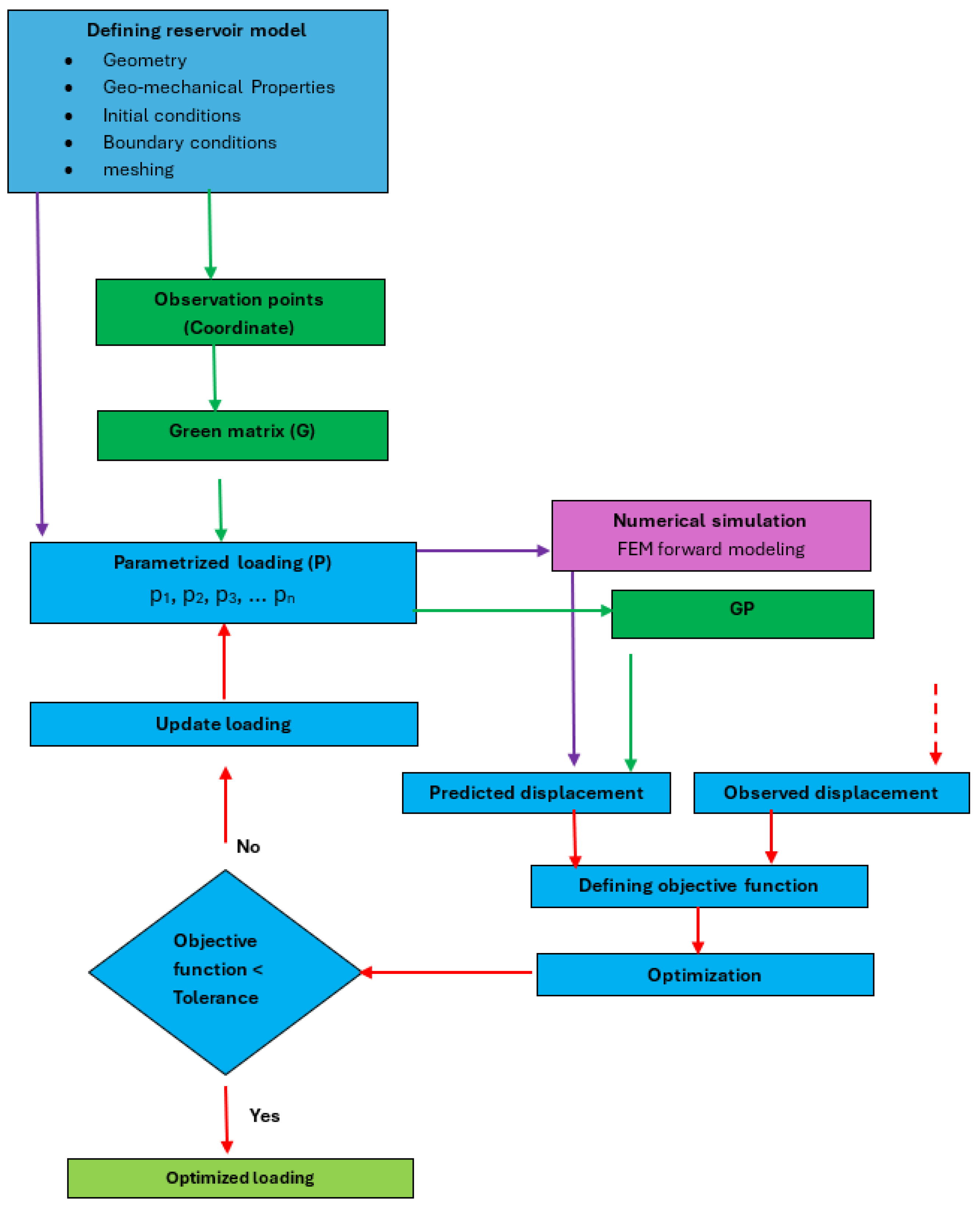
The forward model was constructed numerically by building the discrete Green matrix, which encapsulates the influence of the model’s properties and geometry on the displacement field. By precomputing Green’s matrix, we can rapidly evaluate the displacement at any point in response to any arbitrary pressure distribution. This method streamlines the inversion process, reducing computational costs and improving efficiency. Applying the conventional numerical forward model is computationally expensive as it requires re-running the model in each iteration of the inversion process. Figure 1 illustrates the workflow of this approach, highlighting the differences between the conventional numerical model and the discrete Green’s matrix method. Similar steps in both approaches are shown in blue, while steps unique to the discrete Green’s matrix method are highlighted in green, and those unique to the conventional forward model are highlighted in purple. This color coding clarifies the distinct processes and emphasizes the efficiency and computational advantages offered by the discrete Green’s matrix approach over the conventional method. The initial step involves constructing a detailed model of the geological reservoir using the FEM. This model incorporates the complex geometries and boundary conditions of the reservoir, accurately representing its physical and mechanical properties as well as those of the surrounding media. To construct Green’s matrix for a reservoir, it is necessary to determine the influence of each reservoir element on each observation point. By applying a unit pressure to each reservoir element while maintaining zero pore pressure in all other elements and subsequently solving the resulting displacement field using the FEM, the displacement data at each observation point can be estimated. This process is iteratively performed for all n elements, capturing the influence of each element on the displacement field and constructing a comprehensive Green matrix. Therefore, each component of the Green matrix represents the displacement at a specific observation point due to a unit pressure applied at a particular reservoir element. To automate and accurately build this Green’s matrix, the FEM was integrated with Python scripting, enabling precise and efficient computation of the matrix elements. In this approach, Python scripts are meticulously developed to handle multiple aspects of the FEM setup. This includes scripting the model’s geometry, defining the material properties, and setting up the assembly, boundary conditions, initial conditions, and the steps for loading conditions.

Figure 1.
Inversion workflow for imaging reservoir pressure distribution from deformation data.
Once the basic FEM model is scripted, the Python scripting extends to initiating a loop or automated process to run the model for each reservoir element individually. In each iteration of the loop, a unit pressure load is applied to a selected reservoir element while ensuring that all other elements maintain zero pressure. This script is applied as an input in the FEM model to calculate the Green matrix. This automation ensures that the Green’s matrix is conducted systematically and accurately for any scenario.
If G is the discrete Green’s matrix, P is the pressure distribution vector, and d is the displacement vector at the observation points, the relationship can be described as follows:
d = GP
Here, G is an m × n matrix where each element Gij represents the displacement at the i-th observation point due to a unit pressure applied at the j-th reservoir element (Figure 2). The vector P contains the pressure values for the n reservoir elements, and d contains the resultant displacements at the m observation points.
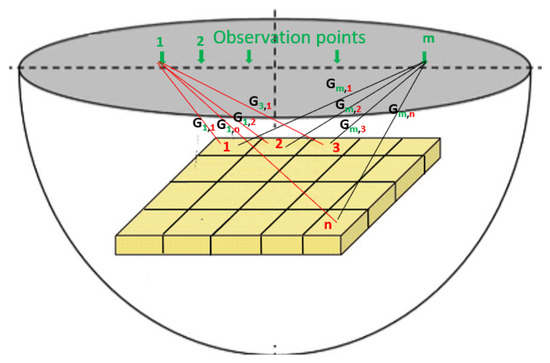
Figure 2.
Schematic of Green matrix construction from observation points and reservoir elements.
With the discrete Green matrix precomputed, the inversion process leverages advanced optimization techniques to estimate the pressure distribution from observed surface displacements. The cost function used in this study is defined as
Here, γ acts as a penalty factor for the smoothness constraint, and L represents the Laplacian operator applied to the pressure change distribution. The cost function combines the displacement error and the regularization term to provide a single measure of fit () and smoothness (LP = d0).
GA was employed as the optimization method to minimize the penalty cost function. GA is particularly suitable for this type of problem because it does not require any a priori information about the pressure distribution, making it ideal for situations where gradient-based methods fall short. Unlike gradient-based methods, which can get stuck in local minima and often require initial guesses or prior knowledge about the pressure distribution, GA explores a wide solution space through mechanisms of selection, crossover, and mutation, allowing for a more comprehensive search for the global optimum. This method allows for efficient and accurate estimation of pressure distributions in complex geological scenarios, making it a powerful tool for handling the ill-posed nature of the problem where the number of observation points is much less than the number of unknown parameters.
3. Results
To validate the proposed inversion approach, we applied it across various scenarios, starting from a simple case that mirrors conditions where an analytical forward model is available to more complex, heterogeneous, multilayer, and irregularly shaped geological models. The first scenario involves estimating the constant reservoir pressure from deformation data, which results from applying a uniform pressure within a cylindrical reservoir in an infinite, isotropic, and homogeneous poroelastic medium. This scenario serves as a benchmark to validate the numerical forward model constructed by the discrete Green’s matrix in the proposed inversion approach and the conventional numerical forward model against the analytical forward model, ensuring that the methodology accurately relates surface deformations to subsurface pressure distributions.
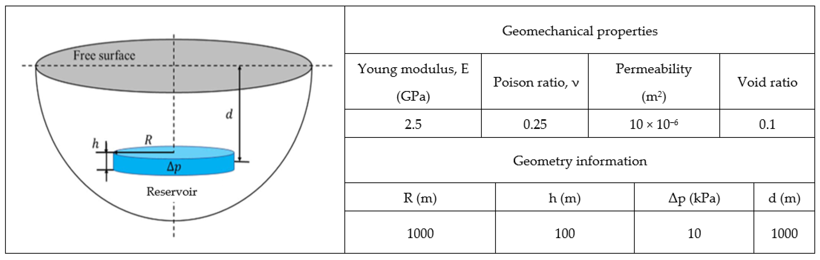
A cylindrical reservoir with a radius of R and a thickness of h, located at a depth of d in an infinite medium (modeled as 10,000 m), and subjected to a constant pore pressure of Δp throughout the whole reservoir, was considered as the first and simplest case. The geo-mechanical properties of the reservoir and the surrounding medium were assumed to be identical. Figure 3 shows the 3D schematic of the model along with the geomechanical properties and dimensions of the reservoir and surrounding porous media.

Figure 3.
Geomechanical properties and geometry of Geertsma analytical model.
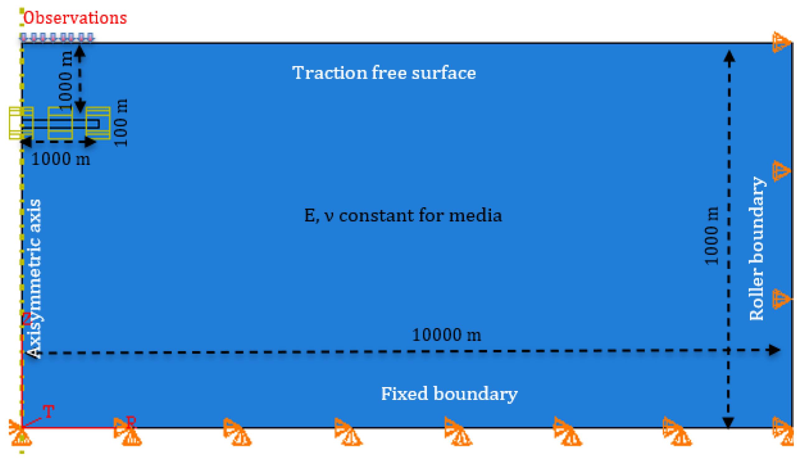
To build the FEM forward model, an axisymmetric 2D approach was selected, which significantly reduces the computational run time compared to a full 3D model. Figure 4 shows the details of the axisymmetric model with boundary conditions specifying a fixed bottom boundary, a traction-free surface, and roller boundaries along the entire outside boundary of the cylinder, except for the bottom and top. The geomechanical properties for all media are listed in Figure 3.
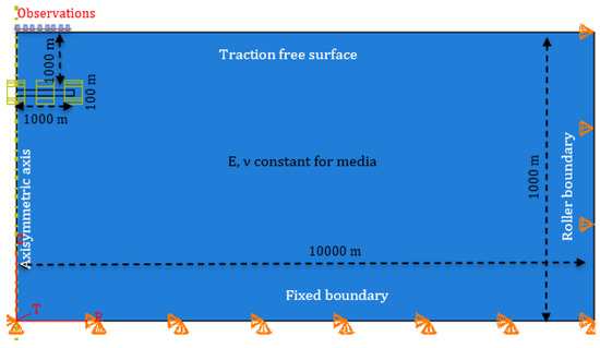
Figure 4.
Geometry and boundary conditions of circular shape reservoir in an infinite media.
The FEM model was tested for result stability with different mesh sizes, and the optimum size was selected for the model. Figure 5 shows the results of vertical displacement at the surface from the center of the model to its boundary with different mesh sizes (coarse, normal, optimized, and fine mesh sizes). As shown in the figure, after reaching the optimized mesh size, further decreasing the mesh size does not affect the results, confirming the independence of numerical results from mesh size. Initially, we tested the coarse mesh; then, we progressively reduced the mesh size to normal, optimized, and fine levels.
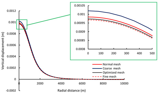
Figure 5.
Numerical result stability test vs. different mesh sizes and selecting the optimum size.
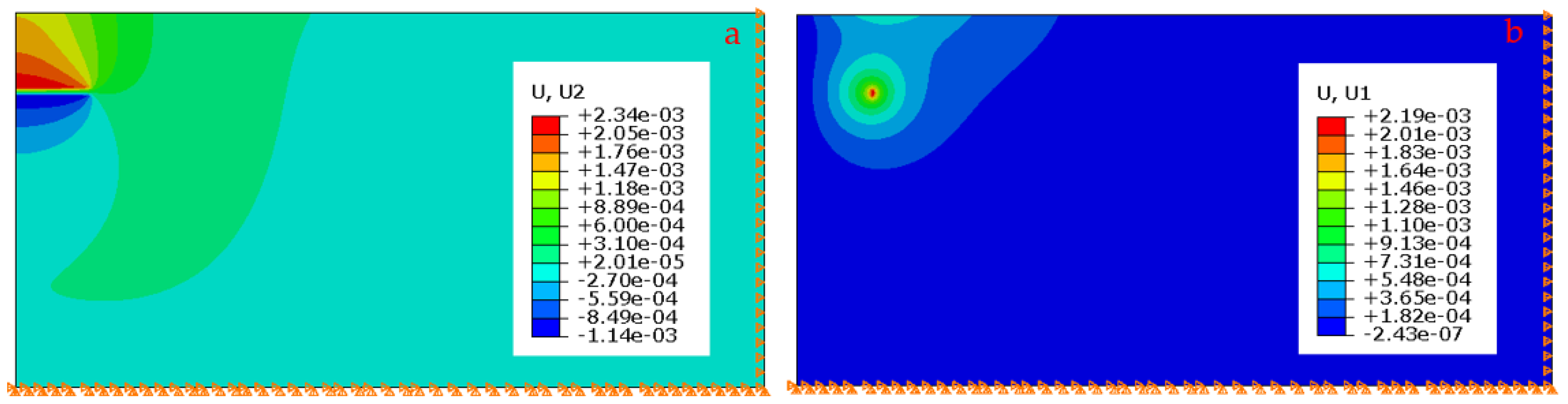
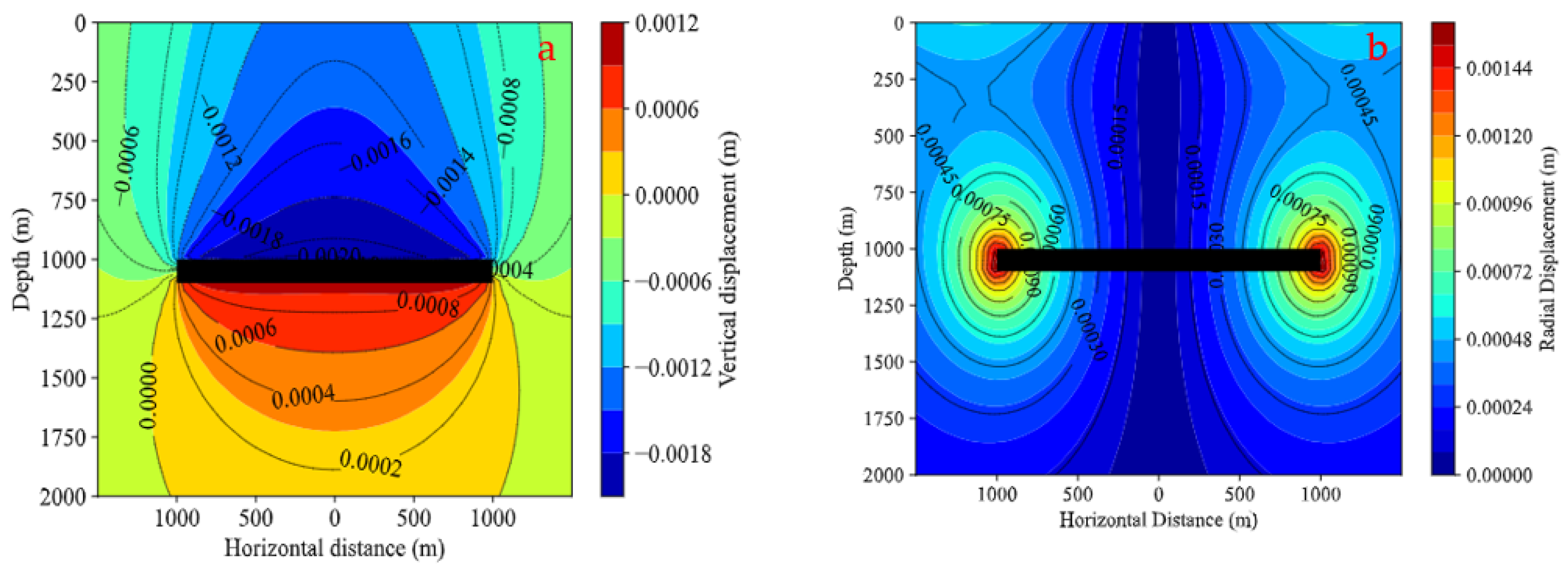
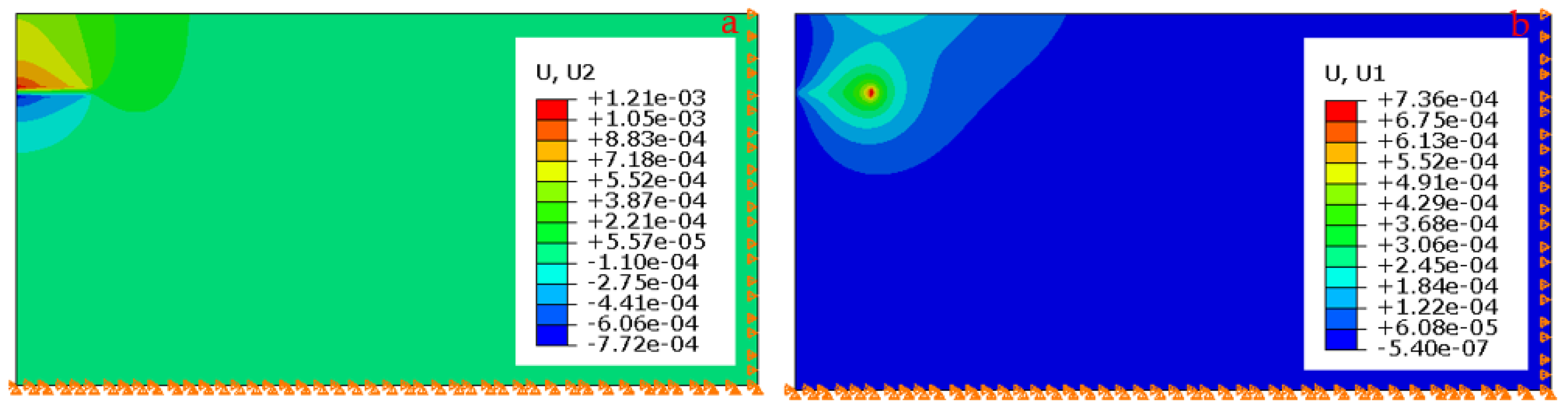
By applying a 10 kPa pore pressure load throughout the cylindrical reservoir, the displacement in the vertical and horizontal directions of all models was compared. Figure 6 shows the resultant vertical (U2) and radial (U1) displacements estimated from the conventional numerical model. Figure 7 depicts the vertical and radial displacements calculated by applying the analytical solution.

Figure 6.
Vertical (a) and radial (b) displacements resulting from a cylindrical constant pressure reservoir (the conventional numerical method).

Figure 7.
Vertical (a) and radial (b) displacements resulting from a cylindrical constant pressure reservoir (analytical method).
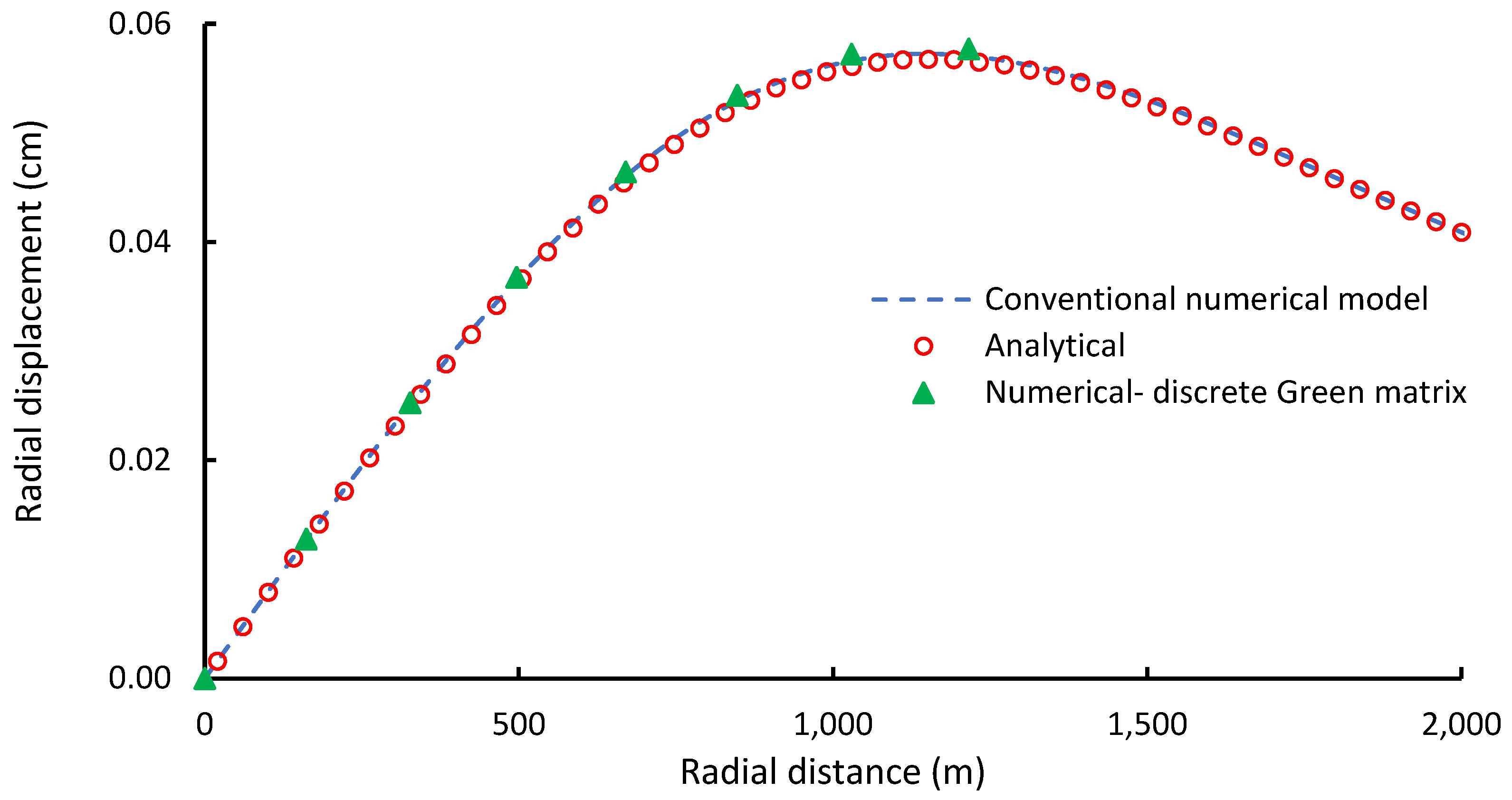
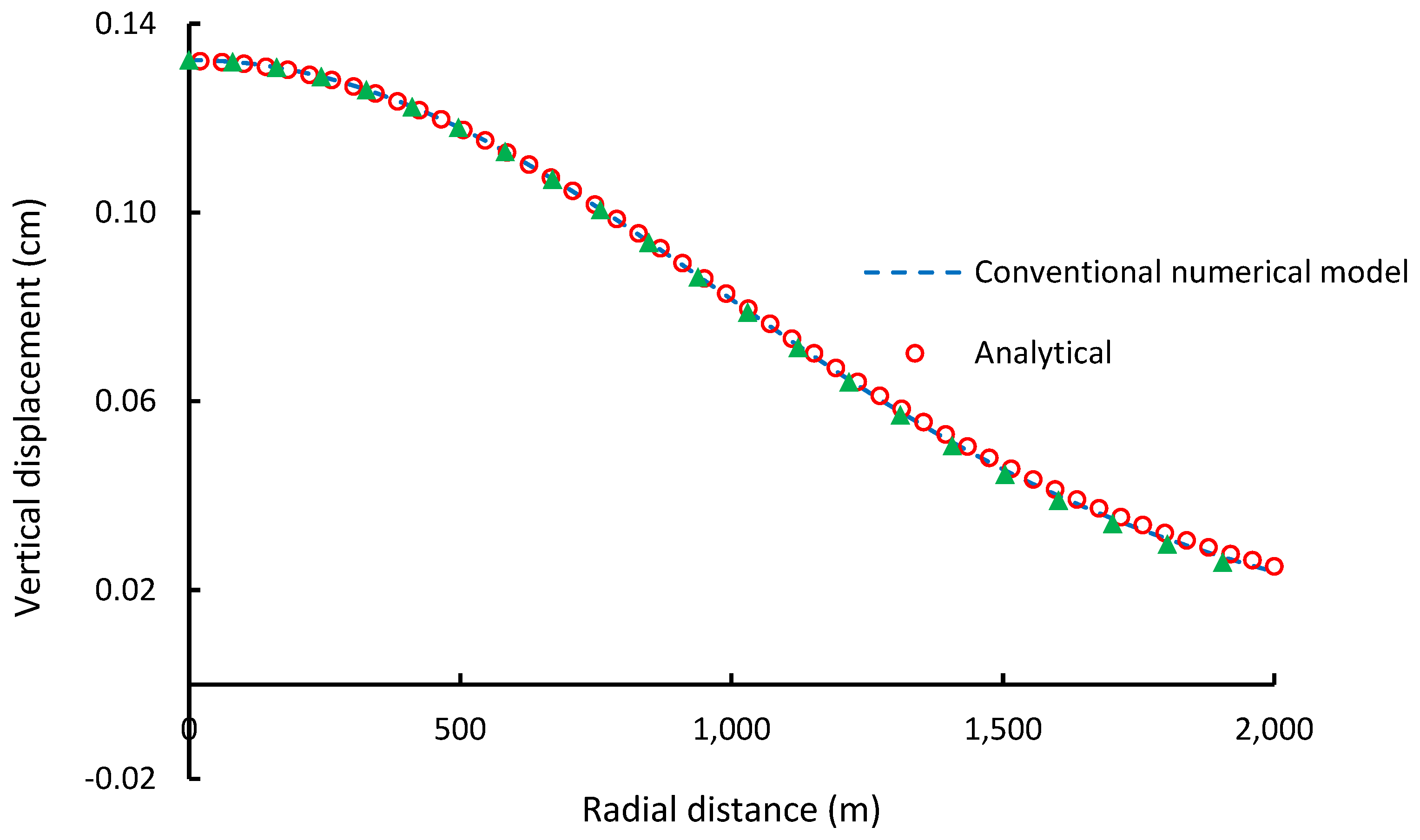
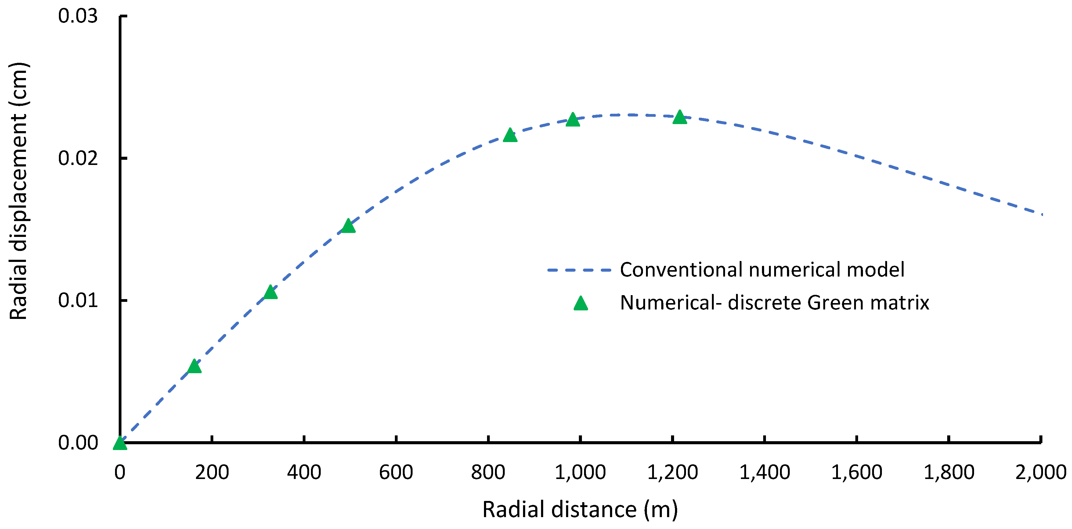
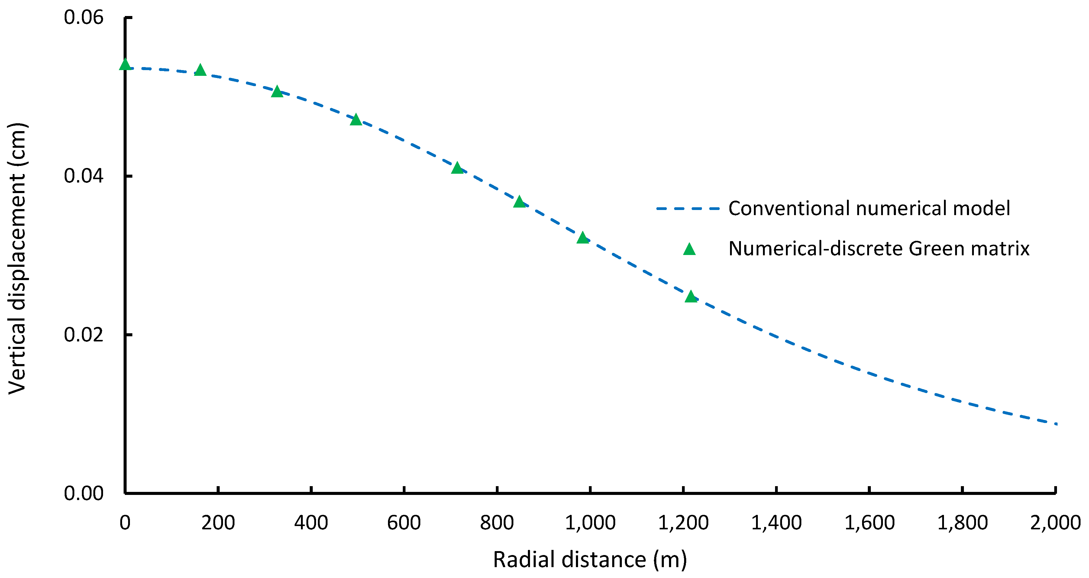
By defining observation points at the model’s surface (the locations of these observation points are shown schematically in Figure 4) and utilizing information related to the number and coordinates of the reservoir elements, we extracted the discrete Green matrix. The matrix multiplication of Green’s matrix with the pore pressure load matrix provided the displacement at the selected observation points. Finally, since the third model provided the deformation at the surface, the resultant displacement at the surface for the first two models was compared with the results of the discrete Green’s matrix approach. Figure 8 and Figure 9 show the displacement results in the radial and vertical directions at the surface for these three models. As shown, the results of the conventional numerical model match the analytical solution completely, verifying the accuracy of the conventional approach. Additionally, the results of the third forward model also match the other models entirely, confirming the reliability of this model for this simple case.
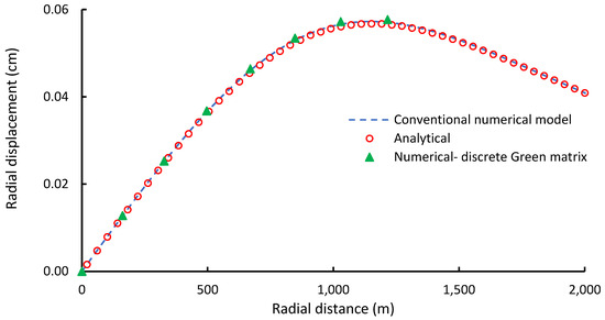
Figure 8.
Comparison of radial displacement at the surface resulting from a cylindrical constant pressure reservoir using different forward models.

Figure 9.
Comparison of vertical displacement at the surface resulting from a cylindrical constant pressure reservoir using different forward models.
Since the analytical solution is available for this scenario, having the deformation at one observation point allows for the exact inversion of this deformation to a constant pressure within the reservoir. Regardless of whether a conventional numerical model or the new forward model is used in the integrated inversion approach, it will promptly yield the exact pressure value.
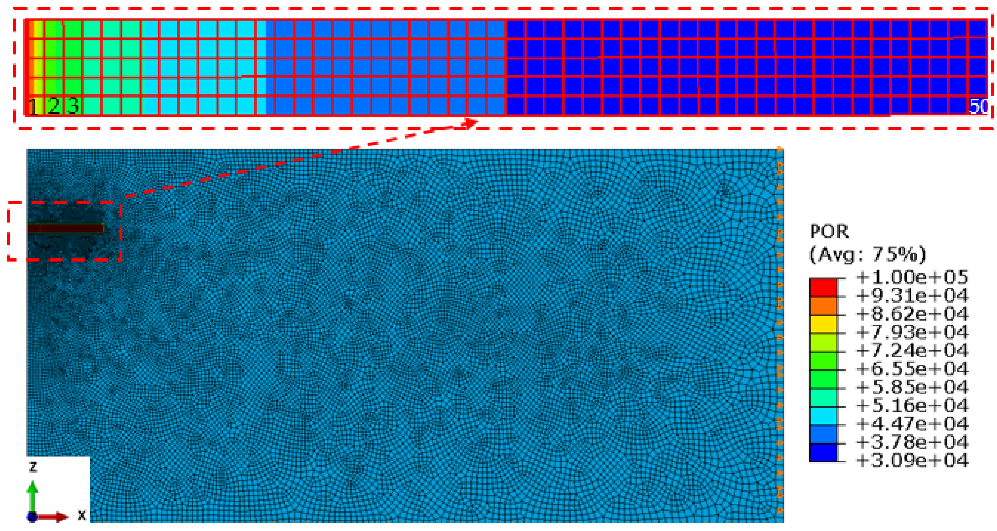
The second scenario is exactly the same as the first scenario except that the pressure was not constant; instead, a distributed pressure throughout the cylindrical reservoir was considered. A logarithmic pressure distribution was used, with a maximum of 10 kPa at the center of the reservoir and logarithmic decline in the radial direction up to the reservoir boundary while the pressure load remained constant in the vertical direction. Regarding the optimized mesh size, each reservoir element was sized at 20 m × 20 m in the 2D profile of the reservoir. With reservoir dimensions of 1000 m × 200 m, this resulted in 250 reservoir elements. Figure 10 shows the arrangement of the reservoir elements and the value of the pore pressure in each element (POR). The reservoir has five rows of elements, and each row contains 50 elements (all elements in the vertical direction have the same pressure, which is clearly indicated by the color code).

Figure 10.
Arrangement of reservoir elements and pressure distribution throughout the cylindrical-shaped reservoir.
Figure 11 shows the resultant vertical (U2) and radial (U1) displacements caused by this logarithmic pore pressure distribution, estimated by the conventional numerical approach.
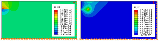
Figure 11.
Vertical (a) and radial (b) displacements resulting from cylindrical variable pressure reservoir (conventional numerical method).
Applying this distributed load and having the discrete Green matrix from the previous scenario, the resultant deformation at the observation points on the surface was estimated. Figure 12 and Figure 13 compare the results of the deformation estimated by the application of a discrete Green matrix with the conventional forward model. Both horizontal and vertical displacements at the surface show a complete match, which confirms the reliability of the discrete Green matrix in estimating the deformation for variable load conditions.
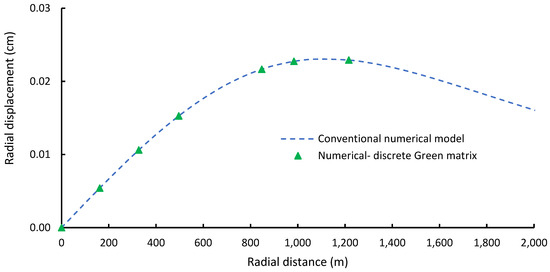
Figure 12.
Comparison of radial displacement at the surface resulting from a cylindrical reservoir (distributed pore pressure) using conventional numerical model and discrete Green matrix.
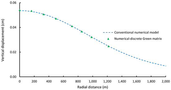
Figure 13.
Comparison of vertical displacement at the surface resulting from a cylindrical reservoir (distributed pore pressure) using conventional numerical model and discrete Green matrix.
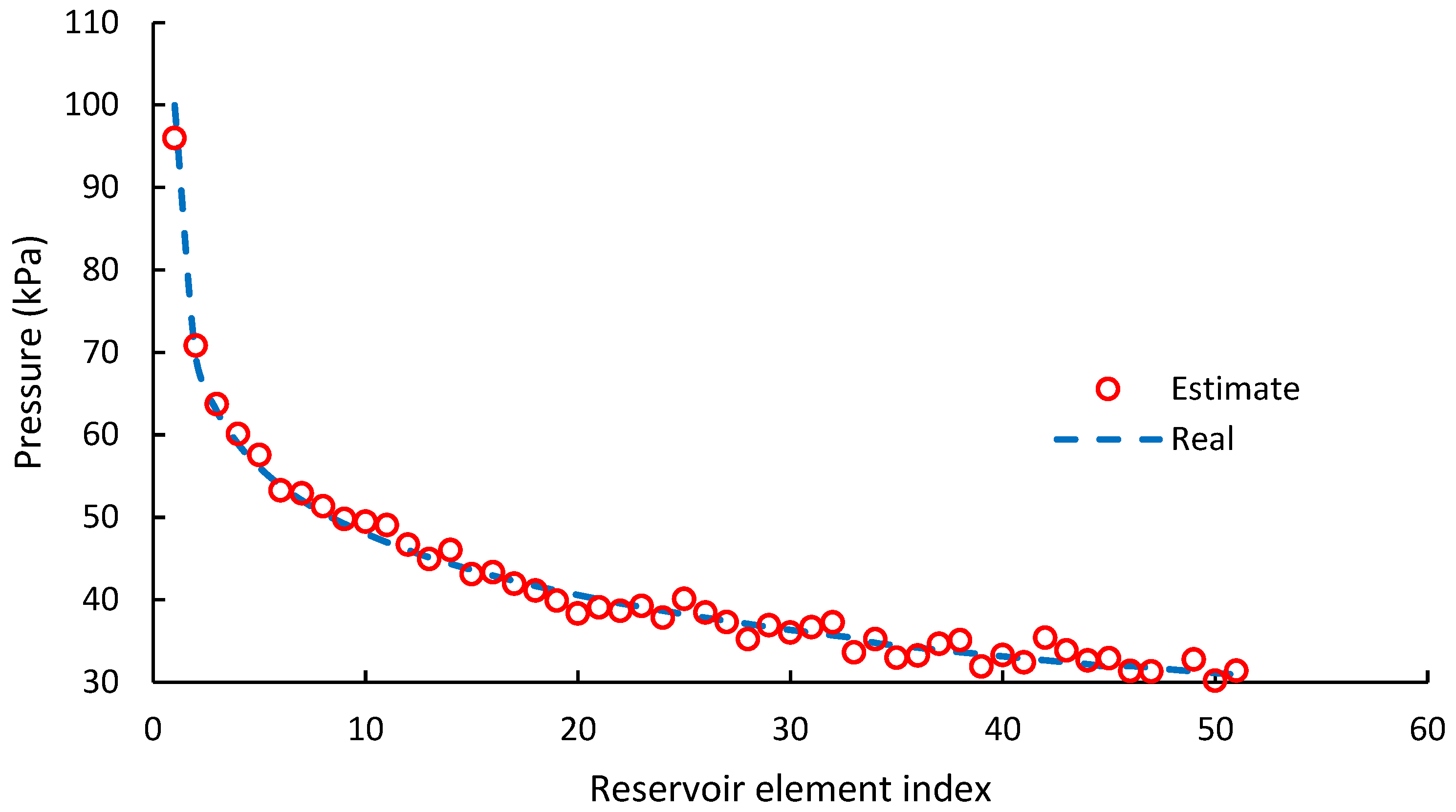
With the first core of the inversion approach (numerical forward model) validated, we performed an inversion using synthetic data. We utilized a limited number of observed data points from the surface (eight deformation data points from the numerical results in Figure 11) to estimate the pressure distribution throughout the reservoir. Given the assumption of zero pressure variation in the vertical direction, the reservoir consists of 250 elements with 50 unknown pressure values. This setup results in an ill-posed problem (50 unknowns and only eight observation points) that can theoretically yield infinite solutions. The optimization component of the integrated inversion model is designed to address this challenge effectively.
Figure 14 shows the result of inversion using the discrete Green matrix to define the forward model and the genetic algorithm as the optimization method. The estimated pressure distribution (50 unknown values, P1 to P50) closely matches the real data, demonstrating the applicability of this integrated approach for distributed pressure loads in the reservoir.
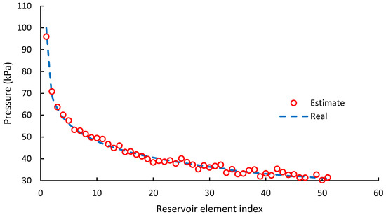
Figure 14.
Comparison of estimated pressure distribution (inversion) with real pressure distribution for cylindrical-shaped reservoir.
In the first and second scenarios, the reservoir and the surrounding layers possessed similar properties, and the reservoir had a simple cylindrical shape with symmetry around the z-axis. While these scenarios provide a simplified context for initial validation, they do not accurately represent the complexities of real-world reservoirs, which often have irregular geometries and varying properties.
We considered a complex scenario to evaluate the reliability of our inversion approach under more realistic conditions. The model consists of multiple layers with different geomechanical properties and varying dip angles in this scenario. The reservoir and surrounding layers lack symmetry, resulting in an entirely irregular system. This setup aims to more accurately reflect the heterogeneous nature of actual geological formations and rigorously test the robustness of our integrated inversion method.
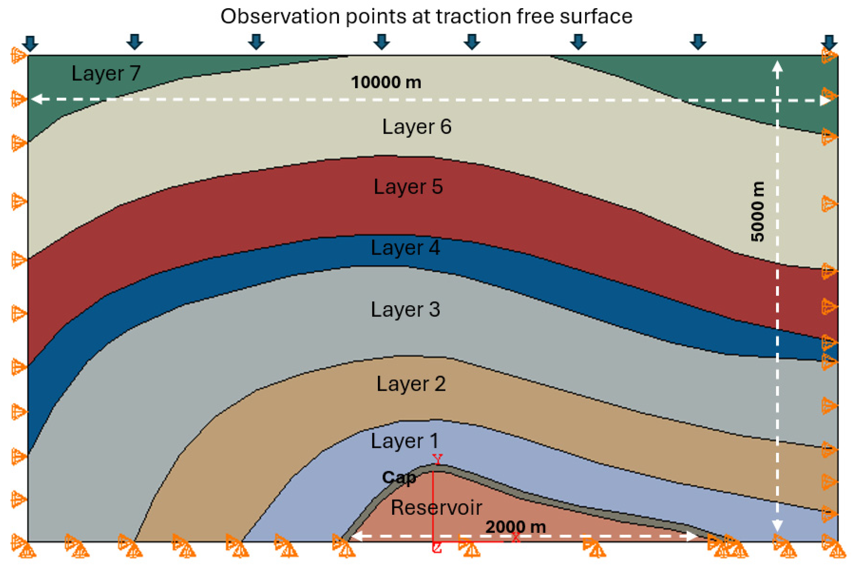
Figure 15 represents the model geometry (the model extends horizontally 10,000 m and has a depth of 5000 m), boundary conditions, and the location of observation points on the surface. The fixed boundary condition was applied at the bottom, traction-free boundary condition was applied at the surface, and roller boundary condition was applied at the right and left sides of the model. The geomechanical properties of all layers (reservoir, cap, and all other layers (seven layers)) are summarized in Table 1.
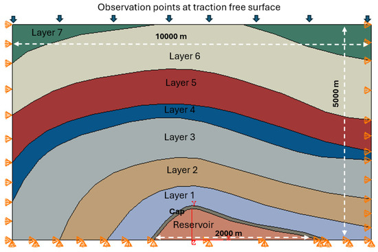
Figure 15.
Schematic of reservoir and overlaying layers in scenario 3.

Table 1.
Geomechanical properties for reservoir and overlaying layers.
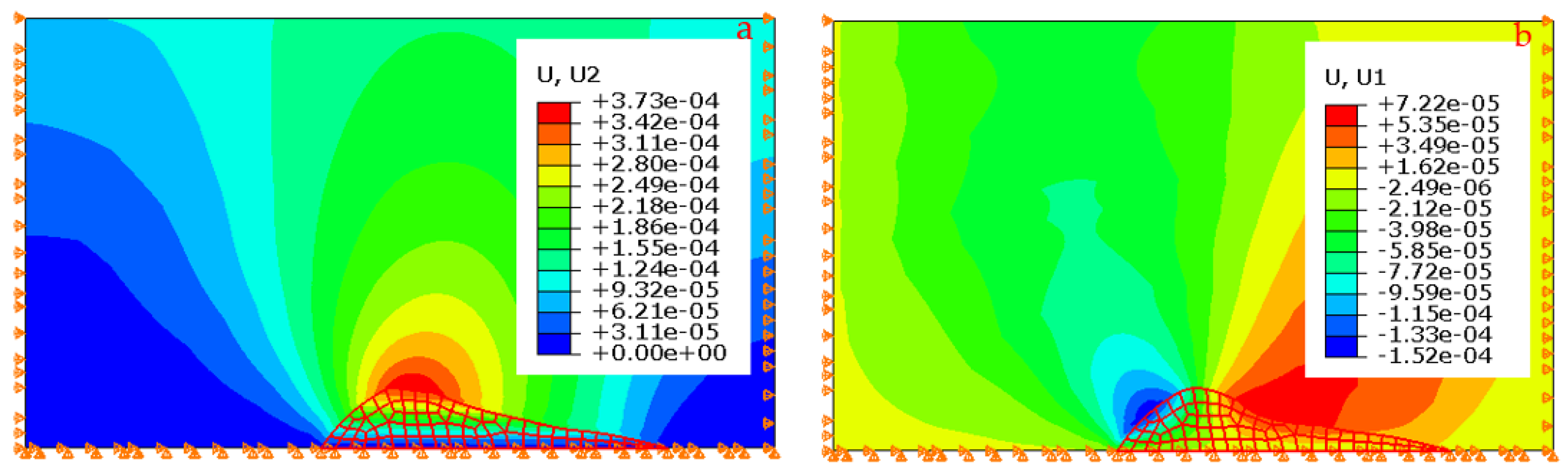
Considering a constant pressure (10 kPa) for all reservoir elements, the resultant deformation in the horizontal (U1) and vertical (U2) directions was estimated by a conventional numerical approach, and the deformation data are represented in Figure 16 (the color code shows the displacement variation, and the reservoir elements are displayed in a red network).
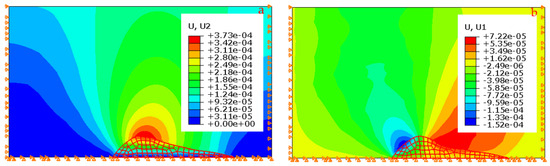
Figure 16.
Vertical (a) and horizontal (b) displacements resulting from constant pressure irregular shape reservoir (conventional numerical method).
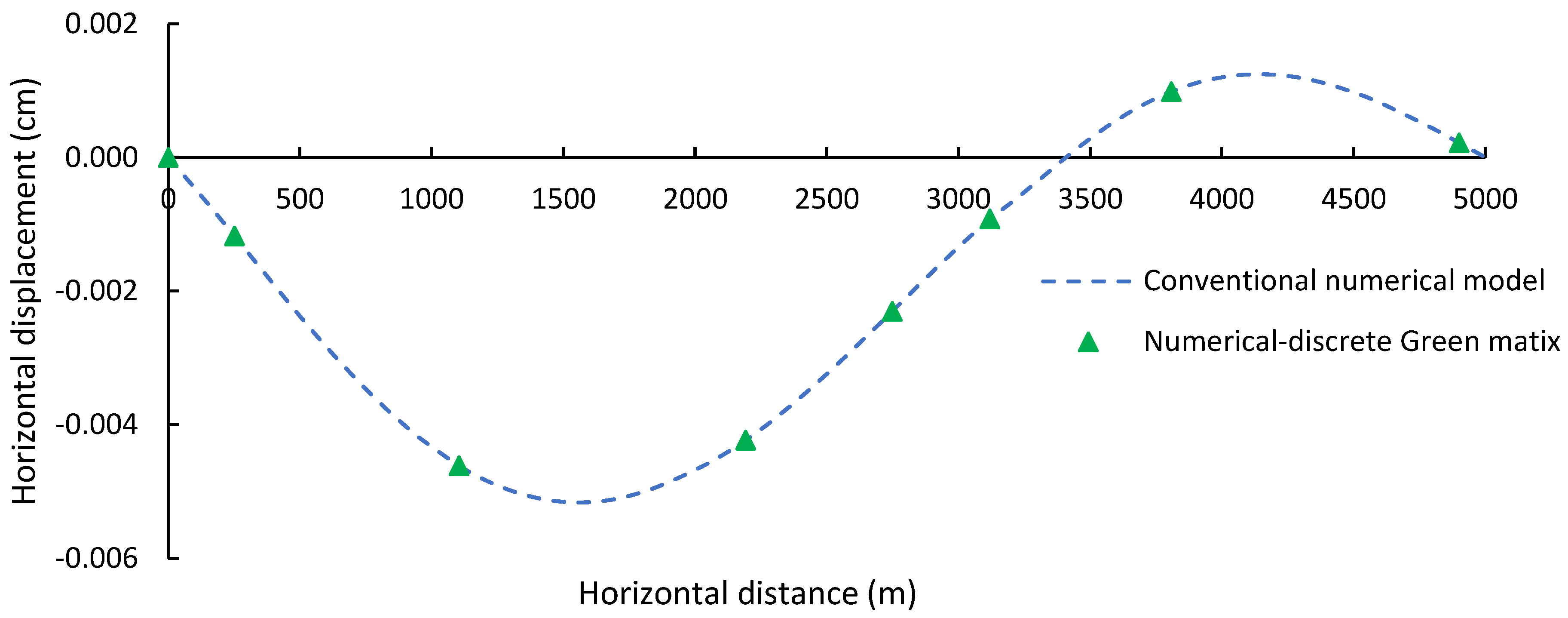
Using the discrete Green matrix for defining the forward model, the same loading conditions as in the conventional approach were applied to estimate the resultant deformation data in both horizontal and vertical directions at the observation points (eight observation points at the surface of the model (Figure 15)). Figure 17 and Figure 18 illustrate a comparison between the results obtained from both forward models, demonstrating a complete match. This confirms the robustness and reliability of the discrete Green matrix, even in complex scenarios with irregular geometries and varying properties.
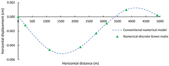
Figure 17.
Comparison of horizontal displacement at surface estimated from conventional forward model and discrete Green matrix.
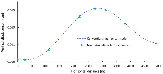
Figure 18.
Comparison of vertical displacement at surface estimated from conventional forward model and discrete Green matrix.
Regardless of the numerical forward model used (conventional or discrete Green matrix), the inversion process is straightforward since there is only one unknown—the constant pressure throughout the reservoir. Even with limited observation data, the pressure can be accurately estimated, resulting in negligible error. This simplicity arises because the constant pressure assumption reduces the complexity of the problem, making it easily solvable despite the limited data points available.
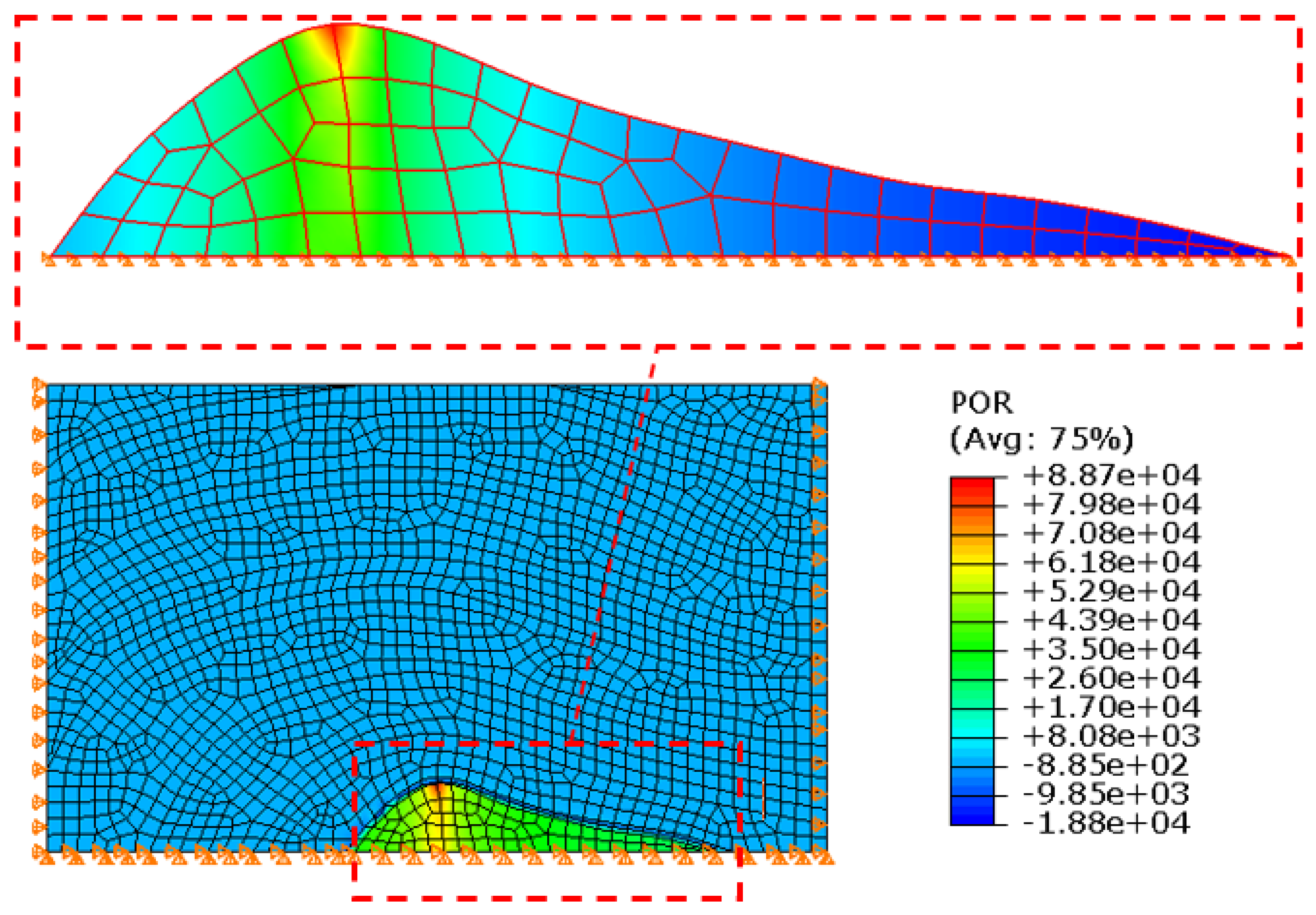
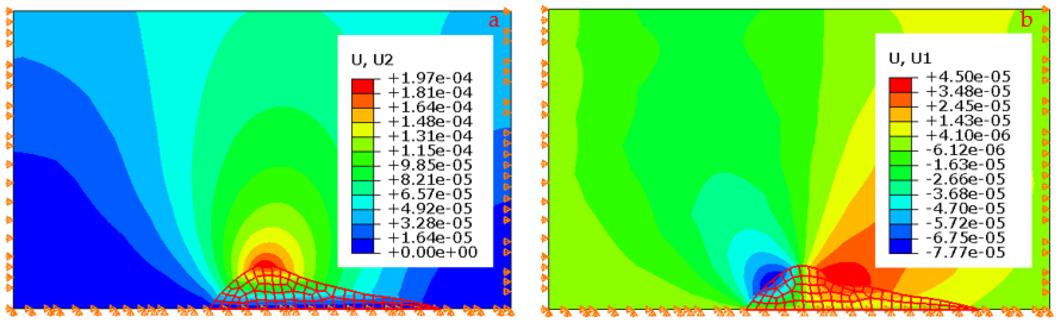
With the numerical forward model validated for an irregular-shaped reservoir, we performed an inversion using a distributed load in this complex geometry for the final scenario. The reservoir consists of 79 elements, each with varying pore pressure values. Figure 19 illustrates the reservoir elements and the applied pore pressure distribution. The maximum pore pressure was applied at the center of the anticline and dissipated toward the reservoir’s boundaries. The color coding in Figure 19 shows the pore pressure distribution (POR) throughout the reservoir. Using the numerical forward model, we estimated the resultant deformation caused by this pore pressure distribution. Figure 20 presents the deformation results in the horizontal (U1) and vertical (U2) directions.
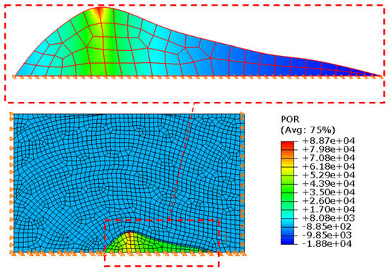
Figure 19.
Arrangement of reservoir elements and pressure distribution throughout the irregular-shaped reservoir.
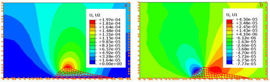
Figure 20.
Vertical (a) and horizontal (b) displacements resulting from distributed pressure in the irregular-shaped reservoir (conventional numerical method).
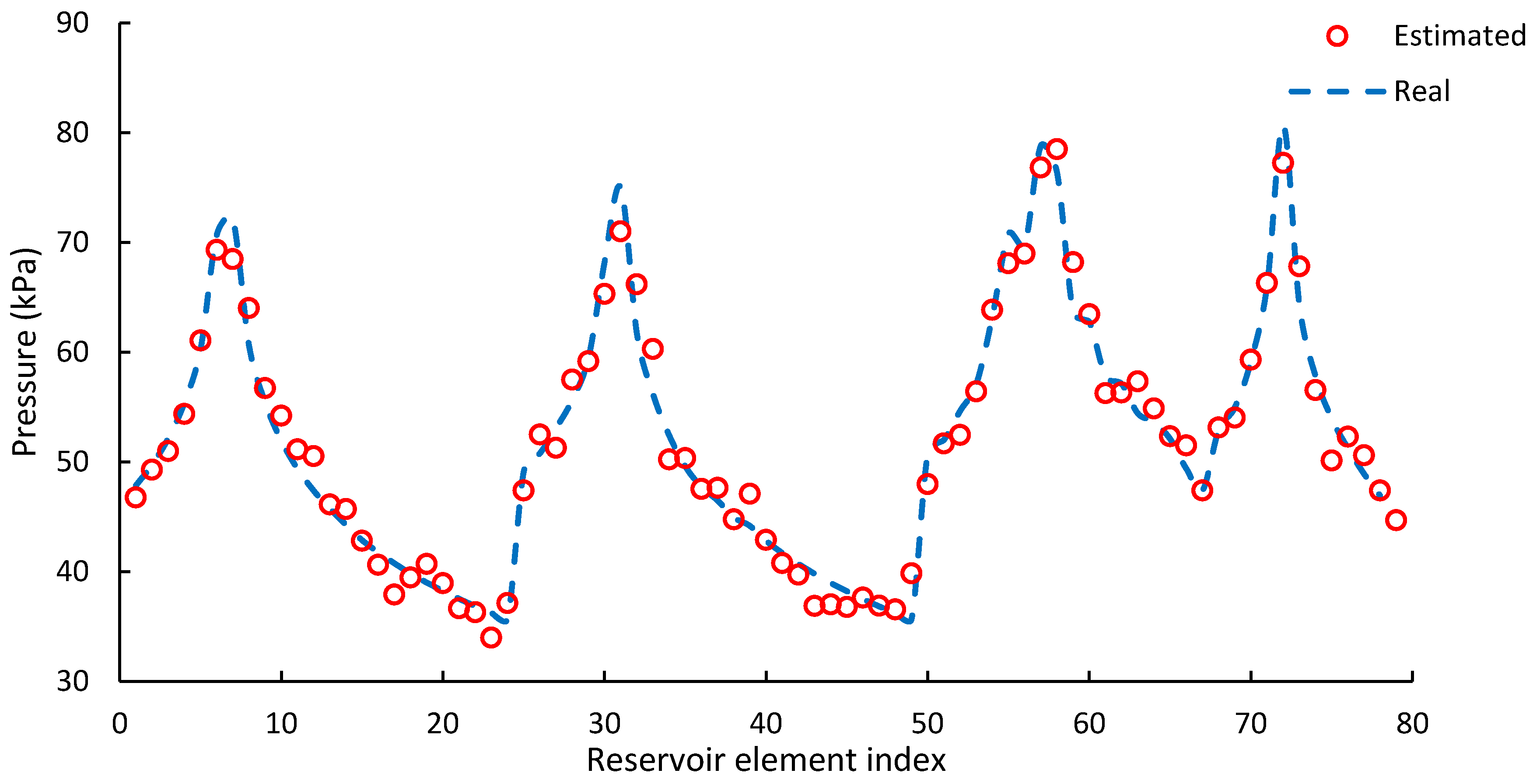
To evaluate the accuracy of the inversion approach, we utilized eight observed deformation points from the synthetic forward model (Figure 20) to estimate the pressure distribution within the reservoir. In this scenario, the model includes 79 unknowns and only eight observation points, resulting in an ill-posed problem. The optimization component of the integrated inversion model is specifically designed to address this challenge. Figure 21 compares the estimated pressure values across all elements with the actual data, demonstrating an acceptable match and confirming the approach’s efficacy.
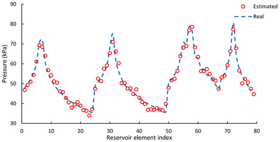
Figure 21.
Comparison of estimated pressure distribution (inversion) with real pressure distribution in irregular-shaped reservoir.
4. Discussion
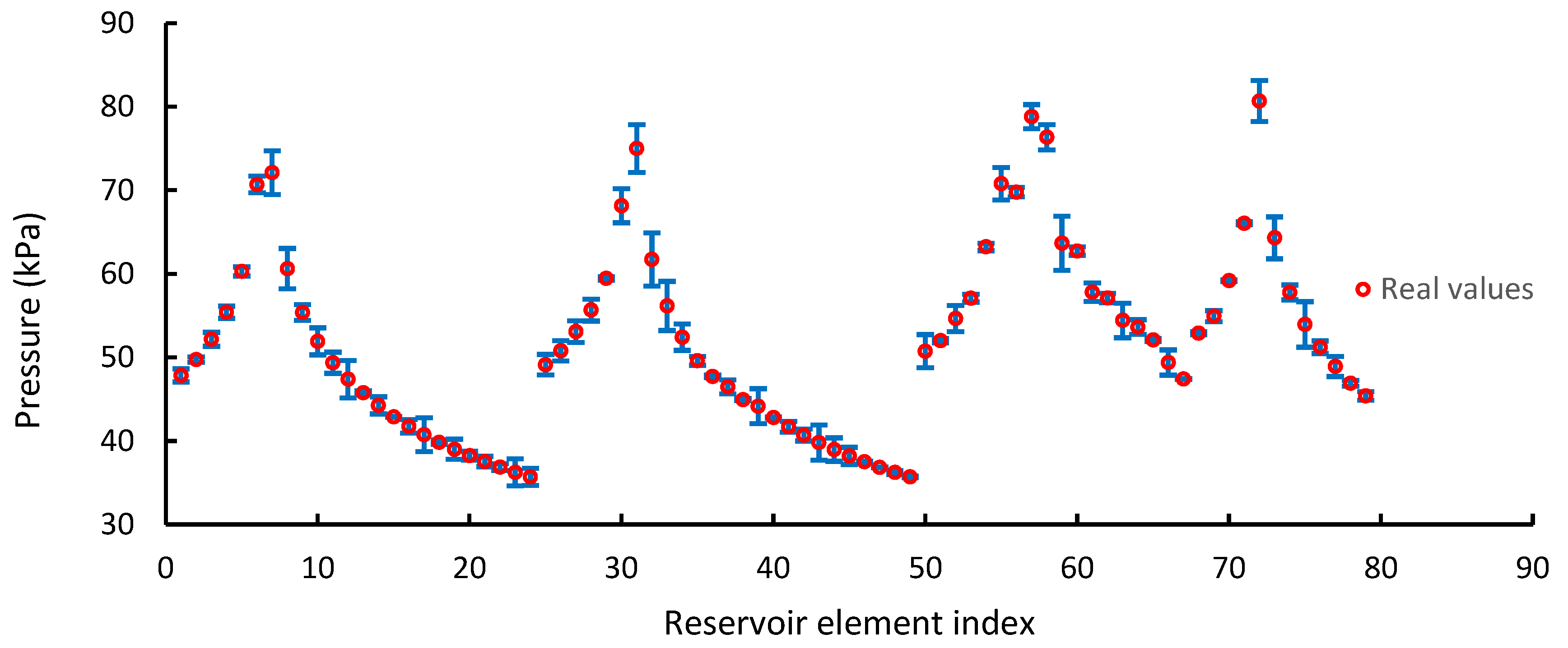
This study introduces an integrated inversion approach that combines an advanced numerical forward model—constructed based on the nucleus of strain concept—with genetic algorithms (GA), a robust optimization tool. This integration is designed to accurately map reservoir pressure from limited surface deformation data. In any optimization endeavor, certain factors, including accuracy, speed, the necessity for reliable initial data, and the adaptability of the model across various scenarios of differing complexities and conditions, are crucial. This section will discuss how our approach excels in meeting these criteria. Reviewing the results from the previous section, we confirmed that our forward model, based on Green’s matrix, aligns perfectly with the conventional numerical forward model across various scenarios, demonstrating its versatility without restrictions in its application. Moreover, the inversion results highlight the model’s precision in estimating pressure distribution, achieving 95% accuracy even in the most complex reservoir cases. Notably, this model operates without prior or initial guesswork, underscoring its robustness in achieving such high precision (95%) without initial data. Figure 22 is dedicated to visualizing the inversion error for the last scenario, allowing for a detailed examination of the discrepancies between the predicted and real values. As the figure illustrates, the maximum error within the elements is approximately 5%, demonstrating the model’s accuracy in predicting pressure using just eight observation points for this complex case.

Figure 22.
Error distribution across reservoir elements for pore pressure prediction.
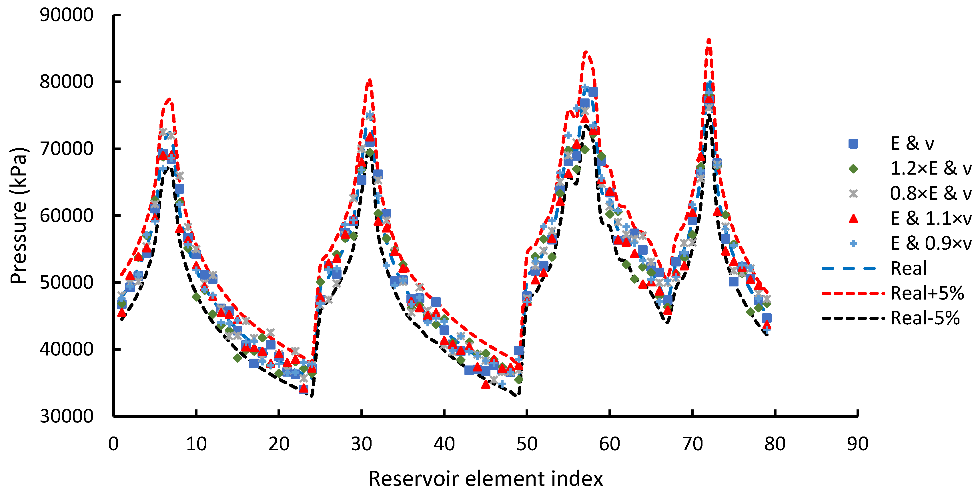
To assess the robustness of our model under various geomechanical conditions, a sensitivity analysis was conducted using varying fundamental properties—Young’s modulus and Poisson’s ratio—across all layers of the geological model. Young’s modulus was adjusted to 20% above and below its base case value, and Poisson’s ratio was varied by ±10%. This analysis aimed to explore these variations’ impact on the accuracy of the model’s pressure predictions. The results of the predicted pressure for all cases were compared against real pressure data depicted in Figure 23. Although the results across these cases varied, the error range remained within 5%. We illustrated the boundaries of ±5% in the figure. As observed, the pressure in all elements of the reservoirs was located between these two boundaries, confirming the reliability of the model and its independence from geomechanical property variations.
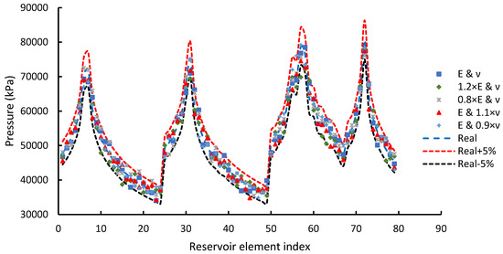
Figure 23.
Sensitivity analysis of inversion approach concerning geomechanical properties.
These results demonstrate that the model is accurate even in complex cases and does not require any prior information, making it suitable for various reservoir scenarios. However, an essential aspect of the inversion model is its efficiency in terms of computational speed. The following question remains: Is this model fast? This aspect is crucial, as the ability to quickly process data and provide results can significantly enhance the model’s usability in practical applications where decision-making speed is often as critical as accuracy.
Implementing a conventional numerical forward model in the optimization loop of inversion can be computationally expensive. Each iteration typically necessitates re-running the FEM forward model to assess the suitability of the proposed pressure distribution. The FEM running requires solving a series of partial differential equations across a discretized domain, which accounts for the reservoir’s geometry, boundary conditions, and material properties.
In contrast, this study uses a numerical forward model based on the discrete Green’s function matrix, which obviates the need to re-run the entire FEM model during each optimization iteration. Green’s function matrix incorporates the geometric and geomechanical properties of the reservoir in advance. Displacement fields are rapidly calculated by simply multiplying this matrix with the pressure distribution array for each iteration. This method significantly decreases the computational time, streamlining the optimization process.
The enhancement in processing speed markedly improves the model’s utility for real-time optimization and decision-making, particularly in complex geological scenarios. For instance, if an optimization process requires approximately 200 iterations—a somewhat optimistic count—and assuming that each iteration of the forward model runs in one minute, which is extremely optimistic for complex models, the total computation would extend to 200 min. Such a duration would render the process impractical for real-time monitoring applications.
However, with the adoption of the discrete Green matrix approach for porous media, the forward model’s runtime is virtually eliminated, replaced by straightforward matrix multiplication.
Our study demonstrates a significant advancement over previous methods by delivering enhanced accuracy and applicability to complex cases, thereby setting a new benchmark in the field. Du and Olson (2001) developed a semi-analytical solution for predicting and mapping subsurface pressure fronts from surface deformation data. Although their model demonstrated excellent precision in estimating pore pressure, it was confined to simple, regularly shaped reservoirs with uniform properties. This limitation restricts its applicability to more complex geological settings [30]. Tang et al. (2022) utilized InSAR data for elastic inversion in West Texas, employing a combination of elastic dislocation and poroelastic reservoir compaction/inflation analytical models. Their approach, while innovative, reported an error range of 10–15% in fault slip and pressure estimation, indicating a need for improved accuracy in more challenging applications [57]. In another notable study, Chaoyang Hu et al. (2021) explored the use of a convolutional neural network (CNN) for geological data inversion. Their advanced image-to-image CNN, trained using a forward evolution method, could predict changes in pore pressure with an accuracy of 83.12%. Despite this advancement, the reliance on extensive training data and significant computational resources highlights a critical limitation, particularly in scenarios requiring rapid decision-making [58].
5. Conclusions
The proposed inversion approach for estimating pressure distribution in geological reservoirs from surface deformation data presents significant advancements. By employing advanced numerical models and genetic algorithms, this technique eliminates the need for a priori information, making it applicable to any reservoir, regardless of its complexity or heterogeneity. The integration of the FEM with Python scripting to construct a discrete Green matrix allows for precise construction of this matrix, which is a core component of the inversion approach. Precomputing the Green matrix eliminates the need for repeated numerical model runs during each optimization iteration, drastically reducing computation time. This makes the approach especially suitable for applications where rapid feedback is essential, such as in real-time monitoring scenarios. The method’s robustness and reliability are demonstrated by testing complex reservoir scenarios, showing less than 5% error in predicted pressure distribution. A critical application of this inversion model is ensuring reservoir integrity throughout the reservoir’s lifecycle. By accurately mapping pressure distributions, the model can detect any anomalies in pressure, which may indicate leakage or other issues. This is particularly crucial during storage operations, where the stored fluids are valuable, or during disposal operations, where leaks could pose significant hazards. The ability to identify these anomalies promptly allows for timely remedial actions, ensuring the safe and efficient operation of the reservoir.
Author Contributions
Conceptualization, M.H.; Methodology, R.A., D.K. and M.H.; Software, R.A.; Validation, A.M.; Formal analysis, D.K. and S.H.; Writing—original draft, R.A.; Writing—review and editing, A.M. and S.H.; Supervision, M.H. All authors have read and agreed to the published version of the manuscript.
Funding
This research received no external funding.
Institutional Review Board Statement
Not applicable.
Informed Consent Statement
Not applicable.
Data Availability Statement
All data are included in the manuscript. More detailed data can be provided to interested researchers upon request.
Acknowledgments
The authors express their gratitude for the support and funding received from the University of Adelaide and CSIRO (Commonwealth Scientific and Industrial Research Organization) throughout the execution of this research. The assistance and resources provided by these institutions have played a crucial role in facilitating the successful completion of this paper.
Conflicts of Interest
The authors declare no conflicts of interest.
Nomenclature
| Symbol | Parameter | Unit |
| e | Void ratio | - |
| F | Body force per unit volume | N/m3 |
| u | Displacement | m |
| α | Biot–Willis coefficient | - |
| λ | First Lame parameter | Pa |
| μ | Second Lame parameter | Pa |
| Young modulus | Pa | |
| Pore pressure | Pa | |
| Volume strain | - | |
| Poisson ratio | - | |
| Stress | Pa | |
| I | Identity matrix | - |
| T | Matrix transpose | - |
| G | Green function/matrix | - |
References
- Sharifi, J. Evaluation of reservoir subsidence due to hydrocarbon production based on seismic data. J. Pet. Explor. Prod. Technol. 2023, 13, 2439–2456. [Google Scholar] [CrossRef]
- Fibbi, G.; Del Soldato, M.; Fanti, R. Review of the Monitoring Applications Involved in the Underground Storage of Natural Gas and CO2. Energies 2023, 16, 12. [Google Scholar] [CrossRef]
- Fibbi, G.; Beni, T.; Fanti, R.; Del Soldato, M. Underground Gas Storage Monitoring Using Free and Open Source InSAR Data: A Case Study from Yela (Spain). Energies 2023, 16, 6392. [Google Scholar] [CrossRef]
- Li, B.Q.; Khoshmanesh, M.; Avouac, J.P. Surface Deformation and Seismicity Induced by Poroelastic Stress at the Raft River Geothermal Field, Idaho, USA. Geophys. Res. Lett. 2021, 48, e2021GL095108. [Google Scholar] [CrossRef]
- Shirzaei, M.; Ellsworth, W.L.; Tiampo, K.F.; González, P.J.; Manga, M. Surface uplift and time-dependent seismic hazard due to fluid injection in eastern Texas. Science 2016, 353, 1416–1419. [Google Scholar] [CrossRef] [PubMed]
- Williams-Stroud, S.; Bauer, R.; Leetaru, H.; Oye, V.; Stanek, F.; Greenberg, S.; Langet, N. Analysis of microseismicity and reactivated fault size to assess the potential for felt events by CO2 injection in the illinois basin. Bull. Seismol. Soc. Am. 2020, 110, 2188–2204. [Google Scholar] [CrossRef]
- Vasco, D.W.; Bissell, R.C.; Bohloli, B.; Daley, T.M.; Ferretti, A.; Foxall, W.; Goertz-Allmann, B.P.; Korneev, V.; Morris, J.P.; Oye, V.; et al. Monitoring and Modeling Caprock Integrity at the In Salah Carbon Dioxide Storage Site, Algeria. Geophysical. Monograph. Ser. 2018, 238, 243–269. [Google Scholar] [CrossRef]
- Cheng, Y.; Liu, W.; Xu, T.; Zhang, Y.; Zhang, X.; Xing, Y.; Feng, B.; Xia, Y. Seismicity induced by geological CO2 storage: A review. Earth Sci. Rev. 2023, 239, 104369. [Google Scholar] [CrossRef]
- Xu, X.Q.; Zhou, H.B. Study on the Influence of Pulse Current Cathodic Protection Parameters of Oil Well Casing. Adv. Mater. Sci. Eng. 2019, 2019, 2847345. [Google Scholar] [CrossRef]
- Han, G.; Liu, Y.; Nawnit, K.; Zhou, Y. Discussion on seepage governing equations for low permeability reservoirs with a threshold pressure gradient. Adv. Geo Energy Res. 2018, 2, 245–259. [Google Scholar] [CrossRef]
- Tipper, J.C. The Study of Geological Objects in Three Dimensions by the Computerized Reconstruction of Serial Sections. J. Geol. 1976, 84, 476–484. [Google Scholar] [CrossRef]
- Eaton, B.A. The Effect of Overburden Stress on Geopressure Prediction from Well Logs. J. Pet. Technol. 1972, 24, 929–934. [Google Scholar] [CrossRef]
- Fillippone, W.R. Estimation of Formation Parameters and the Prediction of Overpressures from Seismic Data. 1982 SEG Annual Meeting; SEG: Houston, TX, USA, 1982. [Google Scholar] [CrossRef]
- Hu, C.; Zhao, W.; Wang, F.; Ai, C.; Wang, T. A new Siamese CNN model for calculating average reservoir pressure through surface vertical deformation. Geomech. Geophys. Geo Energy Geo Resour. 2022, 8, 189. [Google Scholar] [CrossRef]
- Strandli, C.W.; Mehnert, E.; Benson, S.M. CO2 plume tracking and history matching using multilevel pressure monitoring at the Illinois basin—Decatur project. Energy Procedia 2014, 63, 4473–4484. [Google Scholar] [CrossRef]
- Hosseini, S.A.; Shakiba, M.; Sun, A.; Hovorka, S. In-Zone and Above-Zone Pressure Monitoring Methods for CO2 Geologic Storage. Geophys. Monogr. Ser. 2018, 238, 225–241. [Google Scholar] [CrossRef]
- Peyton, J.; Salamaga, J.; McPhee, A.; Jongejan, A. Horner analysis for negative inflow tests of well barriers. SPE Drill. Complet. 2021, 36, 529–541. [Google Scholar] [CrossRef]
- Chen, Z.; Jeffrey, R.G.; Pan, Z. An inversion for asymmetric hydraulic fracture growth and fracture opening distribution from tilt measurements. Int. J. Rock Mech. Min. Sci. 2023, 170, 105539. [Google Scholar] [CrossRef]
- Okada, Y. Internal deformation due to shear and tensile faults in a half-space. Bull. Seismol. Soc. Am. 1992, 82, 1018–1040. [Google Scholar] [CrossRef]
- Robertson, J.O.; Chilingar, G.V.; Khilyuk, L.F.; Endres, B. The environmental aspects of oil and gas production subsidence. Energy Sources Part A Recovery Util. Environ. Eff. 2012, 34, 756–773. [Google Scholar] [CrossRef]
- Mortazavi, A.; Atapour, H. An experimental study of stress changes induced by reservoir depletion under true triaxial stress loading conditions. J. Pet. Sci. Eng. 2018, 171, 1366–1377. [Google Scholar] [CrossRef]
- Ma, X.; Zoback, M.D. Laboratory experiments simulating poroelastic stress changes associated with depletion and injection in low-porosity sedimentary rocks. J. Geophys. Res. Solid Earth 2017, 122, 2478–2503. [Google Scholar] [CrossRef]
- Altmann, J.B.; Müller, B.I.R.; Müller, T.M.; Heidbach, O.; Tingay, M.R.P.; Weißhardt, A. Pore pressure stress coupling in 3D and consequences for reservoir stress states and fault reactivation. Geothermics 2014, 52, 195–205. [Google Scholar] [CrossRef]
- Ramesh Kumar, K.; Hajibeygi, H. Multiscale simulation of inelastic creep deformation for geological rocks. J. Comput. Phys. 2021, 440, 110439. [Google Scholar] [CrossRef]
- Meng, L.; Fu, X.; Lv, Y.; Li, X.; Cheng, Y.; Li, T.; Jin, Y. Risking fault reactivation induced by gas injection into depleted reservoirs based on the heterogeneity of geomechanical properties of fault zones. Pet. Geosci. 2017, 23, 29–38. [Google Scholar] [CrossRef]
- Zhang, G.; Zhu, S.; Zeng, D.; Jia, Y.; Mi, L.; Yang, X.; Zhang, J. Sealing capacity evaluation of underground gas storage under intricate geological conditions. Energy Geosci. 2024, 5, 100292. [Google Scholar] [CrossRef]
- Dusseault, M.B.; Rothenburg, L. Analysis of deformation measurements for reservoir management. Oil Gas Sci. Technol. 2002, 57, 539–554. [Google Scholar] [CrossRef]
- Vasco, D.W.; Karasaki, K.; Myer, L. Monitoring of Fluid Injection and Soil Consolidation Using Surface Tilt Measurements. J. Geotech. Geoenviron. Eng. 1998, 124, 29–37. [Google Scholar] [CrossRef]
- Fokker, P.A. Subsidence Prediction and Inversion of Subsidence Data. In Proceedings of the SPE/ISRM Rock Mechanics in Petroleum Engineering Conference, Irving, TX, USA, 20–23 October 2002. [Google Scholar] [CrossRef]
- Du, J.; Olson, J.E. A poroelastic reservoir model for predicting subsidence and mapping subsurface pressure fronts. J. Pet. Sci. Eng. 2001, 30, 181–197. [Google Scholar] [CrossRef]
- Olson, J.E.; Du, Y.; Du, J. Tiltmeter data inversion with continuous, non-uniform opening distributions: A new method for detecting hydraulic fracture geometry. Int. J. Rock Mech. Min. Sci. 1997, 34, 236.e1–236.e10. [Google Scholar] [CrossRef]
- Fjaer, E.; Holt, R.M.; Horsrud, P.; Raaen, A.M.; Risnes, R. Petroleum related rock mechanics. Pet. Relat. Rock Mech. 1992, 9, 352. [Google Scholar] [CrossRef]
- Lubarda, V.A.; Lubarda, M.V. On the Kelvin, Boussinesq, and Mindlin problems. Acta Mech. 2020, 231, 155–178. [Google Scholar] [CrossRef]
- Mindlin, R.D. Force at a point in the interior of a semi-infinite solid. J. Appl. Phys. 1936, 7, 195–202. [Google Scholar] [CrossRef]
- Mindlin, R.D.; Cheng, D.H. Nuclei of strain in the semi-infinite solid. J. Appl. Phys. 1950, 21, 926–930. [Google Scholar] [CrossRef]
- Geertsma, J. Land Subsidence above Compacting Oil and Gas Reservoirs. J. Pet. Technol. 1973, 25, 734–744. [Google Scholar] [CrossRef]
- Geertsma, J. Problems of rock mechanics in petroleum production engineering. In Proceedings of the 1st ISRM Congress, Lisbon, Portugal, 25 September–1 October 1966. [Google Scholar]
- Segall, P. Induced stresses due to fluid extraction from axisymmetric reservoirs. Pure Appl. Geophys. 1992, 139, 535–560. [Google Scholar] [CrossRef]
- Kosloff, D.; Scott, R.F.; Scranton, J. Finite element simulation of Wilmington oil field subsidence: I. Linear modelling. Tectonophysics 1980, 65, 339–368. [Google Scholar] [CrossRef]
- Baranova, V.; Mustaqeem, A.; Bell, S. A model for induced seismicity caused by hydrocarbon production in the Western Canada Sedimentary Basin. Can. J. Earth. Sci. 1999, 36, 47–64. [Google Scholar] [CrossRef]
- Fredrich, J.T.; Arguello, J.G.; Deitrick, G.L.; De Rouffignac, E.P. Geomechanical modeling of reservoir compaction, surface subsidence, and casing damage at the Belridge diatomite field. SPE Reserv. Eval. Eng. 2000, 3, 348–359. [Google Scholar] [CrossRef]
- Settari, A.; Walters, D.A. Advances in coupled geomechanical and reservoir modeling with applications to reservoir compaction. Soc. Pet. Eng. 2001, 6, 334–342. [Google Scholar] [CrossRef]
- Van Thienen-Visser, K.; Fokker, P.A. The future of subsidence modelling: Compaction and subsidence due to gas depletion of the Groningen gas field in the Netherlands. Neth. J. Geosci. 2017, 96, s105–s116. [Google Scholar] [CrossRef]
- Marketos, G.; Govers, R.; Spiers, C.J. Ground motions induced by a producing hydrocarbon reservoir that is overlain by a viscoelastic rocksalt layer: A numerical model. Geophys. J. Int. 2015, 203, 228–242. [Google Scholar] [CrossRef]
- Lewis, R.W.; Sukirman, Y. Finite element modelling for simulating the surface subsidence above a compacting hydrocarbon reservoir. Int. J. Numer. Anal. Methods Geomech. 1994, 18, 619–639. [Google Scholar] [CrossRef]
- Deng, F.; Dixon, T.H.; Xie, S. Surface Deformation and Induced Seismicity Due to Fluid Injection and Oil and Gas Extraction in Western Texas. J. Geophys. Res. Solid Earth 2020, 125, e2019JB018962. [Google Scholar] [CrossRef]
- Chin, L.Y.; Nagel, N.B. Modeling of Subsidence and Reservoir Compaction under Waterflood Operations. Int. J. Geomech. 2004, 4, 28–34. [Google Scholar] [CrossRef]
- Chan, A.W.; Zoback, M.D. The role of hydrocarbon production on land subsidence and fault reactivation in the Louisiana coastal zone. J. Coast. Res. 2007, 23, 771–786. [Google Scholar] [CrossRef]
- Okada, Y. Surface deformation due to shear and tensile faults in a half-space Okada. Int. J. Rock Mech. Min. Sci. Geomech. Abstr. 1985, 75, 1135–1154. [Google Scholar]
- Lee, H.P.; Staniewicz, S.; Chen, J.; Hennings, P.; Olson, J.E. Subsurface deformation monitoring with InSAR and elastic inversion modeling in west Texas. Geoenergy Sci. Eng. 2023, 231, 212299. [Google Scholar] [CrossRef]
- Vasco, D.W.; Rucci, A.; Ferretti, A.; Novali, F.; Bissell, R.C.; Ringrose, P.S.; Mathieson, A.S.; Wright, I.W. Satellite-based measurements of surface deformation reveal fluid flow associated with the geological storage of carbon dioxide. Geophys. Res. Lett. 2010, 37, L03303. [Google Scholar] [CrossRef]
- Vasco, D.W.; Ferretti, A. On the use of quasi-static deformation to understand reservoir fluid flow. Geophysics 2005, 70, O13–O27. [Google Scholar] [CrossRef]
- Smith, J.D.; Avouac, J.P.; White, R.S.; Copley, A.; Gualandi, A.; Bourne, S. Reconciling the Long-Term Relationship Between Reservoir Pore Pressure Depletion and Compaction in the Groningen Region. J. Geophys. Res. Solid Earth 2019, 124, 6165–6178. [Google Scholar] [CrossRef]
- Du, J.; Brissenden, S.J.; McGillivray, P.R.; Bourne, S.; Hofstra, P.; Davis, E.J.; Roadarmel, W.H.; Wolhart, S.L.; Marsic, S.; Gusek, R.W.; et al. Mapping reservoir volume changes during cyclic steam stimulation using tiltmeter-based surface-deformation measurements. SPE Reserv. Eval. Eng. 2008, 11, 63–72. [Google Scholar] [CrossRef]
- Kabirzadeh, H.; Kim, J.W.; Sideris, M.G.; Vatankhah, S.; Kwon, Y.K. Coupled inverse modelling of tight CO2 reservoirs using gravity and ground deformation data. Geophys. J. Int. 2019, 216, 274–286. [Google Scholar] [CrossRef]
- Vasco, D.W.; Karasaki, K.; Doughty, C. Using surface deformation to image reservoir dynamics. Geophysics 2000, 65, 132–147. [Google Scholar] [CrossRef]
- Tang, H.; Fu, P.; Jo, H.; Jiang, S.; Sherman, C.S.; Hamon, F.; Azzolina, N.A.; Morris, J.P. Deep learning-accelerated 3D carbon storage reservoir pressure forecasting based on data assimilation using surface displacement from InSAR. Int. J. Greenh. Gas Control. 2022, 120, 103765. [Google Scholar] [CrossRef]
- Hu, C.; Wang, F.; Ai, C. Calculation of Average Reservoir Pore Pressure Based on Surface Displacement Using Image-To-Image Convolutional Neural Network Model. Front. Earth Sci. 2021, 9, 712681. [Google Scholar] [CrossRef]
- Rudnicki, J.W. Fluid mass sources and point forces in linear elastic diffusive solids. Mech. Mater. 1986, 5, 383–393. [Google Scholar] [CrossRef]
- Wang, H.F. Theory of Linear Poroelasticity with Applications to Geomechanics and Hydrogeology; Princeton University Press: Princeton, NJ, USA, 2001. [Google Scholar] [CrossRef]
- Parker, R.L. Geophysical inverse theory. Geophysical Inverse Theory. Phys. Today 1994, 48, 92–94. [Google Scholar] [CrossRef]


Disclaimer/Publisher’s Note: The statements, opinions and data contained in all publications are solely those of the individual author(s) and contributor(s) and not of MDPI and/or the editor(s). MDPI and/or the editor(s) disclaim responsibility for any injury to people or property resulting from any ideas, methods, instructions or products referred to in the content. |
© 2024 by the authors. Licensee MDPI, Basel, Switzerland. This article is an open access article distributed under the terms and conditions of the Creative Commons Attribution (CC BY) license (https://creativecommons.org/licenses/by/4.0/).