Article

Skillful Seasonal Prediction of Global Onshore Wind Resources in SIDRI-ESS V1.0

1
Shanghai Investigation, Design and Research Institute Co., Ltd., Shanghai 200434, China
2
Key Laboratory of Polar Atmosphere-Ocean-Ice System for Weather and Climate of the MOE, Department of Atmospheric and Oceanic Science and Institute of Atmospheric Science, Fudan University, Shanghai 200438, China
3
Key Laboratory for Polar Science of the MNR, Polar Research Institute of China, Shanghai 200136, China
*
Author to whom correspondence should be addressed.
Sustainability 2024, 16(17), 7721; https://doi.org/10.3390/su16177721
Submission received: 12 July 2024 / Revised: 18 August 2024 / Accepted: 29 August 2024 / Published: 5 September 2024
(This article belongs to the Section Environmental Sustainability and Applications)

Abstract

:
The seasonal variation in wind resources has a great impact on wind energy generation, affecting the maintenance planning, operational strategies, and economic benefits of wind farms. Therefore, effective seasonal prediction of wind resources is crucial for the wind power industry. This study evaluates the seasonal prediction skill for global onshore wind resources using the SIDRI-ESS V1.0 dynamic prediction system. High prediction skill for 10 m wind speed (ws10m) is observed mainly in six regions: southern North America, northern South America, western and eastern Europe, and South and East Asia. These regions already have a substantial wind power industry or possess rich wind resources and will need wind power industry deployment in the future. Prediction skill is the highest at a 1-month lead time for most regions and decays as the lead time increases. The highest skill emerges in East Asia, with a temporal correlation coefficient (TCC) reaching 0.7, and persists with a 1-month to 5-month lead time. However, the highest skill for southern North America is at a 6-month lead time. Additionally, ensemble prediction effectively reduces uncertainty, such that a multi-member ensemble mean always matches or even exceeds the individual ensemble member with the best performance. Ensemble size analysis shows that increasing the number of ensemble members generally enhances the prediction skill, with 24 members being sufficient for most regions and lead times. However, further increasing the ensemble size is essential to improve the prediction skill at a 6-month lead time. Meanwhile, we also indicate that ws10m can be used as a proxy in evaluating seasonal prediction of wind resources over most regions, while direct seasonal prediction of wind power density is more effective for northern South America. The high seasonal prediction skill of SIDRI-ESS V1.0 highlights its potential for providing valuable seasonal climate prediction services to the wind power industry.

1. Introduction

As a clean and renewable form of energy, wind energy is regarded as a key to achieving global energy transformation due to the increasing maturity of wind power technology and its decreasing cost, and it has made important contributions to mitigating global warming [1,2,3]. The energy and electricity industry often requires wind resource predictions at various timescales, which are crucial for providing high penetration of new energy sources and balanced power dispatch, and for ensuring a stable energy supply [4,5,6,7,8,9].
Wind power accounts for a large portion of global power generation. Renewable energy contributed 30.3% of global total electricity generation in 2023. Wind power is the second-largest source of renewable energy, with its generation reaching 2304 TWh, accounting for 7.8% of global electricity [10,11]. As wind power continues to grow, it is becoming an increasingly vital component of future energy systems. Due to the intermittent and fluctuating nature of wind resources, most attention has been focused on short-term forecasts to ensure the smooth operation of wind turbines and dispatch in power grids [12,13,14,15]. The seasonal variation in wind resources often affects wind power generation and thereby impacts energy management, maintenance planning, and economic benefits for wind farms [6,16,17,18,19,20]. In fact, it has been shown that seasonal prediction can effectively assist in the utilization and management of wind resources by estimating future wind farm output one or more seasons in advance, thus supporting wind farm generation planning, load balancing by grid system operators, and electricity market trading. With the development of the wind power industry, there is a growing interest in and demand for seasonal prediction of wind resources [5,6,9,21,22,23,24,25,26,27,28].
Previous studies have shown skillful seasonal prediction of wind resources by statistical or dynamic models. From the perspective of dynamic models, climate system models or earth system models are often powerful tools for seasonal prediction (Table 1). The Copernicus Climate Change Service (C3S) provides seasonal prediction services for the energy industry and policymakers based on several state-of-the-art seasonal prediction systems [29]. For example, Clark et al. [5] have shown that the fifth generation of the global seasonal prediction system (GloSea5) exhibits considerable predictive skill for winter wind speed and surface temperature over the UK at a 1-month lead time. The seasonal prediction skill for wind speed is derived primarily from the predictability of the North Atlantic Oscillation (NAO), which implies that skillful seasonal predictions of winter electricity demand and energy supply can be achieved by seasonal prediction of the NAO. Some studies have also evaluated the seasonal prediction skill for wind speed over China using GloSea5 with a 1-month lead time. High prediction skill is observed in some regions of China that are impacted mainly by the El Niño–Southern Oscillation (ENSO) and 500 hPa geopotential height. However, prediction skill for summer wind speed is lost in GloSea5 [21,23]. Additionally, many studies have also focused on the potential of providing seasonal climate services based on the other seasonal prediction systems in C3S, particularly for wind energy resources over Europe and North America, or even from a global perspective [6,22,26,27]. Recently, Yang et al. [28] revealed skillful seasonal predictions of wind energy over the U.S. Great Plains in the Seamless System for Prediction and EArth System Research (SPEAR) from the Geophysical Fluid Dynamics Laboratory (GFDL), which could help optimize energy production. Some studies have performed seasonal prediction by using deep learning algorithms or constructing statistical models using specific large-scale circulation information, which also demonstrated considerable predictive skill [25,30,31,32].
Although previous studies have focused primarily on analyzing the seasonal predictive skill for specific seasons at a 1-month lead time, one of the main economic benefits of seasonal prediction for the energy and electricity industry lies in long-term predictions that are as accurate as possible. This capability aids the formulation of long-term energy procurement plans and strategies, thereby offering essential support for trading strategies in the power market. The aim of this study is to investigate the seasonal prediction skill for global onshore wind resources during boral summer, with a lead time of up to six months, using a dynamic ensemble seamless prediction system designed by Shanghai Investigation, Design and Research Institute Co., Ltd. (Shanghai, China) (SIDRI-ESS V1.0).
The structure of this paper is outlined as follows. In Section 2, we introduce the data and methods used in this study, including the observational dataset, model and experiment design, and verification methods. The performance of SIDRI-ESS V1.0 in predicting wind resources is evaluated in Section 3, including the simulation of climatology and the seasonal prediction skill for wind resources. A summary is given in Section 4.

2. Data and Methods

2.1. Observation-Based Data

The 6-hourly Final reanalysis dataset (FNL) derived from the National Centers for Environmental Prediction/National Center for Atmospheric Research (NCEP/NCAR) is used in this analysis as a proxy for observations. The FNL product is generated by the Global Data Assimilation System (GDAS), which assimilates observational datasets from various sources, including ground stations, weather balloons, and satellites [33] (http://dss.ucar.edu/datasets/ds083.2/, accessed on 27 March 2023). The FNL has a grid resolution of 1° × 1° and it has been available from 1999 to the present. The variables used in this study include temperature, humidity, geopotential height, sea level pressure, surface pressure, 10 m winds, and zonal and meridional wind. All variables cover a period of 2000–2022, and 10 m winds are used to calculate 10 m wind speed (ws10m) to verify the seasonal prediction skill of global onshore wind resources.

2.2. Model Description

SIDRI-ESS is the first generation of a fully-coupled global climate model, developed by Shanghai Investigation Design and Research Institute Co., Ltd. (Shanghai, China) (SIDRI), consisting of atmosphere, ocean, land, and sea ice models, which exchanges heat and momentum fluxes via a coupler. The atmosphere model in SIDRI-ESS uses a finite-volume dynamic core [34] and achieves discretization on a cubed-sphere grid system [35] with a horizontal resolution of 1° × 1° (~100 km). The ocean component is the Parallel Ocean Program Version 2 with a 1° × 1° resolution grid (POP2, [36]). The land and sea ice models used in SIDRI-ESS are Community Land Model Version 4 (CLM4, [37]) and Los Alamos Sea Ice Model Version 4 (CICE4, [38]), respectively. Based on this model, we develop the first generation of dynamic seamless prediction system SIDRI-ESS V1.0.

2.3. Experiments Design

Hindcast experiments are designed to evaluate the seasonal prediction skill of SIDRI-ESS V1.0. In the current version, we only performed atmospheric assimilation. Other components (ocean, land, and sea ice) were adjusted with the atmospheric components due to interactions within the climate system. To obtain accurate atmospheric initial conditions, the 6-hourly air temperature, specific humidity, geopotential height, surface pressure, sea level pressure, and zonal and meridional winds from the FNL reanalysis data were assimilated using a time-varying nudging method based on the incremental analysis update method [39]. The nudging time step is 6 h and a 3-year spin-up time from 2000 to 2002 was adopted to obtain a steady integration before hindcasts. Twenty-year hindcasts were generated on the penultimate day of each month with 24 ensemble members for the period of 2003–2022. The 24 ensemble members were generated based on a time-lag perturbation, and each ensemble member has 190-day integration (230-day and 250-day integrations for January and December, respectively). Thus, there are 12 × 24 experiments per year, amounting to a total of 5760 runs. In this analysis, we primarily focus on the prediction skill for onshore wind resources during boreal summer (June-July-August, JJA). The prediction for JJA from May is called a 1-month lead in hindcasts.
We also designed a numerical experiment in which the model was freely integrated for 20 years to obtain a stable mean state of the model itself, which can be used to verify the impact of assimilation on reducing the model biases.

2.4. Verified Method

The seasonal predictive skill of the prediction system for wind resources is evaluated by employing the temporal correlation coefficient (TCC) and normalized root mean square error (nRMSE).
The TCC is used to analyze the linear relationship between predictions and corresponding observations in time evolution; a greater TCC value means a better predictive skill. The TCC is defined as follows:
T C C = i = 1 N F i O i i = 1 N F i 2 i = 1 N O i 2
In which F is the prediction result, O is the observation, i denotes time, N is the length of the time period, and the prime is the anomalies with the climatological mean state removed. A two-tailed Student’s t-test is used to test the statistical significance of the TCC.
The nRMSE is designed to measure biases between prediction values and observations on different scales; nRMSE values close to 0 denote a better predictive skill. The nRMSE is defined as follows:
n R M S E = 1 N i = 1 N F i O i 2 1 N i = 1 N O i 2

3. Results

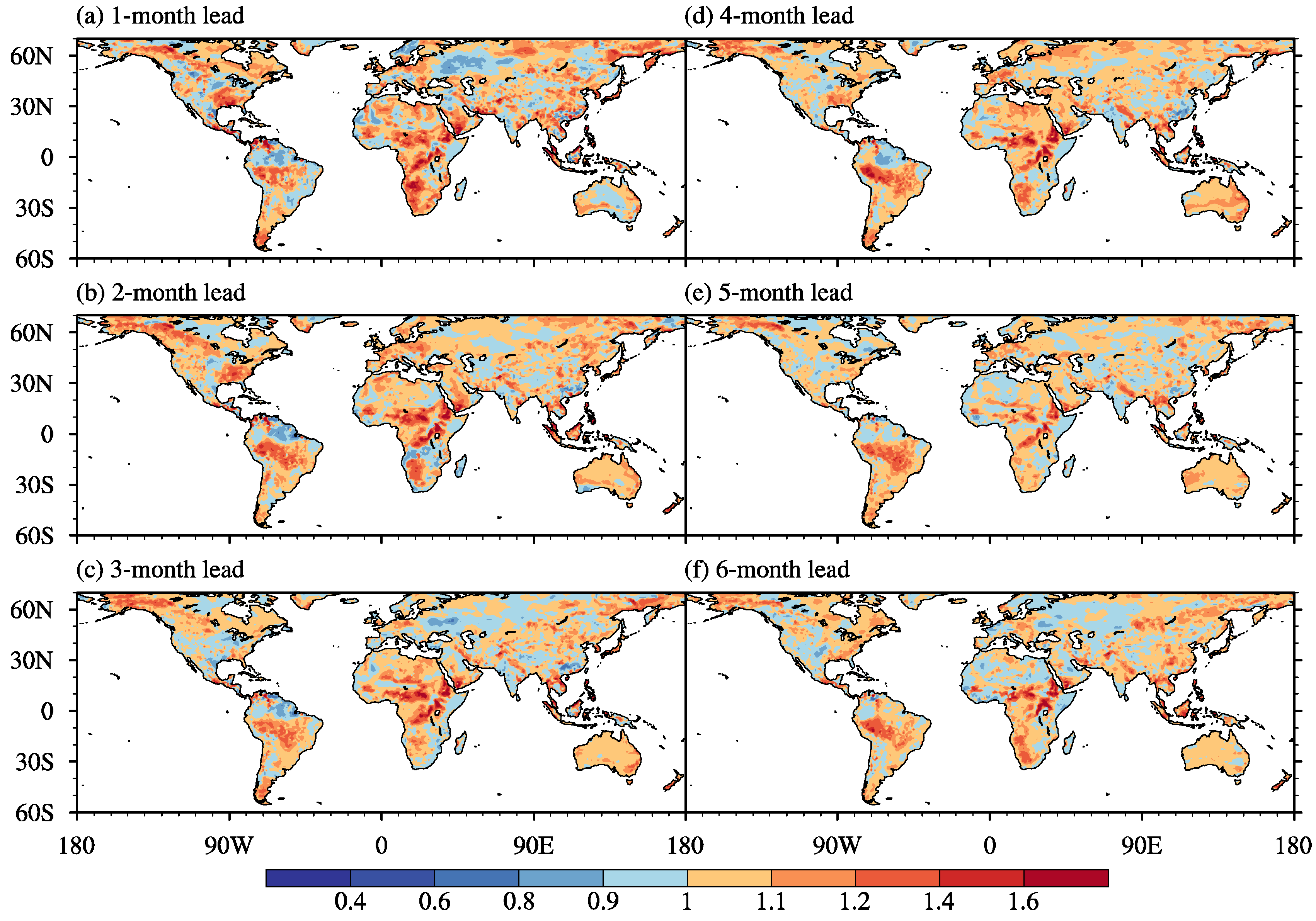
3.1. Simulation of Climatology

Before evaluating the prediction skill for wind resources, it is necessary to verify the model’s ability to simulate the climatology. The effect of assimilation on climatological 10 m wind speed (ws10m) is examined by comparing the results in a free-coupled experiment, nudging experiment, and observations (Figure 1). In observations, abundant onshore wind resources are concentrated mainly in tropical regions (30° S–30° N) during boreal summers, such as southern North America, eastern Brazil, most of Africa, Central Asia, West Asia, South Asia, and southern South America (Figure 1a). The JJA-mean climatological ws10m can reach more than 5 m/s in these regions.
The differences in climatological ws10m between the free-coupled experiment, nudging experiment, and observations are compared in Figure 1b,c. The free-coupled experiment generally overestimates global onshore ws10m. The largest biases are found over the land south of 20° N, including southern North America, South America, most of the African continent, and South and Southeast Asia (Figure 1b), where the maximum bias is over 3 m/s. The results of the nudging assimilation are significantly improved over those of the free-coupled experiment, and the amplitude and spatial distribution of ws10m are closer to the observations. The bias is generally limited to −1~1 m/s, with a positive bias dominant in most areas and climatological ws10m in areas such as eastern Africa, northern Chile, and Pakistan still significantly overestimated. These results indicate that the biases in climatology can be effectively reduced by nudging assimilation, which can help improve the prediction skill to some extent.
We also evaluate the simulation with the multi-member ensemble (MME) mean of hindcasts with a 1-month to 6-month lead time. The climatological wind speeds in the hindcasts are overestimated for most regions, and the results are basically consistent at different lead times (Figure 2). The biases of climatological ws10m in the hindcasts with a 1-month to 6-month lead time fall between those of the nudging and free-coupled experiments (Figure 1 and Figure 2). This is because of the systematic biases inherent in global climate models. Even if the seasonal prediction system employs data assimilation methods to conduct numerical integration, the results can still be affected by model drift. As the prediction experiment begins its integration, the climatology in the model gradually shifts from the initial observations to its own inherent climatological state as the integration time increases [40,41].

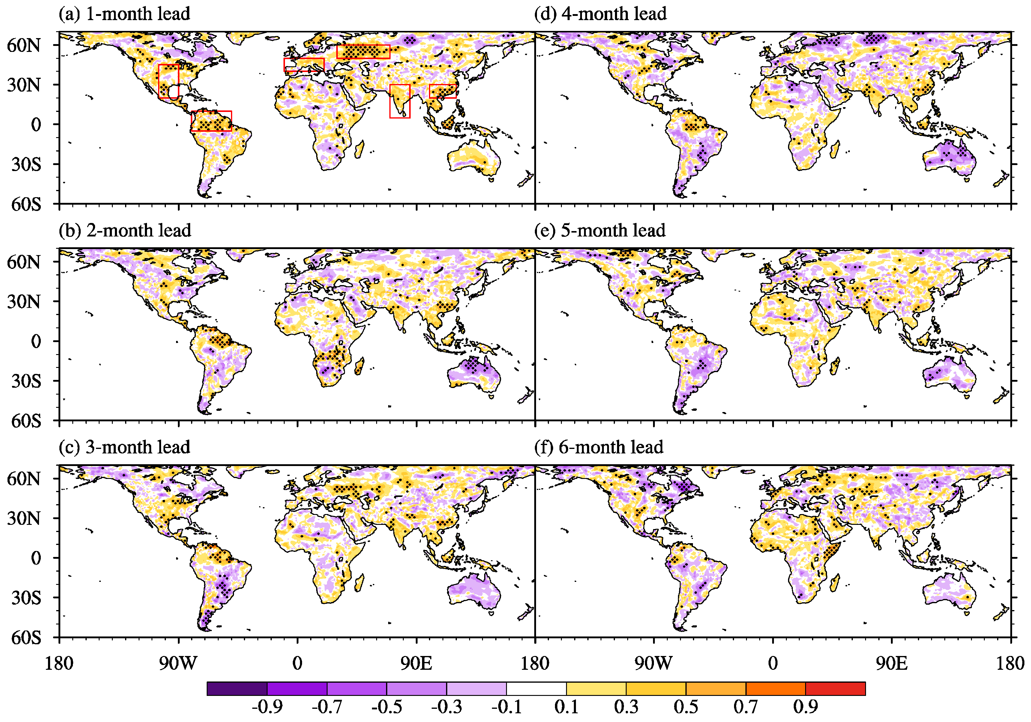
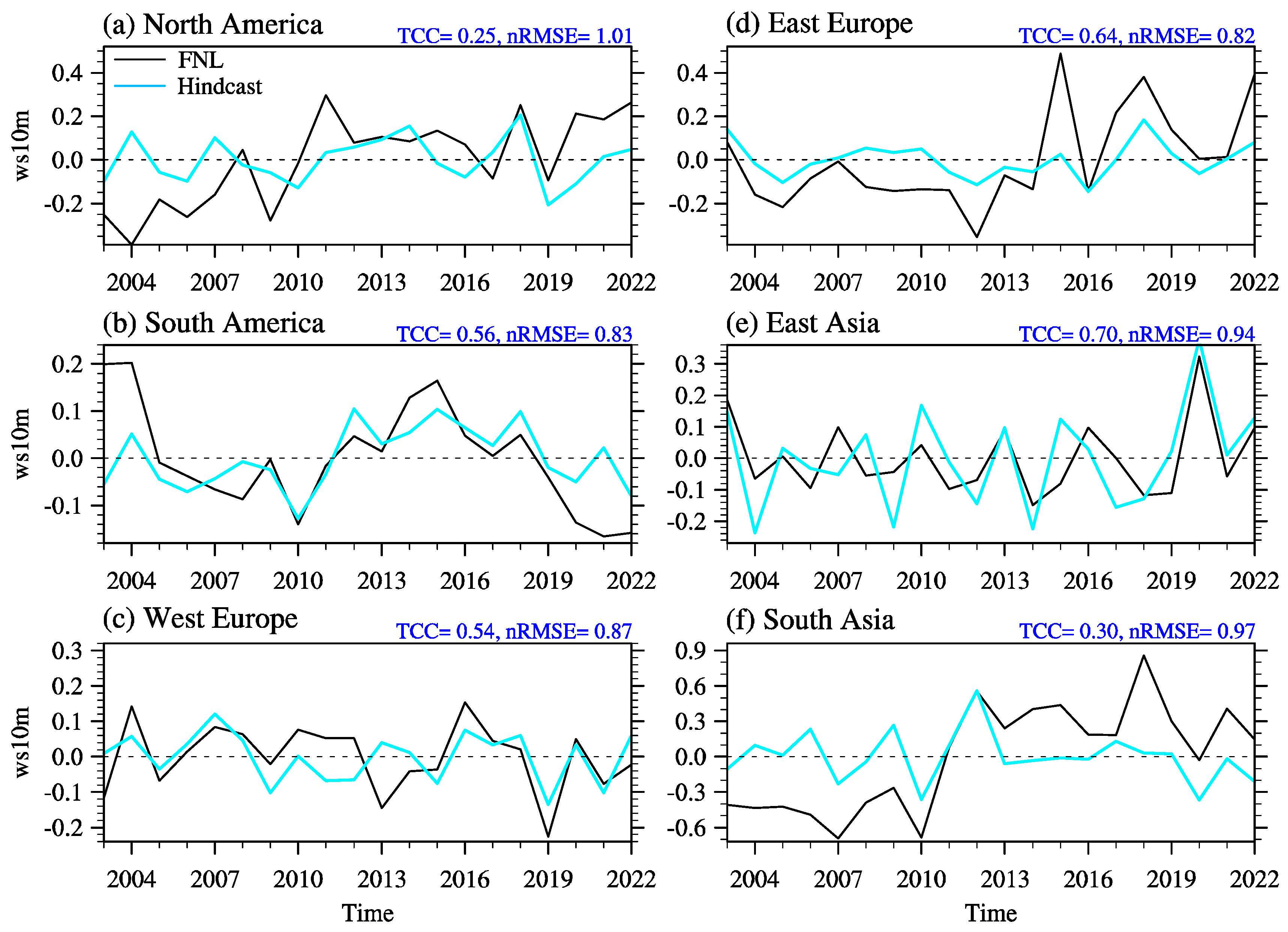
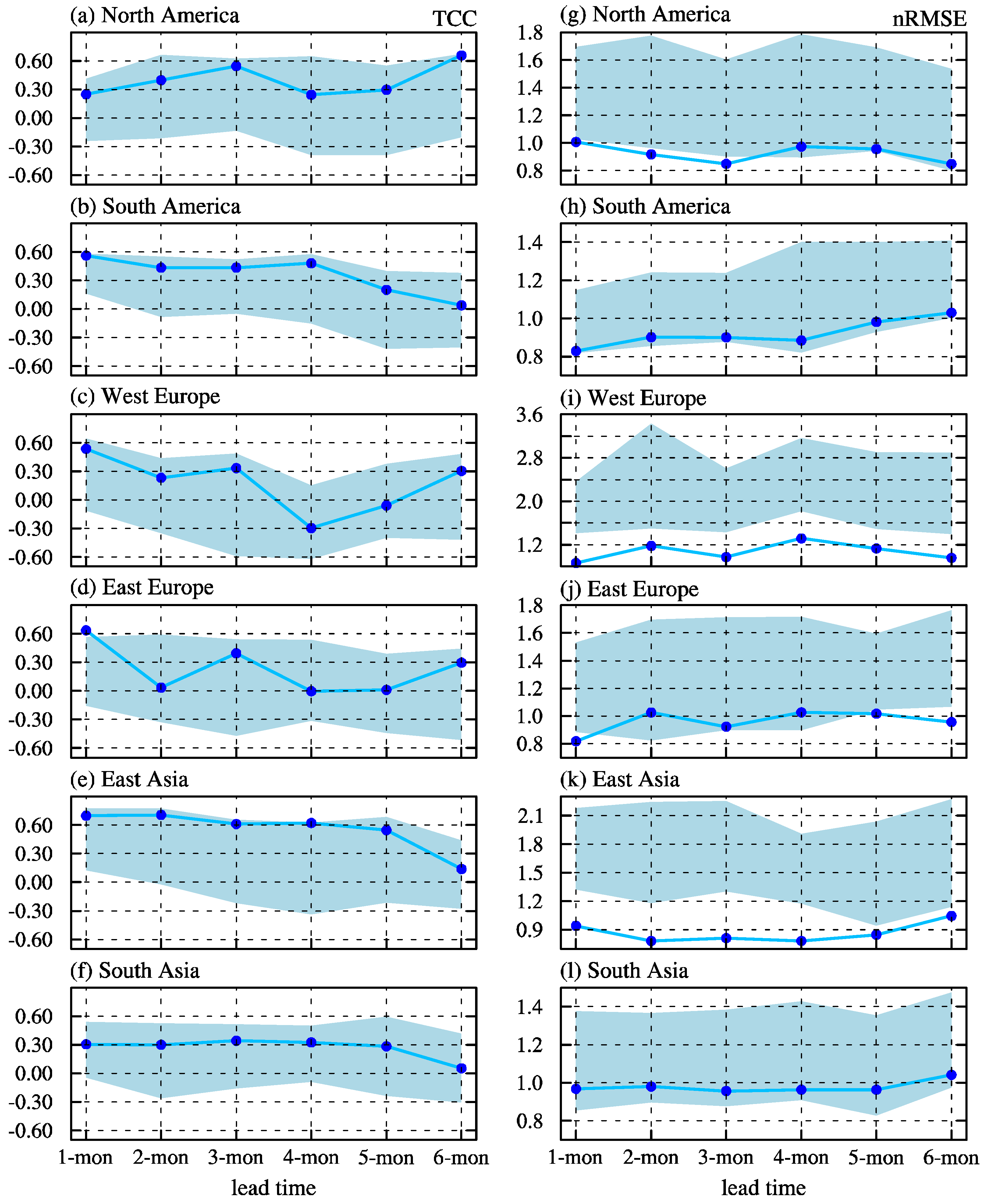
3.2. Seasonal Prediction Skill for 10 m Wind Speed

The spatial distributions of the TCC skill of JJA-mean ws10m anomalies between FNL and MME of the hindcasts with 1-month to 6-month lead times during the period of 2003–2022 are shown in Figure 3. The results show a high TCC skill for terrestrial ws10m in most regions at a 1-month lead time (Figure 3a); in particular, SIDRI-ESS V1.0 shows statistically significant positive TCC over western Canada, America, Mexico, northern South America, eastern Europe, western Europe, South Asia, East Asia, and the Maritime Continent (Figure 3a). However, the distributions of the TCC skill are uneven on a global scale as lead time increases. There are limitations on prediction skill for ws10m in some regions such as eastern Canada and Australia, where negative TCC dominates at most lead times. Some regions show a prediction skill only with a specific lead time. For example, a significant positive TCC value (TCC > 0.7) over southern Africa (10° S–20° S) appears only with a 2-month lead time, and a significant positive TCC value (TCC > 0.7) over eastern Africa appears only with a 6-month lead time. In general, six regions show considerable predictability with a 1-month to 6-month lead time (Table 2): southern North America (20° N–45° N, 105° W–90° W), northern South America (5° S–10° N, 80° W–50° W), western Europe (40° N–50° N, 10° W–20° E), eastern Europe (50° N–60° N, 30° E–70° E), South Asia (5° N–30° N, 70° E–85° E), and East Asia (20° N–30° N, 100° E–120° E) (denoted in red boxes in Figure 3a).
We also calculate the nRMSE for JJA-mean ws10m anomalies, which measures the deviation between FNL and MME of the hindcasts, regardless of the effect of magnitude. The nRMSE is greater than 1.0 in most regions at all lead times, especially in Africa and most of South and North America. It is worth noting that a relatively low nRMSE value is also found in the six regions as mentioned above, basically remaining below 0.9 (Figure 4 and Table 3). At the same time, these six regions either already have a considerable wind power industry (such as southern North America, western Europe, and South and East Asia), or have rich wind resources and are in urgent need of wind power industry deployment in the future (such as northern South America and eastern Europe) [6]. Thus, we focus on discussing the prediction skill for these regions in the following sections.
Figure 5 displays the temporal evolution of area-averaged JJA-mean ws10m anomalies for these six regions from FNL and MME of the hindcasts at a 1-month lead time. For southern North America, JJA-mean ws10m anomalies show a significant increasing trend in observations. However, this trend is not reproduced in the hindcasts, with the TCC between observations and hindcasts only 0.25, and the nRMSE reaching 1.01. This is because the hindcasts overestimate ws10m in this region before 2010; if only the temporal evolution of ws10m from 2010 to 2022 is considered, the TCC can reach 0.45 and the nRMSE can be reduced to 0.96. The observed ws10m anomalies over northern South America exhibit a decadal-like oscillation, with positive phases occurring before 2005 and from 2011 to 2019, transitioning to negative phases from 2005 to 2011 and after 2019. This phenomenon can be accurately simulated in the hindcasts, with a TCC of 0.56 and nRMSE of only 0.83. The time series of ws10m over western and eastern Europe are also well predicted in the hindcasts, with the TCC reaching 0.54 and 0.64, respectively. Meanwhile, the hindcasts show the best seasonal prediction skill for ws10m over East Asia. The temporal evolution of ws10m in the hindcasts not only matches well with the observations, but the amplitude of ws10m is basically consistent with the observations, and the TCC can reach about 0.7. However, the TCC skill in South Asia is relatively low, reaching only 0.3, similar to southern North America. The TCC significantly improves to 0.62 during the period of 2010–2022. The above results show that SIDRI-ESS V1.0 has a high seasonal prediction skill for wind speed in regions where the wind power industry is developed or will develop, which can effectively help the industry optimize and improve resource utilization, operation management, and policy formulation to improve overall economic benefits and sustainable development. For instance, Italy, Switzerland, and other European countries experienced severe heat waves in the summer of 2015, leading to a surge in local electricity demand [42]. Accurate seasonal prediction of wind speed enables the wind power industry to make generation plans and pricing strategies, ensuring a stable power supply, thus improving public service quality and maximizing economic benefits (Figure 5c).
To reduce the uncertainty in seasonal predictions, SIDRI-ESS V1.0 is a dynamic prediction system with 24 ensemble members and ensemble prediction. Figure 6 and Figure 7 display the effect of ensemble prediction on the seasonal prediction skill for ws10m. The TCC and nRMSE skill scores for six key regions at various lead times are shown in Figure 6. The region with the highest TCC skill is East Asia (TCC is greater than or close to 0.6 with a 1-month to 5-month lead time), while the lowest skill is South Asia (TCC remains 0.3) in the MME of the hindcasts. In most regions, the TCC skill diminishes as the lead time increases, except for southern North America. There, the highest prediction skill is at a 6-month lead time, which indicates that predictions with initialization in December of the previous year are the most reliable for the following summer wind speed in this region (Figure 6a). For western and eastern Europe, an effective TCC skill occurs with 1-month, 3-month, and 6-month lead times (Figure 6c,d). The light blue shading in Figure 6 shows the ensemble member spread, representing the uncertainty of the prediction. We find that ensemble prediction effectively reduces the uncertainty, and the result of the multi-member ensemble mean (blue dots and lines in Figure 6) is always close to or even greater than the individual ensemble member with the best performance. This significantly improves the deterministic prediction skill for wind speed. The results for nRMSE are similar to those for TCC, and nRMSE basically increases as lead time increases. Good correspondence is found between nRMSE and TCC; typically, higher TCC accompanies smaller nRMSE. Furthermore, the effect of ensemble prediction is more noticeable in nRMSE, especially in southern North America, western and eastern Europe, and East Asia (Figure 6g–l).
Prediction skill is also influenced by ensemble size [43,44]. The impact of ensemble size on the performance of SIDRI-ESS V1.0 is analyzed in Figure 7. The TCC skill increases as the ensemble size enlarges in most regions with most lead times (Figure 7a–f). There are exceptions, such as the TCC for ws10m over western and eastern Europe with 4-month and 5-month lead times, which significantly decreases as the number of ensemble members increases (Figure 7c,d). Twenty-four ensemble members are almost sufficient to saturate the TCC skill in these six key regions with a 1-month to 5-month lead time. However, the 24 members are insufficient for the hindcast initialization in December (6-month lead, dark blue lines in Figure 7a–f), indicating the need for a further increase in ensemble size. Increasing the ensemble size significantly reduces the nRMSE, which decreases rapidly when the ensemble size enlarges from 2 to 10 members at all lead times. Moreover, 16–18 ensemble members are sufficient to minimize the nRMSE of ws10m in the six regions at all lead times (Figure 7g–l).

3.3. Seasonal Prediction for Wind Energy Generation

Previously, we discussed the seasonal prediction of wind speed; however, it is necessary to convert wind speed into wind energy for practical applications. This conversion is especially crucial for short-term forecasts, as it provides direct information for estimating the power output and efficiency of wind farms. Similarly, seasonal prediction for wind energy generation is also important for seasonal wind energy planning and power trading. In this section, we use wind power density (WPD) to represent wind energy generation, written as a function of air density ( ρ ) and the cube of 10 m wind speed (U):
W P D = 1 2 ρ U 3
First, we investigate the extent to which wind speed can represent wind energy on a seasonal timescale. Figure 8 illustrates the correlation coefficient between the JJA-mean ws10m and JJA-mean WPD for both observations and hindcasts. In the observations, the correlation coefficient is generally above 0.5 over global land, except for part of central South America, and the highest correlations appear mainly in the tropics (20° S–20° N) (Figure 8a). The results of the hindcasts are basically consistent with the observations, except for the eastern USA, where there is a negative correlation at all lead times (Figure 8b–g). Notably, the correlation between ws10m and WPD is negative in most regions north of 20° N in the Northern Hemisphere at a 2-month lead time. This suggests that wind energy generation is strongly correlated with wind speed in most regions, but wind speed may not fully represent wind energy in certain regions at specific lead times.
Furthermore, we evaluate the direct seasonal prediction skill for WPD in SIDRI-ESS V1.0. The prediction skill for WPD is slightly lower than that for ws10m (Figure 6 and Figure 9), as indicated by the lower (higher) TCC (nRMSE) for WPD compared with ws10m in southern North America, western Europe, eastern Europe, and East Asia at almost all lead times. Additionally, the prediction skill for WPD in South Asia is highly consistent with the skill for ws10m (Figure 6f,l and Figure 9f,l), due to the strong correlation between WPD and ws10m (Figure 8). However, the TCC skill for WPD in South America is slightly higher than that for ws10m, with the TCC value remaining at 0.6 from a 1-month to 6-month lead time (Figure 6b and Figure 9b). This indicates that WPD can more accurately represent the wind resources in this region than wind speed.

4. Summary and Discussion

The seasonal prediction skill for global onshore wind resources is evaluated using the SIDRI-ESS V1.0 dynamic prediction system, developed by the Shanghai Investigation Design and Research Institute Co., Ltd. (Shanghai, China) SIDRI-ESS V1.0 is designed based on a fully-coupled global climate model, with only atmospheric assimilation being currently conducted. Twenty-year hindcasts with 24 ensemble members are conducted based on SIDRI-ESS V1.0. In this study, we focus on the prediction skill for wind resources during boreal summer. The major conclusions are summarized as follows.
We first analyze the simulation of climatological 10 m wind speed in SIDRI-ESS V1.0. The hindcasts generally overestimate the climatological wind speed in most regions, and the results are consistent at all lead times. The biases in the hindcasts are much lower than those in the free-coupled experiment, due to the contribution of data assimilation in SIDRI-ESS V1.0, which effectively reduces the influence of model drift.
The seasonal prediction skill for global onshore wind resources in SIDRI-ESS V1.0 is quantitatively evaluated using the temporal correlation coefficient (TCC) and normalized root mean square error (nRMSE). High and stable prediction skill is observed in six regions, including southern North America, northern South America, western and eastern Europe, and South and East Asia, where the wind power industry has been developed or there are rich wind resources and an urgent need for wind power industry deployment in the future. The prediction skill for East Asia is the highest, and effective prediction of summer wind resources in East Asia can be produced 5 months in advance. For most regions, the prediction skill diminishes with increased lead time. However, there are exceptions; the skill for southern North America reaches a maximum at a 6-month lead time.
Additionally, we highlight the importance of ensemble prediction for the predictive skill of wind resources, which significantly reduces uncertainty and improves the deterministic prediction skill. This is also evidenced by the fact that the results from the multi-model ensemble mean are always close to or even surpass the performance of the best individual ensemble member. Increasing the ensemble size generally improves the prediction skill, and the optimal number of ensemble members varies by region and lead time, with 24 ensemble members generally sufficient to saturate the TCC and nRMSE skill scores for most regions and lead times. However, the current scale is insufficient for achieving maximum prediction skill at a 6-month lead time, indicating the need for a further increase in ensemble size to improve prediction skill.
Furthermore, we explore whether 10 m wind speed can represent other wind resources, such as wind power density (WPD). WPD shows a strong correlation with 10 m wind speed globally in both observations and SIDRI-ESS V1.0, especially in tropical regions. This indicates that wind speed can effectively represent wind resources in most regions. The direct seasonal prediction skill for WPD is slightly lower than that for wind speed in most regions. The prediction skill for northern South America even surpasses that for wind speed at all lead times, suggesting that wind power density may be a more effective measure for this region.
Overall, SIDRI-ESS V1.0 shows skillful seasonal prediction of global onshore wind resources, particularly in regions where the wind power industry is well developed or has development potential. However, its predictive skill still shows limitations in some areas with rich wind resources (such as eastern Brazil and northern Australia). In the future, the combination of AI algorithms is expected to further improve prediction skills [32,45,46,47]. Additionally, it is also important to consider the connections between seasonal prediction results and wind power plants, as well as power supply systems, to optimize resource utilization, operation management, and policy formulation for the wind power industry, especially in hard-to-reach conditions [48,49].

Author Contributions

Author Contributions: Conceptualization, Z.Y. and W.Z.; Methodology, Z.Y. and J.L.; Formal analysis, Z.Y. and Y.Z.; Writing—original draft, Z.Y., W.Z. and J.L.; Writing—review & editing, Z.Y., W.Z., J.L., X.Z. and L.Z. All authors have read and agreed to the published version of the manuscript.

Funding

This research was funded by the National Natural Science Foundation of China (grant number 42288101, 42361144708, 42192563 and 42120104001). And the APC was funded by the Shanghai Investigation Design and Research Institute Co., Ltd. (Shanghai, China).

Institutional Review Board Statement

Not applicable.

Informed Consent Statement

Not applicable.

Data Availability Statement

The data presented in this research may be requested from authors.

Conflicts of Interest

Authors Zixiang Yan, Jinxiao Li, Xuedan Zhu, Yuxin Zang and Liuyi Zhang were employed by the company Shanghai Investigation, Design and Research Institute Co., Ltd. The remaining author declares that the research was conducted in the absence of any commercial or financial relationships that could be construed as a potential conflict of interest.

References

  1. Barthelmie, R.J.; Pryor, S.C. Potential contribution of wind energy to climate change mitigation. Nat. Clim. Chang. 2014, 4, 684–688. [Google Scholar] [CrossRef]
  2. Bonou, A.; Laurent, A.; Olsen, S.I. Life cycle assessment of onshore and offshore wind energy-from theory to application. Appl. Energy 2016, 180, 327–337. [Google Scholar] [CrossRef]
  3. GWEC. Global Wind Report 2022; Global Wind Energy Council: Brussels, Belgium, 2023. [Google Scholar]
  4. Roulston, M.S.; Kaplan, D.T.; Hardenberg, J.; Smith, L.A. Using medium-range weather forcasts to improve the value of wind energy production. Renew. Energy 2003, 28, 585–602. [Google Scholar] [CrossRef]
  5. Clark, R.T.; Bett, P.E.; Thornton, H.E.; Scaife, A.A. Skilful seasonal predictions for the European energy industry. Environ. Res. Lett. 2017, 12, 024002. [Google Scholar] [CrossRef]
  6. Torralba, V.; Doblas-Reyes, F.J.; MacLeod, D.; Christel, I.; Davis, M. Seasonal Climate Prediction: A New Source of Information for the Management of Wind Energy Resources. J. Appl. Meteorol. Climatol. 2017, 56, 1231–1247. [Google Scholar] [CrossRef]
  7. White, C.J.; Carlsen, H.; Robertson, A.W.; Klein, R.J.T.; Lazo, J.K.; Kumar, A.; Vitart, F.; Coughlan de Perez, E.; Ray, A.J.; Murray, V.; et al. Potential applications of subseasonal-to-seasonal (S2S) predictions. Meteorol. Appl. 2017, 24, 315–325. [Google Scholar] [CrossRef]
  8. Staffell, I.; Pfenninger, S. The increasing impact of weather on electricity supply and demand. Energy 2018, 145, 65–78. [Google Scholar] [CrossRef]
  9. Orlov, A.; Sillmann, J.; Vigo, I. Better seasonal forecasts for the renewable energy industry. Nat. Energy 2020, 5, 108–110. [Google Scholar] [CrossRef]
  10. Wiatros-Motyka, M.; Fulghum, N.; Jones, D. Global Electricity Review 2024; Ember: Atlanta, GA, USA, 2024. [Google Scholar]
  11. EI. Energy Institute Statistical Review of World Energy 2024; EI: Tokyo, Japan, 2024. [Google Scholar]
  12. Lange, B.; Rohrig, K.; Ernst, B. Wind power forecasting in Germany—Recent advances and future challenges. Z. Für Energiewirtschaft 2006, 30, 115–120. [Google Scholar]
  13. De Giorgi, M.G.; Ficarella, A.; Tarantino, M. Error analysis of short term wind power prediction models. Appl. Energy 2011, 88, 1298–1311. [Google Scholar] [CrossRef]
  14. Wang, Y.; Zou, R.; Liu, F.; Zhang, L.; Liu, Q. A review of wind speed and wind power forecasting with deep neural networks. Appl. Energy 2021, 304, 117766. [Google Scholar] [CrossRef]
  15. Foley, A.M.; Leahy, P.G.; Marvuglia, A.; McKeogh, E.J. Current methods and advances in forecasting of wind power generation. Renew. Energy 2012, 37, 1–8. [Google Scholar] [CrossRef]
  16. Enloe, J.; O’Brien, J.J.; Smith, S.R. ENSO Impacts on Peak Wind Gusts in the United States. J. Clim. 2004, 17, 1728–1737. [Google Scholar] [CrossRef]
  17. Brayshaw, D.J.; Troccoli, A.; Fordham, R.; Methven, J. The impact of large scale atmospheric circulation patterns on wind power generation and its potential predictability: A case study over the UK. Renew. Energy 2011, 36, 2087–2096. [Google Scholar] [CrossRef]
  18. Hamlington, B.D.; Hamlington, P.E.; Collins, S.G.; Alexander, S.R.; Kim, K.-Y. Effects of climate oscillations on wind resource variability in the United States. Geophys. Res. Lett. 2015, 42, 145–152. [Google Scholar] [CrossRef]
  19. Sherman, P.; Chen, X.; McElroy, M.B. Wind-generated Electricity in China: Decreasing Potential, Inter-annual Variability and Association with Changing Climate. Sci. Rep. 2017, 7, 16294. [Google Scholar] [CrossRef]
  20. Xu, Q.; Chen, W.; Song, L. Two Leading Modes in the Evolution of Major Sudden Stratospheric Warmings and Their Distinctive Surface Influence. Geophys. Res. Lett. 2022, 49, e2021GL095431. [Google Scholar] [CrossRef]
  21. Bett, P.E.; Thornton, H.E.; Lockwood, J.F.; Scaife, A.A.; Golding, N.; Hewitt, C.; Zhu, R.; Zhang, P.; Li, C. Skill and Reliability of Seasonal Forecasts for the Chinese Energy Sector. J. Appl. Meteorol. Climatol. 2017, 56, 3099–3114. [Google Scholar] [CrossRef]
  22. Lee, D.Y.; Doblas-Reyes, F.J.; Torralba, V.; Gonzalez-Reviriego, N. Multi-model seasonal forecasts for the wind energy sector. Clim. Dyn. 2019, 53, 2715–2729. [Google Scholar] [CrossRef]
  23. Lockwood, J.F.; Thornton, H.E.; Dunstone, N.; Scaife, A.A.; Bett, P.E.; Li, C.; Ren, H.-L. Skilful seasonal prediction of winter wind speeds in China. Clim. Dyn. 2019, 53, 3937–3955. [Google Scholar] [CrossRef]
  24. Soret, A.; Torralba, V.; Cortesi, N.; Christel, I.; Palma, L.; Manrique-Suñén, A.; Lledó, L.; González-Reviriego, N.; Doblas-Reyes, F.J. Sub-seasonal to seasonal climate predictions for wind energy forecasting. J. Phys. Conf. Ser. 2019, 1222, 012009. [Google Scholar] [CrossRef]
  25. Zeng, P.; Sun, X.; Farnham, D.J. Skillful statistical models to predict seasonal wind speed and solar radiation in a Yangtze River estuary case study. Sci. Rep. 2020, 10, 8597. [Google Scholar] [CrossRef] [PubMed]
  26. Bett, P.E.; Thornton, H.E.; Troccoli, A.; De Felice, M.; Suckling, E.; Dubus, L.; Saint-Drenan, Y.-M.; Brayshaw, D.J. A simplified seasonal forecasting strategy, applied to wind and solar power in Europe. Clim. Serv. 2022, 27, 100318. [Google Scholar] [CrossRef]
  27. Lockwood, J.F.; Stringer, N.; Hodge, K.R.; Bett, P.E.; Knight, J.; Smith, D.; Scaife, A.A.; Patterson, M.; Dunstone, N.; Thornton, H.E. Seasonal prediction of UK mean and extreme winds. Q. J. R. Meteorol. Soc. 2023, 149, 3477–3489. [Google Scholar] [CrossRef]
  28. Yang, X.; Delworth, T.L.; Jia, L.; Johnson, N.C.; Lu, F.; McHugh, C. Skillful seasonal prediction of wind energy resources in the contiguous United States. Commun. Earth Environ. 2024, 5, 313. [Google Scholar] [CrossRef]
  29. Troccoli, A.; Goodess, C.; Jones, P.; Penny, L.; Dorling, S.; Harpham, C.; Dubus, L.; Parey, S.; Claudel, S.; Khong, D.H.; et al. Creating a proof-of-concept climate service to assess future renewable energy mixes in Europe: An overview of the C3S ECEM project. Adv. Sci. Res. 2018, 15, 191–205. [Google Scholar] [CrossRef]
  30. Pan, B.; Anderson, G.J.; Goncalves, A.; Lucas, D.D.; Bonfils, C.J.W.; Lee, J. Improving Seasonal Forecast Using Probabilistic Deep Learning. J. Adv. Model. Earth Syst. 2022, 14, e2021MS002766. [Google Scholar] [CrossRef]
  31. El-Azab, H.A.; Swief, R.; El-Amary, N.; Temraz, H. Seasonal Forecasting of Wind and Solar Power Using Deep Learning Algorithms. In Proceedings of the 2023 24th International Middle East Power System Conference (MEPCON), Mansoura, Egypt, 19–21 December 2023; pp. 1–8. [Google Scholar]
  32. Tong, X.; Zhou, W.; Xia, J. Improving Boreal Summer Precipitation Predictions From the Global NMME Through Res34-Unet. Geophys. Res. Lett. 2024, 51, e2023GL106391. [Google Scholar] [CrossRef]
  33. National Centers for Environmental Prediction/National Weather Service/NOAA/U.S. Department of Commerce, 2000: NCEP FNL Operational Model Global Tropospheric Analyses, Continuing from July 1999. Research Data Archive at the National Center for Atmospheric Research, Computational and Information Systems Laboratory. 19 July. Available online: https://doi.org/10.5065/D6M043C6 (accessed on 27 March 2023).
  34. Lin, S.-J. A “Vertically Lagrangian” Finite-Volume Dynamical Core for Global Models. Mon. Weather Rev. 2004, 132, 2293–2307. [Google Scholar] [CrossRef]
  35. Putman, W.M.; Lin, S.-J. Finite-volume transport on various cubed-sphere grids. J. Comput. Phys. 2007, 227, 55–78. [Google Scholar] [CrossRef]
  36. Smith, R.D.; Jones, P.; Briegleb, B.; Bryan, F.; Danabasoglu, G.; Dennis, J.; Dukowicz, J.; Eden, C.; Fox-Kemper, B.; Gent, P.; et al. The Parallel Ocean Program (POP) Reference Manual; Technical Report for Los Alamos National Labora-tory LAUR-10-01853; Los Alamos National Laboratory: Los Alamos, NM, USA, 2010; p. 140. [Google Scholar]
  37. Oleson, K.W.; Lawrence, D.M.; Gordon, B.; Flanner, M.G.; Kluzek, E.; Peter, J.; Levis, S.; Swenson, S.C.; Thornton, E.; Feddema, J. Technical Description of Version 4.0 of the Community land Model (CLM); National Center for At-mospheric Research: Boulder, CO, USA, 2010. [Google Scholar]
  38. Hunke, E.; Lipscomb, W. CICE: The Los Alamos Sea Ice Model Documentation and Software User’s Manual Version 4.0; Tech. Rep. LA–CC–06–012; Los Alamos National Laboratory: Los Alamos, NM, USA, 2010. [Google Scholar]
  39. Bloom, S.C.; Takacs, L.L.; da Silva, A.M.; Ledvina, D. Data Assimilation Using Incremental Analysis Updates. Mon. Weather Rev. 1996, 124, 1256–1271. [Google Scholar] [CrossRef]
  40. Magnusson, L.; Alonso-Balmaseda, M.; Corti, S.; Molteni, F.; Stockdale, T. Evaluation of forecast strategies for seasonal and decadal forecasts in presence of systematic model errors. Clim. Dyn. 2013, 41, 2393–2409. [Google Scholar] [CrossRef]
  41. Wang, C.; Zhang, L.; Lee, S.-K.; Wu, L.; Mechoso, C.R. A global perspective on CMIP5 climate model biases. Nat. Clim. Chang. 2014, 4, 201–205. [Google Scholar] [CrossRef]
  42. Russo, S.; Sillmann, J.; Fischer, E.M. Top ten European heatwaves since 1950 and their occurrence in the coming decades. Environ. Res. Lett. 2015, 10, 124003. [Google Scholar] [CrossRef]
  43. Buizza, R.; Palmer, T.N. Impact of Ensemble Size on Ensemble Prediction. Mon. Weather Rev. 1998, 126, 2503–2518. [Google Scholar] [CrossRef]
  44. Ma, J.; Zhu, Y.; Wobus, R.; Wang, P. An effective configuration of ensemble size and horizontal resolution for the NCEP GEFS. Adv. Atmos. Sci. 2012, 29, 782–794. [Google Scholar] [CrossRef]
  45. Han, Y.; Mi, L.; Shen, L.; Cai, C.S.; Liu, Y.; Li, K.; Xu, G. A short-term wind speed prediction method utilizing novel hybrid deep learning algorithms to correct numerical weather forecasting. Appl. Energy 2022, 312, 118777. [Google Scholar] [CrossRef]
  46. Tong, X.; Li, J.; Zhang, F.; Li, W.; Pan, B.; Li, J.; Letu, H. The Deep-Learning-Based Fast Efficient Nighttime Retrieval of Thermodynamic Phase From Himawari-8 AHI Measurements. Geophys. Res. Lett. 2023, 50, e2022GL100901. [Google Scholar] [CrossRef]
  47. Zhao, J.; Guo, Y.; Lin, Y.; Zhao, Z.; Guo, Z. A novel dynamic ensemble of numerical weather prediction for multi-step wind speed forecasting with deep reinforcement learning and error sequence modeling. Energy 2024, 302, 131787. [Google Scholar] [CrossRef]
  48. Klyuev, R.; Bosikov, I.; Gavrina, O. Use of Wind Power Stations for Energy Supply to Consumers in Mountain Territories. In Proceedings of the 2019 International Ural Conference on Electrical Power Engineering (UralCon), Chelyabinsk, Russia, 1–3 October 2019; pp. 116–121. [Google Scholar]
  49. Han, J.; Wang, X.; Yang, X.; Ling, Q.; Liu, W. Yaw system restart strategy optimization of wind turbines in mountain wind farms based on operational data mining and multi-objective optimization. Eng. Appl. Artif. Intell. 2023, 126, 107036. [Google Scholar] [CrossRef]
Figure 1. JJA-mean climatological 10 m wind speed (ws10m, units: m/s) in FNL and model biases during 2003–2022. (a) JJA-mean climatological ws10m in FNL. (b) Bias between the free-coupled experiment and FNL. (c) Bias between the nudging experiment and FNL.
Sustainability 16 07721 g001
Figure 2. Spatial distribution of biases of JJA-mean climatological ws10m between hindcasts and FNL with a 1-month to 6-month lead time, respectively.
Sustainability 16 07721 g002
Figure 3. Spatial distribution of the temporal correlation coefficient (TCC) of JJA-mean ws10m anomalies between the hindcasts and FNL over the period 2003–2022 with a 1-month to 6-month lead time. Values reaching the 10% significance level are dotted in black. The red boxes in (a) are North America (20° N–45° N, 105° W–90° W), South America (5° S–10° N, 80° W–50° W), western Europe (40° N–50° N, 10° W–20° E), eastern Europe (50° N–60° N, 30° E–70° E), East Asia (20° N–30° N, 100° E–120° E), and South Asia (5° N–30° N, 70° E–85° E), respectively.
Sustainability 16 07721 g003
Figure 4. Spatial distribution of normalized root mean square error (nRMSE) of JJA-mean ws10m anomalies between the hindcasts and FNL over the period 2003–2022 with a 1-month to 6-month lead time.
Sustainability 16 07721 g004
Figure 5. Time series of area-averaged JJA-mean onshore ws10m anomalies over six regions. Black lines are the result of FNL. Blue lines are the result of the hindcasts at a 1-month lead time. TCC and nRMSE are noted in the upper right corner.
Sustainability 16 07721 g005
Figure 6. TCC (left panel) and nRMSE (right panel) skill scores of area-averaged JJA-mean ws10m anomalies over six regions in the hindcasts. The abscissa shows the lead time in months. (a) North America. (bf) As in (a), but for South America, western Europe, eastern Europe, East Asia, and South Asia, respectively. (gl) As in (af), but for nRMSE. The dark blue dots and lines are the MME of the hindcasts. The light blue shading denotes the spread of the 24 ensemble members.
Sustainability 16 07721 g006
Figure 7. Effect of ensemble size on TCC (left panel) and nRMSE (right panel) of JJA-mean ws10m anomalies over six regions in the hindcasts. The abscissa indicates the number of ensemble members (increasing from 1 to 24). The brown, orange, peach, green, cyan, and dark blue lines denote the results with a 1-month to 6-month lead time, respectively.
Sustainability 16 07721 g007
Figure 8. Spatial distribution of the correlation coefficient between JJA-mean ws10m and JJA-mean wind power density (WPD, units: W/m2). (a) Result in FNL. (bg) As in (a), but for the result in the hindcasts with a 1-month to 6-month lead time. Values reaching the 10% significance level are dotted in black.
Sustainability 16 07721 g008
Figure 9. As in Figure 6, but for JJA-mean WPD.
Sustainability 16 07721 g009
Table 1. Summary for seasonal prediction skill for summer mean wind resources in previous studies.
CitationsForecast SystemPrediction Skill
Bett et al. [21]GloSea5Focusing on seasonal prediction for 10 m wind speed (ws10m) over China, the maximum TCC (0.58) for ws10m was found in Yunnan region at a 1-month lead time.
Lee et al. [22]ECMWF System4
Météo-France System3
Météo-France System4
Météo-France System5
Significant fair ranked probability skill score (FRPSS) for ws10m concentrates on Maritime Continent and India (values reach about 0.5).
Bett et al. [26]GloSea5
Météo-France System5
ECMWF System4
Skills are patchy among different systems over Europe with negative TCC for most regions at a 1-month lead time.
Lockwood et al. [27]GloSea5
GloSea6
Focusing on prediction skill for ws10m over UK, the TCC is only about −0.3 at a 1-month lead time.
Yang et al. [28]GFDL-SPEARFocusing on prediction skill for wind power over U.S. Great Plains, the TCC for Northern (Southern) Great Plains reach about 0.4–0.5 (0.3–0.4) at a 1-month lead time.
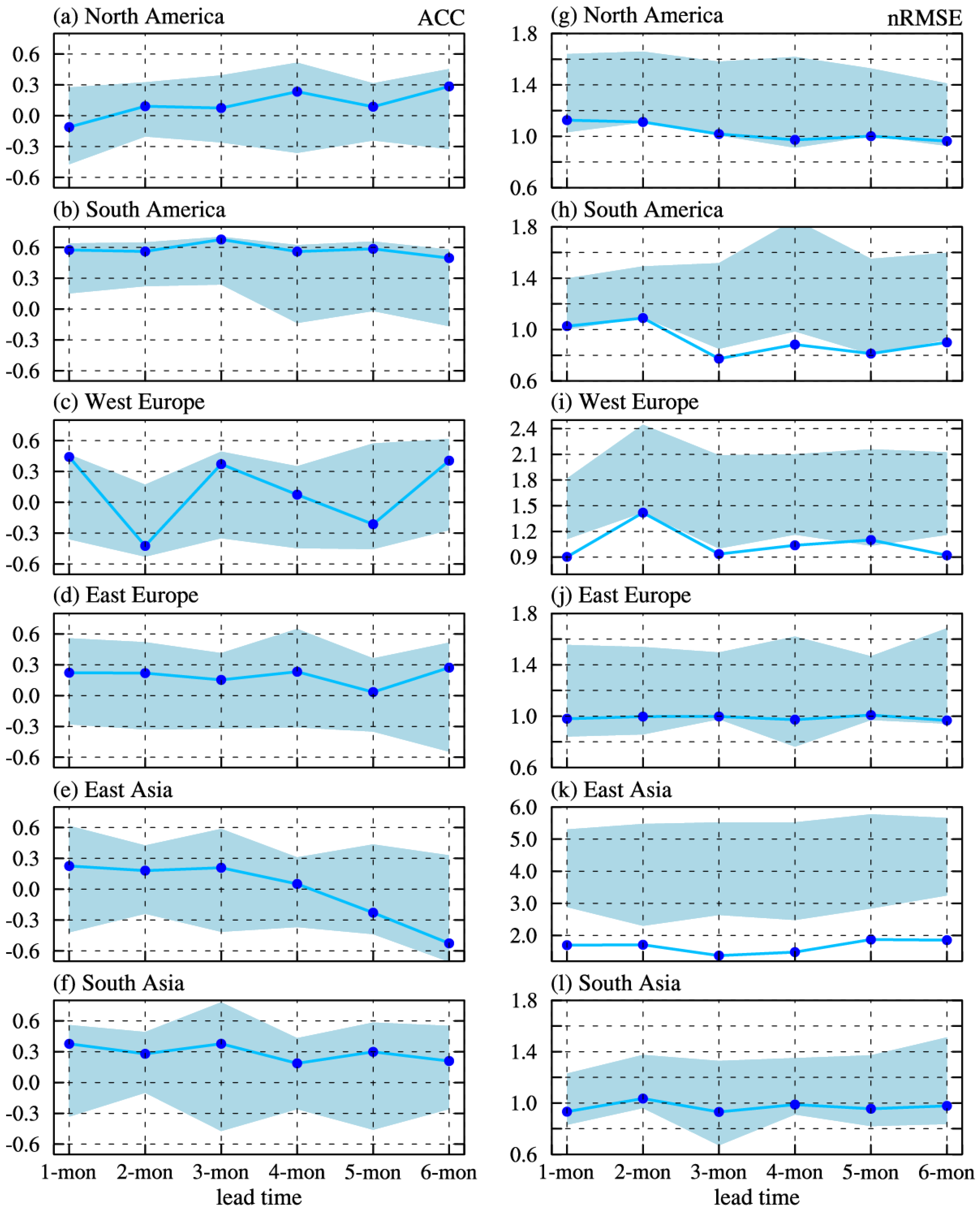
Table 2. Temporal correlation coefficient (TCC) of area-averaged JJA-mean ws10m anomalies over six regions between the multi-member ensemble of hindcasts and FNL over the period 2003–2022 with a 1-month to 6-month lead time.
Region1-Month2-Month3-Month4-Month5-Month6-Month
North America0.250.400.540.240.300.66
South America0.560.430.430.480.200.04
Western Europe0.540.230.33−0.30−0.060.30
Eastern Europe0.640.030.400.000.010.30
East Asia0.700.710.610.620.550.14
South Asia0.300.300.340.320.280.05
Table 3. As in revised Table 2, but for normalized root mean square error (nRMSE).
Region1-Month2-Month3-Month4-Month5-Month6-Month
North America1.000.920.850.970.960.85
South America0.830.900.900.880.981.03
Western Europe0.871.180.971.321.130.96
Eastern Europe0.821.030.921.031.020.96
East Asia0.940.780.810.780.851.05
South Asia0.970.980.960.960.961.04
Disclaimer/Publisher’s Note: The statements, opinions and data contained in all publications are solely those of the individual author(s) and contributor(s) and not of MDPI and/or the editor(s). MDPI and/or the editor(s) disclaim responsibility for any injury to people or property resulting from any ideas, methods, instructions or products referred to in the content.

