Simulation of Urban Carbon Sequestration Service Flows and the Sustainability of Service Supply and Demand

Abstract

Simulating ecosystem carbon sequestration service (ECSS) flows is crucial for optimizing the carbon cycle in ecosystems and achieving sustainable balance between the supply and demand of the ECSS. This study integrates least-cost path analysis with Kriging interpolation to simulate the dominant wind direction and corrects the interpolated wind speeds to account for terrain and surface conditions. Carbon emissions are spatially distributed using points of interest and road network data. Ultimately, by traversing the carbon emission rate grids along wind directions, the ECSS flows are simulated. The results reveal that the study area has a small carbon sink area but a high total carbon emission, leading to a situation where the supply of ECSS is insufficient to meet demand. The ECSS flows, based on the simulated wind field, demonstrate high spatial resolution and highlight the service flow corridors with distinct spatial heterogeneity. The study area has a significant carbon surplus, requiring a forest area ten times larger than the study area itself to fully sequester this carbon. These findings provide valuable insights for urban sustainable development and carbon emission reduction strategies.

1. Introduction

Ecosystem services (ES) primarily denote the tangible or intangible benefits that ecological systems provide to human beings, whether through direct or indirect means [1]. Numerous studies by scholars have highlighted a misalignment between the supply and demand of ES, as well as the spatial patterns in their flows [2,3]. The movement of ES from supply areas to demand areas often follows specific directions and pathways [4]. While there is no universally agreed concept or definition of ES flows within the academic community [5,6,7], it essentially delineates the process of the ES generating effect ex situ. This process establishes a vital linkage between ecosystem functions and human well-being, underscoring the intertwined nature of ES with societal needs [8,9]. ES flows are categorized into three types [4]: in situ service flows, omnidirectional service flows, and directional service flows. The current research predominantly focuses on directional physical service flows, such as water and material flows [10,11,12], whereas omnidirectional service flows, including carbon sequestration, air purification, and temperature regulation, warrant further investigation [13].

In response to global warming, nations worldwide are committed to advancing their carbon neutrality plans, undertaking voluntary measures to control and reduce carbon emissions and aiming to resolve the spatial mismatch between carbon supply and demand promptly [14]. Carbon sequestration, the process of storing CO₂ in ecosystems, plays a crucial role in climate regulation. The spatial–temporal transfer of ecosystem carbon sequestration services (ECSS) from ecosystems to humans is termed ECSS flow [15]. In this flow, carbon sources and sinks are linked by atmospheric circulation [16] and adhere to natural laws. The following problems arise in the current research on ECSS flow: (1) The studies often focus on large-scale areas such as river basins [17,18,19], urban clusters [15,16,20], and plateaus [21]. (2) The spatial resolution of ECSS flow is generally low. Two mainstream methods determine ECSS flow paths: one utilizes wind flow fields, but suffers from limited spatial data resolution, leading to coarse spatial allocation of carbon emissions, flows, and velocities [16,17]. The second method involves subjective determinations, often assuming that the study area operates as a closed system in which ES flows exclusively from supply to demand areas. Subsequently, through the utilization of spatial network models [10,22], ecological radiation force models [21,23,24], eight-directional flow models [15,25], Bayesian models [15], and other analytical frameworks, the flow of ES is elucidated. However, this approach overlooks the natural carrier-dependence of ECSS flow and the limited control humans have over atmospheric circulation. The third assumption is that the mixing and removal of CO₂ from the atmosphere are instantaneous and do not require a flow model [26]. (3) The time scale of the carbon sequestration service flow typically spans one year, encompassing the carbon emissions and carbon storage for that period. However, CO₂ can also disperse even under calm wind conditions. In monsoon climate zones, where prevailing winds occur in at least two directions annually, the CO₂ in the region does not remain localized at its source for a full year.

Wind serves as the carrier of ECSS flow, making the precise simulation of wind direction and speed crucial. Various methods exist for observing and simulating the wind environment. On-site wind measurement provides wind direction and speed at specific measurement points [27]. Wind tunnel experiments simulate gas flows by replicating wind conditions, including direction, speed, and air pressure [28]. Computational fluid dynamics (CFD) techniques solve continuous dynamic equations to model wind fields [29,30]. While these methods yield high-precision micro-scale airflow simulations, they often fall short when applied to larger scales. The majority of macro-scale wind environments characterized by continuous spatial distribution are interpolated using meteorological station observation data [31]. Traditional interpolation methods for wind speed commonly use distance-based weighting but overlook factors like land surface variations and urban structures that can influence wind speed. Scholars have begun integrating topographic undulation [32], aspect, and slope [33] to refine these interpolations. However, methodologies for correcting urban wind speeds remain underexplored. When interpolating wind direction, using the mean value from meteorological stations may result in significant alterations to the flow direction. Alternatively, capturing wind direction at specific times may not adequately represent the prevailing wind direction.

Carbon dioxide constitutes the primary component of ECSS flow, and acquiring high-resolution spatial distribution data on carbon emissions is crucial for accurately quantifying this flow of services. Studies have established that there exists a linear correlation between nighttime brightness [34] or area of light [35] and the carbon emissions of electricity consumption. The emissions from vehicle lights, powered by fossil energy consumption, are also detectable through this method [36]. However, fossil fuels encompass various types, and not all of them exhibit a strong correlation with night lighting. A prerequisite for using nighttime light data to spatialize carbon emissions is the availability of statistics on total carbon emissions and total nighttime light values across multiple sub-regions within a given area. Nevertheless, the completeness of the energy consumption statistics at the sub-regional level is often inadequate.

In conclusion, urban areas represent significant demand zones for ECSS; yet, there remains a dearth of studies focused on ECSS flow within the urban. Urban areas are typically smaller compared to previous study regions, necessitating higher spatial resolution in wind environments than the current 1 km scale allows. Moreover, traditional meteorological data interpolation methods fail to achieve the precision required for depicting fine-scale service flows. Additionally, relying on nighttime light data for spatializing energy-related carbon emissions is defective. Certain aspects of energy consumption carbon emissions remain unaccounted for, and when only a single total carbon emission value is available for the region, spatialization becomes challenging. Therefore, the objectives of this article are as follows: (1) To spatially analyze carbon emissions within the study area by utilizing point of interest (POI) data and road network data, thereby elucidating the supply and demand patterns of ECSS. (2) To simulate the prevailing wind direction using the least-cost path (LCP) analysis combined with the Kriging interpolation technique, followed by the interpolation and correction of wind speed data from meteorological stations to achieve a wind environment with high spatial resolution. (3) To develop an ECSS flow model suitable for urban scales and to identify priority ecological restoration corridors based on carbon flux. Additionally, study calculates the carbon surplus within the study area and determines the areas of different land types required to absorb this surplus. The findings of this research can serve as a reference for the spatial quantification of ECSS flows in urban areas and provide valuable insights for environmental policy making and urban planning.

2. Materials and Methods

2.1. Study Area

This paper focuses on the urban area of Shenyang (Figure 1), covering approximately 1324 km², including Heping District, Shenhe District, Dadong District, Huanggu District, Tiexi District, Yuhong District, Sujiatun District, Hunnan District, and Shenbei New District. Shenyang City, situated in the northeast of China and serving as the capital of Liaoning Province, lies between 41°11′51″~43°2′13″ north latitude and 122°25′9″~123°48′24″ east longitude. The city experiences a continental monsoon climate, characterized by higher terrain in the east and lower terrain in the west, with an average altitude of approximately 50 m. The area is predominantly covered by cultivated land and impervious surface, which make up over 90% of the total land area and act as a significant carbon source. Impervious surfaces contribute substantially to CO₂ emissions due to extensive fossil energy consumption. The limited coverage of woodland, grassland, water areas, and bare land restricts the local carbon cycle capacity, necessitating reliance on atmospheric circulation to transport CO₂ to distant carbon sink regions. Adjacent to the east of Shenyang City, Changbai Mountain stands as a national nature reserve renowned for its intricate forest ecosystem and substantial carbon reservoir.

2.2. Data

Land use data at a spatial resolution of 30 m for the year 2022 were obtained from the Aerospace Institute [37]. Average wind speed data for 2022 were sourced from the China Meteorological Data Service Center (https://data.cma.cn/, accessed on 17 May 2024). Hourly wind direction data for the Shenyang station in 2022 were retrieved from the National Environmental Information Center (NCEI) of the National Oceanic and Atmospheric Administration (NOAA) (https://www.ncei.noaa.gov/data/global-summary-of-the-day/archive/, accessed on 6 May 2024). Chinese building height (CNBH) data were provided by the GC3S team of the School of Life Sciences at Fudan University, representing weighted average building heights at a spatial resolution of 10 m [38]. Digital Elevation Model (DEM) data were jointly measured by NASA and the National Mapping Agency (NIMA) of the Department of Defense (http://srtm.csi.cgiar.org/srtmdata/, accessed on 15 April 2024). POIs were sourced from AutoNavi Map, while road data were obtained from OpenStreetMap. Energy consumption data originated from the Shenyang Municipal Bureau of Statistics (https://tjj.shenyang.gov.cn/, accessed on 20 May 2024). Land surface temperature (LST) data were derived from the Landsat 8 surface reflectance product within the Google Earth Engine platform database.

2.3. Methods

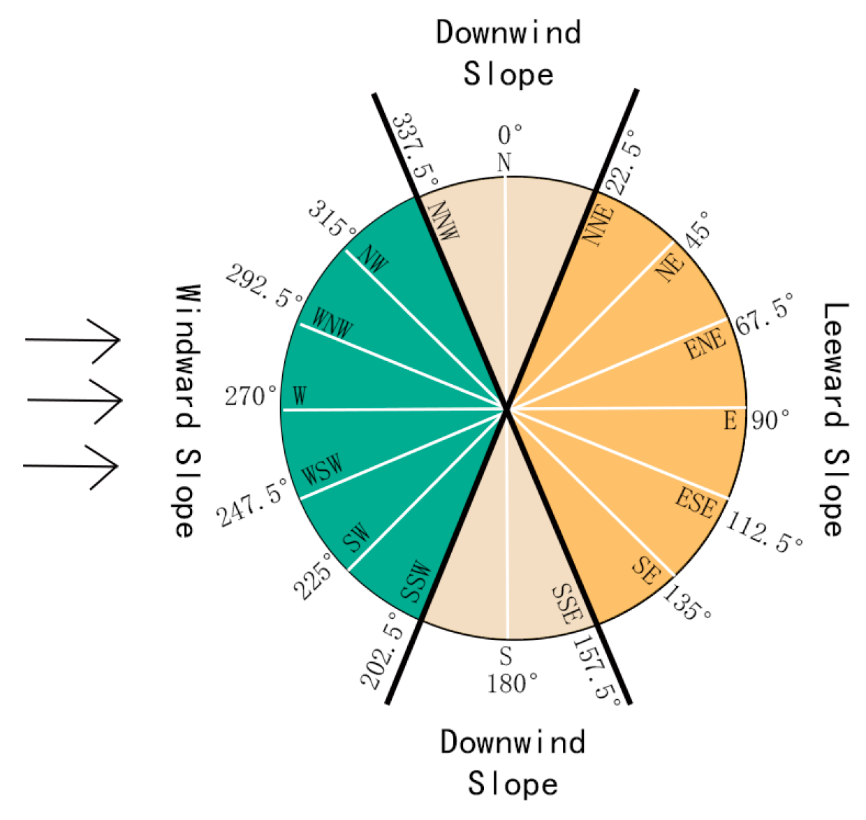
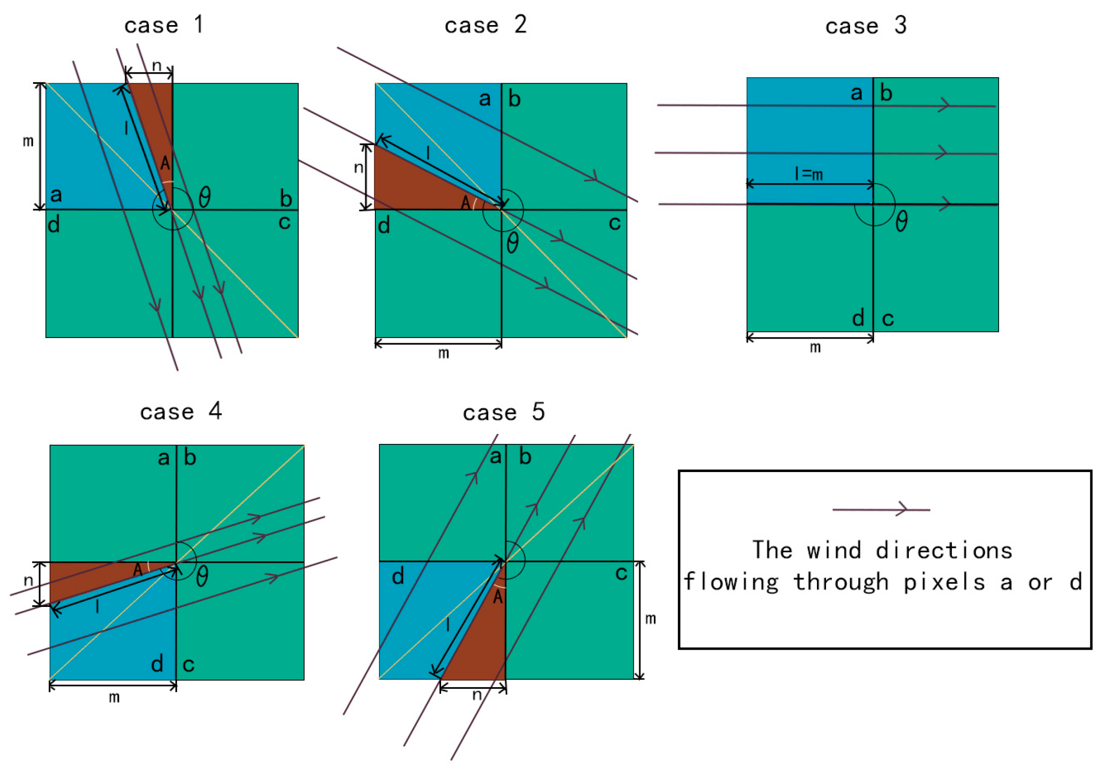
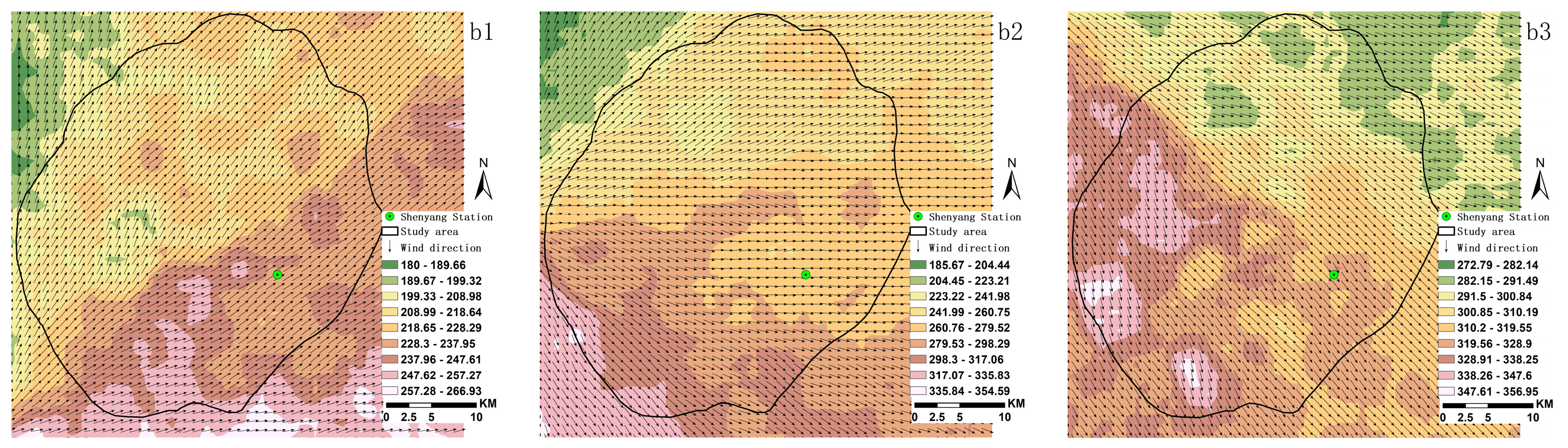
2.3.1. Interpolation of Wind Directions

Figure S1 illustrates the wind rose diagram of the Shenyang meteorological stations in 2022, predominantly from the west (including the southwesterly, westerly, and northwesterly directions). This finding is corroborated by the available literature [39] and weather data archives (https://lishi.tianqi.com/shenyang/index.html, accessed on 24 May 2024). Hence, this study identifies southwest, west, and northwest as the prevailing wind directions. Subsequently, the wind direction in the study area is simulated.

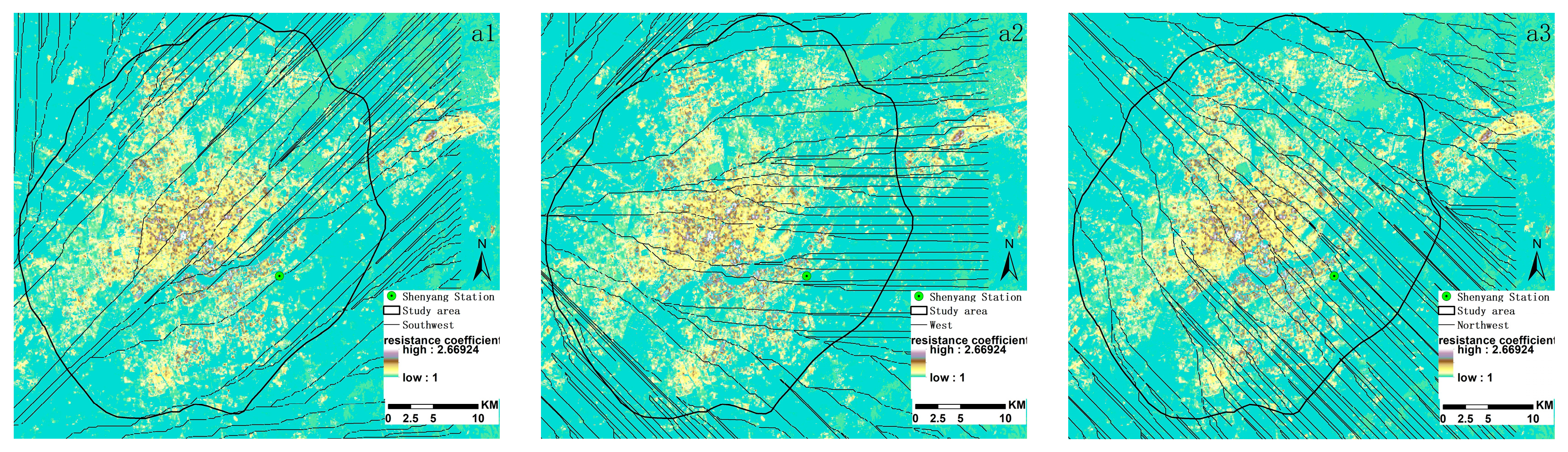
Calculate the Resistance Coefficient

The environmental impact of surface conditions and atmospheric properties causes variations in wind speed with altitude [40]. This paper adopts the logarithmic law to model the horizontal wind speed u(z) at different heights [41,42,43]:

$$u\left(z\right)=u_{*}\mathit{ln}\left(\right(z-z_d/z_0)/ k$$

(1)

where u(z) represents the horizontal wind speed at height z. u_* denotes the surface friction velocity, and k stands for the Karman constant. The surface roughness length (z₀) indicates the intercept of the vertical wind speed profile, where speed equals zero, reflecting the surface’s impact on wind speed attenuation. z_d refers to the zero plane displacement height. The parameter z_d can be approximated using Equations (S1) and (S2), used empirical coefficients z₀ [44,45], f_d [46,47,48,49,50] and f₀ [47,49,51] are shown in Table S1.

As building height increases, the phenomenon of wind shear becomes more conspicuous. Therefore, the wind resistance coefficient ξ_b can be defined as the rate of wind attenuation at the height of the ground obstacle [52].

$${\xi }_b=Q_o/Q_b$$

(2)

$$Q_b={\int }_{z_b}^{z_e}u\left(z\right)dz$$

(3)

$$Q_0={\int }_0^{z_e}u\left(z\right)dz$$

(4)

where Q_b denotes the ventilation volume from height z_b (the sum of z₀ and z_d) with zero wind speed up to the control height ze. Q₀ represents the natural ventilation volume in the absence of vegetation or building cover on the surface.

The Least-Cost Path (LCP) Analysis

The LCP analysis is widely recognized for its effectiveness in identifying potential ventilation pathways [52,53]; it offers efficient calculations to simulate near-surface wind environments by assessing underlying surface roughness [54]. Wind, being a fluid, naturally flows towards regions of lower obstruction. A smaller ξ_b indicates less resistance and lower associated costs for ventilation.

A rectangular buffer zone was established around the study area, with points placed every 1 km along the boundary of this buffer zone. The southwest, west, and northwest directions were chosen as the air inlets. All points not directly aligned in a straight line with the air inlets were designated as potential air outlets. Using the LCP analysis, potential ventilation pathways were calculated in three directions originating from the selected air inlet points.

Interpolation of Prevailing Wind Directions

The potential ventilation paths are disrupted at the turning points, where segments shorter than 150 m are removed. Subsequently, the Cartesian coordinates of each remaining line segment’s start and end points are used to calculate the angle. This angle is then converted into a wind direction angle and assigned to the midpoint of the line segment. The points from multiple ventilation paths undergo Kriging interpolation to generate an urban wind direction raster reflecting the dominant wind patterns.

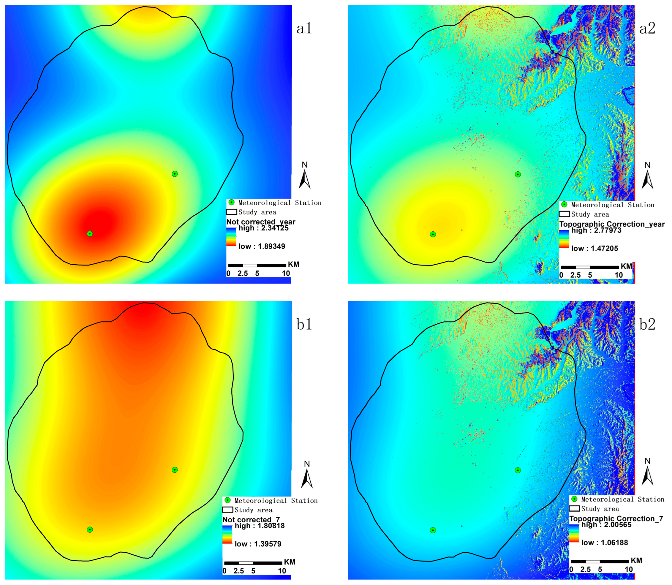
2.3.2. Interpolation and Correction of Wind Speed

Interpolation of Wind Speed

Kriging interpolation was applied to estimate the annual average wind speed (AAWS) and the July average wind speed (JAWS) at the meteorological stations. However, conventional Kriging interpolation methods typically only account for distance and direction in the horizontal plane, neglecting the impact of terrain undulations and building structures on wind speeds. To enhance the accuracy of wind speed across the study area, it is essential to conduct topographic and surface corrections of the interpolated wind speed data.

Topographic Correction

The study area comprises the eastern extension of the Liaodong hills in the east, transitioning into plains in the central and western regions. These diverse terrains exhibit varying effects on wind patterns, resulting in differentiated wind speeds across the area. Slope, aspect, and slope position were derived from the DEM data to characterize the terrain conditions. The interpolated wind speeds were corrected by referencing the literature [31] that relates the wind speed ratios between different terrain features and flat surfaces (Table S2). Figure 2 illustrates the slopes corresponding to the prevailing westerly wind simulated within the study area.

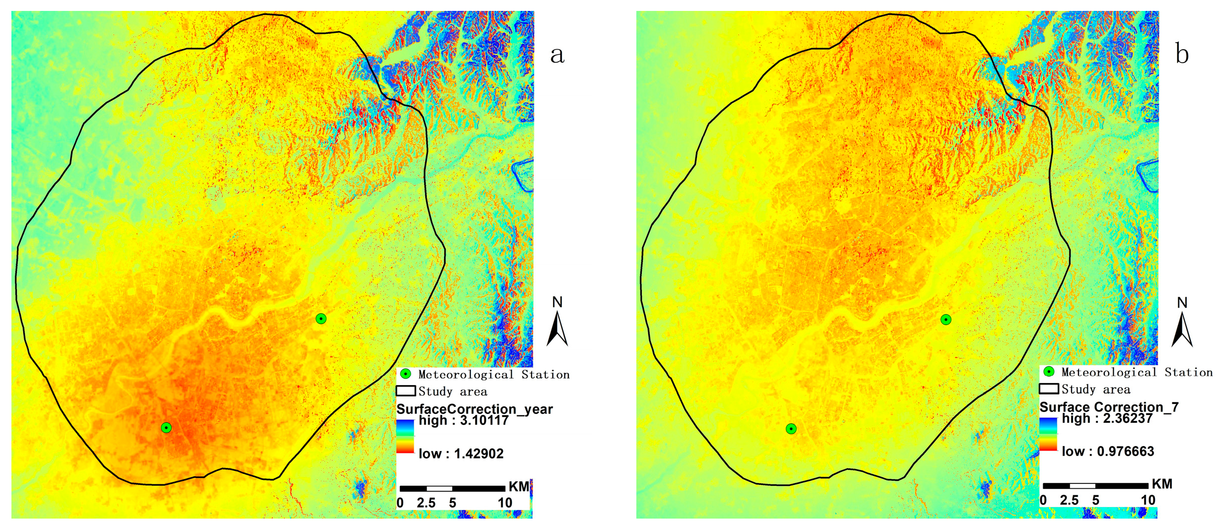
Surface Correction

The average wind speed decreases gradually from the outskirts to the inner ring of the city due to continuous friction and energy consumption by uneven urban buildings [55]. Moreover, numerous studies have established a notable negative correlation between wind speed and the intensity of urban heat islands [55,56,57]. To correct for wind speed, z₀ and LST are employed. Previous research indicates that surface roughness reduces the prevailing wind speeds of urban areas by approximately 20–30% compared to the suburbs [58]. Additionally, studies have shown that urban anemometers record wind speeds that are 10–20% lower than those measured in nearby open areas [59].

$$R_{\mathit{ij}}=\left(A - A_{\mathit{ij}}\right)\times 0.01$$

(5)

where A represents either z₀ or LST at the reference site, A_ij denotes z₀ or LST of cell j after reclassification, and R_ij signifies the correction factor for z₀ or LST relative to the wind speed at the reference point of pixel j. If A_ij > A, the wind speed at pixel j decreases by 1% for each step away from the reference point. Conversely, if A_ij < A, the wind speed increases by 1% for each step away from the reference point. When A_ij = A, the wind speed remains unchanged.

$$R=0.5\times \mathit{\left(}{R}_{z_0}+R_{\mathit{LST}}\mathit{\right)}$$

(6)

$$F_2=F_1+R\times F_A$$

(7)

where R represents the comprehensive correction factor, Rz₀ is the correction factor of z₀, and R_LST is the correction factor of LST, each weighted equally at 0.5. F₂ denotes the wind speed corrected for surface effects, while F₁ represents the wind speed corrected for terrain. F_A is the measured wind speed at the reference point.

2.3.3. Carbon Emission Accounting and Spatialization

Carbon Emission Accounting

Carbon emissions are computed based on land use types, where forest land, grassland, water bodies, and unused land are considered carbon sinks [60], while cultivated land and construction land are identified as carbon sources [61]. The carbon emissions from individual pixels of non-construction land are determined using the direct carbon emission factor method, expressed by the following formula:

$$e_i={\delta }_i\times 900$$

(8)

where e_i represents the carbon emissions attributed to various types of non-construction land, measured in metric tons (t). δ_i (refer to Table S3) denotes the emission coefficients specific to different land classes, expressed in t/m². Each cell has an area of 900 m².

Carbon emissions from construction land are estimated indirectly using carbon emission coefficients associated with various forms of energy consumption. The formula is as follows:

$$\mathit{EC}=\mathit{\sum }e{c}_i=\mathit{\sum }{\mathit{En}}_i{\sigma }_i{\phi }_i$$

(9)

where EC represents the total carbon emissions from construction land, measured in t. ec_i denotes the carbon emissions produced by the combustion of different energy sources. En_i stands for the consumption of different energy sources, measured in t. σ_i represents the standard coal coefficient. φ_i is the carbon emission coefficient. Refer to Table S4 for the specific values of σ_i and φ_i.

Spatialization of Carbon Emissions

Since the study area is not constrained by administrative district boundaries, though the consumption of various types of energy is calculated based on these districts, the total carbon emissions from construction land in Shenyang is initially computed. Subsequently, these emissions are allocated to pixels according to the following steps:

(a)

Based on the intensity of human activities at different POIs, weights are assigned using the analytic hierarchy process (Table S5). The kernel density estimation results of the POIs are then computed to derive the POI energy consumption factor (ECF) based on these weights.

(b)

The road network is categorized into expressways, main roads, secondary roads, and other roads. Weights of 2.39, 1.96, 1.30, and 1.00 are assigned based on the width of each road grade, while railways are weighted at 4.07 [62]. The kernel density estimation of the road traffic ECF is calculated based on assigned weights.

(c)

The energy consumption factors are normalized. Given that POIs encompass carbon emissions from both production activities and daily life, the POI ECF is assigned a weight of two-thirds (2/3), whereas the transportation ECF is given a weight of one-third (1/3). The comprehensive ECF is derived from the weighted sum of these two. A masking process is then employed using the extent of the built-up areas, and the carbon emissions within these zones are spatialized using the following equation:

$${\mathit{EC}}_{\mathrm{i}}=A_i/A\times EC$$

(10)

where EC_i is the carbon emission of pixel i, A_i is the comprehensive ECF of pixel i, A is the sum of the comprehensive ECF of the construction land, and EC signifies the total carbon emissions of the construction land.

2.3.4. Quantify “Instantaneous” ECSS Flow

When horizontal atmospheric movements occur in a region, the CO₂ emissions generated are transported by the atmosphere to distant locations and are absorbed in carbon sink areas along the way [22,63,64]. In regions experiencing persistent and steady winds, accumulated CO₂ is carried away by the atmosphere. Simultaneously, CO₂ emissions continue within the area. Over time, after a period of atmospheric dispersion, the CO₂ concentration in the area stabilizes. This phenomenon can be expressed as follows:

$$C_i{=C}_1{+C}_2$$

(11)

where C_i denotes the amount of CO₂ in a stabilized downwind area i, C₁ represents the CO₂ carried by the wind passing through area i, and C₂ signifies the CO₂ produced by area i itself during the time the wind traverses it.

In this study, inlet vents are strategically located in the northwest, west, and southwest directions. The analysis considers five scenarios where wind diverges towards the downwind direction (Figure 3). Upwind pixels are cut by a wind line passing through the intersection of four pixels, with subsequent airflow dividing and flowing into neighboring pixels that share a common edge. The fraction of CO₂ entering neighboring pixels is determined by the proportion of the area of the upwind pixel following segmentation.

Taking Case 1 as an example, the calculation process is detailed in Equations (S3) and (S4). Beginning from the air inlet, each grid is traversed following the wind direction to estimate the “instantaneous” ECSS flow in the study area. This scenario can be effectively illustrated when the prevailing wind is steady and consistent; the carbon flux within a pixel is included in the amount of CO₂ from the moment the wind enters to just before it leaves.

3. Results

3.1. Simulation of Wind Directions

The high values of z₀ (Figure S2) are predominantly found in construction land, which significantly impedes wind circulation. Conversely, areas with low z₀ values, such as open suburbs, rivers, parks, and green spaces, facilitate wind movement.

The potential ventilation paths for southwest, west, and northwest dominant winds are depicted in Figure 4a1–a3. In suburban areas, where the frictional effects of the underlying surface are minimal, the paths appear relatively straight. However, there are noticeable turns in urban areas.

The prevailing wind directions from the southwest, west, and northwest were determined by interpolating the wind direction points distributed along the potential ventilation pathways (Figure 4b1–b3). The direction of the wind flows follows the trajectory of the respective potential ventilation paths, effectively addressing the westerly wind requirements in the study area and illustrating the impact of urban building distribution on wind patterns. Controlling the orientation of the air inlet allows the simulation of wind flow fields in various scenarios. This paper focuses solely on these three directions as examples.

3.2. Wind Speed Interpolation and Correction

The distribution of the meteorological stations selected for this study is depicted in Figure S3. AAWS (Figure 5a1) and JAWS (Figure 5b1) were interpolated using Kriging methods. The AAWS ranges between 1.89 m/s and 2.34 m/s; thus, it is higher than the JAWS, which ranges from 1.40 m/s to 1.81 m/s. Both datasets indicate lower wind speeds in urban areas and higher speeds in suburban regions. Following correction for slope, aspect, and slope position (Figure 5a2,b2), the overall wind speed trends remained consistent. The AAWS ranged from 1.47 m/s to 2.79 m/s, and JAWS from 1.06 m/s to 2.01 m/s, with the maximum values increasing and the minimum values decreasing compared to the pre-correction levels. The areas exhibiting changes in wind speed are primarily located in the hills on the eastern side of the study area, where topography exerts a significant influence, resulting in noticeable local variations post-correction.

The surface correction results are illustrated in Figure 6, where the AAWS ranges from 1.43 m/s to 3.10 m/s, and the JAWS ranges from 0.98 m/s to 2.37 m/s. For the Shenyang station, the statistically measured AAWS was 2.087 m/s, corrected to 2.192 m/s, resulting in a discrepancy of 0.104 m/s. The JAWS, initially recorded at 1.5 m/s, was adjusted to 1.575 m/s, with an error of 0.075 m/s. For the Shenbei New District station, the measured AAWS was 1.975 m/s, which was later adjusted to 2.108 m/s, showing a discrepancy of 0.133 m/s. The JAWS, originally 1.4 m/s, was corrected to 1.49 m/s, with an error of 0.09 m/s.

The corrected values exhibit relatively minor deviations from the actual measured data; notably, smaller errors were observed for the JAWS compared to the annual averages. In addition, the corrected wind speed presents disparities arising from variations in the terrain and the urban architecture, thereby exhibiting a wealth of detailed information.

3.3. Carbon Emission Accounting and Spatialization

Figure 7a illustrates that areas with elevated values of the comprehensive ECF are clustered concentrations and strip-shaped distributions in the urban center, while the remainder is primarily dispersed along road networks. This spatial pattern is closely tied to the geographical characteristics of the POI and the accessibility provided by the transportation infrastructure. Most POIs typically prioritize factors such as convenient transportation and high pedestrian traffic when selecting locations. Concurrently, some factories, driven by lower land costs or the need to mitigate environmental impacts, choose suburban sites. As a result, sporadic clusters of high-value zones are also observed in the southwestern, western, and northern suburban areas.

The spatial distribution pattern of carbon emissions from the construction land is similar to the comprehensive ECF (Figure 7b), with individual pixels showing that the highest carbon emission reached 534.662 t. The carbon emissions per pixel from the cultivated land, forest land, grassland, water area, and unused land are 0.04473 t, −0.05796 t, −0.00198 t, −0.02277 t, and −0.00045 t, respectively. Carbon sinks serve as the supply areas for ECSS, while carbon sources represent the demand areas. In the study area, the supply areas are small and sparsely distributed and offer limited carbon sequestration capacity per unit area. In contrast, the demand areas, such as urban regions, are larger and have a significantly higher demand for ECSS. Consequently, urban areas alone cannot sufficiently meet their carbon cycling needs.

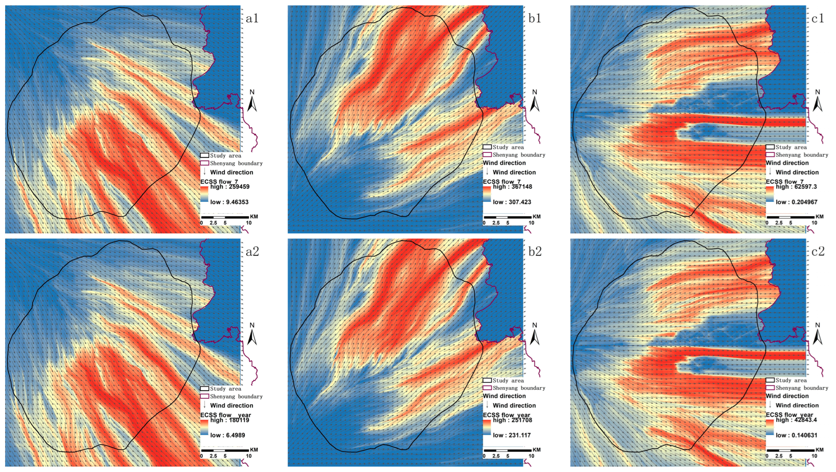
3.4. ECSS Flow

For a single pixel, the carbon flux under JAWS shows distinct ranges: the northwest wind ranges from 0 to 338692 g, the southwest wind from 307.423 to 367148 g, and the west wind from 0.205 to 62,597.3 g. At AAWS, the carbon flux for the northwest wind ranges from 6.499 to 180119 g, for the southwest wind from 231.117 to 251708 g, and for the westerly wind from 0.141 to 42,843.4 g. The intensity of wind speed does not alter the direction of the carbon sequestration service flow. Despite the lower JAWS compared to the AAWS, the paths of the carbon sequestration service flows under the same prevailing wind direction largely overlap, as illustrated in Figure 8a1,a2,b1,b2,c1,c2. However, there are discrepancies in carbon fluxes corresponding to the same pixel, with higher fluxes observed under JAWS compared to AAWS.

Wind direction significantly influences both the direction and flux of ECSS flow, as illustrated in Figure 8a1,a2,b1,b2,c1,c2. The distribution of ECSS flow is not uniform. There exist distinct corridors of ECSS aligned with the prevailing wind direction, varying in width and length. Under stable wind conditions, corridors remain relatively straight, facilitating stable and concentrated flows with higher central fluxes and lower edge fluxes. When wind directions shift, corridors adjust accordingly, potentially causing losses during the accumulation of carbon flux. Forked winds create multiple corridors, and converging winds merge these corridors.

The duration of “instantaneous” ECSS flow varies and is relative; it is determined by the longest path of airflows within a pixel (Figure 4) and the wind speed and is inversely proportional to wind speed and directly proportional to path length. It is also inversely proportional to the rate of air exchange within the cell. For JAWS, the time per single pixel ranges from 14.6 to 42.6 s (Figure 8a3–c3), and for AAWS, it ranges from 10.0 to 28.5 s (Figure 8a4–c4). Spatially, the time consumption patterns of JAWS and AAWS in the same wind direction exhibit similarities.

4. Discussion

4.1. Impact of Air Inlet Position Changes on ECSS Flows

To assess the impact of air inlet position on ECSS flows, the study expanded its scope by adjusting the air inlets for the northwest and southwest winds from air inlet 1 to air inlet 2, with the AAWS. The findings are presented in Figure S4. It is evident that within the original study area, the ECSS flow corridors differ between Figure S4a and Figure 8a2, whereas the results for Figure S4b and Figure 8b2 are remarkably similar. This occurs because, for the northwest wind, air inlet 2 is positioned further westward than northward relative to air inlet 1. Consequently, the air inlet’s position shifts counterclockwise relative to the original study area, causing the direction of the northwest wind in the eastern part of the region to rotate accordingly. The air inlet for the southwest wind not rotated, resulting in no alteration in the shape of the ECSS flow under this prevailing wind direction. This indicates that the orientation of the air inlet relative to the study area is the primary factor influencing the direction of the ECSS flow, while the distance between the air inlet and the study area plays a less significant role.

Additionally, as illustrated in Figure S4, thinner and longer ECSS flow corridors extend beyond the original study area. These corridors originate from significant carbon emission sources, such as small towns or transportation hubs. While these areas differ in shape and size from the urban area of the original study, their ECSS flows can still be effectively captured. Thus, the model presented in this paper is applicable for simulating service flows from carbon emission sources of varying sizes.

4.2. Sustainability of ECSS Supply and Demand

After the ECSS flows stabilize, we calculate the total carbon surplus within the study area for different wind directions and speeds, along with the area of different land types required to sequester this carbon within one year, as detailed in Table S6. Under identical wind speeds, the southwest wind yields the highest total carbon surplus, followed by the northwest wind, with the west wind producing the lowest surplus. This ranking aligns with the lengths of the ECSS flow paths under the three wind directions in the study area (Figure 8a1,b1,c1). The findings suggest that shorter service flow paths facilitate more efficient completion of the ECSS. The prevailing winds in the study area are westerly, suggesting that urban development should primarily focus on the northern and southern sides, with moderate development along the east–west axis. Under the same wind direction, the total carbon surplus at the JAWS exceeds that at the AAWS, as the JAWS is lower than the AAWS. Generally, summer wind speeds are lower and winter wind speeds are higher. Higher wind speeds facilitate more effective completion of the ECSS flow. Therefore, during the summer, it is crucial to enhance carbon control management strategies to mitigate the urban heat island effect.

According to the data in Table S6, even the smallest carbon surplus to be absorbed necessitates approximately 10,600 hectares of forest land over the course of a year. Larger areas are required for grasslands, water bodies, and unused land. These data represent the carbon surplus at a single point in time, but carbon emissions and sequestration are continuous processes. Over the course of a year, the cumulative total carbon surplus in the study area is approximately 16.7018 million tons, necessitating roughly 25.9345 million hectares of forest land to fully absorb this carbon. This area is equivalent to about 136 times the size of Changbai Mountain National Forest Park, whereas the study area itself covers only 132,400 hectares. This indicates that a moderately developed urban area would require forest land approximately ten times its own size to provide adequate ECSS. In reality, the limited availability of carbon sink areas relative to the numerous cities creates a mismatch between demand and supply, potentially compromising the sustainability of ES.

4.3. Evaluation of the Method and Limitations of Its Application

ECSS is a crucial ecosystem service with significant implications for environmental sustainability and human well-being. Understanding the spatial patterns of ECSS flows is essential for assessing the current state of the carbon cycle. Atmospheric circulation operates on a global scale; thus, the effectiveness of ECSS should be considered on a global scale as well. Our research addresses only a specific segment of it. CO₂ moves from the demand area to the supply area, and once CO₂ exits the demand area, the ECSS can be considered to be complete at that end. This study simulates the ECSS flow in the Shenyang urban area by precisely quantifying the wind environment. It analyzes the flow characteristics, explores the spatial distribution law of CO₂, and offers recommendations for balancing the supply and demand of urban ECSS, as well as for the scientific management of CO₂.

The wind environment simulated in this study includes prevailing wind direction and wind speed. The orientation and distance of the inlet for the prevailing wind can be adjusted based on the wind frequency in the study area, allowing the simulation of wind from any direction. This approach also avoids issues such as low interpolation accuracy of wind direction due to the scattered distribution of meteorological data. After calibration, the simulated wind speed shows minimal error when compared to the statistical data from meteorological stations and effectively captures variations in wind speed resulting from surface morphology. The wind environment simulated using this method offers high spatial resolution, is cost-effective, and relies on readily accessible data. Additionally, the model is simple to implement and well suited for small-scale regional studies. However, the method has certain limitations. It can simulate only one wind direction at a time and does not reflect dynamic changes in wind direction at a given location. Therefore, enhancements are needed to enable the model to simulate temporal variations in wind direction. Similarly, while the average wind speed can capture seasonal variations, it does not reflect real-time changes in wind speed.

ECSS flows are categorized into latent flows and actual flows [65,66]. The ECSS flows simulated in this study fall under latent flows, representing a virtual process with potential spatial and temporal movement trends following the dominant wind direction [67,68]. Given the limitations of wind environment simulation, we are only able to model the ECSS flow under a specific prevailing wind direction, without capturing the dynamic processes of flow direction and velocity. Additionally, the carbon emission rate used in the simulation is based on an average value rather than direct measurements. Furthermore, our calculations were simplified by assuming the presence of a boundary upwind of the air inlet but not downwind. This assumption implies that CO₂ levels outside the air inlet do not affect the study area, while CO₂ from the study area can influence regions beyond the downwind boundary. This paper visualizes the ECSS flow under the prevailing wind direction using a carbon flux grid. The results reflect the fact that the carbon sequestration services in the study area are in a state of demand falling short of supply. The identified ECSS flow corridors can provide a foundation for planning construction and ecological protection efforts.

4.4. Policy Recommendations

Based on the ECSS flow results for the three prevailing wind directions, three levels of corridors were identified (Figure S5). As the corridor level increases, the carbon flow per unit area decreases, while the corridor’s importance grows. To mitigate pressure on the first-level corridors, it is recommended to enhance ecological restoration and construction within the second- and third-level corridors, intercepting CO₂ upstream as much as possible. In urban areas upstream of these corridors, space can be efficiently utilized for the construction of small wetlands or pocket parks. Additionally, efforts should be intensified to improve the ecological management of rivers and lakes, as water bodies possess a carbon sink capacity second only to forests. Downstream, near hilly areas, strategies such as reforestation and grassland restoration should be implemented. Along the corridors, linear green spaces, such as wedge-shaped greenspaces and green corridors, should be established; buildings within these areas should only be low-rise types, and they should be less dense to minimize wind resistance, thereby facilitating the smooth exit of CO₂ from the urban areas [69].

Most importantly, implementing robust measures to control carbon emissions and reduce the demand for ECSS is crucial, as this will yield positive effects across economic, social, and environmental dimensions. The rise in carbon emissions has contributed to global warming, highlighting a global deficit in ECSS. Effective strategies to manage carbon emissions include improving energy efficiency, optimizing energy structures, and implementing carbon trading systems. Additionally, advancing low-carbon technologies to capture carbon at emission sources or downstream of carbon sequestration corridors, followed by storage or utilization, is essential. Building green ecological cities and reducing urban carbon emissions can help mitigate the imbalance between the supply and demand for ECSS, thus supporting the sustainability of ES.

5. Conclusions

The results indicate the following: (1) The simulated dominant wind direction aligns closely with the trend of the potential ventilation pathways. The error between the post-corrected wind speeds and statistical data from two meteorological stations in the calibrated area is minimal, highlighting the differences in wind speed caused by various terrain conditions and building forms. (2) The study area experiences significant carbon emissions, with peak concentrations concentrated in the urban center and the remainder of the emissions dispersed across the road network in peripheral areas. There is a notable demand for ECSS within this region. (3) The direction of ECSS flow is determined by the prevailing wind direction, with wind speed influencing the flow velocity. The flow volume displays spatial heterogeneity across the region. The time consumption of a single pixel in the ECSS flow is influenced by both wind speed and the airflow path, reflecting the exchange rate of airflows within the cell. (4) The study area experiences a significant carbon surplus, resulting in a mismatch between the supply of ECSS and the growing demand. This imbalance poses challenges to the sustainable development of urban areas and the provision of ES. To address these issues, it is crucial to implement thoughtful urban planning and renovation strategies aimed at improving the efficiency of ECSS flows. Additionally, enhanced carbon management is necessary to sustainability.

References

- Costanza, R.; d’Arge, R.; Groot, R.d.; Farber, S.; Grasso, M.; Hannon, B.; Limburg, K.; Naeem, S.; O’Neill, R.; Paruelo, J.; et al. The value of the world’s ecosystem services and natural capital. Ecol. Econ. 1998, 25, 3–15. [Google Scholar] [CrossRef]
- Tao, Y.; Tao, Q.; Sun, X.; Qiu, J.X.; Pueppke, S.G.; Ou, W.X.; Guo, J.; Qi, J.G. Mapping ecosystem service supply and demand dynamics under rapid urban expansion: A case study in the Yangtze River Delta of China. Ecosyst. Serv. 2022, 56, 101448. [Google Scholar] [CrossRef]
- Bryan, B.A.; Ye, Y.; Zhang, J.; Connor, J.D. Land-use change impacts on ecosystem services value: Incorporating the scarcity effects of supply and demand dynamics. Ecosyst. Serv. 2018, 32, 144–157. [Google Scholar] [CrossRef]
- Fisher, B.; Turner, R.K.; Morling, P. Defining and classifying ecosystem services for decision making. Ecol. Econ. 2009, 68, 643–653. [Google Scholar] [CrossRef]
- Jones, L.; Norton, L.; Austin, Z.; Browne, A.L.; Donovan, D.; Emmett, B.A.; Grabowski, Z.J.; Howard, D.C.; Jones, J.P.G.; Kenter, J.O. Stocks and flows of natural and human-derived capital in ecosystem services. Land Use Policy 2016, 52, 151–162. [Google Scholar] [CrossRef]
- Liu, H.; Liu, L.; Ren, J.; Bian, Z.; Ding, S. Progress of quantitative analysis of ecosystem service flow. Chin. J. Appl. Ecol. 2017, 28, 2723–2730. [Google Scholar]
- Schirpke, U.; Candiago, S.; Vigl, L.E.; Jäger, H.; Labadini, A.; Marsoner, T.; Meisch, C.; Tasser, E.; Tappeiner, U. Integrating supply, flow and demand to enhance the understanding of interactions among multiple ecosystem services. Sci. Total Environ. 2019, 651, 928–941. [Google Scholar] [CrossRef]
- Ecosystems and Human Well-Being: Synthesis. Available online: https://www.millenniumassessment.org/documents/document.356.aspx.pdf (accessed on 20 April 2024).
- Zang, Z.; Zou, X.-Q. Connotation characterization and evaluation of ecological well-being based on ecosystem service theory. Chin. J. Appl. Ecol. 2016, 27, 1085–1094. [Google Scholar]
- Wang, Z.; Zhang, L.; Li, X.; Li, Y.; Frans, V.F.; Yan, J. A network perspective for mapping freshwater service flows at the watershed scale. Ecosyst. Serv. 2020, 45, 101129. [Google Scholar] [CrossRef]
- Gao, X.; Huang, B.; Hou, Y.; Xu, W.; Zheng, H.; Ma, D.; Ouyang, Z. Using ecosystem service flows to inform ecological compensation: Theory & application. Int. J. Environ. Res. Public Health 2020, 17, 3340. [Google Scholar] [CrossRef]
- Zhao, Y.; Wu, F.; Li, F.; Chen, X.; Xu, X.; Shao, Z. Ecological compensation standard of trans-boundary river basin based on ecological spillover value: A case study for the Lancang–Mekong River Basin. Water 2021, 18, 1251. [Google Scholar] [CrossRef] [PubMed]
- Su, K.; Sun, X.; Guo, H.; Long, Q.; Li, S.; Mao, X.; Niu, T.; Yu, Q.; Wang, Y.; Yue, D. The establishment of a cross-regional differentiated ecological compensation scheme based on the benefit areas and benefit levels of sand-stabilization ecosystem service. Int. J. Environ. Res. Public Health 2020, 270, 122490. [Google Scholar] [CrossRef]
- Wang, T.; Piao, S. Estimate of terrestrial carbon balance over the Tibetan Plateau: Progresses, challenges and perspectives. Quat. Sci. 2023, 43, 313–323. [Google Scholar]
- Li, T.; Li, J.; Wang, Y. Carbon sequestration service flow in the Guanzhong-Tianshui economic region of China: How it flows, what drives it, and where could be optimized? Ecol. Indic. 2019, 96, 548–558. [Google Scholar] [CrossRef]
- Wu, J.; Fan, X.; Li, K.; Wu, Y. Assessment of ecosystem service flow and optimization of spatial pattern of supply and demand matching in Pearl River Delta, China. Ecol. Indic. 2023, 153, 110452. [Google Scholar] [CrossRef]
- Liang, J.; Pan, J. Identifying carbon sequestration’s priority supply areas from the standpoint of ecosystem service flow: A case study for Northwestern China’s Shiyang River Basin. Sci. Total Environ. 2024, 927, 172283. [Google Scholar] [CrossRef]
- Xu, Z.; Wei, H.; Fan, W.; Wang, X.; Zhang, P.; Ren, J.; Lu, N.; Gao, Z.; Dong, X.; Kong, W. Relationships between ecosystem services and human well-being changes based on carbon flow—A case study of the Manas River Basin, Xinjiang, China. Ecosyst. Serv. 2019, 37, 100934. [Google Scholar] [CrossRef]
- Yang, J.; Li, J.; Guan, X. Spatio-Temporal Pattern and Driving Mechanism of Ecosystem Carbon Sequestration Services in the Wujiang River Basin. Res. Environ. Sci. Res. Environ. Sci. 2023, 36, 757–767. [Google Scholar]
- Hong, W.; Bao, G.; Du, Y.; Guo, Y.; Wang, C.; Wang, G.; Ren, Z. Spatiotemporal changes in supply–demand patterns of carbon sequestration services in an urban agglomeration under China’s rapid urbanization. Remote Sens. 2023, 15, 811. [Google Scholar] [CrossRef]
- Wu, C.; Lu, R.; Zhang, P.; Dai, E. Multilevel ecological compensation policy design based on ecosystem service flow: A case study of carbon sequestration services in the Qinghai-Tibet Plateau. Sci. Total Environ. 2024, 921, 171093. [Google Scholar] [CrossRef]
- Wang, Q.; Liu, S.; Wang, F.; Liu, H.; Liu, Y.; Yu, L.; Sun, J.; Tran, L.-S.P.; Dong, Y. Quantifying carbon sequestration service flow associated with human activities based on network model on the Qinghai-Tibetan. Front. Environ. Sci. 2022, 10, 900908. [Google Scholar] [CrossRef]
- Liu, W.; Zhan, J.; Zhao, F.; Zhang, F.; Teng, Y.; Wang, C.; Chu, X.; Kumi, M.A. The tradeoffs between food supply and demand from the perspective of ecosystem service flows: A case study in the Pearl River Delta, China. J. Environ. Manag. 2022, 301, 113814. [Google Scholar] [CrossRef] [PubMed]
- Zhai, T.; Wang, J.; Fang, Y.; Huang, L.; Liu, J.; Zhao, C. Integrating ecosystem services supply, demand and flow in ecological compensation: A case study of carbon sequestration services. Sustainability 2021, 13, 1668. [Google Scholar] [CrossRef]
- Qin, K.; Liu, J.; Yan, L.; Huang, H. Integrating ecosystem services flows into water security simulations in water scarce areas: Present and future. Sci. Total Environ. 2019, 670, 1037–1048. [Google Scholar] [CrossRef]
- Bagstad, K.J.; Villa, F.; Batker, D.; Harrison-Cox, J.; Voigt, B.; Johnson, G.W. From theoretical to actual ecosystem services: Mapping beneficiaries and spatial flows in ecosystem service assessments. Ecol. Soc. 2014, 19, 64. [Google Scholar] [CrossRef]
- Guo, F.; Zhang, H.; Fan, Y.; Zhu, P.; Wang, S.; Lu, X.; Jin, Y. Detection and evaluation of a ventilation path in a mountainous city for a sea breeze: The case of Dalian. Build. Environ. 2018, 145, 177–195. [Google Scholar] [CrossRef]
- He, Y.; Liu, Z.; Ng, E. Parametrization of irregularity of urban morphologies for designing better pedestrian wind environment in high-density cities–A wind tunnel study. Build. Environ. 2022, 226, 109692. [Google Scholar] [CrossRef]
- Chen, L.; Lu, J.; Yu, W. A quantitative method to detect the ventilation paths in a mountainous urban city for urban planning: A case study in Guizhou, China. Indoor Built Environ. 2017, 26, 422–437. [Google Scholar] [CrossRef]
- Xu, Y.; Wang, W.; Chen, B.; Chang, M.; Wang, X. Identification of ventilation corridors using backward trajectory simulations in Beijing. Sustain. Cities Soc. 2021, 70, 102889. [Google Scholar] [CrossRef]
- Xu, Y.; Wan, X.; Fu, C.; Liu, C. Study of wind speed interpolation in complex terrain—A case of Jilin Province. Front. Earth Sci. 2012, 24, 78–81. [Google Scholar]
- Qi, Y. Vector interpolation of wind fields over complex terrain. Radialization Prot. 2001, 21, 213–218. [Google Scholar]
- Shi, T.; Yan, Y.; Wang, L.; Wang, Z. Large − Scale Wind Speed Simulation Based on DEM. Geogr. Geo-Inf. Sci. 2007, 23, 26–29. [Google Scholar]
- Amaral, S.; Câmara, G.; Monteiro, A.M.V.; Quintanilha, J.A.; Elvidge, C.D. Estimating population and energy consumption in Brazilian Amazonia using DMSP night-time satellite data. Comput. Environ. Urban Syst. 2005, 29, 179–195. [Google Scholar] [CrossRef]
- Elvidge, C.D.; Baugh, K.E.; Kihn, E.A.; Kroehl, H.W.; Davis, E.R.; Davis, C.W. Relation between satellite observed visible-near infrared emissions, population, economic activity and electric power consumption. J. Remote Sens. 1997, 18, 1373–1379. [Google Scholar] [CrossRef]
- Wu, J.; Niu, Y.; Peng, J.; Wang, Z.; Huang, X. Research on energy consumption dynamic among prefecture-level cities in China based on DMSP/OLS Nighttime Light. Geographical Research. Geogr. Res. 2014, 33, 625–634. [Google Scholar]
- Zhang, X.; Zhao, T.; Xu, H.; Liu, W.; Wang, J.; Chen, X.; Liu, L. GLC_FCS30D: The first global 30 m land-cover dynamic monitoring product with a fine classification system for the period from 1985 to 2022 generated using densetime-series Landsat imagery and the continuous change-detection method. Earth Syst. Sci. Data 2024, 16, 1353–1381. [Google Scholar] [CrossRef]
- Wu, W.-B.; Ma, J.; Banzhaf, E.; Meadows, M.E.; Yu, Z.-W.; Guo, F.-X.; Sengupta, D.; Cai, X.-X.; Zhao, B. A first Chinese building height estimate at 10 m resolution (CNBH-10 m) using multi-source earth observations and machine learning. Remote Sens. Environ. 2023, 291, 113578. [Google Scholar] [CrossRef]
- Jiang, X.; Ming, X.; Zhang, J.; Zhang, S.; Zhang, S. Distribution Characteristics and Exploitation and Utilization of Wind Energy Resources of Shenyang City, China. Resour. Sci. 2009, 31, 1764–1771. [Google Scholar]
- Gong, Q.; Wang, H.; Zhu, L.; Lin, N.; Gu, Z.; Chao, H.; Xu, H. Study on the Near SurfaceWind Shear Characteristics in Liaoning Province. J. Nat. Resour. 2015, 30, 1560–1569. [Google Scholar]
- Mihailović, D.; Lalić, B.; Rajković, B.; Arsenić, I. A roughness sublayer wind profile above a non-uniform surface. Bound. -Layer Meteorol. 1999, 93, 425–451. [Google Scholar] [CrossRef]
- Yue, T.; Wang, W.; Yu, Q.; Zhu, Z.; Zhang, S.; Zhang, R.; Du, P. Simulation of Vertical Wind Profile and Its Relevant Parameters under Neutral Condition. Resour. Sci. 2006, 28, 136–144. [Google Scholar]
- Zhang, Y.; Shen, X. Simulation Analysis of Vegetation Covered Surface’s Aerodynamics Roughness Length and Zero Displacement. J. Desert Res. 2008, 28, 21–26. [Google Scholar]
- Li, J.; You, S.; Huang, J. Spatial distribution of ground roughness length based on GIS in China. J. Shanghai Jiaotong Univ. (Agric. Sci.) 2006, 24, 185–189. (In Chinese) [Google Scholar]
- Li, Q.; Cai, X.; Song, Y. Research of the distribution of national scale surface roughness length with high resolution in China. Plateau Meteorol. 2014, 33, 474–482. [Google Scholar]
- Kang, L.; Yang, Z.; Zhang, J.; Zou, X.; Wen, Z. Wind tunnel simulation for comparison of wind velocity profile characteristics at two flexible plant surfaces. J. Desert Res. 2020, 40, 43. [Google Scholar]
- Jasinski, M.F.; Crago, R.D. Estimation of vegetation aerodynamic roughness of natural regions using frontal area density determined from satellite imagery. Agric. For. Meteorol. 1999, 94, 65–77. [Google Scholar] [CrossRef]
- Garratt, J.R. The atmospheric boundary layer. Earth-Sci. Rev. 1994, 37, 89–134. [Google Scholar] [CrossRef]
- Burian, S.; Brown, M.; Augustus, N. Development and assessment of the second generation National Building Statistics database. In Proceedings of the Seventh Symposium on the Urban Environment, San Diego, CA, USA, 11 September 2007. [Google Scholar]
- Yue, T.X.; Wang, W.; Yu, Q.; Zhu, Z.; Zhang, S.H.; Zhang, R.H.; Du, Z. Simulation of vertical wind profile under neutral conditions. International J. Remote Sens. 2007, 28, 2207–2219. [Google Scholar] [CrossRef]
- Lettau, H. Note on aerodynamic roughness-parameter estimation on the basis of roughness-element description. J. Appl. Meteorol. 1969, 8, 828–832. [Google Scholar] [CrossRef]
- Qiao, Z.; Xu, X.; Wu, F.; Luo, W.; Wang, F.; Liu, L.; Sun, Z. Urban ventilation network model: A case study of the core zone of capital function in Beijing metropolitan area. J. Clean. Prod. 2017, 168, 526–535. [Google Scholar] [CrossRef]
- Shen, X.; Zhao, R.; He, R.; Wang, Q.; Guo, Y. Research on Urban Wind Environment Simulation: A Case Study of Zhengzhou Central Area. J. Geo-Inf. Sci. 2020, 22, 1349–1357. [Google Scholar]
- Wong, M.S.; Nichol, J.E.; To, P.H.; Wang, J. A simple method for designation of urban ventilation corridors and its application to urban heat island analysis. Build. Environ. 2010, 45, 1880–1889. [Google Scholar] [CrossRef]
- Xu, W.; Zhang, L.; Qi, L.; Liu, D.; Zhang, S.; Cao, D. Observation Analysis of the Influence of Surface Wind on Urban Heat Island in Shanghai. Meteorological Monthly J. Appl. Meteorol. Climatol. 2019, 45, 1262–1277. [Google Scholar]
- Huang, Q.; Lu, Y. Long-term Trend of Urban Heat Island Intensity and Climatological Affecting Mechanism in Bejing City. Sci. Geogr. Sin. 2018, 38, 1715–1723. [Google Scholar]
- Alonso, M.; Fidalgo, M.; Labajo, J.L. The urban heat island in Salamanca (Spain) and its relationship to meteorological parameters. Clim. Res. 2007, 34, 39–46. [Google Scholar] [CrossRef]
- Zhou, S.; Shu, J. Urban Climatology; Meteorological Press: Beijing, China, 1994; ISBN 7–5029–1645–8. [Google Scholar]
- Bornstein, R. Observed urban-rural wind speed differences in New York City. In Proceedings of the AGU National Fall Meeting, San Francisco, CA, USA, 15–18 December 1969. [Google Scholar]
- Ma, X.; Wang, Z. Progress in the study on the impact of land-use change on regional carbon sources and sinks. Acta Ecol. Sin. 2015, 35, 5898–5907. [Google Scholar]
- Sun, X. Effects of carbon emission by land use patterns in Hefei’s economic circle of Anhui province. Resour. Ecol. 2012, 27, 394–401. [Google Scholar]
- Fu, B.; Zhai, J.; Xu, Y.; Zhao, B.; Xie, X.; Xue, B. Mapping urban-rural energy consumption pattern based on the POl data: A case study of Weifang City, Shandong Province. J. Earth Environ. 2023, 14, 774–785. [Google Scholar] [CrossRef]
- Janzen, H. Carbon cycling in earth systems—a soil science perspective. Agric. Ecosyst. Environ. 2004, 104, 399–417. [Google Scholar] [CrossRef]
- The Carbon Cycle and Atmospheric Carbon Dioxide. Available online: https://hal.science/hal-03333974/document (accessed on 3 September 2021).
- Cortinovis, C.; Geneletti, D. A framework to explore the effects of urban planning decisions on regulating ecosystem services in cities. Ecosyst. Serv. 2019, 38, 100946. [Google Scholar] [CrossRef]
- Lourdes, K.T.; Hamel, P.; Gibbins, C.N.; Sanusi, R.; Azhar, B.; Lechner, A.M. Planning for green infrastructure using multiple urban ecosystem service models and multicriteria analysis. Landsc. Urban Plan. 2022, 226, 104500. [Google Scholar] [CrossRef]
- Syrbe, R.-U.; Walz, U. Spatial indicators for the assessment of ecosystem services: Providing, benefiting and connecting areas and landscape metrics. Ecol. Indic. 2012, 21, 80–88. [Google Scholar] [CrossRef]
- Pulselli, F.M.; Coscieme, L.; Bastianoni, S. Ecosystem services as a counterpart of emergy flows to ecosystems. Ecol. Model. 2011, 222, 2924–2928. [Google Scholar] [CrossRef]
- Ren, C.; Yuan, C.; Ho, C.K.; Ng, Y.Y. A Study of Air Path and Its Application in Urban Planning. Urban Plan. Forum 2014, 3, 52–60. (In Chinese) [Google Scholar]
Disclaimer/Publisher’s Note: The statements, opinions and data contained in all publications are solely those of the individual author(s) and contributor(s) and not of MDPI and/or the editor(s). MDPI and/or the editor(s) disclaim responsibility for any injury to people or property resulting from any ideas, methods, instructions or products referred to in the content. |
© 2024 by the authors. Licensee MDPI, Basel, Switzerland. This article is an open access article distributed under the terms and conditions of the Creative Commons Attribution (CC BY) license (https://creativecommons.org/licenses/by/4.0/).
Share and Cite
Ma, Y.; Tian, S. Simulation of Urban Carbon Sequestration Service Flows and the Sustainability of Service Supply and Demand. Sustainability 2024, 16, 7738. https://doi.org/10.3390/su16177738
Ma Y, Tian S. Simulation of Urban Carbon Sequestration Service Flows and the Sustainability of Service Supply and Demand. Sustainability. 2024; 16(17):7738. https://doi.org/10.3390/su16177738
Chicago/Turabian StyleMa, Yaoxi, and Shufang Tian. 2024. "Simulation of Urban Carbon Sequestration Service Flows and the Sustainability of Service Supply and Demand" Sustainability 16, no. 17: 7738. https://doi.org/10.3390/su16177738
APA StyleMa, Y., & Tian, S. (2024). Simulation of Urban Carbon Sequestration Service Flows and the Sustainability of Service Supply and Demand. Sustainability, 16(17), 7738. https://doi.org/10.3390/su16177738