Abstract
As firms and consumers engage with environmental issues, decisions for inventory control need to entail this perspective of sustainability. Most green inventory models employ methods such as carbon caps or taxes for dealing with environmental sustainability. This problem can be more generally tackled via an explicit estimation of the environmental drivers of maintaining inventory in a warehouse, paired with the economic perspective within a transparent multi-objective optimization framework. With this goal, this paper builds on a detailed estimation of environmental and cost factors for a continuous-review inventory policy. The bi-objective problem is tackled by keeping the objective functions separate. In particular, the modeling of greenhouse gas emission or cost performance factors for the inventory encompasses factors that can depend on the decision variables, taking into account aspects such as warehouse location, building characterization, energy usage, and transport requirements. The effects of the emission drivers on the multi-objective optimization decisions are analyzed, considering that the problem can be constrained by multiple service level measures. Stockout response can be multifaceted and different service level measures capture different aspects of inventory shortages, affecting the resulting efficient solutions differently. The results highlight the impact of aspects such as warehouse location and supply capacity on solutions for the multi-objective inventory problem. Managerial decisions are thus influenced by warehousing and supply attributes via a traceable link to specific cost and emission determinants.
1. Introduction
The escalating focus on environmental concerns by businesses aiming to mitigate pollution from their operations is being driven by both external pressures from regulations and customer expectations [1]. This challenge is key also in inventory control, as it is one of the crucial components of supply chain management. Road transport is one of the top contributors to carbon emissions [2]. Additionally, product storage and warehousing activities are relevant contributors to inventory emissions, as replenishment frequency and the amount of products in an inventory impact environmental sustainability [3]. In response to this, decarbonization efforts need to be addressed also at the inventory control level, thus moving towards environmentally sustainable inventory systems [4].
Inventory models have been adapted to aspects such as stockouts [5] and service levels [6], and concepts of green supply chains started to appear in the late 1990s [7]. In regard to green inventory management, improving environmental performance of inventories can lead to more robust operations and towards sustainable businesses [8]. In particular, sustainability perspectives other than economic are usually modeled as constraints or additional cost factors [9]. Environmental emissions can be driven by trans-shipment [3], but also by inventory holding due to energy requirements [10]. Moreover, emissions are influenced by order quantities [10], meaning that the understanding of how inventory decisions affects costs and emissions is necessary for sustainable development [11]. Whereas various attempts have been undertaken to incorporate environmental considerations into inventory control models, a comprehensive examination specifically addressing the estimation of the performance factors for storage and reordering is lacking.
With the aim of optimizing the inventory from the different sustainability perspectives of costs and carbon emissions, this work addresses an inventory control approach based on the explicit estimation of the environmental and cost drivers inherent in maintaining inventory within a warehouse. The objective is to improve inventory sustainability by directly relating inventory decisions to sustainability drivers for both the considered perspectives, allowing for greater transparency of the major causes of costs and emissions sustained in order to maintain the inventory of a product. As modern technologies enable continuous review and reordering of inventories [11], we assume that the inventory level is continuously reviewed and procurement operates under a fixed-order resupply policy. More specifically, to fill the gap between performance factor estimation and policies for inventories, this study is dedicated to integrating a comprehensive view of contributors to costs and carbon emissions. This estimation is integrated within a stochastic reorder-level policy, with the aim of optimizing both the economic and the environmental perspectives through a transparent multi-objective optimization framework. Moreover, since different service level measures employed in partial costing inventory models control the shortage events in different ways [12], the problem is constrained by multiple service level functions. Both transport and inventory storage components have an effect on carbon emissions, due to the interplay of system characteristics on different cost and emission aspects. The proposed model supports sustainability of businesses by evaluating and reducing carbon emissions related to inventory management.
The remaining sections of this paper are organized based on the followed research process. After analyzing the relevant literature in Section 2, which allowed us to identify the context of the study and the literature gap, Section 3 describes the inventory problem by defining the objective functions and the related constraints. The problem was developed based on the rationale highlighted by the literature for sustainable inventory control, which requires knowledge of the impact of inventory control decisions on different sustainability aspects, which still lacks integration in quantitative and holistic models. In this regard, Section 4 is devoted to presenting the identification and related modeling of the inventory performance factors from both cost and emission perspectives, which follows the relevant drivers responsible for inventory control efficiency. Section 5 employs a multi-objective optimization procedure for solving the presented problem for a case study application, and quantitative results for a representative case study are explored by comparing different scenarios. The Conclusions, in Section 6, provide a summary of the paper’s key contributions and delve into potential future research directions.
2. Literature Review
The goals of inventory control can be generally described as (i) provide products to consumers, and (ii) provide them in a sustainable way for businesses. The former objective is closely related to product availability, which has been historically supported by aspects such as safety stock for avoiding inventory shortages [13]. Moreover, business sustainability entails not only economic aspects, but also environmental sustainability [9]. This section focuses on literature relevant to these two aspects, with a particular focus on continuous-review inventory policies, as they still appear to be largely tackled with deterministic approaches when considering environmental sustainability [11,14]. Continuous-review models have been the most studied policy considering green aspects [9], and they have the objective to minimize long-run costs by finding optimal control policies [15]. Please refer to the studies of Salas-Navarro et al. [8] and Žic et al. [11] for more details on sustainable inventory models.
One of the approaches to deal with shortages is considering an additional cost component, which stems from economic order quantity generalization of planned shortages [16,17]. However, when demand is stochastic, shortage events become more complex and random [12]. Considering customer service levels is a method to control shortages by the use service level measures, which constrain inventory decisions [6]. Metrics related to these product availability aspects have been developed for different inventory problems. For example, the measure of portion of demand met from the available inventory has been used by Tao et al. [18] within a reorder-level inventory policy, while Bijvank and Vis [19] implemented it for a base-stock policy. More recently, Escalona et al. [12] considered it for a reorder-level policy, and showed how different measures, which are based on different shortage perspectives, affect aspects other than those they directly control. For example, their results highlighted how controlling shortage frequency also affects the fraction of demand that can be met from on-hand inventory. Additionally, service level performance is linked to inventory costs [12].
Papers that deal with integrating environmental sustainability perspectives in the lot-sizing problem mainly consider transport emissions (e.g., [4,20]). When the holding aspect is also considered, the focus is put on operational energy usage, which depends on the storage space occupied by inventory (e.g., [21,22]). Buildings also use energy for both heating and cooling in operations; this depends on the thermal characterization of the building elements [23]. Such models are mostly based around carbon costs, meaning that an economic cost is associated with greenhouse gas emissions, thus contributing to the overall total inventory cost objective function. For example, Utama et al. [3], Kazemi et al. [21] extended the economic order quantity model with additional cost factors that promote sustainability. A similar approach has been followed by Kwak [10] for a periodic policy. Cost-based approaches to environmental sustainability are valuable in the presence of carbon tax regulations [24,25,26]. Another stream of the inventory management literature concentrates instead on explicit environmental modeling along with the classical economic perspective. Underlining the importance of limiting carbon emissions, Hovelaque and Bironneau [27] modeled a separate objective function for environmental sustainability following the deterministic order quantity formulation. Similarly, the works of Bouchery et al. [28], Bozorgi et al. [29] identified an efficient frontier for the deterministic multi-objective inventory problem. While these models better consider this multifaceted sustainability problem by formulating emissions as a primary objective, there seems to be a lack of contributions that extend these works with aspects such as stochasticity of demand or service level constraints. In this direction, Žic and Žic [30] use a weighted approach for solving the multi-objective problem where the emission driver is caused by product transportation, while Pilati et al. [31] developed a transparent bi-objective reorder-level policy formulation which considers costs and emissions due to product waste. These contributions share a common limitation: they do not examine the factors influencing the cost and emission components, and instead they treat carbon emission indices as predetermined. Table 1 highlights this factor, and the fact that most green inventory policies do not include customer service level aspects, for example, via constraints. When emission factors are estimated, the focus is mainly on the trans-shipment driver and the driver categories are not thoroughly analyzed. This analysis backs up the findings of Žic et al. [11], who found that streamlined methods for estimating inventory-related emission are still missing. Moreover, Table 1 highlights the need to extend the previous literature based on deterministic approaches such as the economic order/production quantity to consider more realistic aspects such as customer behavior to stockouts and service level measures. Inventory control can promote green operations primarily by evaluating the impact of decision variables on environmental metrics, transforming the reordering policy objective from merely cost minimization into a multifaceted sustainability challenge. Moreover, it has been shown that measures of service level act on different inventory availability aspects, but no study has included multiple perspectives concurrently.

Table 1.
Comparison between existing and proposed sustainable inventory control models.
3. Problem Definition and Inventory Model Formulation
This study focuses on the optimization of the inventory management for a product via a green continuous-review reorder-level policy, with the goal of optimizing both economic and environmental performance. Specifically, the aim is to identify efficient solutions for the presented inventory problem, where both sustainability perspectives are modeled as primary objective functions. The inventory model is supported by a detailed formulation of both cost and carbon emission factors related to the main inventory determinants of resupply and storage. This emphasizes how inventory managerial decisions are influenced not only by demand attributes, but also by warehousing and supply characteristics via a traceable link to specific cost and emission determinants. In particular, the driver categories for order issue and transport are considered for resupply, while for storage the main categories are related to operational and installation costs or emissions. Section 4 is aimed at presenting the proposed formulation for the estimation of these performance factors.
The considered inventory model is an policy, where a reorder of fixed size Q is issued whenever the inventory level reaches the reorder point r. Demand during the lead time is modeled as a continuous probability density function that can entail both variation in demand itself, or in the lead time duration. In addition, the considered problem tackles inventory shortages via a partial costing formulation with service level constraints. Due to the duality of both economic and environmental objectives, a multi-objective problem needs to be tackled, shifting the optimization goal from sole economic optimality to the identification of efficient solutions. More specifically, an efficient solution for the reorder-level policy is an pair that performs better than any other feasible pair in at least one objective. This approach facilitates the exploration of trade-offs resulting from shifts between efficient solutions, offering decision makers a comprehensive understanding of the impact of inventory decisions on the considered objective functions. The goal is to provide the possible efficient feasible solutions to the decision maker, where feasibility is given by the constrained portion of the problem due to service levels.
The bi-objective optimization problem for the proposed green reorder-level policy is
where and are the economic and environmental objective functions, respectively, and is the vector of service level constraint functions that need to satisfy the related service levels . Both the objective function components and the related performance factors are dependent on the decision variables r and Q, and on inventory system characteristics. Indeed, as better presented in detail in Section 4, inventory performance factors are functions of warehouse and supply characteristics in addition to the decision variables.
Regarding the objective functions, total costs depend on the frequency of reorder and stock held at the inventory. In particular, a variable cost is incurred at every reorder and cost is incurred for maintaining a unit of product for the considered unit of time for optimization. These two cost factors are related to the number of reorders per unit time and average inventory level per unit time I, as in Equation (3).
Similarly, Equation (4) relates total emissions to the R and I components via the emissions per reorder and emission for the storage per product unit per unit of time , respectively.
Depending on the shortage scenario, namely, backlogging or lost sales, the component that models the expected number of reorders is formulated either as the ratio between the expected demand per unit time and the reorder quantity, or as in Equation (5), as suggested by Chiu [32], where the presence of the lost sales per cycle S impacts the frequency of reorders.
On the other hand, the expected average inventory I is closely related to the distribution of demand during the lead time and the reorder-level variable and is defined as
where the integral identifies the expected stock at the arrival of a new replenishment, adjusted with the expectation of unmet demand per cycle S, estimated in Equation (7) as the demand exceeding the reorder point during the lead time.
Additionally, as mentioned previously, the partial costing formulation is paired with service level constraint functions. Multiple functions allow different service level perspectives to be taken into account. In particular, this study focuses on the two most commonly employed measures, namely, ready rate and fill rate. The ready rate function is defined as the complement of the probability of stockout occurrence during replenishment, which is computed as the probability that demand during the lead time exceeds the reorder level [33]. The ready rate, i.e., the probability of a stockout not occurring, is then given by
which can be reduced to the cumulative distribution function of demand during lead time computed at the reorder point .
The other considered aspect related to service level is the amount of demand that can be met from available stock, also defined as the fill rate. Escalona et al. [12] formulate the fill rate as in Equation (9) to model the required fraction of demand to be met at any time from available inventory.
4. Modeling of Inventory Performance Factors
The inventory system components of resupply and storage affect performance through the factors of cost and carbon emissions, respectively. This duality between sustainability measures is extended in this section to a deeper level of detail for both cost and emission performance factors of the inventory. In particular, the factor categories of resupply and storage are each affected by different drivers. Achieving holistic decision making at the inventory level necessitates not only a consideration of various sustainability perspectives but also an accurate modeling of the associated inventory performance factors. This section is dedicated to presenting the considered drivers and the modeling of their components based on the inventory system characteristics.
4.1. Driver Identification
As highlighted previously, the main inventory aspects that affect performance are related to reordering and storage. Firstly, the factor of resupply encompasses both costs and emissions of order issue and transport. The former is related to the organizational effort needed for issuing an order to the supplier, which is enabled by costs such as personnel, software, and additional overheads. Correspondingly, carbon emissions are generated by the energy consumption in office spaces during the procurement process, constituting a fixed factor for reorder costs or emissions. On the other hand, a variable contribution to resupply emissions and costs is given by the transport driver. Freight is often a major focus within environmental sustainability, as vehicles are often highly polluting elements of the supply chain. In particular, costs and emissions depend both on the supply route and the vehicle used. Specifically, the fuel consumption of the vehicle is influenced by both the shipment size and the vehicle type, with fuel consumption hinging also on the weight of the shipment. Furthermore, the supply route impacts both the cost and emission factors for transport, influenced by factors such as travel distance and speed, which introduces another dimension to performance considerations.
Regarding the other key factor influencing inventory system performance, namely, storage, both costs and emissions are connected to operational energy usage. This portion of the storage factor encompasses drivers such as energy needed for lighting, heating, and air conditioning for ensuring favorable working conditions. Such drivers are highly dependent on different warehouse parameters and correct modeling can help identify the most impactful components on inventory performance and decisions. Furthermore, storage costs are notably affected by warehouse and material handling depreciation, stemming from the initial installation costs. This paper asserts that this holds true from an environmental standpoint as well, as carbon emissions are also a result of the warehouse installation phase. Such carbon emissions are commonly categorized under the embodied carbon measure, closely linked to the material characterization of building components. Moreover, such costs or emissions are incurred specifically for inventory, and their effect on inventory decisions needs to be considered for assessing the impact of different strategic decisions on tactical aspects like inventory control. Another closely related aspect tied to building components is the thermal characteristics of the warehouse structure, given their direct impact on the operational energy requirements for space heating.
The contribution of the presented drivers to each performance factor is summarized in Figure 1, where the categorization is valid for both economic and environmental perspectives. This hierarchy is also followed in Section 4.2 for the formulation of both cost and emission performance factors, which takes into considerations different components for each driver.
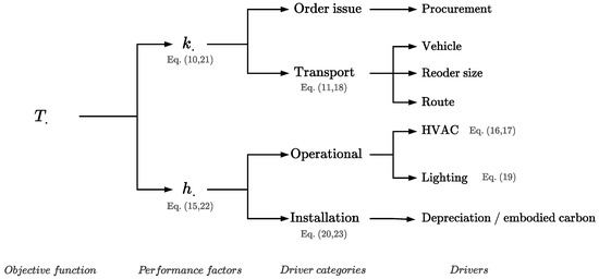
Figure 1.
Representation of the driver and driver categories for each performance factor of cost or carbon emissions.
4.2. Factor Modeling
Based on the above discussion of inventory factors for economic and environmental performance, this section presents the proposed modeling approach for the related drivers. The aim in this portion of the formulation is to consider all the determinants for costs and emissions that are relevant for inventory decisions, with a focus on different driver components and how to estimate them.
Regarding the economic perspective, the cost factor for resupply is modeled following the previously presented identification as a function of the reorder quantity Q. This factor measures the cost related to each reorder, which encompasses both order issue, with a fixed contribution , and transport. The latter () depends on the reorder quantity. The resulting formulation for cost per reorder , incurred at each inventory cycle, is
The contribution of the decision variable of reorder quantity relates to the transport driver category and it is twofold. Firstly, larger order sizes might need multiple shipments depending on vehicle capacity. Secondly, transport efficiency is affected by the weight cost factor per unit distance. More specifically, the transport component is affected directly by freight characteristics as follows:
where D is the travel distance for a single shipment, the cost weight factor, and the capacity of items per shipment. Additionally, the freight route has an additional impact other than distance: the travel speed. This affects the baseline cost per unit distance parameter .
In particular, the parameter can be estimated as being proportional to the fuel consumption via the cost per fuel volume. Following the formulation of [34], the fuel consumption per unit distance is estimated as follows:
where is the power required depending on vehicle speed, estimated as in Equation (13), assuming a constant travel speed and null road angle. The other parameters are reported in Table 2.
Table 2.
Notation for freight fuel consumption estimation.
Moreover, the coefficients related to the transported weight for each shipment are estimated as proportional to the contribution to fuel consumption per unit distance of every product of mass , given by
Regarding the cost performance factor for storage , the cost per unit time for each product stored is modeled taking into consideration the various drivers that allow for maintaining an inventory in a warehouse. These drivers make cost factors dependent on problem characteristics such as warehouse location, building characterization, and warehouse system requirements. Firstly, a warehouse needs to maintain a working environment in terms of temperature. Another operational driver considered in the storage performance factors is lighting, needed for keeping a warehouse operational. While these drivers are linked to operational aspects of the warehouse, installation costs also need to be considered through depreciation of the building and its material handling systems. The resulting cost for storage is modeled as
where , , and are the overall energy requirements per unit of time for heating, air conditioning, and lighting, respectively. These contributions, linked to costs with the factors of cost per electricity and gas , together with installation and management costs per unit of time , are repartitioned for a product with unit volume v per unit over the available storage space usable for that product V.
Regarding the first drivers for the operational category, the technique of degree days is used to estimate the energy requirements for heating a building and for air conditioning for temperature control. Degree days are defined as the sum of temperature differences between a set-point and reference temperatures [35], and are dependent on building location due to temperature variations. CIBSE [36] underline how the heat loss of a building, and thus, the required energy for the considered period, is directly proportional to this difference. Regarding heating, they link energy requirements via the heating degree days (HDDs) with the building heat loss coefficient as follows:
On the other hand, for air conditioning they formulate energy requirements as proportional to the air flow rate and air specific heat via the cooling degree days (CDDs):
Specifically, and are the efficiency coefficients for the heating system and the air conditioning, respectively, and t the total operative hours per unit time.
Moreover, according to [36], the overall heat loss coefficient is the result of the thermal characterization of the building elements (i.e., floor, roof, walls), and the air infiltration rate N:
In particular, each building element’s thermal conductance is given by its surface A and its thermal transmittance U.
Additionally, as different warehouses and inventory systems may require different lighting conditions [37], it is important to consider this driver for the performance of the inventory in terms of both costs and emissions. In particular, the resulting energy required for a lighting system is modeled as
which links the lighting requirements of the warehousing system via required illuminance L to the related estimated energy needs, considering a floor area A and a luminous efficacy for the lighting system F.
Paired with the operating cost components, the installation costs and additional management costs are another driver category. The drivers related to installation costs are related to construction, land purchasing, permission fees, and forklift flee purchasing [38], and are related to facility lifetime p. Additionally, management costs can be incurred in the considered time horizon, thus contributing to total cost per unit time:
Emission factors share similar drivers as the cost components. In particular, emissions for each resupply cycle are again influenced by a fixed () and a transport component ():
Specifically, is the emission per unit distance, which is a function of average travel speed, and , the weight factor that influences transport emissions. In particular, as mentioned previously, the variable of reorder quantity affects the transport emissions because of the number of required shipments, but also due to the degradation in performance related to increasing transported weight. These emission parameters for transport are estimated as proportional to the fuel consumption estimations of Equation (12) and Equation (14), respectively, via the carbon emissions incurred per fuel volume.
From the operating phase perspective, a warehouse contributes to the emissions of storage via the required energy for keeping it operational (i.e., for heating, air conditioning, and lighting) as follows:
where facility embodied carbon defines the emissions per unit time related to construction and installation, and the operational drivers are related to the previously defined energy consumption of heating and air conditioning, lighting, and cold rooms via the emission factors for electricity and gas .
More specifically, total embodied carbon refers to the contribution of each warehouse building element i to embodied carbon , since each building element is constituted of different materials and quantities. The resulting contribution of this driver to the storage emissions is
where the embodied carbon of each building element depends on the related material characterization. Through the identification of the constitutuent materials of each building element, both thermal and embodied carbon characterization can be performed for the warehouse building.
5. Results
The presented model and bi-objective resolution methodology aim to enhance sustainability in the reordering process, considering a comprehensive estimation of the environmental and cost inventory factors. The application of this approach is illustrated through representative scenarios for an industrial case study. This section is dedicated to demonstrating the model’s outcomes. Subsequently, through the comparison of other realistic scenarios, additional findings and insights are derived for further analysis.
5.1. Case Study
The examined case study relates to a distribution company operating regionally in Europe from one distribution center. The considered products are suitable for regular storage conditions. The warehouse, utilizing wide aisle storage with 4000 pallet places, plays a crucial role in receiving, storing, and distributing products, mainly to retailers. To sustain the operations of the distribution center, annual costs for storage are incurred due to energy consumption and depreciation of both the warehouse building and material handling equipment. Additionally, the company sustains costs for procurement, covering personnel and overhead costs.
The comprehensive consideration of overall storage and procurement costs serves as the foundation for deriving cost performance factors. Specifically, focusing on one of the company’s most representative products, the aim is to showcase the results of the bi-objective inventory-constrained optimization. In particular, historical demand data are used to estimate expected demand and the distribution . Additionally, the parameters for the estimation of environmental performance factors are approximated with the assistance of pertinent contributions from the literature that offer insights into analogous warehouse scenarios.
5.2. Estimation of Performance Factors
The determination of the cost and emission performance factors related to the inventory of the case study is performed following the identification of the drivers modeled in Section 4.2. The aim is to identify the parameters related to the cost and emission drivers in order to have all the necessary inputs for the inventory optimization problem. Table 3 summarizes all the computed input parameters, presented in detail in the remainder of this section.
Table 3.
Resulting inventory parameters used for the multi-objective inventory optimization.
Regarding the reordering portion of the model, goods are transported by road with a regional tautliner, characterized by the parameters reported in Table 4. The related estimation of the transport factors for both costs and emissions is the result of the product of fuel consumption and the cost or carbon emissions per fuel volume. In particular, it is assumed that each liter of diesel fuel is related to the emission of 2.32 kgCO2 [34] and its cost is EUR 1.5. The other component of reordering costs, given by the order issue factor , is computed for the case study company as the total procurement office costs per year, including personnel and other fixed costs, divided by the average resupply orders per year estimated from historical data. The dual factor for emissions is similarly estimated considering the emissions per office worker per year of Wilkinson and Reed [39], resulting in a fixed contribution of EUR 3.32 and 0.17 kgCO2 per replenishment. These computations allow for the estimation of the overall inventory performance factors related to reordering for both objectives, which are estimated using Equations (11) and (21), with supply route distance and speed estimated from the case study supplier location for the analyzed product.
Table 4.
Vehicle and transport data.
Concerning the storage aspect of the inventory, warehouse location plays a relevant role in operational energy requirements. For the analyzed case study, the operational energy required for space heating and cooling degree days is estimated for 80 h of operations per week [41] by using the global dataset for degree days provided by Mistry [42]. Baseline temperatures of 17 °C and 22 °C for heating and cooling are assumed, resulting in the degree day values reported in Table 5, computed as the average values over the last five years of the dataset. Regarding building characterization, the materials and thermal characteristics for each building element follow the base case of Cook and Sproul [43]. The resulting values of each storage driver, paired with the warehouse dimensions of the presented case study and embodied carbon values per major building material, allow for the estimation of storage costs and emissions. Assuming a cost of energy of EUR 28.9 for electricity and 11.9 for gas per 100 kWh [44], the resulting cost performance factor is EUR 2.28 per year for each item. Similarly, the emissions of each unit of product stored for the planning horizon of one year is 13.1 kgCO2, assuming 0.793 and 0.605 kgCO2 of emissions per kWh for electricity and gas, respectively [37].
Table 5.
Storage data.
5.3. Solution Approach
In order to tackle the multi-objective problem, the objective functions, each detailed with the respective performance factors estimated previously, are implemented within a non-dominated sorting algorithm. The goal is to identify all the feasible non-dominated solutions, which are the possible candidates for the decision variables of inventory management depending on the decision maker. This kind of transparent approach allows for taking into account all performance measures as equally important. While a single-objective policy can be optimally solved analytically for exponentially distributed lead time demand [47], more general distributions and service level constraints require numerical methods. Moreover, a multi-objective problem is considered. For these reasons, the non-dominated sorting genetic algorithm II (NSGA-II) [48] was employed for the problem resolution with the use of the Pymoo framework [49]. This evolutionary multi-objective algorithm, that has been proved to be good for two or three objectives, is based on ranking of the solutions through Pareto-dominance relations while considering the crowding distance measure to ensure solution diversity [50].
Since stockouts are modeled via service level constraints, the decision space that defines feasible solutions is restricted. With respect to this, two different service level functions are implemented and compared, namely, ready rate and fill rate. The constrained minimization problem of Equations (1) and (2) takes into account the ready rate and fill rate functions of Equations (8) and (9), respectively, as service level perspectives.
5.4. Multi-Objective Results
The constrained optimization problem for the policy, paired with the estimated parameters of Section 5.2, is tackled with the goal of identifying the Pareto frontier for the presented case study through the approach to multi-objective optimization in Section 5.3.
More specifically, the goal is to optimize the inventory of a product over a yearly horizon given the target values for the ready rate and fill rate for the service level. The parameters of the product analyzed are reported in Table 6, where and refer to the shape and scale parameters of the distribution of demand during the lead time, estimated from historical sales data.
Table 6.
Product data.
5.4.1. Service Level Constraints
When dealing with stockout behavior, it is important to examine inventory shortages from multiple service level perspectives. A service level constrained approach requires inputs for the desired service level to be maintained by the inventory, which restricts the decision space for the inventory variables. Figure 2 illustrates how different values of ready rate and fill rate influence the decision space for reorder quantity Q and level r. Notably, the figure underscores the significant influence of potentially arbitrary choices in input service level values () on the decision space, showcasing distinct effects. Namely, for the considered case study, lower values of ready rate constrain the choice of reorder quantity and level more than ready rate (Figure 2a). Moreover, Figure 2b,c highlight how high fill rates affect the choices of both inventory variables depending on the desired service level values, unlike with ready rate that sets a lower bound for reorder level. Furthermore, even when both measures can share a similar percentage input service level, considerable differences in the available decision space may arise, potentially leading to divergent inventory behavior.
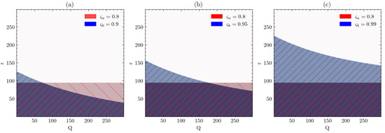
Figure 2.
Decision space for varying values of input fill rate (blue), with ready rate (red) : (a) , (b) , and (c) .
The resulting efficient solutions for the tackled multi-objective problem may be constrained by either or both service level measures depending on the related input values. Moreover, the efficient pairs and the related inventory performance may change depending on the stockout assumption; namely, if shortages can lead to backlogging of customer orders or if they lead to lost sales. As depicted in Figure 3c, the resulting Pareto frontier for the two assumptions differs. This may be due to the fact that stockouts are contrasted solely via service level constraints with the same target values; therefore, the impact on costs of stockouts is not considered and it would be different in the two scenarios. Moreover, it appears that the efficient frontiers in the objective space when considering only one service level perspective differ significantly. This may be the result of the different way that each measure constrains the decision space. Namely, the ready rate introduces a lower bound for r, while the fill rate constrains both r and Q.
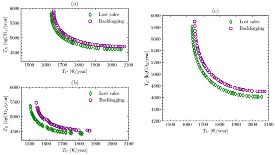
Figure 3.
Pareto frontiers for lost sales and backlogging assumptions for (a) , (b) , and (c) .
5.4.2. Warehouse Location
Another analyzed aspect is the location of the warehouse, since this affects different performance factor drivers. Specifically, while keeping the supplier location constant, this affects the transport components due to changes in transport distance and travel speed. From the storage perspective, operational emissions are impacted due to the variation in degree days, assuming constant baseline temperatures. The resulting parameters are reported in Table 7, where only the affected factors are reported.
Table 7.
Resulting inventory parameters for the different warehouse location scenario.
Notably, the change in building location results in a significant increase in transport cost and emissions, mainly due to the increase in transport distance. This causes the efficient solutions to shift to higher reorder quantity values. Other minor changes affect the storage cost and emission performance factors due to the changes in both heating and cooling energy requirements.
In order to highlight the importance of the transport component on inventory choices and performance, two scenarios are compared. Namely, the baseline vehicle capacity is compared with a reduction in of 50%. This is performed for both the studied warehouse locations. Figure 4 shows the resulting efficient solution in the objective space, where is the reduced shipment capacity. The difference in warehouse location plays a big role in the optimal choice of the reorder quantity for the economic anchor point, restricting the efficient solutions if transport capacity results are reduced. In particular, it can be observed how efficient solutions for a different warehouse location are determined by a different value of the reorder quantity. This aspect is shown from the anchor points of Figure 4b. Moreover, the objective space highlights the effect of this system characteristic on total costs and emissions. Similarly to Figure 3c, it can be observed that for the case study parameters the ready rate restricts the decision space by directly constraining the reorder level. These results confirm the need to consider sustainability perspectives as separate in order to address the issue of trade-offs between them. Additionally, considering the customer service level as another perspective via constraints allows for more comprehensive inventory decisions.
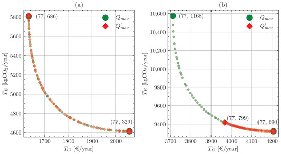
Figure 4.
Efficient solutions for (a) the original warehouse location and (b) the modified one. Pairs of optimal values for both objective functions are shown for the anchor points.
6. Conclusions
This study has focused on the modeling and optimization of a sustainable reorder-level lot-sizing policy, contributing to the literature on green supply chain optimization. The primary objective of integrating a detailed estimation of environmental factors as a baseline for comprehensive green performance assessment has been showcased within the multi-objective-constrained problem for green inventory optimization. These aspects allow for achieving efficiency of inventory management both in terms of economic and environmental performance. Moreover, the explicit multi-objective resolution approach for the constrained problem improves decision-making transparency by highlighting the trade-offs between the considered objectives. Beyond operational considerations such as energy consumption for lighting and thermal control within the warehouse, the characterization of the building and its associated embodied carbon constitute sources of carbon emissions.
The results show how some warehousing system characteristics can have an effect on multiple performance factors, and thus, affect the efficient solutions. Other primary factors affecting inventory decision are transport characteristics such as capacity, and warehouse aspects, influenced mainly by warehouse location and building characterization. Depending on the warehousing and trans-shipment context in real scenarios, different drivers may contribute to a different degree to the sustainability perspectives. The identification of major contributors to economic and environmental sustainability of an inventory system allows for the selection of efficient variables, but also highlights possible future areas of focus for more strategic decisions for companies. Additionally, the proposed approach for more comprehensive consideration of customer service metrics allows for capturing factors that may indirectly hinder company performance.
The considerations enabled by the proposed approach contribute to informed decision making in inventory control, taking into account a holistic inclusion of environmental and cost-related elements. Even though the proposed framework of sustainability drivers is general, one limitation of the study is that the estimations of cost and emission drivers may be adapted to specific real scenarios if needed, as other drivers might be present for some businesses. To further improve the decisions and insights obtainable from a model such as the one presented, a detailed analysis of the interplay between various environmental factors could be explored. This may provide valuable managerial insights for green inventory control. For example, the effect of electric vehicles on the set of efficient solutions could be analyzed. Moreover, further research could focus on widening the service level perspectives via the inclusion of other functions and the integration of performance factor estimation in other inventory policies. Other possible sustainability aspects may be addressed for a more general multi-objective inventory problem. For example, waste can be a major focus for some supply chains.
Author Contributions
Conceptualization, M.G., F.P., and M.B.; methodology, M.G., F.P., and M.B.; software, M.G.; formal analysis, M.G., F.P., and M.B.; investigation, M.G.; data curation, M.G.; writing—original draft preparation, M.G.; writing—review and editing, F.P. and M.B.; visualization, M.G.; supervision, F.P. and M.B.; project administration, F.P.; funding acquisition, F.P. All authors have read and agreed to the published version of the manuscript.
Funding
This research activity is co-funded by the Doctoral Programme “Dottorati su tematiche green” of the National Operative Program (NOP) on Research and Innovation 2014–2020.
Institutional Review Board Statement
Not applicable.
Informed Consent Statement
Not applicable.
Data Availability Statement
Data is contained within the article.
Conflicts of Interest
The authors declare no conflicts of interest. The funders had no role in the design of the study; in the collection, analyses, or interpretation of data; in the writing of the manuscript; or in the decision to publish the results.
References
- Nielsen, C. ESG Reporting and Metrics: From Double Materiality to Key Performance Indicators. Sustainability 2023, 15, 16844. [Google Scholar] [CrossRef]
- Demir, E.; Bektaş, T.; Laporte, G. A review of recent research on green road freight transportation. Eur. J. Oper. Res. 2014, 237, 775–793. [Google Scholar] [CrossRef]
- Utama, D.M.; Widodo, D.S.; Ibrahim, M.F.; Hidayat, K.; Dewi, S.K. The Sustainable Economic Order Quantity Model: A Model Consider Transportation, Warehouse, Emission Carbon Costs, and Capacity Limits; IOP Publishing Ltd.: Bristol, UK, 2020; Volume 1569. [Google Scholar] [CrossRef]
- Bonney, M.; Jaber, M.Y. Environmentally responsible inventory models: Non-classical models for a non-classical era. Int. J. Prod. Econ. 2011, 133, 43–53. [Google Scholar] [CrossRef]
- Buffa, F.P.; Reynolds, J.I. The inventory-transport model with sensitivity analysis by indifference curves. Transp. J. 1977, 17, 83–90. [Google Scholar]
- Chen, F.Y.; Krass, D. Inventory models with minimal service level constraints. Eur. J. Oper. Res. 2001, 134, 120–140. [Google Scholar] [CrossRef]
- Walton, S.V.; Handfield, R.B.; Melnyk, S.A. The green supply chain: Integrating suppliers into environmental management processes. Int. J. Purch. Mater. Manag. 1998, 34, 2–11. [Google Scholar] [CrossRef]
- Salas-Navarro, K.; Serrano-Pájaro, P.; Ospina-Mateus, H.; Zamora-Musa, R. Inventory Models in a Sustainable Supply Chain: A Bibliometric Analysis. Sustainability 2022, 14, 6003. [Google Scholar] [CrossRef]
- Becerra, P.; Mula, J.; Sanchis, R. Green supply chain quantitative models for sustainable inventory management: A review. J. Clean. Prod. 2021, 328, 129544. [Google Scholar] [CrossRef]
- Kwak, J.K. An Order-Up-to Inventory Model with Sustainability Consideration. Sustainability 2021, 13, 13305. [Google Scholar] [CrossRef]
- Žic, J.; Žic, S.; Đukić, G.; Dabić-Miletić, S. Exploring Green Inventory Management through Periodic Review Inventory Systems—A Comprehensive Literature Review and Directions for Future Research. Sustainability 2024, 16, 5544. [Google Scholar] [CrossRef]
- Escalona, P.; Araya, D.; Simpson, E.; Ramirez, M.; Stegmaier, R. On the shortage control in a continuous review (Q, r) inventory policy using αl service-level. RAIRO-Oper. Res. 2021, 55, 2785–2806. [Google Scholar] [CrossRef]
- Gonçalves, J.N.; Carvalho, M.S.; Cortez, P. Operations research models and methods for safety stock determination: A review. Oper. Res. Perspect. 2020, 7, 100164. [Google Scholar] [CrossRef]
- Daryanto, Y.; Wee, H.M.; Wu, K.H. Revisiting sustainable EOQ model considering carbon emission. Int. J. Manuf. Technol. Manag. 2021, 35, 1–11. [Google Scholar] [CrossRef]
- Fleischmann, M.; Bloemhof-Ruwaard, J.M.; Dekker, R.; Van der Laan, E.; Van Nunen, J.A.; Van Wassenhove, L.N. Quantitative models for reverse logistics: A review. Eur. J. Oper. Res. 1997, 103, 1–17. [Google Scholar] [CrossRef]
- Cárdenas-Barrón, L.E. The economic production quantity (EPQ) with shortage derived algebraically. Int. J. Prod. Econ. 2001, 70, 289–292. [Google Scholar] [CrossRef]
- Grubbström, R.W.; Erdem, A. The EOQ with backlogging derived without derivatives. Int. J. Prod. Econ. 1999, 59, 529–530. [Google Scholar] [CrossRef]
- Tao, S.; Liu, S.; Zhou, H.; Mao, X. Research on Inventory Sustainable Development Strategy for Maximizing Cost-Effectiveness in Supply Chain. Sustainability 2024, 16, 4442. [Google Scholar] [CrossRef]
- Bijvank, M.; Vis, I.F. Lost-sales inventory systems with a service level criterion. Eur. J. Oper. Res. 2012, 220, 610–618. [Google Scholar] [CrossRef]
- Digiesi, S.; Mossa, G.; Mummolo, G. A sustainable order quantity model under uncertain product demand. Ifac Proc. Vol. (IFAC-PapersOnline) 2013, 46, 664–669. [Google Scholar] [CrossRef]
- Kazemi, N.; Abdul-Rashid, S.H.; Ghazilla, R.A.R.; Shekarian, E.; Zanoni, S. Economic order quantity models for items with imperfect quality and emission considerations. Int. J. Syst. Sci. Oper. Logist. 2018, 5, 99–115. [Google Scholar] [CrossRef]
- Tiwari, S.; Daryanto, Y.; Wee, H.M. Sustainable inventory management with deteriorating and imperfect quality items considering carbon emission. J. Clean. Prod. 2018, 192, 281–292. [Google Scholar] [CrossRef]
- Marta, M.; Belinda, L.M. Simplified model to determine the energy demand of existing buildings. Case study of social housing in Zaragoza, Spain. Energy Build. 2017, 149, 483–493. [Google Scholar] [CrossRef]
- Qin, J.; Bai, X.; Xia, L. Sustainable Trade Credit and Replenishment Policies under the Cap-And-Trade and Carbon Tax Regulations. Sustainability 2015, 7, 16340–16361. [Google Scholar] [CrossRef]
- Ma, X.; Ji, P.; Ho, W.; Yang, C.H. Optimal procurement decision with a carbon tax for the manufacturing industry. Comput. Oper. Res. 2018, 89, 360–368. [Google Scholar] [CrossRef]
- Yang, H.; Luo, J.; Wang, H. The role of revenue sharing and first-mover advantage in emission abatement with carbon tax and consumer environmental awareness. Int. J. Prod. Econ. 2017, 193, 691–702. [Google Scholar] [CrossRef]
- Hovelaque, V.; Bironneau, L. The carbon-constrained EOQ model with carbon emission dependent demand. Int. J. Prod. Econ. 2015, 164, 285–291. [Google Scholar] [CrossRef]
- Bouchery, Y.; Ghaffari, A.; Jemai, Z.; Dallery, Y. Including sustainability criteria into inventory models. Eur. J. Oper. Res. 2012, 222, 229–240. [Google Scholar] [CrossRef]
- Bozorgi, A.; Pazour, J.; Nazzal, D. A new inventory model for cold items that considers costs and emissions. Int. J. Prod. Econ. 2014, 155, 114–125. [Google Scholar] [CrossRef]
- Žic, J.; Žic, S. Multi-criteria decision making in supply chain management based on inventory levels, environmental impact and costs. Adv. Prod. Eng. Manag. 2020, 15, 151–163. [Google Scholar] [CrossRef]
- Pilati, F.; Giacomelli, M.; Brunelli, M. Environmentally sustainable inventory control for perishable products: A bi-objective reorder-level policy. Int. J. Prod. Econ. 2024, 274, 109309. [Google Scholar] [CrossRef]
- Chiu, H.N. An approximation to the continuous review inventory model with perishable items and lead times. Eur. J. Oper. Res. 1995, 87, 93–108. [Google Scholar] [CrossRef]
- Silver, E.A.; Pyke, D.F.; Thomas, D.J. Inventory and Production Management in Supply Chains; CRC Press: Boca Raton, FL, USA, 2017; p. 261. [Google Scholar] [CrossRef]
- Bektaş, T.; Laporte, G. The Pollution-Routing Problem. Transp. Res. Part B Methodol. 2011, 45, 1232–1250. [Google Scholar] [CrossRef]
- Christenson, M.; Manz, H.; Gyalistras, D. Climate warming impact on degree-days and building energy demand in Switzerland. Energy Convers. Manag. 2006, 47, 671–686. [Google Scholar] [CrossRef]
- CIBSE. Degree-Days: Theory and Application; CIBSE: London, UK, 2006. [Google Scholar]
- Ries, J.M.; Grosse, E.H.; Fichtinger, J. Environmental impact of warehousing: A scenario analysis for the United States. Int. J. Prod. Res. 2017, 55, 6485–6499. [Google Scholar] [CrossRef]
- Accorsi, R.; Bortolini, M.; Gamberi, M.; Manzini, R.; Pilati, F. Multi-objective warehouse building design to optimize the cycle time, total cost, and carbon footprint. Int. J. Adv. Manuf. Technol. 2017, 92, 839–854. [Google Scholar] [CrossRef]
- Wilkinson, S.J.; Reed, R.G. Office building characteristics and the links with carbon emissions. Struct. Surv. 2006, 24, 240–251. [Google Scholar] [CrossRef][Green Version]
- Goeke, D.; Schneider, M. Routing a mixed fleet of electric and conventional vehicles. Eur. J. Oper. Res. 2015, 245, 81–99. [Google Scholar] [CrossRef]
- Fichtinger, J.; Ries, J.M.; Grosse, E.H.; Baker, P. Assessing the environmental impact of integrated inventory and warehouse management. Int. J. Prod. Econ. 2015, 170, 717–729. [Google Scholar] [CrossRef]
- Mistry, M.N. A high-resolution (0.25 degree) historical global gridded dataset of monthly and annual cooling and heating degree-days (1970–2018) based on GLDAS data [dataset]. PANGAEA 2019. [Google Scholar] [CrossRef]
- Cook, P.; Sproul, A. Towards low-energy retail warehouse building. Archit. Sci. Rev. 2011, 54, 206–214. [Google Scholar] [CrossRef]
- Eurostat. Electricity and Gas Prices Stabilise in 2023. 2023. Available online: https://ec.europa.eu/eurostat/en/web/products-eurostat-news/w/ddn-20231026-1 (accessed on 8 January 2024).
- Szokolay, S. Introduction to Architectural Science; Routledge: London, UK, 2012. [Google Scholar] [CrossRef]
- Hammond, G.; Jones, C. Embodied Carbon: The Inventory of Carbon and Energy (ICE); Lowrie, F., Tse, P., Eds.; BSRIA: Bracknell, UK, 2011; p. 128. [Google Scholar]
- Namit, K.; Chen, J. Solutions to the inventory model for gamma lead-time demand. Int. J. Phys. Distrib. Logist. Manag. 1999, 29, 960–995. [Google Scholar] [CrossRef]
- Deb, K.; Pratap, A.; Agarwal, S.; Meyarivan, T. A fast and elitist multiobjective genetic algorithm: NSGA-II. IEEE Trans. Evol. Comput. 2002, 6, 182–197. [Google Scholar] [CrossRef]
- Blank, J.; Deb, K. Pymoo: Multi-Objective Optimization in Python. IEEE Access 2020, 8, 89497–89509. [Google Scholar] [CrossRef]
- Pang, L.M.; Ishibuchi, H.; Shang, K. NSGA-II with simple modification works well on a wide variety of many-objective problems. IEEE Access 2020, 8, 190240–190250. [Google Scholar] [CrossRef]


Disclaimer/Publisher’s Note: The statements, opinions and data contained in all publications are solely those of the individual author(s) and contributor(s) and not of MDPI and/or the editor(s). MDPI and/or the editor(s) disclaim responsibility for any injury to people or property resulting from any ideas, methods, instructions or products referred to in the content. |
© 2024 by the authors. Licensee MDPI, Basel, Switzerland. This article is an open access article distributed under the terms and conditions of the Creative Commons Attribution (CC BY) license (https://creativecommons.org/licenses/by/4.0/).