Analysis of the Spatio-Temporal Differences and Structural Evolution of Xizang’s County Economy

Abstract

County’s level economic disparities remain as a key policy issue for sustainable and healthy regional development, particularly for their spatiotemporal dynamics. This research adopted Geographic Information Systems software and spatial econometric analysis methods to analyze the temporal and spatial disparities, spatial structures, and dynamic evolution processes of the Xizang Autonomous Region’s county-level economy. With the application of the coefficient of variation and spatial autocorrelation methods, the research identified a significant trend of narrowing economic differences among the 74 counties. The study also observes a growing spatial autocorrelation, pointing towards a more clustered economic growth pattern, particularly influenced by the Lhasa economic circle’s expanding regional radiation capacity. The findings underscore the importance of strategic development planning, including the integrated development of Lhasa and Shannan. This study contributes to the literature on regional economic development and offers insights for policy formulation aimed at sustainable and equitable growth in Xizang, which could also benefit future development of counties in developing countries with comparable economic environments.

1. Introduction

County economies are defined by administrative boundaries, forming a distinct type of regional economy that embodies both urban and rural economies [1,2]. The per capita GDP serves as a common metric for assessing a county’s economic development level. However, it’s important to consider that in less developed regions, higher convergence rates can lead to more rapid economic progress. This underscores the need to analyze regional disparities and the processes of economic convergence within the context of cross-sectional data [3]. Such analysis is essential for understanding the dynamic economic landscapes across different counties, taking into account their distinct developmental stages and the potential for growth and integration. Besides, county economic inequality has always been a policy issue for sustainable and healthy regional development, especially in a transitional country such as China [4,5]. the county economy represents a particular scale of economic organization [6]. From the perspective of location factors, it can be divided into areas with superior location and areas with inferior location. Superior location refers to counties located near transportation hubs, major cities, and ports, which can fully utilize surrounding advantageous resources. Inferior location refers to remote mountainous areas with inconvenient transportation, scarce resources, far from commercial centers, and lagging industrial development. This reflects the economic benefits of transport infrastructure investment [7]. The division of economic regions reveals the complete functions of spatial geographical location, regulatory entities, and market economy orientation in regional economy, affecting the income gap between urban and rural areas. Income inequality is a global issue that poses substantial challenges to social and economic development [8,9]. Income inequality remain as a major concern between urban and rural areas, especially in developing countries [10,11,12,13]. The most apparent manifestation of this inequality is the urban-rural income gap [14]. As for the scope of this research, the county economy in Xizang Autonomous Region plays a significant foundational role in the overall economic development of the region and is closely related to Xizang’s economic growth, social stability, and other aspects. However, due to the unique economic development environment, the county economy in Xizang has been relatively slow and lagging, adversely affecting aspects such as new urbanization in Xizang and the elimination of a dual economic structure. To meet the new trends in economic and social development during the “14th Five-Year Plan” period, it is necessary to accelerate the cultivation of growth poles and growth points based on county economies, thus constructing a new regional economic development pattern in Xizang supported by these poles and points.

In terms of research on county economy, some scholars have studied on the sustainable development of county economy [15], while others have studied regional economic resilience [16,17,18,19], especially methods for measuring regional economic resilience [20,21,22]. Scholars have also analyzed the factors that may affect the development of county economy from different perspectives [23,24,25,26]. Furthermore, regarding economic spatiotemporal evolution, some scholars have studied the spatiotemporal evolution of county economic growth [4], concluding that spatial agglomeration and institutional intervention can lead to spatial inequality [27,28], and the temporal dimension has also been considered [29]. Other scholars have used stochastic block models, entropy weight methods, TOPSIS methods, and the panel Tobit model to study the spatiotemporal differences of various economies [30,31,32]. With regard to Xizang’s economy, especially the county economy, scholars have studied the new situation of Xizang’s economic development in the new era [33] and poverty reduction [34,35,36], the importance of Xizang’s economic development [37,38,39], the dynamics of Xizang’s urbanization [40,41], and the energy problem of Xizang [42,43], coordinated development of environmental green [44,45,46,47], accessibility and economic development [48,49,50], the traffic dominance of Xizang [51,52], and the Hydropower of Xizang [53], the level of rural human settlement of Xizang [54,55], etc.

However, there is a scarcity of empirical studies that examine the spatial economy of Xizang’s counties through the lens of economic geography, particularly focusing on the temporal and spatial variations and the dynamic progression of the region’s economy. This research seeks to fill this gap by conducting an empirical analysis of the economic disparities and evolution over time and space in Xizang. In particular, The study intends to explore the intrinsic factors driving structural changes and the distinctive features of economic development across different periods and geographic locations within the counties of Xizang. The results would render valuable insights for the development of Xizang’s county spatial economy, which could be generalized for counties in developing countries with comparable economic environments. The structure of this paper is as follows: The first part introduces the basic concept of county economy and the necessity of research, the second part introduces the data and models used in this article, the third part analyzes the evolution of the spatio-temporal differences in Xizang’s county economy, and the fourth part discusses the results. Lastly, the final part draws conclusions.

2. Samples and Data Sources

To further study the historical development pattern of Xizang’s county economy, this study took a spatial-temporal perspective to reveal the characteristics of Xizang’s county economic development and analyze the temporal and spatial structural evolution of Xizang’s county economy. The basic data period was an annual basis with the sample data group for the years 2000 to 2019 prior to the COVID-19 to avoid inconsistencies of the economic data due to the effect of the pandemic. The data were collected from all counties in Xizang. The per capita GDP economic indicator was used to analyze the level of regional economic development [3].

In addition, considering the long-time span, and taking into account the document “State Council’s Approval for the Establishment of Shuanghu County in Xizang Autonomous Region”, the original Nima County’s Shuanghu Special Zone was established as Shuanghu County at the end of 2013 and came under the jurisdiction of Nagqu City, which was upgraded to a prefecture-level city in July 2017. We carried out statistical calculations of the relevant data for Shuanghu County after 2013 and obtained the per capita GDP data through the Xizang Autonomous Region Statistical Yearbook and relevant databases, using GIS software (version 10.3) for related calculations and analysis. The selected GIS software offers professional stability and a suite of spatial analysis tools, crucial for analyzing and accurately presenting the temporal and spatial dynamics of economic data across Xizang’s counties, while seamlessly integrating with our existing data processing workflow to enhance efficiency and accuracy [18].

3. Model Construction

3.1. Coefficient of Variation

The coefficient of variation is a statistical measure used to assess the degree of dispersion of observed values [56]. When multiple statistical measurement units cannot be compared with each other, the coefficient of variation (CV) must be used to calculate the data dispersion:

$$CV={\displaystyle \frac{1}{\overline{X}}}\times \sqrt{\left[{\displaystyle \frac{1}{n}}{\displaystyle \sum _{i=1}^n{(X_i-\overline{X})}^2}\right]}$$

(1)

In terms of time dimension, the coefficient of dispersion can be used to analyze the changes in economic data of the same region during different time periods. If the coefficient of dispersion is small, it indicates that the economic development is relatively stable and the fluctuation of growth rate is small; On the contrary, it indicates that there is significant uncertainty in economic development.

In the spatial dimension, the coefficient of dispersion can be used to compare the differences in economic data between different regions. Regions with high dispersion coefficients may have problems with imbalanced economic development, and further analysis of the reasons is needed to take corresponding policy measures. However, when calculating the correlation between the observed values of a spatial point and the observed values of its neighboring points, spatial autocorrelation statistics methods must be used. Spatial autocorrelation can be divided into global spatial autocorrelation and local spatial autocorrelation models. Through spatial autocorrelation statistics, we can examine the distribution of variables within the space and determine if spatial dependence and spatial heterogeneity exist in the spatial structure.

3.2. Spatial Autocorrelation Model

When we need to calculate the correlation between the observed values of a point in space and its adjacent points, we must use spatial autocorrelation statistical methods. Spatial autocorrelation can be further divided into two autocorrelation models: global spatial autocorrelation and local spatial autocorrelation. We can detect the distribution of variables within a space and examine whether there is spatial dependence and heterogeneity in the spatial structure by statistically analyzing spatial autocorrelation.

3.2.1. Global Spatial Autocorrelation Model

Global spatial autocorrelation reflects the overall spatial correlation trend of the observed data in the entire region [57]. We commonly use the Moran’s I statistic to measure it, with values ranging from −1 to 1.

$$I={\displaystyle \frac{n{\displaystyle \sum _{i=1}^n{\displaystyle \sum _{j=1}^n{W}_{ij}(X_{i,t}-\overline{X})(X_{j,t}-\overline{X})}}}{{\displaystyle {\sum }_{i=1}^n{\displaystyle {\sum }_{j=1}^n{(X_{i,t}-\overline{X})}^2}}}}$$

(2)

To determine if the results of global autocorrelation are significant, we usually conduct a hypothesis test by using the standardized Z value for Moran’s I to decide whether to reject or accept the hypothesis. If the Z value of Moran’s I is greater than or equal to 1.96 or less than or equal to 1.96, we consider the space to have spatial correlation. A Moran’s I value greater than zero indicates spatial positive correlation, with larger values implying more significant spatial correlation.

3.2.2. Local Spatial Autocorrelation Model

This model reflects the degree of clustering in local space, showing the degree of correlation between a small area and its adjacent local areas to infer the extent of clustering [58].

$$I_i={\displaystyle \frac{n(X_i-\overline{X})}{{\displaystyle {\sum }_{i=1}^n{(X_i-\overline{X})}^2}}}{\displaystyle {\sum }_{j=1}^n{W}_{ij}(X_j-\overline{X})}$$

(3)

Here, n represents the number of regions, X_(i,t) and X_(j,t) denote the per capita GDP values of regions i and j in year t. $\overline{X}$ is the mean per capita GDP of the research area in year t, and W_ij is the relational matrix of spatial adjacency within the research area, set as the weight matrix. I takes values between −1 and 1, with a larger I value indicating a greater positive spatial distribution correlation, a smaller I value suggesting a more random spatial distribution, and a negative value below 0 indicating a negative correlation.

In common analyses of local spatial autocorrelation clustering and outlier analysis, there are generally five types: (1) High-High (HH) type indicates hotspots, where the region itself and its surrounding areas have small differences and exhibit positive spatial autocorrelation; (2) High-Low (HL) type indicates prominent heterogeneity, with the region itself having a high level but its surrounding areas relatively low and significant negative spatial disparity; (3) Low-High (LH) type denotes a situation where the region itself has a low level while the surrounding areas have relatively higher levels and significant negative spatial disparity; (4) Low-Low (LL) type, known as blind spots, where the region and its surroundings are all low and have small spatial disparities with strong positive spatial autocorrelation; (5) Not significant type, indicating no correlation between the region itself and its surroundings.

4. Results

4.1. Evolution of Temporal and Spatial Disparities in Xizang’s County Economy

The coefficient of variation (CV) values for Xizang’s county economy were calculated using the Formula (1). Figure 1 illustrates the trend of CV values for the Xizang’s counties from 2000 to 2019 over a span of 20 years. The CV value is from 3.06 in 2000 to 2.30 in 2019, and the county economic difference in Xizang is generally decreasing. From 2000 to 2002, the dispersion coefficient seemed to be at a relatively high level. In 2001, the CV value suddenly increased, and the dispersion of Xizang’s county regional economic development suddenly increased. This is also inseparable from the tilt of relevant economic policies on the 50th anniversary of Xizang’s peaceful liberation. The CV value decreased from around 2003 to 2006, and the degree of dispersion relatively decreased. But after 2007, the CV value began to show a series of fluctuations, with an overall downward trend, indicating that the gap in county-level economic development was narrowing and the county-level economy was developing more evenly. This may be due to the government’s implementation of poverty alleviation policies, regional coordinated development policies, etc., which have promoted the economic development of underdeveloped areas and vulnerable groups.

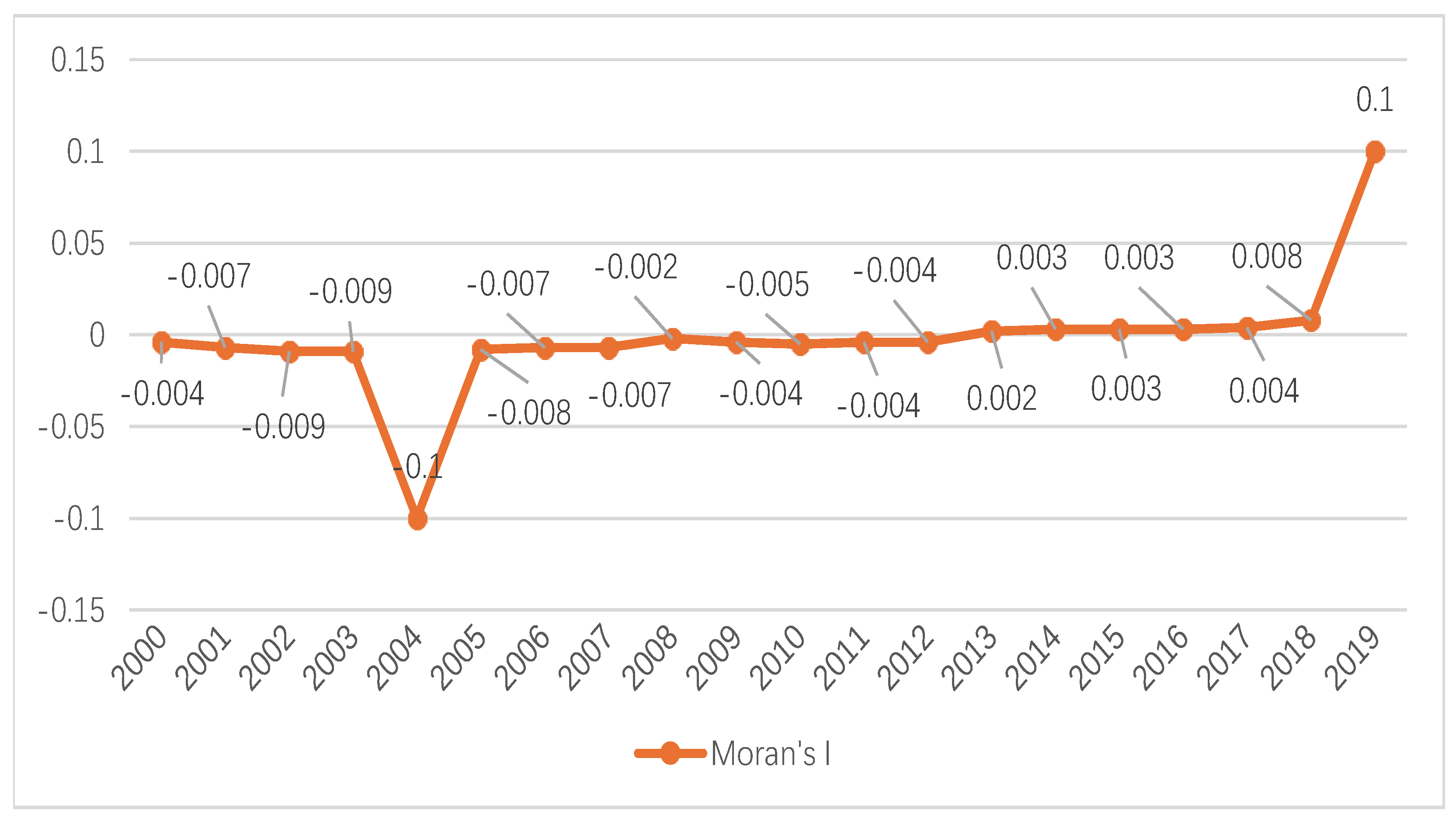
4.2. Analysis of Global Spatial Autocorrelation Differences

The ArcGIS software (version 10.3) was used to calculate the global spatial autocorrelation index of per capita GDP in Xizang’s county regions from 2000 to 2019, and the results are shown in Figure 2. The global autocorrelation index values were positive from 2000 to 2019, and the normal statistical values of Moran’s I Z-test and p-values for each year indicated significant results. This suggests that from 2000 to 2019, the per capita GDP in Xizang’s county regions exhibited a significant positive spatial autocorrelation, indicating that the county regions with higher economic development levels tended to be adjacent to each other, while the regions with lower economic levels also tended to be adjacent.

The trend in the Moran’s I curve indicates that from 2000 to 2004, the spatial agglomeration of Xizang’s county economy gradually decreased, and the neighboring effect of regional economic growth strengthened. Throughout the study period, the spatial correlation of per capita GDP exhibited small fluctuations, showing a concentrated distribution characteristic and suggesting that economic ties between counties strengthened year by year, leading to a gradual decrease in economic disparities between counties. Apart from a slight decrease in the autocorrelation value in 2007, the values gradually increased in subsequent years. However, it is important to note the year 2001 when the global autocorrelation value suddenly increased, coinciding with the 50th anniversary of the peaceful liberation of Xizang. This sudden increase could be attributed to the overall improvement in social welfare due to the 50th anniversary, leading to an increase in per capita GDP in all counties in Xizang and ultimately increasing the global autocorrelation value.

4.3. Analysis of Local Spatial Autocorrelation Differences

To further analyze the spatial development characteristics of Xizang’s county economy, this study selected five time points—2000, 2005, 2010, 2015, and 2019—as research cross-sections. The five-year plan was crucial for China’s economic strategy, and examining it over such cycles aligns research with national policies and stages. The five years like 2000, 2005, 2010, and 2015 could mark the start or end of these plans, highlighting policy shifts and economic phases. Choosing 2019 as the endpoint provided a pre-pandemic view of Xizang’s county economy, offering a clearer reflection of its development under normal conditions.

Subsequently, the Moran scatter plots of per capita GDP in Xizang’s county regions were analyzed, and the spatial pattern of Xizang’s county economy was mapped using the ArcGIS software.

According to the characteristics of local spatial autocorrelation, the economic development of Xizang’s county regions can be classified into 5 types:

(1)

High-High Type

The “High-High Type” represents a county with relatively high economic development surrounded by neighboring counties with high economic levels. Analysis of the spatial patterns from 2000 to 2010 did not exhibit the “High-High” type until 2015 when Mozhugongka County, Dazi District, and Linzhou County maintained high levels of economic development and radiation capacity, driving economic growth in neighboring areas. By 2019, only Mozhugongka County and Naidong District continued to maintain a high level of economic development.

Analysis of the spatial structure of the economy in Xizang, an counties over the past decade reveals a dynamic shift in the range of counties with high economic development levels, transitioning gradually from those belonging solely to the Lhasa region to those encompassing both Lhasa and Shannan regions. Through map analysis, it is evident that county centers exhibiting a high degree of economic development are gradually shifting from the center of the Xizangan region towards the eastern part of Xizang. Moreover, there is a gradual formation of a “high-high” correlation zone involving Lhasa and Shannan, indicating the emergence of spatially strong positive correlations, or “hotspot areas”.

This gradual formation culminates in the establishment of the “Lhasa-Shannan Economic Circle”. These developments largely align with the requirements for regional economic development outlined in the 13th Five-Year Plan for Xizang. The acceleration of infrastructure construction along the Qinghai-Xizang Railway and the “One River, Three Gorges” region has facilitated enhanced connectivity in transportation modes. Consequently, the construction of economic circles linking Lhasa to Shannan and other areas is steadily progressing. The radiating effect of the capital city on the overall development of the region continues to expand, while economic development in surrounding areas is continuously reinforced through this economic radiation.

(2)

Low-Low Type

The “low-low” type represents regions in Xizang where economic development is slow and surrounded by areas with similarly low economic development levels. From 8 counties in 2000 to 7 counties in both 2005 and 2010, and then to 11 counties in 2015 and 10 counties in 2019, we observe a trend of increasing and then gradually decreasing numbers of “low-low” type counties. This trend suggests a corresponding trend in the economic development levels of less developed regions in Xizang. Due to the influence of the radiating capacity of regions with high economic development, the number of counties categorized as “blind spots” shows a trend of initially increasing and then decreasing.

From the data, we notice a slight trend in the geographical location shifting from western and southern Xizang towards northern Xizang. Particularly, counties in the Shigatse and Ngari regions exhibit a prolonged “low-low” economic development level compared to their surrounding counties. These regions and their surrounding areas have weak economic foundations, compounded by their considerable distance from economic centers. Consequently, the radiating effects of developed regions are unable to reach these areas, and it is challenging for funds, technology, and talent to converge here. This situation leads to a widening economic gap between these areas and developed regions.

(3)

Low-High Type

The “low-high” type represents regions in which a county exhibits relatively low economic development levels while being surrounded by counties with higher economic development levels. Data indicates that the number of counties in this category increased from 14 in 2000 to 10 in both 2005 and 2010, and then further to 20 counties in 2015 and 21 counties in 2019. In terms of quantity, the number of “low-high” type counties shows a trend of initially decreasing, then increasing significantly. This trend suggests that more and more counties in Xizang are exhibiting significant spatial disparities with their surrounding counties, indicating an increasing number of counties with pronounced heterogeneity.

Analysis of the changing number and distribution of “low-high” type counties reveals that an increasing number of these counties surround parts of Lhasa, indicating that certain counties within Lhasa are experiencing much faster economic growth rates compared to their surrounding counties. This also suggests that the strong economic regions within the “high” category of the “low-high” type are driving growth in surrounding counties at a slower pace than their own growth rate. Consequently, their own economic growth capacity is expanding significantly, leading to a situation where surrounding areas become stronger while the central areas become weaker.

(4)

High-Low Type

The “high-low” type represents regions where a county exhibits relatively high economic development levels but is surrounded by counties with lower economic development levels. From 2000 to 2015, there were no counties categorized under this type, but in 2019, the Chengguan District of Lhasa was classified as such, with its economic development surpassing that of its neighboring counties. This indicates that the economic development of Chengguan District in Lhasa has grown significantly faster in recent years, and its economic growth capacity is driving the development of surrounding counties at a slower pace compared to its own development rate.

(5)

Not Significant Type

The “not significant” type refers to regions where there is no significant spatial autocorrelation among the economic development levels of various counties, and instead, the region exhibits a spatially random distribution. In the context of economic development in counties, the majority fall into this category, indicating a random distribution of county development. Based on statistical analysis of four cross-sectional data sets on economic development in counties, we can derive the local spatial autocorrelation table for counties, as shown in

Table 1. Local Spatial Autocorrelation Table for Counties in Xizang.

Year	High-High Type	High-Low Type	Low-High Type	Low-Low Type
2000	—	—	Shenzha County	Ritu County
			Bangda County	Geji County
			Nagqu County	Gajiu County
			Jiali County	Zhada County
			Gongbujiangda County	Pulan County
			Lang County	Zhongba County
			Longzi County	Jilong County
			Cuona County	Nielamu County
			Luozha County
			Cuoqin County
			Qiongjie County
			Zhanang County
			Renbu County
2005	—	—	Shenzha County	Ritu County
			Bangda County	Geji County
			Nagqu County	Gajiu County
			Jiali County	Zhada County
			Gongbujiangda County	Pulan County
			Lang County	Zhongba County
			Longzi County	Nielamu County
			Cuona County
			Sangri County
			Qusong County
2010	—	—	Shenzha County	Ritu County
			Bangda County	Geji County
			Jiali County	Gajiu County
			Gongbujiangda County	Zhada County
			Lang County	Pulan County
			Longzi County	Zhongba County
			Cuona County	Nielamu County
			Cuoqin County
			Qiongjie County
			Zhanang County
2015	Linzhou County		Bangda County	Ritu County
	Motuo County		Dangxiong County	Geji County
	Dazi County		Namling County	Gajiu County
			Nimu County	Zhada County
			Renbu County	Pulan County
			Zhanang County	Zhongba County
			Qiongjie County	Coqen County
			Qushui County	Nima County
			Gongga County	Saga County
			Langkazi County	Jilong County
			Luozha County	Nielamu County
			Cuomei County
			Qusong County
			Sangri County
			Jiacai County
			Lang County
			Longzi County
			Cuona County
			Gongbujiangda County
			Jiali County
2019	Motuo County	Chengguan District	Bangda County	Ritu County
	Naidong County		Dangxiong County	Geji County
			Namling County	Gajiu County
			Nimu County	Zhada County
			Linzhou County	Pulan County
			Motuo County	Zhongba County
			Dazi County	Coqen County
			Cuona County	Nima County
			Qiongjie County	Jilong County
			Qushui County	Nielamu County
			Gongga County
			Langkazi County
			Luozha County
			Cuomei County
			Qusong County
			Sangri County
			Jiacai County
			Lang County
			Longzi County
			Cuona County
			Gongbujiangda County
			Jiali County

.

4.4. Analysis of Dynamic Changes in Local Spatial Correlation Types

Based on the characteristics of the spatial patterns of economic development in Xizangan counties as illustrated in Figure 3, we divide them into three stages:

The Slow Growth Stage (2000–2005): During this stage, there were no changes in the “high-high” and “high-low” regions, while the number of “low-high” and “low-low” type counties slightly decreased.

The Stable Stage (2005–2010): In this period, the quantities of the four types of regions fluctuated only slightly, without significant changes.

The Leapfrog Growth Stage (2010–2019): This stage can be further divided into two sub-stages:

The First Sub-Stage: The appearance of “high-high” type counties for the first time, accompanied by relatively minor changes in the “low-high” and “low-low” types, indicating a significant improvement in the quality of development and a noticeable enhancement in economic development capabilities.

The Second Sub-Stage: The first appearance of “high-low” type counties, accompanied by a significant proportion of changes in “high-high” type counties. This suggests that while these areas are experiencing rapid economic development themselves, they are also gradually driving the development of surrounding counties, demonstrating a certain level of radiating driving force.

4.5. Analysis of the Dynamic Evolution Characteristics of Spatial Economic Structure

In our analysis of the spatial pattern of economic development in Xizangan counties over the past 20 years, we have identified the following dynamic evolution characteristics:

The “low-low” type regions are mainly concentrated in the counties of Shigatse and Ngari. Despite the gradual improvement in economic development levels in Xizangan counties over the years, the area of “low-low” type regions has shown a trend of decreasing first and then increasing. This indicates that the imbalance in economic development among Xizangan counties has become increasingly apparent in recent years.

The area of “high-high” type regions is gradually increasing, mainly concentrated around the core areas of Lhasa and Shannan. The development of these regions aligns with the objectives outlined in the national economic and social development plans during the “Twelfth Five-Year Plan” and “Thirteenth Five-Year Plan” periods for the Xizang Autonomous Region. These objectives include developing the central economic zone into a distinctive agricultural and pastoral industry belt, a characteristic boutique tourism corridor, a core area for processing industries, and a forefront for opening up to the outside world, thus forming a core economic zone. Leveraging the leading role of central and southern Xizang, efforts are made to create a 3-h economic circle radiating from Lhasa to Shigatse, Shannan, Nyingchi, and Nagqu. The radiating driving force of Lhasa as the capital city is fully utilized to establish a town network and system with Lhasa as the center, other cities as axes, and central county towns as pivots.

The “high-low” type includes Chengguan District, which exhibits strong development momentum. With the operation of airports, construction of railways, and the establishment of comprehensive transportation networks, Chengguan District is striving to achieve connectivity and industrial concentration goals. It aims to ensure its core position and radiating driving force for the development of other regions, and endeavors to construct the economic highland of central Xizang.

5. Discussions

The research has determined the spatiotemporal differences and structural evolution of economic development in 74 counties (cities) in the Xizang Autonomous Region based on endogenous effects. The coefficient of variation method and spatial autocorrelation method were adopted for the analysis between 2000 and 2019. The analysis has a couple of significant findings.

First, the economic disparities among counties in Xizang show a steady trend of narrowing. Through the calculation and analysis of the coefficient of variation, it is observed that the economic disparities among counties in Xizang have generally followed a trajectory of steady decline. Specifically, from 2000 to 2019, the coefficient of variation (CV) has consistently decreased. Although there is a slight upward trend in CV values from 2011 to 2014, overall, the trend indicates a gradual reduction in economic disparities among counties in Xizang. This finding can be supported by the economic spatial distribution in counties, which has exhibited a positive spatial autocorrelation. Over the past 20 years, counties’ economic spatial distribution has shown positive spatial autocorrelation, with the overall Moran’s I coefficient trending upwards. A comparative analysis of the trends in Moran’s I and CV values indicates that during the study period, economic development disparities among counties have decreased while spatial autocorrelation has gradually increased, with the trends of these two factors being generally opposite to each other.

Furthermore, the economic landscape of Xizang’s counties is marked by notable spatial and temporal differences, with the Lhasa economic circle exemplifying a hub of growth that radiates influence across the region. The “low-low” regions, indicating areas of persistently lower economic activity, have shown a pattern of fluctuation, while the “high-high” regions, which are economically advanced, are experiencing a modest expansion. This structural change underscores the importance of strategic planning to enhance the Lhasa economic circle’s development, integrating Lhasa and Shannan for a more cohesive economic front. By focusing on industrial clustering and leveraging Lhasa’s role as the capital city, Xizang can aspire to an economic model that is not only prosperous but also sustainable and environmentally conscious, aiming to establish a cultural and tourism epicenter in central Xizang.

Last but not least, the spatial agglomeration and dispersion of regional economies not only affect regional economic development but also alter the spatial patterns of regions. Overall, the agglomeration effect in the spatial structure of Xizang’s county-level economy is strengthening. However, at the local level, there are significant differences in the radiation capacity of economically developed counties on surrounding areas. It is necessary to strengthen the coordinated development of county-level economies. For example, enhancing the construction of key towns and county seats in Xizang could create a town system characterized by reasonable structure, strong radiation capability, and functional complementarity. This could promote equal cooperation and complementary advantages among counties. Besides, it should also focus on nurturing and developing Xizang’s transportation system to form a network of interconnected core cities with coordinated spatial layout and functional development, like upgrading of national and provincial highways in cities such as Lhasa, Shigatse, and Chamdo. This could improve the layout of transportation hubs, optimize transportation organization methods, and develop intermodal transportation services integrating roads, railways, and aviation.

6. Conclusions

The research examined of spatiotemporal disparities and structural evolution from 2000 to 2019 prior to the COVID-19 pandemic. It utilized the coefficient of variation and spatial autocorrelation methods to analyze the complex dynamics within the region’s 74 counties. The findings revealed a significant trend of reducing economic disparities among these counties, which was offset by an increasing spatial autocorrelation, suggesting a more concentrated pattern of economic development. Furthermore, the research highlighted the escalating impact of spatial spillover effects on economic growth, especially within the Lhasa economic circle. It underscored the necessity for a strategic development approach that tackles regional disparities and fosters the potential for sustainable, green economic growth.

The paper has two major theoretical contributions through regional economic development by integrating the concepts of spatiotemporal disparities and structural evolution. First, the research advances the discourse on economic geography by further clarifying how endogenous factors can influence the spatial distribution and growth patterns of regional economies [59]. The research’s use of the coefficient of variation and spatial autocorrelation methods provides a robust analytical framework that can be applied to other regions facing similar developmental challenges. Second, the study’s identification of the Lhasa economic circle’s growing influence on regional growth offers a case study in regional development dynamics, where the interplay between urban centers and their surrounding areas can be better understood and modeled. This contributes to the broader literature on economic agglomeration and the role of urbanization in economic development [60]. It has rendered a deep understanding of spatial dynamics that can lead to more equitable and sustainable economic outcomes. Practically, the paper suggests proactive planning for the development of the Lhasa economic circle, leveraging the pivotal roles of Lhasa and Shannan, and enhancing the infrastructure of key cities and counties in Xizang. This approach could establish an urban system characterized by a rational structure, robust radiating influence, and functions that complement one another. Additionally, policy makers should focus on cultivating and developing Xizang’s transportation system, forming a network of core cities, and optimizing the way of transportation organization.

Certain limitations need to be considered in this research. First, the scope of the research focused on the period before the COVID-19 pandemic, which the findings may not fully capture the most recent trends of economic disparities and spatial autocorrelation. Future studies should update the data, especially after the post COVID-19 pandemic from the year of 2023. Besides, the research does not delve deeply into the potential social and environmental impacts of such development. Future studies could explore the trade-offs between economic growth, social equity, and environmental sustainability in the context of Xizang’s unique cultural and ecological landscape. Lastly, future research should also explore the utilization of freely available applications like GeoDa or R for conducting spatial correlation analyses, assessing their efficacy as alternatives to the GIS approach.

References

1. He, S.; Liao, F.H.; Li, G. A Spatiotemporal analysis of county economy and the multi-mechanism process of regional inequality in rural, China. J. Books 2019, 111, 102073. [Google Scholar] [CrossRef]
2. Qiao, J.; Lee, Y.; Ye, X. Spatiotemporal evolution of specialized villages and rural development: A case study of Henan province. China Ann. Assoc. Am. Geogr. 2016, 106, 57–75. [Google Scholar] [CrossRef]
3. Isla-Castillo, F.; Garashchuk, A.; Podadera-Rivera, P. Cross-sectional and spatial panel data analysis of territorial economic cohesion in the European Union regions based on convergence approach: From 2 to 8 per cent? Socio-Econ. Plan. Sci. 2024, 95, 102012. [Google Scholar] [CrossRef]
4. Li, Z.; Hu, Z.; Wang, Z. The space-time evolution and driving forces of county economic growth in China from 1998 to 2015. Growth Change 2020, 51, 1203–1223. [Google Scholar] [CrossRef]
5. Wei, Y.H.D.; Ye, X.Y. Beyond convergence: Space, scale, and regional inequality in China. Tijdschr. Voor Econ. En Soc. Geogr. 2009, 100, 59–80. [Google Scholar] [CrossRef]
6. Park, J.; Feiock, R.C. Stability and change in county economic development organizations. Econ. Dev. Q. 2012, 26, 3–12. [Google Scholar] [CrossRef]
7. Rokicki, B.; Stępniak, M. Major transport infrastructure investment and regional economic development–An accessibility-based approach. J. Transp. Geogr. 2018, 72, 36–49. [Google Scholar] [CrossRef]
8. Ma, X.; Chen, D.; Lan, J.; Li, C. The mathematical treatment for effect of income and urban-rural income gap on indirect carbon emissions from household consumption. Environ. Sci. Pollut. Res. 2020, 27, 36231–36241. [Google Scholar] [CrossRef]
9. Wang, X.; Shao, S.; Li, L. Agricultural inputs, urbanization, and urban-rural income disparity: Evidence from China. China Econ. Rev. 2019, 55, 67–84. [Google Scholar] [CrossRef]
10. Gao, Y.; Zang, L.; Sun, J. Does computer penetration increase farmers’ income? An empirical study from China. Telecommun. Policy 2018, 42, 345–360. [Google Scholar] [CrossRef]
11. Xie, Y.; Zhou, X. Income inequality in today’s China. Proc. Natl. Acad. Sci. USA 2014, 111, 6928–6933. [Google Scholar] [CrossRef] [PubMed]
12. Mo, Y.; Mu, J.; Wang, H. Impact and mechanism of digital inclusive finance on the urban-rural income gap of China from a spatial econometric perspective. Sustainability 2024, 16, 2641. [Google Scholar] [CrossRef]
13. Liu, S.G.; Tang, X.W.; Zhao, Y.B. Global value chain participation, employment structure, and urban-rural income gap in the context of sustainable development. Sustainability 2024, 16, 1931. [Google Scholar] [CrossRef]
14. Lagakos, D. Urban-rural gaps in the developed world: Does internal migration offer opportunities? J. Econ. Perspect. 2020, 34, 174–192. [Google Scholar] [CrossRef]
15. Peng, Y.; Guosheng, C.; Yancai, R. The Research on the Assessment of Sustainable Development of County Economy. Energy Procedia 2011, 5, 921–925. [Google Scholar] [CrossRef]
16. Doran, J.; Fingleton, B. Employment resilience in Europe and the 2008 economic crisis: Insights from micro-level data. Reg. Stud. 2016, 50, 644–656. [Google Scholar] [CrossRef]
17. Giannakis, E.; Bruggenman, A. Economic crisis and regional resilience: Evidence from Greece. Pap. Reg. Sci. 2017, 96, 451–476. [Google Scholar] [CrossRef]
18. Song, G.; Zhong, S.; Song, L. Spatial pattern evolution characteristics and influencing factors in county economic resilience in China. Sustainability 2022, 14, 8703. [Google Scholar] [CrossRef]
19. Pendall, R.; Theodos, B.; Franks, K. Vulnerable people, precarious housing, and regional resilience: An exploratory analysis. Hous. Policy Debate 2012, 22, 271–296. [Google Scholar] [CrossRef]
20. Briguglio, L.; Cordina, G.; Farrugia, N.; Vella, S. Economic vulnerability and resilience: Concepts and measurement. Oxf. Dev. Stud. 2009, 37, 229–247. [Google Scholar] [CrossRef]
21. Martin, R.; Sunley, P.; Gardiner, B.; Tyler, P. How Regions React to Recessions: Resilience and the Role of Economic Structure. Reg. Stud. 2016, 50, 561–585. [Google Scholar] [CrossRef]
22. Wang, X.W.; Li, M.Y. Determinants of Regional Economic Resilience to Economic Crisis: Evidence from Chinese Economies. Sustainability 2022, 14, 809. [Google Scholar] [CrossRef]
23. Rupasingha, A. Religious adherence and county economic growth in the US. J. Econ. Behav. Organ. 2009, 72, 438–450. [Google Scholar] [CrossRef]
24. Davlasheridze, M.; Goetz, S.J.; Han, Y. The effect of mental health on US County economic growth. Rev. Reg. Stud. 2018, 48, 155–171. [Google Scholar] [CrossRef]
25. Xu, X.; Liu, C. Research on the impact of expressway on the county economy based on a spatial DID model: The case of three provinces of China. Math. Probl. Eng. 2021, 2021, 1–13. [Google Scholar] [CrossRef]
26. Xu, H.; Dong, R.; Cui, Y.; Zang, W. Does the Photovoltaic poverty alleviation project promote county economic development?: Evidence from 852 counties in China. Sol. Energy 2022, 248, 51–63. [Google Scholar] [CrossRef]
27. Krugman, P. The new economic geography, now middle-aged. Reg. Stud. 2011, 45, 1–7. [Google Scholar] [CrossRef]
28. Rodríguez-Pose, A. Do institutions matter for regional development? Reg. Stud. 2013, 47, 1034–1047. [Google Scholar] [CrossRef]
29. Wei, Y.D. Spatiality of regional inequality. Appl. Geogr. 2015, 61, 1–10. [Google Scholar] [CrossRef]
30. Xie, H.; Wang, W. Spatiotemporal differences and convergence of urban industrial land use efficiency for China’s major economic zones. J. Geogr. Sci. 2015, 25, 1183–1198. [Google Scholar] [CrossRef]
31. Li, B.; Shi, Z.; Tian, C. Spatio-temporal difference and influencing factors of environmental adaptability measurement of human-sea economic system in Liaoning coastal area. Chin. Geogr. Sci. 2018, 28, 313–324. [Google Scholar] [CrossRef]
32. Yu, H.; Xing, L. Analysis of the spatiotemporal differences in the quality of marine economic growth in China. J. Coast. Res. 2021, 37, 589–600. [Google Scholar] [CrossRef]
33. Dreyer, J.T. Economic Development in Tibet under the People’s Republic of China//Contemporary Tibet; Routledge: London, UK, 2017; pp. 29–151. [Google Scholar]
34. Ji, Z.; Xu, H.; Cui, Q. Tourism and poverty alleviation in Tibet, China: The role of government in enhancing local linkages. Asia Pac. J. Tour. Res. 2022, 27, 173–191. [Google Scholar] [CrossRef]
35. Pan, Y.; Zhu, J.; Zhang, Y.; Li, Z.; Wu, J. Poverty eradication and ecological resource security in development of the Tibet an Plateau. Resour. Conserv. Recycl. 2022, 186, 106552. [Google Scholar] [CrossRef]
36. Zhao, Z.; Pan, Y.; Zhang, Y.; Wu, J. The impact of poverty alleviation resettlement on the sustainable development of typical immigrated village in Tibet. J. Nat. Resour. 2022, 37, 1815–1828. [Google Scholar] [CrossRef]
37. Zhou, Z.; Gao, Y.; Dong, X.; Wang, X.; Zhang, Y.; Xiao, R.; Xiao, X.; Ye, Q. Linking Ecosystem Services and Multi-Dimensional Poverty Reduction, a Case Study in the Northwest Sichuan Plateau, Tibet, China; Elsevier BV: Amsterdam, The Netherlands, 2024. [Google Scholar] [CrossRef]
38. Wang, Y. Poverty Status and Development Dilemma in Tibet an Ethnic Areas in the Border Areas Among Gansu, Qinghai, Sichuan and Tibet//Social and Economic Stimulating Development Strategies for China’s Ethnic Minority Areas; Springer Nature Singapore: Singapore, 2023; pp. 377–391. [Google Scholar]
39. Yan, R.; Chen, R. Sustainable Development and Transformative Change of Tibe in China from 1951 to 2021. Land 2024, 13, 921. [Google Scholar] [CrossRef]
40. Fang, C. How to promote the green development of urbanization in the Tibet an Plateau? J. Geogr. Sci. 2023, 33, 639–654. [Google Scholar] [CrossRef]
41. Song, T.; Guo, Y.; Chen, W. Assembling plateau urbanism through special economic zones evidence from the an Plateau, China. Cities 2024, 149, 104982. [Google Scholar] [CrossRef]
42. Bai, C.; Zhan, J.; Wang, H.; Liu, H.; Yang, Z.; Liu, W.; Wang, C.; Chu, X.; Teng, Y. Estimation of household energy poverty and feasibility of clean energy transition: Evidence from rural areas in the Eastern Qinghai-Tibet Plateau. J. Clean. Prod. 2023, 388, 135852. [Google Scholar] [CrossRef]
43. Jiang, L.; Zhao, J.; Li, J.; Yan, M.; Meng, S.; Zhang, J.; Hu, X.; Zhong, H.; Shi, S. Household energy consumption in herders on the Qinghai–Tibet an Plateau: Profiles of natural and socio-economic factors. Energy Build. 2024, 311, 114181. [Google Scholar] [CrossRef]
44. Kan, A.; Li, G.; Yang, X.; Zeng, Y.; Tesren, L.; He, J. Ecological vulnerability analysis of Tibet an towns with tourism-based economy: A case study of the Bayi District. J. Mt. Sci. 2018, 15, 1101–1114. [Google Scholar] [CrossRef]
45. Dong, H.; Feng, Z.; Yang, Y.; Li, P.; You, Z. Dynamic assessment of ecological sustainability and the associated driving factors in Tibet and its cities. Sci. Total Environ. 2021, 759, 143552. [Google Scholar] [CrossRef]
46. Fan, W.; Meng, M.; Zhou, C. Research on the impact of economic development and environmental security on human well-being in typical cities on the Qinghai-Tibet Plateau. Environ. Dev. Sustain. 2024, 1–26. [Google Scholar] [CrossRef]
47. Hua, L.; Ran, R.; Xie, M.; Li, T. China’s poverty alleviation policy promoted ecological-economic collaborative development: Evidence from poverty-stricken counties on the Qinghai-Tibet Plateau. Int. J. Sustain. Dev. World Ecol. 2023, 30, 402–419. [Google Scholar] [CrossRef]
48. Gao, X.; Sun, D. Transport accessibility and social demand: A case study of the Tibet an Plateau. PLoS ONE 2021, 16, e0257028. [Google Scholar] [CrossRef] [PubMed]
49. Luo, M.; Li, J.; Wu, L.; Wang, W.; Danzeng, Z.; Mima, L.; Ma, R. The Spatial Mismatch between Tourism Resources and Economic Development in Mountainous Cities Impacted by Limited Highway Accessibility: A Typical Case Study of Lhasa City, Tibet Autonomous Region, China. Land 2023, 12, 1015. [Google Scholar] [CrossRef]
50. Miao, Y.; Dai, T.; Song, J. Assessing the effects of the large-scale road construction on the ethnic disparities of accessibility in Tibet from 2010 to 2020. Growth Change 2023, 54, 754–770. [Google Scholar] [CrossRef]
51. Wang, D.; Wang, K.; Wang, Z.; Fan, H.; Chai, H.; Wang, H.; Long, H.; Gao, J.; Xu, J. Spatial-temporal evolution and influencing mechanism of traffic dominance in Qinghai-Tibet plateau. Sustainability 2022, 14, 11031. [Google Scholar] [CrossRef]
52. Bedeian, A.G.; Mossholder, K.W. On the use of the coefficient of variation as a measure of diversity. Organ. Res. Methods 2000, 3, 285–297. [Google Scholar] [CrossRef]
53. Luo, W.Q.; Wang, J.B.; Yan, X.W.; Jiang, G. Unbeiling the railway traffic knowledge in Tibet: An advanced model for relational Triple extraction. Sustainability 2023, 15, 14942. [Google Scholar] [CrossRef]
54. Qin, C.; Fu, B.; Zhu, X.; Dunyu, D.; Bianba, C.; Baima, R. Spatial and temporal patterns of Hydropower development on the Qinghai-Tibet Plateau. Sustainability 2023, 15, 6688. [Google Scholar] [CrossRef]
55. Gao, B.; Hu, Z. What affects the level of rural human settlement? A Case Study of Tibet, China. Sustainability 2022, 14, 10445. [Google Scholar] [CrossRef]
56. Zhang, Y.; Niu, B.; Zhang, X. Subsidy-dominated Non-farm income improves herder household livelihoods and promotes income equality in north Tibet, China. Sustainability 2024, 16, 3681. [Google Scholar] [CrossRef]
57. Boots, B.; Tiefelsdorf, M. Global and local spatial autocorrelation in bounded regular tessellations. J. Geogr. Syst. 2000, 2, 319–348. [Google Scholar] [CrossRef]
58. Ord, J.K.; Getis, A. Local spatial autocorrelation statistics: Distributional issues and an application. Geogr. Anal. 1995, 27, 286–306. [Google Scholar] [CrossRef]
59. Stimson, R.; Stough, R.; Nijkamp, P. Endogenous regional development. In Endogenous Regional Development; Edward Elgar Publishing: Cheltenham, UK, 2011. [Google Scholar]
60. Parr, J.B. The regional economy, spatial structure and regional urban systems. Reg. Stud. 2014, 48, 1926–1938. [Google Scholar] [CrossRef]
Figure 1. Changes in CV values from 2000 to 2019.
Sustainability 16 07937 g001
Figure 2. Changes in global autocorrelation coefficient from 2000 to 2019.
Sustainability 16 07937 g002
Figure 3. Spatial pattern of county economy in Xizang.
Sustainability 16 07937 g003aSustainability 16 07937 g003b