Abstract
Accurate water quality prediction is the basis for good water environment management and sustainable use of water resources. As an important time series forecasting model, the Autoregressive Moving Average Model (ARMA) plays a crucial role in environmental management and sustainability research. This study addresses the factors that affect the ARMA model’s forecast accuracy and goodness of fit. The research results show that the sample size used for model parameters estimation is the main influencing factor for the goodness of fit of an ARMA model, and the prediction time is the main factor affecting the prediction error of the model. Constructing a stable and reliable ARMA model requires a certain number of samples for the estimation of model parameters. However, using an excessive number of samples will not further improve the ARMA model’s goodness of fit but rather increase the workload and difficulty of data collection. The ARMA model is not suitable for long-term forecasting because the prediction error of ARMA models increases with the increase of prediction time, and when the prediction time exceeds a certain limit, the fitted values of an ARMA model will almost no longer change with the time, which means the model has lost its significance of prediction. For time series with periodic components, introducing periodic adjustment factors into the ARMA model can reduce the prediction error. These findings enable environmental managers and researchers to apply the ARMA model more rationally, hence developing more precise pollution control and sustainable development plans.
1. Introduction
The sustainability of water systems is critically dependent on high-level environmental management [1], and the sustainable management of the water environment is a significant challenge faced by societies and governments [2]. Good environmental management enhances the ecosystem and helps maintain sustainable water resource supplies [3]. The basis for effective water environment management is to grasp the changing trends of water pollutants [4]; hence, water quality prediction technology, particularly water quality prediction models, is crucial for maintaining the sustainability of water systems [5]. The predictions for future water quality changes can provide technical support in many aspects of water environment sustainability, including potable water supply, aquaculture, tourism, ecosystem regulation, and so on [6]. Reliable water quality forecasting can not only help water pollution control [7,8] but also provide important guidance for water environment management and decision-making [9,10]. In order to explore the changing laws of the water environment and make accurate predictions on water quality changes, there has been significant effort from scientists and water managers towards researching water quality prediction models [11].
In general, water quality prediction models can be classified into two categories: physical models and data-driven models [12]. Physical models take into account various factors of the water systems, such as the life activities of aquatic organisms, solar radiation, rainfall, runoff, wind speed and direction, nutrients, and more. It makes the physical models able to fully simulate the water quality change process [13]; at the same time, high requirements for data consistency and data computing costs also limit the utilization of physical models [14]. For the data-driven models, the object’s change process can be simulated without knowing the detailed information of all relevant factors [15]. Within data-driven models, there are statistics-based models and Artificial Intelligence (AI)-based models [16]. Statistics-based models have the advantages of simple structure and convenient calculation. They ignore the complexity of raw data and focus on the statistical patterns of data [17]. Any model has its scope of application, and no model is omnipotent. It is essential to choose the right model for the right situation.
The Autoregressive Moving Average model (ARMA) is a representative statistics-based model. It has been among the most popular mathematical models for time series prediction in the past two decades [18]. ARMA model is widely used due to some significant advantages, including faster speed of model construction and lower data requirement [19]. Although the ARMA model was first utilized in economics [20], it has now been adopted in a much broader range of research fields. In the research field of sustainability, a great portion of the data are time series, including the power load, resource consumption, water quality change process, and so on. The unique advantages of the ARMA model have led to its widespread application in various fields related to sustainability, such as hydrology [21,22,23], meteorology [24,25,26], and environmental science [27,28,29]. The traditional ARMA model requires that the time series to be fitted must be stationary, which, to some extent, limits its scope of use. To extend the ARMA model to a non-stationary time series, the integrated process is added to the ARMA model, making it an Autoregressive Integrated Moving Average Model (ARIMA). However, the core of the ARIMA model is still the ARMA model; therefore, the study of the features of the ARMA model, specifically the elements that affect its goodness of fit and prediction error, is crucial for the appropriate use of the ARMA and ARIMA models.
After years of development, relatively standardized methods and processes such as parameter selection and optimization have been formed for the construction of the ARMA model. However, there is still a lack of in-depth research on some key issues of the ARMA model, including the influencing factors of prediction error and the relationship between the sample size required for model parameter estimation and the goodness of model fitting. Many researchers determine the sample size and prediction time based on experience, intuition, and the difficulty of data collection. The sample size or prediction time of different research cases varies greatly. The analysis of some documents shows that for monthly ARMA models (models built on the monthly dataset), the length of the sample time series used for estimating model parameters can range from 10 years [19,30,31], 20 years [32,33] to more than 40 years [23], or with the option of 5 years [34] or even short as 2 years [35]. The prediction time may span over a period of 5 years [23,34] to 7 years [19] or as short as 1 year [31,32,35] to 2 years [36]. In terms of daily models (models built on the daily dataset), the time series samples used to estimate model parameters can range from 1 year [37] to 4 years [30], while the prediction time may be as long as 7 months [38], or as short as several to 10 days [30]. According to the frequency of time series data, the ARMA or ARIMA model not only includes common monthly and daily data models but also includes annual data models [29,39], weekly data models [27], and hourly data models [40,41,42]. Within the same time period, the sample size of the time series varies with the data frequencies. If the sample size is used for comparison, in certain studies, the sample size reaches over 20,000 [41], whereas in others, it is limited to just a dozen [29], and the prediction steps range from a few steps [29] to several hundred steps [38], all with significant differences.
The emergence of the above issues involves the following key questions. It is crucial to ponder these questions for the rational application of the ARMA model.
Q.1. Relationship between the sample size and the ARMA model’s goodness of fit. Is it more advantageous to utilize a larger sample size when estimating model parameters?
Q.2. Relationship between the prediction steps and the forecast accuracy of the ARMA model. What principles should be followed in determining the number of prediction steps or prediction time?
Q.3. The unique characteristics of the ARMA model. What are the underlying mechanisms behind these characteristics?
Answering these questions holds significant value for the development of the ARMA model and its rational applications, but relatively little attention has been paid to them. In this regard, this paper aims to achieve the following research objectives:
- 1)
- Analyze how the ARMA model’s goodness of fit changes with the changes in the sample size.
- 2)
- Analyze the impact of the number of prediction steps or the prediction time on the forecast error of the ARMA model.
- 3)
- Investigate the primary elements influencing the prediction accuracy of the ARMA model and explore the internal mechanism behind them.
- 4)
- Summarize the issues that need to be paid attention to in the application of the ARMA model and provide references for the reasonable application of the ARMA model in water quality prediction, water pollution control, and sustainability.
This paper elaborates on some important features of the ARMA (ARIMA) model and their underlying mechanisms in detail. It is of great significance to guide the rational application of the ARMA (ARIMA) model. Water environment managers and sustainable policymakers can benefit from the outcomes of this study because predicting and understanding the trend of water quality changes accurately is a prerequisite for water environment management and sustainable policy making. Decision-makers and researchers may leverage the outcomes of this study for sustainable and eco-centric environmental management planning, develop strategies for enhancing water quality, and maintain the sustainability of aquatic ecosystems.
The rest of the paper is organized as follows. Section 2 briefly introduces the research methods and data sources, including the evaluation methods for the model’s goodness of fit and prediction error and the description of data sources. Section 3 provides the research results, including the structures of models used in the research and the factors affecting an ARMA model’s goodness of fit and prediction error. Section 4 discusses the characteristics and mathematical mechanisms of the ARMA model in detail and some key points to be noted in the application. Section 5 concludes the whole research work.
2. Methods and Data Sources
The main idea of this study is to combine empirical research with theoretical analysis. The construction of ARMA models involves utilizing daily and monthly mean time series data derived from the online monitoring data of the Bakou environment monitoring station of Changtan Reservoir in Zhejiang Province, China. Based on the constructed models, we analyzed how sample size and prediction time affect the goodness of fit and the forecast accuracy of the ARMA model, respectively. Then, we further explored the key features of the ARMA model and its underlying mechanism and explained some crucial points that need to be noted in the reasonable application of the ARMA model. The methods, concepts, and data sources related to the research work are elaborated in detail as follows:
2.1. Introduction to the ARMA Model
The ARMA model is a prediction model based on the dynamic dependence between the current value and the lag value of a time series. It is expressed as follows:
where yt is the current term in the time series to be fitted, c is the constant term, φ1, φ2, …, φp are the fitting parameters of the autoregressive term, θ1, θ2, …, θq are the fitting parameters of the moving average term, is the residual, L is the lag operator, and , p or q is the number of lagging operations, indicates doing p lag operations and .
The ARMA model requires that the time series to be fitted must be a stationary sequence. If we want to apply the ARMA model to a non-stationary time series, an integrated process needs to be introduced into the ARMA model, which actually uses different operations to transform the original time series into a stationary one. The ARMA model with the integrated process is the ARIMA model, and its mathematical expression is as follows.
where is the difference operator and , d is the number of differences, and .
From Equation (2), it can be seen that the core of the ARIMA model is still the ARMA process. The prediction functions of the ARIMA model are all undertaken by the ARMA process, and the integrated process is only to convert non-stationary time series into stationary series through differential operation so that ARMA can be used to predict the change of non-stationary time series. Therefore, the ARIMA model not only extends the application of the ARMA model to non-stationary time series but also has the same characteristics as the ARMA model.
ARMA model is usually recorded as ARMA (p, q), where p is the autoregressive order and q is the moving average order. In practical applications, some ARMA models may only contain the AR or MA parts. If a part is missing, it would be represented by 0. Some time series exhibit obvious periodic patterns. When predicting the change trends of such time series, a periodic adjustment factor (also known as seasonal adjustment factor) can be introduced into the ARMA model. Such ARMA models are called seasonal ARMA models or SARMA models. SARMA models are usually recorded as SARMA (p, q)(P, Q)S, where P is the seasonal autoregressive order, Q is the seasonal moving average order, and S is the length of the cycle. The SARMA model is usually used for monthly or quarterly time series, with S = 12 for monthly time series and S = 4 for quarterly time series.
The construction, prediction, and evaluation of the ARMA model mainly include four steps. (1) Stationarity test, using Augmented Dickey Fuller Test (ADF Test) to examine the stationarity of a time series. If it is not stationary, the original sequence can be transformed into a stationary sequence by introducing an integrated process. (2) Autocorrelation analysis and preliminary order determination, using autocorrelation function (ACF) and partial autocorrelation function (PACF) graphs to analyze the autocorrelation of time series, roughly determining the approximate range of p and q, and selecting several candidate models according to the tailing or truncation characteristic of ACF or PACF graphs. (3) Determining the optimal model structure and parameters, that is, finally determining the values of p and q according to the Akaike Information Criterion (AIC). (4) Model evaluation, which is evaluating the goodness of fitting and the prediction error of the model based on relevant measurement indicators. The time series analysis and model construction in this paper were completed using Eviews v10.
2.2. Akaike Information Criterion (AIC)
The Akaike Information Criterion provides a quantitative way to evaluate how well a model fits the data it was created from. AIC is used to compare different possible models and determine which one is the best fit for the data. AIC is determined by the number of independent variables employed in building the model and the maximum likelihood estimate of the model (how well the model reproduces the data). The best-fit model, as determined by AIC, is the one that explains the greatest amount of variation using the fewest possible independent variables. The formula for AIC is as follows:
where k is the number of independent variables used, and L is the log-likelihood estimate (a.k.a. the likelihood that the model could have produced the observed y-values).
AIC = 2k − 2lnL
2.3. Evaluation of Model Goodness of Fit
The goodness of fit of the model is generally evaluated by the coefficient of determination (represented by R2). However, when using multiple regression analysis, even if the goodness of fit of the model does not improve significantly, R2 may still increase with the increase of the number of explanatory variables, which results in R2 not being able to reflect the goodness of fit of the model accurately. This problem is particularly prominent in the ARMA model, as the ARMA model is essentially a multiple linear regression model with often more than one explanatory variable. To avoid this problem, the adjusted coefficient of determination (represented by ) is generally used to evaluate the goodness of fit of the ARMA model. The formula for is as follows:
where is the adjusted coefficient of determination, R2 is the coefficient of determination, T is the number of samples used for model parameter estimation, and k is the number of explanatory variables.
2.4. Evaluation of the Model Prediction Error
This study needs to compare the prediction errors of models in different situations. To avoid the impact of different units of different monitoring indicators, the mean absolute percentage error (MAPE) is used to evaluate the prediction error of the model. The formula for MAPE is as follows:
where is the measured value, is the predicted value of the model, and n is the number of predicted values of the model.
2.5. Data Sources
The research data come from the Bakou environment monitoring station of Changtan Reservoir in Taizhou, Zhejiang Province, China. Changtan Reservoir is the largest drinking water source in Taizhou City and one of the six key reservoirs in Zhejiang Province [43]. The Bakou National Environment Monitoring Station is located near the outlet of Changtan Reservoir and is the most important environment monitoring station of Changtan Reservoir. It is one of the earliest environment monitoring stations in Zhejiang Province equipped with online monitoring equipment and has relatively longer-term online monitoring data. The research data come from the online monitoring data of the station from 2012 to 2021, including six indicators: Chemical Oxygen Demand for Permanganate Method (CODMn), Dissolved Oxygen (DO), Electrical Conductivity (EC), pH, Total Nitrogen (TN) and Water Temperature (WT). DO, EC, pH, and WT were measured by an online five-parameter analyzer. TN was measured by an online automatic monitor of TN. CODMn was measured by an online automatic monitor of CODMn. The online monitoring data were sampled every 4 h. Due to instrument failure or other reasons, a small amount of data are missing or abnormal. Upon evaluation, the efficient data are not less than 96%. After pretreatment and verification, two sets of time series (time series of daily mean data and monthly mean data) are formed for the construction of the daily ARMA model and monthly ARMA model, respectively.
3. Results
3.1. The Construction of the ARMA Model
In this study, two kinds of ARMA models (daily model and monthly model) were constructed for research and analysis. Daily models were constructed based on daily average data, and monthly models were constructed based on monthly average data. The construction of the two kinds of models is described as follows.
3.1.1. The Construction of the Daily ARMA Model
The ADF test shows that the daily time series of six water quality indicators (CODMn, EC, TN, DO, pH, and WT) are all stationary. Therefore, the ARMA model can be used for modeling and prediction research. Figure 1 shows the ACF and PACF graphs of the daily time series of each indicator. From the graphs, it can be seen that the ACF of all indicators (Figure 1a–f) is tailed significantly. Most of the PACF indicators cut off after lag 3 (Figure 1g–k), while TN and WT cut off after lag 2. (Figure 1i,l). Based on the AIC criteria and the significance of each variable in the model, the optimal structures of the daily models of CODMn, EC, TN, DO, pH, and WT were determined to be ARMA (3, 0), ARMA (3, 0), ARMA (1, 0), ARMA (3, 0), ARMA (3, 0), and ARMA (2, 0) respectively.
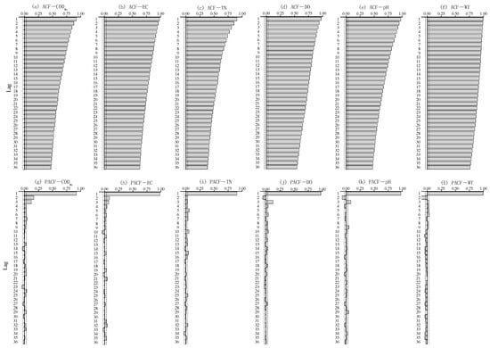
Figure 1.
ACF and PACF graphs of daily time series of water quality indicators in Changtan Reservoir.
3.1.2. The Construction of the Monthly ARMA Model
The ADF test shows that the monthly time series of six water quality indicators in Changtan Reservoir are also stationary. Figure 2 shows the ACF and PACF graph of the monthly time series of each indicator. Figure 2g–j shows that the PACF of CODMn, EC, TN, and DO cut off after lag 1, while the PACF of WT cuts off after lag 3 (Figure 2l). The PACF of pH is tailed (Figure 2k), but its ACF cuts off after lag 2 (Figure 2e). Compared to the daily time series, the autocorrelation coefficients of the monthly time series of DO, pH, and WT show significant seasonal patterns (Figure 2d–f), indicating that the seasonal adjustment factors need to be introduced into the ARMA models of the three indicators. Based on ACF and PACF graphs analysis, combined with AIC criteria, the optimal structures of monthly models of CODMn, EC, TN, DO, pH, and WT were determined to be ARMA (1, 0), ARMA (1, 0), ARMA (1, 0), SARMA (1, 0)(1, 0)12, SARMA (0, 2)(1, 0)12, SARMA (3, 0)(1, 0)12 respectively.
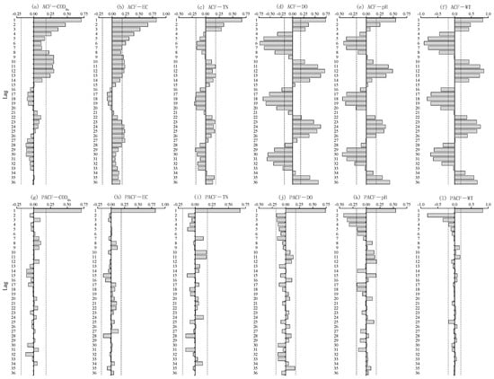
Figure 2.
ACF and PACF graphs of monthly time series of water quality indicators in Changtan Reservoir.
3.2. The Factors Affecting the ARMA Model’s Goodness of Fit and Prediction Error
3.2.1. The Impact of Past Time Series Length (Sample Size) on the ARMA Model’s Goodness of Fit
The goodness of fit reflects the degree to which the model’s fitting curve fits the variation of measured values and is an important indicator of the model’s fitting quality. Due to the fact that both the dependent and independent variables of the ARMA model come from the same time series and do not involve other exogenous variables, the number of samples used for model parameter estimation, that is, the length of the past time series is the main influencing factor affecting the model’s goodness of fit. In order to analyze the impact of sample size on the model’s goodness of fit, we calculated the of the ARMA models that were constructed based on past time series of different lengths. From Figure 3, it can be seen that whether it is the daily model or the monthly model, as the length of the past time series used for model parameter estimation increases, the overall trend of the increases. However, when the past time series reaches a certain length, the variation of tends to be relatively stable, and the generally does not continue to increase with the length of the past time series increases.
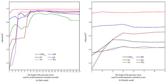
Figure 3.
Effect of the length of the past time series used for model parameter estimation on the
of ARMA models.
The length of the past time series used for model parameter estimation is a reflection of the number of samples. From Figure 3, we found that when the sample size used for model parameter estimation is small, is relatively small, indicating that the goodness of fit of the model is not ideal. Therefore, in order to build a stable and reliable ARMA model, a certain number of samples are needed to be used for model parameter estimation. However, increasing the sample size excessively cannot further improve the goodness of fit of the model. For the data in this study, when the length of the past time series of the daily model reaches about 8 months (the sample size is about 240), and the length of the past time series of the monthly model reaches about 5 years (the sample size is about 60), generally does not continue to increase with the increase in sample size. Compared to the monthly model, the parameter estimation of the daily model requires more samples in order to achieve a relatively high . This is because the data fluctuation of the daily average is greater than that of the monthly average usually. Therefore, a larger sample size is needed to reflect the daily data variation and to stabilize the model.
The sample size needed to estimate model parameters may vary for different indicators or time series, but there is still a similar pattern. Initially, as the number of samples increases, the overall goodness of fit of the model continues to improve. After exceeding a certain limit, further increasing the sample size no longer improves the goodness of fit of the model significantly.
3.2.2. The Impact of Prediction Time on the ARMA Model’s Prediction Error
Figure 4 shows the impact of prediction time on the MAPE of ARMA models. From the graphs, it can be seen that as the prediction time increases, the overall MAPE of each model shows an increasing trend. Relatively, in the initial stage of prediction, as the prediction time increases, the MAPE of the model increases rapidly. However, after the prediction time exceeds a certain limit, the variation curve of MAPE tends to flatten out and no longer increases rapidly with the increase of the prediction time.
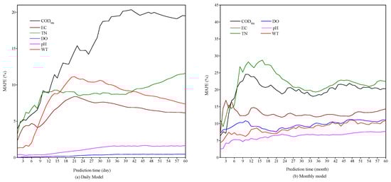
Figure 4.
The effect of prediction time on the MAPE of ARMA models.
For the data in this study, when the prediction time reaches 30 days for the daily model or 12 months for the monthly model, the prediction error of the model reaches its peak. After reaching the peak, the model’s prediction error will no longer increase rapidly with the increase of the prediction time, and the variation curve of the model error will tend to flatten out.
3.2.3. The Impact of Seasonal Adjustment Factors on ARMA Model’s Prediction Error
Further analysis of Figure 4 reveals that for the daily model (Figure 4a), the variation trends of the MAPE of all indicators are relatively consistent. That is, as the prediction time increases, the MAPE of all daily models increases sharply at first, while after exceeding a certain limit, the increase tends to be gradual. However, for the monthly models (Figure 4b), there are differences in the variation trends of MAPE among different indicators. The variation trends of CODMn, EC, and TN are similar to the daily model, showing rapid growth in the early stage and gradually flatten out in the later stage. Although the MAPE of DO, pH, and WT also show a gradual increasing trend, their increasing trend is gentler relatively. In addition, the MAPE of DO, pH, and WT are generally lower than those of CODMn, EC, and TN.
Due to the obvious seasonal fluctuations of DO, pH, and WT (Figure 2d–f), the seasonal adjustment factors were introduced into the ARMA models of these three indicators’ monthly time series. This is the main reason for the significant differences in the MAPE changes between DO, pH, WT and CODMn, EC, TN. This characteristic of the ARMA model indicates that for time series exhibiting significant periodic fluctuations, introducing seasonal adjustment factors can reduce the model’s prediction error and achieve better prediction results.
4. Discussion
The ARMA model has been widely used in research fields such as water quality prediction, pollution control, and environmental sustainability due to its unique advantages. However, the application effect of the ARMA model depends largely on whether the user has a deep understanding of its characteristics. Through empirical research, this study found that the ARMA model has the following characteristics.
- 1)
- Within a certain range, the goodness of fit of an ARMA model increases with the increase of the sample size used for model parameter estimation; however, once the sample size surpasses a certain threshold, the enhancement of the model’s goodness of fit does not show significant improvement with further increases in sample size;
- 2)
- With the increase in prediction time, the ARMA model’s overall prediction error also increases, particularly during the initial stages of prediction. As the prediction time increases, the prediction error experiences rapid growth at first. Nevertheless, when the prediction time exceeds a certain point, the prediction error curve flattens out gradually;
- 3)
- Introducing seasonal adjustment factors into an ARMA model with obvious periodic patterns can reduce the model’s prediction error.
The above characteristics largely determine the application scenarios of the ARMA model. In order to further explore the determining factors behind these characteristics and the key points that need to be paid attention to in the application of the ARMA model, the following sections focus on discussing and analyzing the internal mechanisms and mathematical foundations that determine these characteristics, and the research prospects in related fields.
4.1. The Mathematical Basis of the ARMA Model and Its Influence on the Model’s Goodness of Fit and Prediction Error
The ARMA model assumes that the time series to be fitted is the combination of an autoregressive process and a moving average process. In addition, The ARMA model also requires that the time series to be fitted must be a stationary series. If the original time series is non-stationary, it must be transformed into a stationary series through integrated processes before modeling. The mathematical basis of the ARMA model and its assumption of stationarity give it some unique characteristics, these characteristics further affect the model’s goodness of fit and prediction error.
The central idea behind the ARMA model is to employ extrapolation as a means of predicting fluctuations in time series. The autocorrelation between the current value and lag value of the time series is the basis for constructing an ARMA model. In the ARMA model, there are no exogenous variables, and all explanatory variables are the lag terms of the same time series. According to the basic theory of the ARMA model, the autocorrelation coefficients of the first-order autoregressive process and the moving average process can be calculated using Equations (6) and (7), respectively [44].
where ρk is the autocorrelation coefficient, φ1 is the fitting parameter of the autoregressive term, θ1 is the fitting parameter of the moving average term, and k is the interval between the current term and the lag term.
The prerequisite for using the ARMA model is that the time series to be fitted must be stationary. If the time series is stationary, there must be |φ1| < 1 and |θ1| < 1, which means that as the interval between the current term and the lag term increases, the autocorrelation coefficient of the autoregressive process will decrease exponentially to 0. For the moving average process, the autocorrelation coefficient of the current term and the first lag term is θ1/(1 + θ12). The autocorrelation coefficient between the current term and other lag terms is 0. Therefore, for first-order ARMA processes, the autocorrelation coefficient decreases exponentially from ρ1 to 0. For higher-order ARMA processes, the change of autocorrelation coefficient is relatively complex, and it may decrease exponentially, sinusoidally, or a mixture of the two, but they all decrease with the increase of the interval between the current term and the lag term [45]. That is to say, the further the lag term is from the current term, the smaller the correlation coefficient between them and the smaller the impact of the lag value on the current value.
When using an ARMA model for prediction, as the prediction time continues to increase, the interval between the predicted and the lagged value (known value) continues to increase. This leads to a lower degree of correlation between the predicted value and the known value in the time series. As the prediction time increases, it ultimately results in a rise in the model’s prediction error. Similarly, in the process of model parameter estimation, the lag values that have a significant impact on the current value are all data items that are closer to the current value. When the length of the past time series used for model parameter estimation is too long, most of the data become invalid during the model parameter estimation due to having little correlation with the predicted value. This is the reason why excessive sample size cannot further improve the ARMA model’s goodness of fit. Therefore, expanding the sample size excessively for model parameter estimation does not enhance the goodness of fit significantly but adds to the burden of model development and data gathering.
4.2. Secular Variation Trend of the ARMA Model’s Fitted Values and Its Theoretical Basis
The analysis in Section 3.2.2 shows that, in general, the prediction error of the ARMA model increases with the increase of the prediction time. Especially in the early stage, the error often increases rapidly with the increase of the prediction time. To further explore the mechanism of this phenomenon, the fitted values of daily and monthly ARMA models with different prediction times for each indicator are calculated, respectively, and the secular variation trend of the fitted value is analyzed.
Figure 5 and Figure 6 both show that as the prediction time continues to increase, the fitted value variation curves of the ARMA model will become a horizontal line in the end. This means that as the prediction time increases, the fitted values of an ARMA model will gradually approach a constant value. When the prediction time exceeds a certain limit, the fitted value of the model will almost no longer change with the time, fitting and prediction will no longer hold practical value for the model.
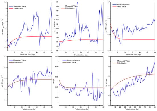
Figure 5.
Secular variation trend of the fitted values of daily ARMA models.
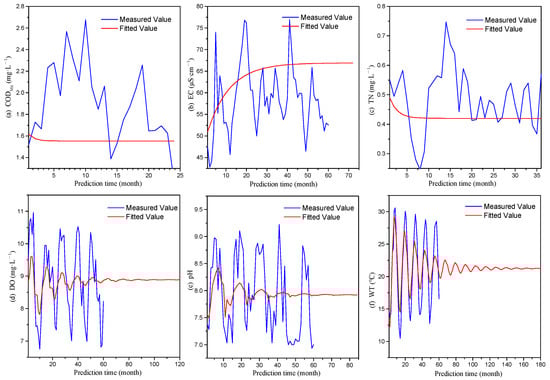
Figure 6.
Secular variation trend of the fitted values of monthly ARMA models.
To explore the mechanism behind the ARMA model’s secular trend of fitted values shown in Figure 5 and Figure 6, the lag operator in Equation (1) is expanded to obtain Equation (8).
yt = c + φ1yt−1 + φ2yt−2 + … + φpyt−p + θ1εt−1 + θ2εt−2 + … + θqεt−q + εt
The meaning of each symbol in Equation (8) is consistent with that in Equation (1). According to Equation (8), each yt can be calculated by a recursive algorithm, which allows the ARMA model to predict the future values of the time series. Under the prerequisite assumption of the ARMA model, the time series {…, yt−p, …, yt−2, yt−1, yt} must be a stationary sequence. Therefore, there must be |φj| < 1 (1 ≤ j ≤ p), |θk| < 1 (1 ≤ k ≤ q), and when t → ∞, (φ1yt−1 + φ2yt−2 + … + φpyt−p + θ1εt−1 + θ2εt−2 + … + θqεt−q + εt) → 0, yt → c, where c = μ(1 − φ1 − … − φp), μ is the mean of yt [46]. Because yt is stationary, the mean of yt does not depend on the time t. That means yt will not change with the change of t. With the continuous increase of the prediction time, c will approach a constant value, and the fitted values of an ARMA model will also approach a constant value. This is shown on the graph that the variation curve of the fitted value gradually transforms into a horizontal line.
Figure 5 and Figure 6 not only show the secular variation trend of the fitted value of the ARMA model but also reflect the change rule of the prediction error of the ARMA model from a different perspective. From Figure 5 and Figure 6, it can be seen that the difference between the fitted values and measured values is relatively small at first, and as the prediction time increases, the difference between the two becomes larger. That means the model’s prediction error also increases with the increase in prediction time because the difference between the fitted value and the measured value is the source of the prediction error. However, as the prediction time continues to increase, the fitted value gradually approaches a certain constant value. At the same time, since the time series fitted by the ARMA model are all stationary, that is, the mean value of the time series does not change with time. It means that the mean value of the time series will also approach a certain stable value. Because both the measured and fitted values all approach a certain stable value, the prediction error of the model also tends to be stabilized and no longer changes with the passage of time. This is the primary cause as to why the prediction error of the ARMA model rapidly increases in the early stage of prediction but gradually becomes stabilized as the prediction time continues to extend.
While the prediction error of the ARMA model typically stabilizes after a certain time, it also means that the fitted value remains constant after the prediction time exceeds a threshold, and the model loses its usefulness in making predictions. Therefore, the ARMA model is a short-term prediction model, and it should not be used to predict the long-term trend of time series. To reduce the prediction error, when using the ARMA model, it is recommended to limit the prediction time range as much as possible.
4.3. The Influence of Seasonal Adjustment Factors on ARMA and the Mechanism
Although the variation curve of the fitted value of the ARMA model will eventually transform into a horizontal straight line as the prediction time increases, there are differences among different ARMA models in the transformation process. All daily and monthly models’ fitted values of CODMn, EC, and TN gradually approach a constant value in a monotonic increasing or decreasing process (Figure 5 and Figure 6a–c), while the monthly models’ fitted values of DO, pH, and WT gradually approach a constant value in a process of oscillation (Figure 6d–f). The difference among them is that the three indicators of DO, pH, and WT are all introduced seasonal adjustment factors during the model construction. It can be seen that the introduction of seasonal adjustment factors will cause the fitted values of the ARMA model to exhibit some fluctuating characteristics.
The ARMA model introduced seasonal adjustment factors is called the seasonal ARMA model or SARMA model, and its expression is shown as follows:
where are the fitting parameters of the seasonal autoregressive term, are the fitting parameters of the seasonal moving average term, and S is the length of the seasonal period. and are called seasonal autoregressive term and seasonal moving average term (also known as seasonal adjustment factors).
It can be seen from Equation (8) that when the seasonal adjustment factor is introduced, the autoregressive term and the seasonal autoregressive term are multiplied, and the moving average term and the seasonal moving average term are also multiplied. For time series with obvious seasonal variation patterns, the fitted values of the ARMA model show a larger absolute peak at the integer multiple of the variation period (Figure 6d–f). Resulting in the correlation between the current value and the lag value located at the integer multiple of the seasonal period will be significantly enhanced. Therefore, the ARMA model with seasonal adjustment factors can better fit the time series with seasonal patterns and make the fitted values closer to the measured values. This is the reason why introducing the seasonal adjustment factors into the ARMA model can decrease the overall prediction error and make the growth trend of prediction errors smoother.
Seasonal adjustment factors can improve the prediction accuracy of the ARMA model to a certain extent for time series with obvious seasonal or periodic patterns. Therefore, discovering the periodic fluctuation pattern of time series as much as possible and introducing seasonal adjustment factors is an effective means to improve the prediction accuracy of the ARMA model. This is particularly important for environmental prediction because many environmental data have the characteristics of periodic changes. In practical applications, for time series with obvious seasonal fluctuations, seasonal adjustment factors can be used to reduce prediction errors directly. For the time series that are difficult to directly identify the fluctuation period, some researchers have also made some attempts. The method is to decompose the original time series into subsequences that reflect the secular variation trend and subsequences that reflect the periodic fluctuation through wavelet transform and other techniques. ARMA model is respectively constructed for each decomposed subsequence, and a seasonal adjustment factor is introduced into the model for each subsequence with periodic fluctuation. Finally, the fitted values of different subsequences are recombined to form the final prediction results [24,47].
4.4. The Contributions of the Study
The ARMA model plays a crucial role in the fields related to sustainability because sustainable research often involves the prediction and analysis of time series data, while the ARMA model is one of the most commonly used time series forecasting models. Accurate water quality forecasts are essential for environmental security and sustainability. By providing insights into future trends in water quality, the ARMA model enables utilities, resource providers, and policymakers to make informed decisions regarding environmental protection plans, resource management strategies, and sustainable infrastructure investments. This, consequently, aids in maximizing resource efficiency, cutting down the environmental footprint, and lessening the impact on the environment [48].
This study contributes by revealing the most fundamental factors affecting the forecast accuracy of the ARMA model. Through the analysis of on-site measured data and the exploration of the ARMA model’s internal mechanism, this study revealed that for the ARMA model, the prediction time is the main factor affecting the prediction error, and the sample size used for model parameters estimation is the main influencing factor for the goodness of fit. These characteristics are very important for the rational application of the ARMA model, yet they have been ignored in many studies. This study’s findings can help researchers and policymakers make more informed decisions when utilizing ARMA models to choose a more reasonable prediction time and sample size in the research and decision-making process.
4.5. Challenges and Future Prospects
The increasing levels of contamination are becoming a significant threat to water quality and the sustainability of the water system. Policymakers are facing great challenges in providing clean water sustainably by adequately addressing water systems to be free from pollutants [49]. Reliable prediction of water quality is the basis of effective water pollution control and good water environment management [8]. Water quality prediction is an important application field of the ARMA model, and it is also one of the important contributions of the ARMA model to sustainability.
Water quality change involves multiple factors, such as hydrology, chemistry, biology, and meteorology. There are complex interaction mechanisms among these factors, and a considerable part of them are nonlinear relationships. The ARMA model is essentially a linear statistical model; this makes it difficult to reflect the complex mechanisms of water quality changes and predict nonlinear change patterns. In addition, there is still a lack of in-depth research on the laws of internal correlation of time series. This leads to a lack of reliable standards for determining the sample size and prediction time in the application of ARMA models. In the future, research work should be strengthened in the following two aspects. (1) The combination of the ARMA model with other models, especially the physical models and artificial neural network models. This can improve the shortcomings of the ARMA model in long-term prediction and nonlinear prediction. (2) Explore and attempt to determine thresholds for sample size and prediction time of different types of time series, providing a reliable basis for determining sample size and prediction time of ARMA models.
5. Conclusions
In this study, a series of ARMA models were constructed based on the long-term online water quality monitoring data at the Bakou National Environment Monitoring Station of Changtan Reservoir in Zhejiang Province. Through these models, the main influencing factors of the ARMA model’s goodness of fit and prediction error were analyzed and studied. The research results show that the sample size used for model parameter estimation is the main influencing factor on the goodness of fit of the ARMA model. Within a certain range, the goodness of fit of the ARMA model increases with the increase in sample size. To build a reliable ARMA model, a certain number of samples are required for model parameter estimation. However, due to the fact that the autocorrelation between the front term and the back term in time series always decays with the increase of the interval between the front term and the back term continuously, in addition to increasing the workload of model construction and the difficulty of data collection, excessive sample size cannot further improve the goodness of fit of the ARMA model.
The prediction time is the main factor affecting the prediction error of the ARMA model, and the ARMA model is a short-term prediction model. As the prediction time increases, the correlation between the predicted value and the known value decreases, resulting in the prediction error of the ARMA model increasing continuously with the increase of prediction time. Especially during the early stages of prediction, the prediction error increases rapidly, and as the prediction time further increases, the change curve of the fitted value of the ARMA model will eventually transform into a horizontal straight line, losing the practical significance of prediction. Therefore, it is not suitable to use the ARMA model for long-term prediction research.
Introducing seasonal adjustment factors into the ARMA model for time series with periodic patterns makes the model better fit the periodic change of the time series, reduces the prediction error of the model, and achieves better prediction results.
This study reveals the most fundamental factors affecting the forecast accuracy of the ARMA model. These findings are very important for the rational application of ARMA modes. They assist researchers and policymakers in making better choices regarding the use of ARMA models selecting appropriate prediction timeframes and sample sizes for research and decision-making.
As a linear statistical model, the ARMA model is not omnipotent. In order to make up for the shortcomings of the ARMA model in long-term and nonlinear forecasting, it is necessary to strengthen the integration of the ARMA model with other models, such as physical models and artificial neural network models, in the future. The findings of this study enable environmental managers and researchers to apply the ARMA model more rationally and, hence, obtain more accurate prediction results in environmental management, sustainability, and other fields.
Author Contributions
Conceptualization, Z.L.; Data curation, C.D.; Formal analysis, J.L.; Funding acquisition, Y.C. and Y.G.; Investigation, X.L.; Methodology, Z.L.; Project administration, Y.C.; Resources, Y.W.; Supervision, Y.C.; Validation, C.D.; Visualization, C.D.; Writing—original draft, Z.L.; Writing—review and editing, Y.G. All authors have read and agreed to the published version of the manuscript.
Funding
This research was funded by The National Key Research and Development Program: Stream System Eco-logical Buffer Interception, Filtration and Purification Technology Research, grant number 2022YFC3204004; The Innovation Team Project of Nanjing Institute of Environmental Sciences, Ministry of Ecology and Environment: Characteristics of phosphorus pollution sources-sink and restoration of degraded water ecosystem in Poyang Lake, grant number ZX2023QT017; The National Natural Science Foundation of China, grant number 22206134.
Institutional Review Board Statement
Not applicable.
Informed Consent Statement
Not applicable.
Data Availability Statement
The data presented in this study are available on request from the corresponding author.
Acknowledgments
Thanks sincerely for the strong assistance provided by the Taizhou Environmental Monitoring Center in collecting water quality data from the Changtan Reservoir.
Conflicts of Interest
The authors declare no conflicts of interest.
Abbreviations
| ACF | Autocorrelation Function |
| ADF | Augmented Dickey Fuller Test |
| AI | Artificial Intelligence |
| AIC | Akaike Information Criterion |
| AR | Autoregressive Model or Autoregressive part(s) of an ARMA Model |
| ARMA | Autoregressive Moving Average Model |
| ARIMA | Autoregressive Integrated Moving Average Model |
| CODMn | Chemical Oxygen Demand for Permanganate Method |
| DO | Dissolved Oxygen |
| EC | Electrical Conductivity |
| MA | Moving Average Model or Moving Average part(s) of an ARMA Model |
| MAPE | Mean Absolute Percentage Error |
| PACF | Partial Autocorrelation Function |
| R2 | Coefficient of Determination |
| Adjusted Coefficient of Determination | |
| SARMA | Seasonal Autoregressive Moving Average Model |
| TN | Total Nitrogen |
| WT | Water Temperature |
References
- Acuña-Alonso, C.; Fernandes, A.C.P.; Álvarez, X.; Valero, E.; Pacheco, F.A.L.; Varandas, S.D.G.P.; Terêncio, D.P.S.; Fernandes, L.F.S. Water Security and Watershed Management Assessed through the Modelling of Hydrology and Ecological Integrity: A Study in the Galicia-Costa (NW Spain). Sci. Total Environ. 2021, 759, 143905. [Google Scholar] [CrossRef]
- Gupta, N.; Yadav, S.; Chaudhary, N. Time Series Analysis and Forecasting of Water Quality Parameters along Yamuna River in Delhi. Procedia Comput. Sci. 2024, 235, 3191–3206. [Google Scholar] [CrossRef]
- Ho, J.Y.; Afan, H.A.; El-Shafie, A.H.; Koting, S.B.; Mohd, N.S.; Jaafar, W.Z.B.; Lai Sai, H.; Malek, M.A.; Ahmed, A.N.; Mohtar, W.H.M.W.; et al. Towards a Time and Cost Effective Approach to Water Quality Index Class Prediction. J. Hydrol. 2019, 575, 148–165. [Google Scholar] [CrossRef]
- Hien Than, N.; Dinh Ly, C.; Van Tat, P. The Performance of Classification and Forecasting Dong Nai River Water Quality for Sustainable Water Resources Management Using Neural Network Techniques. J. Hydrol. 2021, 596, 126099. [Google Scholar] [CrossRef]
- Noori, N.; Kalin, L.; Isik, S. Water Quality Prediction Using SWAT-ANN Coupled Approach. J. Hydrol. 2020, 590, 125220. [Google Scholar] [CrossRef]
- Peng, Z.; Hu, Y.; Liu, G.; Hu, W.; Zhang, H.; Gao, R. Calibration and Quantifying Uncertainty of Daily Water Quality Forecasts for Large Lakes with a Bayesian Joint Probability Modelling Approach. Water Res. 2020, 185, 116162. [Google Scholar] [CrossRef] [PubMed]
- Wu, J.; Wang, Z. A Hybrid Model for Water Quality Prediction Based on an Artificial Neural Network, Wavelet Transform, and Long Short-Term Memory. Water 2022, 14, 610. [Google Scholar] [CrossRef]
- Jiao, G.; Chen, S.; Wang, F.; Wang, Z.; Wang, F.; Li, H.; Zhang, F.; Cai, J.; Jin, J. Water Quality Evaluation and Prediction Based on a Combined Model. Appl. Sci. 2023, 13, 1286. [Google Scholar] [CrossRef]
- Uddin, M.G.; Nash, S.; Mahammad Diganta, M.T.; Rahman, A.; Olbert, A.I. Robust Machine Learning Algorithms for Predicting Coastal Water Quality Index. J. Environ. Manag. 2022, 321, 115923. [Google Scholar] [CrossRef]
- Huang, P.; Trayler, K.; Wang, B.; Saeed, A.; Oldham, C.E.; Busch, B.; Hipsey, M.R. An Integrated Modelling System for Water Quality Forecasting in an Urban Eutrophic Estuary: The Swan-Canning Estuary Virtual Observatory. J. Mar. Syst. 2019, 199, 103218. [Google Scholar] [CrossRef]
- Zhang, Y.; Li, C.; Jiang, Y.; Sun, L.; Zhao, R.; Yan, K.; Wang, W. Accurate Prediction of Water Quality in Urban Drainage Network with Integrated EMD-LSTM Model. J. Clean. Prod. 2022, 354, 131724. [Google Scholar] [CrossRef]
- Niu, W.; Feng, Z. Evaluating the Performances of Several Artificial Intelligence Methods in Forecasting Daily Streamflow Time Series for Sustainable Water Resources Management. Sustain. Cities Soc. 2021, 64, 102562. [Google Scholar] [CrossRef]
- Peng, Z.; Hu, W.; Liu, G.; Zhang, H.; Gao, R.; Wei, W. Development and Evaluation of a Real-Time Forecasting Framework for Daily Water Quality Forecasts for Lake Chaohu to Lead Time of Six Days. Sci. Total Environ. 2019, 687, 218–231. [Google Scholar] [CrossRef] [PubMed]
- Liu, H.; Duan, Z.; Chen, C. A Hybrid Multi-Resolution Multi-Objective Ensemble Model and Its Application for Forecasting of Daily PM2.5 Concentrations. Inf. Sci. 2020, 516, 266–292. [Google Scholar] [CrossRef]
- Ebrahim Banihabib, M.; Mousavi-Mirkalaei, P. Extended Linear and Non-Linear Auto-Regressive Models for Forecasting the Urban Water Consumption of a Fast-Growing City in an Arid Region. Sustain. Cities Soc. 2019, 48, 101585. [Google Scholar] [CrossRef]
- Kow, P.Y.; Chang, L.C.; Lin, C.Y.; Chou, C.C.; Chang, F.J. Deep Neural Networks for Spatiotemporal PM2.5 Forecasts Based on Atmospheric Chemical Transport Model Output and Monitoring Data. Environ. Pollut. 2022, 306, 119348. [Google Scholar] [CrossRef]
- Veerendra, G.T.N.; Kumaravel, B.; Rao, P.K.R.; Dey, S.; Manoj, A.V.P. Forecasting Models for Surface Water Quality Using Predictive Analytics. Environ. Dev. Sustain. 2024, 26, 15931–15951. [Google Scholar] [CrossRef]
- Niknam, A.R.R.; Sabaghzadeh, M.; Barzkar, A.; Shishebori, D. Comparing ARIMA and Various Deep Learning Models for Long-Term Water Quality Index Forecasting in Dez River, Iran. Environ. Sci. Pollut. Res. 2024. [Google Scholar] [CrossRef]
- Li, N.; Li, Y.; Feng, J.; Shan, Y.; Qian, J. Construction and application optimization of the chl-a forecast model ARIMA for lake Taihu. Environ. Sci. 2021, 42, 2223–2231. [Google Scholar]
- Cipra, T. Time Series in Economics and Finance; Springer Nature: Cham, Switzerland, 2020; pp. 123–174. [Google Scholar] [CrossRef]
- Gibrilla, A.; Anornu, G.; Adomako, D. Trend Analysis and ARIMA Modelling of Recent Groundwater Levels in the White Volta River Basin of Ghana. Groundw. Sustain. Dev. 2018, 6, 150–163. [Google Scholar] [CrossRef]
- Yan, B.; Mu, R.; Guo, J.; Liu, Y.; Tang, J.; Wang, H. Flood Risk Analysis of Reservoirs Based on Full-Series ARIMA Model under Climate Change. J. Hydrol. 2022, 610, 127979. [Google Scholar] [CrossRef]
- Valipour, M.; Banihabib, M.E.; Behbahani, S.M.R. Comparison of the ARMA, ARIMA, and the Autoregressive Artificial Neural Network Models in Forecasting the Monthly Inflow of Dez Dam Reservoir. J. Hydrol. 2013, 476, 433–441. [Google Scholar] [CrossRef]
- Khan, M.M.H.; Muhammad, N.S.; El-Shafie, A. Wavelet Based Hybrid ANN-ARIMA Models for Meteorological Drought Forecasting. J. Hydrol. 2020, 590, 125380. [Google Scholar] [CrossRef]
- Narayanan, P.; Basistha, A.; Sarkar, S.; Kamna, S. Trend Analysis and ARIMA Modelling of Pre-Monsoon Rainfall Data for Western India. Comptes Rendus Géoscience 2013, 345, 22–27. [Google Scholar] [CrossRef]
- Nury, A.H.; Hasan, K.; Alam, M.J.B. Comparative Study of Wavelet-ARIMA and Wavelet-ANN Models for Temperature Time Series Data in Northeastern Bangladesh. J. King Saud Univ. Sci. 2017, 29, 47–61. [Google Scholar] [CrossRef]
- Qin, M.; Li, Z.; Du, Z. Red Tide Time Series Forecasting by Combining ARIMA and Deep Belief Network. Knowl.-Based Syst. 2017, 125, 39–52. [Google Scholar] [CrossRef]
- Lotfi, K.; Bonakdari, H.; Ebtehaj, I.; Mjalli, F.S.; Zeynoddin, M.; Delatolla, R.; Gharabaghi, B. Predicting Wastewater Treatment Plant Quality Parameters Using a Novel Hybrid Linear-Nonlinear Methodology. J. Environ. Manag. 2019, 240, 463–474. [Google Scholar] [CrossRef]
- Huang, J.; Qian, J.; Yin, H. Application of ARIMA model in forecasting total phosphorus of Suzhou Creek. Chin. J. Environ. Eng. 2007, 1, 139–143. [Google Scholar]
- Li, Y.; Han, T.; Wang, J.; Quan, W.; He, D.; Jiao, R.; Wu, J.; Guo, H.; Ma, Z. Application of ARIMA Model for Mid- and Long-term Forecasting of Ozone Concentration. Environ. Sci. 2021, 42, 3118–3126. [Google Scholar] [CrossRef]
- Cao, L.; Liu, H.; Li, J.; Yin, X.; Duan, Y.; Wang, J. Relationship of Meteorological Factors and Human Brucellosis in Hebei Province, China. Sci. Total Environ. 2020, 703, 135491. [Google Scholar] [CrossRef] [PubMed]
- Nickerson, D.M.; Madsen, B.C. Nonlinear Regression and ARIMA Models for Precipitation Chemistry in East Central Florida from 1978 to 1997. Environ. Pollut. 2005, 135, 371–379. [Google Scholar] [CrossRef] [PubMed]
- Pektaş, A.O.; Kerem Cigizoglu, H. ANN Hybrid Model versus ARIMA and ARIMAX Models of Runoff Coefficient. J. Hydrol. 2013, 500, 21–36. [Google Scholar] [CrossRef]
- Mandal, A.; Biswas, J.; Farooqui, Z.; Roychowdhury, S. A Detailed Perspective of Marine Emissions and Their Environmental Impact in a Representative Indian Port. Atmos. Pollut. Res. 2021, 12, 101194. [Google Scholar] [CrossRef]
- Zhang, L.; Lin, J.; Qiu, R.; Hu, X.; Zhang, H.; Chen, Q.; Tan, H.; Lin, D.; Wang, J. Trend Analysis and Forecast of PM2.5 in Fuzhou, China Using the ARIMA Model. Ecol. Indic. 2018, 95, 702–710. [Google Scholar] [CrossRef]
- JI, C.; Hou, D.; Xie, L.; Sun, H.; Li, F.; Zhou, Y.; Deng, A.; Shen, H.; Bao, G.; Wang, Y. Analysis and Prediction of Health Risk from Heavy Metals in Drinking Water Sources Based on Time Series Model. Environ. Sci. 2021, 42, 5322–5332. [Google Scholar]
- Cheng, Y.; Zhang, H.; Liu, Z.; Chen, L.; Wang, P. Hybrid Algorithm for Short-Term Forecasting of PM2.5 in China. Atmos. Environ. 2019, 200, 264–279. [Google Scholar] [CrossRef]
- Liu, Y.; Luo, H.; Xie, T. Research and application of PM2.5 concentration prediction model based on XGBoost-ARIMA method. J. Saf. Environ. 2023, 23, 211–221. [Google Scholar] [CrossRef]
- Sheikhy Narany, T.; Aris, A.Z.; Sefie, A.; Keesstra, S. Detecting and Predicting the Impact of Land Use Changes on Groundwater Quality, a Case Study in Northern Kelantan, Malaysia. Sci. Total Environ. 2017, 599–600, 844–853. [Google Scholar] [CrossRef]
- Liu, C.; Yang, L.; Deng, H.; Guo, Y.; Li, D.; Duan, Q. Prediction of ammonia concentration in piggery based on ARIMA and BP neural network. Environ. Sci. 2019, 39, 2320–2327. [Google Scholar] [CrossRef]
- Phan, T.-T.-H.; Nguyen, X.H. Combining Statistical Machine Learning Models with ARIMA for Water Level Forecasting: The Case of the Red River. Adv. Water Resour. 2020, 142, 103656. [Google Scholar] [CrossRef]
- Wang, P.; Zhang, H.; Qin, Z.; Zhang, G. A Novel Hybrid-Garch Model Based on ARIMA and SVM for PM2.5 Concentrations Forecasting. Atmos. Pollut. Res. 2017, 8, 850–860. [Google Scholar] [CrossRef]
- Sun, Z.; Li, Y.; Yu, J.; Wang, F. Eeosystem service evaluation of the six important reservoirs in Zhejiang Province. J. Zhejiang Univ. Sci. Ed. 2015, 42, 353–364. [Google Scholar]
- Hamilton, J.D. Time Series Analysis; Xia, X., Translator; China Renmin University Press: Beijing, China, 2014; pp. 49–80. [Google Scholar]
- Zhang, X. Econometrics, 4th ed.; Nankai University Press: Tianjin, China, 2014; pp. 261–289. [Google Scholar]
- Shumway, R.H.; Stoffer, D.S. Time Series Analysis and Its Applications: With R Examples, 4th ed.; Springer Texts in Statistics; Springer International Publishing: Cham, Switzerland, 2017; pp. 75–88. [Google Scholar]
- Aladağ, E. Forecasting of Particulate Matter with a Hybrid ARIMA Model Based on Wavelet Transformation and Seasonal Adjustment. Urban Clim. 2021, 39, 100930. [Google Scholar] [CrossRef]
- Durmus Senyapar, H.N.; Aksoz, A. Empowering Sustainability: A Consumer-Centric Analysis Based on Advanced Electricity Consumption Predictions. Sustainability 2024, 16, 2958. [Google Scholar] [CrossRef]
- Dawood, T.; Elwakil, E.; Novoa, H.M.; Gárate Delgado, J.F. Toward Urban Sustainability and Clean Potable Water: Prediction of Water Quality via Artificial Neural Networks. J. Clean. Prod. 2021, 291, 125266. [Google Scholar] [CrossRef]
Disclaimer/Publisher’s Note: The statements, opinions and data contained in all publications are solely those of the individual author(s) and contributor(s) and not of MDPI and/or the editor(s). MDPI and/or the editor(s) disclaim responsibility for any injury to people or property resulting from any ideas, methods, instructions or products referred to in the content. |
© 2024 by the authors. Licensee MDPI, Basel, Switzerland. This article is an open access article distributed under the terms and conditions of the Creative Commons Attribution (CC BY) license (https://creativecommons.org/licenses/by/4.0/).