Spatial Interaction Spillover Effect of Tourism Eco-Efficiency and Economic Development

Abstract

Tourism eco-efficiency (TEE) is a pivotal metric for assessing tourism’s sustainability and the balance between human activities and the environment, significantly influencing regional economic growth (RGDP). This research utilizes a comprehensive analytical framework, combining the Super SBM-DEA model, the Malmquist index, and spatial econometric models, to analyze the spatial interplay between TEE and RGDP within the Yangtze River Economic Belt (YREB) from 2009 to 2021. The results show that (1) TEE in the YREB exhibits a generally upward trajectory with fluctuations, with upstream and downstream regions consistently outperforming the midstream areas in terms of efficiency; (2) technological progress is identified as the primary driver behind efficiency variations; (3) and there exists a symbiotic relationship between local TEE and RGDP, where the economic prosperity of adjacent regions exerts a competitive pull on local TEE, while the TEE of neighboring areas can slow down local economic growth. The study concludes with strategic recommendations aimed at fostering regional collaborative advancement, offering valuable insights for the sustainable development agenda of nations and regions.

1. Introduction

With the deepening of economic globalization, the tourism industry has become one of the fastest-growing sectors in the global economy, and the comprehensive contribution rate to the socio-economic system has exceeded 10% [1]. The tourism industry should ideally be a domain that practices the concept of low carbon emissions [2]. However, with the continuous rise in consumer spending, the booming development of the tourism industry has also led to a series of issues, including ecological destruction and greenhouse gas emissions [3]. According to research, the carbon emissions from tourism account for 8.3% of the global carbon emissions [4]. Striking a balance between tourism revenue and the environmental costs of tourism is crucial for the sustainable development of the tourism industry.

Tourism eco-efficiency (TEE) is a tool used to measure the level of tourism colocalization and its sustainable development, and it has garnered widespread attention in the academic community. By improving TEE, it is possible to achieve economic growth while minimizing environmental damage [5]. However, in the measurement of TEE, existing studies, on the one hand, have neglected the non-desired output of ecological costs, leading to an overestimation of efficiency values; on the other hand, the efficiency values calculated are static, making it challenging to reflect the relative changes in efficiency values across periods and the reasons for these changes. Furthermore, although many scholars have identified the level of economic development as a key factor affecting TEE, in today’s rapidly developing context of informatization, technological advancement, and the internet, regional cooperation and competition are becoming increasingly fierce. The relationship between TEE and RGDP is also intricate. It is insufficient to only study the unidirectional impact of RGDP on TEE.

Responding to the above research gaps, this study aims to delineate the bidirectional interaction between TEE and economic development, offering guidance for policymakers to foster sustainable growth. Taking the Yangtze River Economic Belt (YREB) as a case study, this paper employs the super SBM-DEA model and the Malmquist index model to measure TEE. The methodology not only accounts for undesirable outputs for more accurate efficiency measures but also analyzes the dynamic changes in TEE and identifies the factors driving these changes. Ultimately, a spatial econometric model is utilized to empirically examine the relationship between TEE and economic development.

Our research makes two key contributions. Primarily, this paper advances the measurement of TEE by incorporating the analysis of undesirable outputs that arise from the tourism development process. This approach not only unveils the dynamics of TEE but also dissects the underlying factors driving its fluctuations. Concurrently, this study delineates and quantifies the intricate bidirectional interplay between TEE and RGDP. The findings are not confined to the context of the study; they are extrapolatable to other regions within China and apply to a broader spectrum of countries and territories.

This paper is structured in the following manner. Section 2 presents a literature review and hypothesis. Section 3 presents the methodology. Section 4 presents the study of the empirical results. Section 5 organizes further discussion. Finally, Section 6 reports the conclusions and suggestions.

2. Literature Review and Hypothesis

2.1. Tourism Eco-Efficiency

TEE, as an application of eco-efficiency research in the tourism industry, serves both as an objective assessment of the ecological level of the tourism industry and as an essential tool for measuring the sustainable development of the tourism industry [6]. Currently, academic research on TEE mainly focuses on measurement methods [7,8,9] and driving factors [10,11]. Gössling (2005) posits that the essence of TEE lies in calculating the CO₂ emissions per unit of tourism economic output, which can be used to evaluate the environmental impact and sustainability of the tourism industry [12]. Various methods can be used to measure TEE, including the single ratio method [8], ecological footprint method [13], carbon footprint method [14], input–output analysis method [15], and the widely applied Data Envelopment Analysis (DEA) model [16,17]. Kytzia (2011) employed the model method in studying the eco-efficiency of land use in the tourism industry [18]. Tsionas et al. (2014) reviewed the literature on the efficiency of tourist destinations and found that most of them used the DEA method [19]. However, these measurements are all static TEE assessments, which fail to reflect the changes in TEE and the reasons for these changes. Moreover, they only consider the desired outputs, neglecting the non-desired outputs, leading to an overestimation of efficiency measures and affecting the accuracy of TEE research. Consequently, scholars have gradually optimized the measurement methods to account for the environmental costs of non-desired outputs. Carboni et al. (2018) applied the Data Envelopment Analysis and Malmquist productivity index to measure the environmental efficiency and economic efficiency of 20 regions in Italy from 2004 to 2011 [20]. However, there is a scarcity of research applying these methods to measure the ecological efficiency of the tourism industry. Therefore, to reduce the measurement error of TEE and dynamically reflect its changes, this paper comprehensively applies the super SBM-DEA model based on non-desired outputs and the Malmquist index model to measure TEE.

2.2. Tourism Eco-Efficiency and Regional Economic Development

In the study of the correlation between TEE and RGDP, scholars have emphasized the significant impact of economic development on TEE [10,21,22]. Jiang et al. (2021) found that the level of economic development, degree of openness, professionalism in tourism, and transportation conditions can significantly enhance tourism efficiency [23]; some researchers have concluded that the level of economic development, technological progress, and urbanization are key factors influencing TEE [10,22]. In addition, some scholars have explored the interactive response relationship between tourism’s ecological benefits and tourism for economic development [24,25]. As a strategic pillar industry, the development of the tourism industry has a positive impact on local employment and economic growth [26]. TEE is again a tool for measuring the degree of sustainable development of the tourism industry and may also impact economic development. However, in the existing literature, most attention is paid on the unidirectional relationship between RGDP and TEE, and there is insufficient discussion on whether there is an interactive relationship between the two and the mechanism of their interactive influence. Specifically, the theoretical analysis and hypotheses of this paper are as follows.

2.2.1. Positive Impact of RGDP on TEE

The promotional effect of RGDP on TEE is manifested in two main aspects. The first aspect is market diversification and benefit perception: The diversification of the regional economy contributes to reducing the tourism industry’s reliance on a single market, enhancing the industry’s resilience to market risks and fostering its development. This, in turn, promotes the improvement of (TEE) [26]. Additionally, as the tourism industry develops, it increases local residents’ income and enhances their quality of life. Based on the economic benefit perception, community members perceive tourism as beneficial to the local economy, thereby increasing their involvement in tourism planning, decision-making, and activities [27]. Consequently, the enhancement of residents’ economic capabilities motivates greater support for the development of the local tourism industry, with community members participating as tourists or tourism professionals, contributing to the development of the industry and consequently enhancing TEE.

The second aspect is infrastructure and public services: The investment capacity of the regional economy determines the completeness of local tourism infrastructure and service systems. The establishment of infrastructure such as transportation, accommodation, and tourism information services not only improves the accessibility of tourist destinations but also enhances the quality of the visitor experience, attracting more tourism consumption and promoting the growth of tourism revenue, thereby enhancing TEE. Furthermore, according to Porter’s cluster theory, robust infrastructure is a critical factor in the development of tourism industry clusters [28]. Tourism industry clusters significantly enhance tourism competitiveness and have a pronounced positive effect on the industry’s development [29]. Therefore, areas with robust economic development possess more sophisticated infrastructure and superior public services, fostering tourism industry clusters and enhancing the industry’s competitiveness, thus further elevating TEE. This hypothesis is proposed based on the analysis that RGDP has a positive effect on TEE.

2.2.2. Positive Impact of TEE on RGDP

The promotional effect of TEE on RGDP manifests itself in three main aspects. The first aspect is job creation. As an essential service industry component, tourism has a direct and indirect driving effect on RGDP. The sustained development of the tourism industry will increase tourism revenue, thereby promoting economic growth.. Meanwhile, the tourism industry has intense labor characteristics, which can provide employment opportunities for residents, reduce unemployment rates, and promote economic growth [27]. The higher the TEE, the more obvious its promotional effect on RGDP. The second aspect is foreign exchange income and the balance of payment equilibrium. As an important part of the service trade, the tourism industry can bring foreign exchange income to the regional economy, increase foreign exchange reserves, and improve the balance of payments. Especially in developing countries, foreign exchange income from the tourism industry plays a key role in balancing the balance of payments and stabilizing the exchange rate [30]. The third focus is on achieving regional development equilibrium and enhancing social welfare. The tourism industry’s continuous development helps promote the balanced development of the regional economy. In addition, the constant development of the tourism industry can also improve the quality of life for residents, enhance social welfare by providing leisure and entertainment facilities, and improve infrastructure.

This hypothesis is proposed based on the analysis that TEE has a positive effect on RGDP.

2.2.3. The Interaction between TEE and RGDP

The spatial interactive mechanism between TEE and RGDP is complex. Luo et al. (2022) found that the main impact of economic development on tourism ecological efficiency lies in the allocation of resources such as human and capital [31]. The research object of this article spans across the eastern, central, and western regions of China, with significant regional development disparities [31]. When neighboring areas experience rapid economic growth, it may attract resources such as capital, technology, and talent to flow out. This loss of resources may affect the sustainable development of the local tourism industry, thereby suppressing the improvement of TEE. In addition, economic growth in neighboring areas may bring environmental pressure, and ecological issues can harm the attractiveness of the local tourism industry, thereby affecting TEE. On the other hand, improving the TEE in neighboring areas has a siphoning effect on local economic growth. The improvement of the TEE in neighboring areas means that these areas perform well in utilizing tourism resources and environmental protection, which may attract more tourists and investments, thus siphoning the local tourism market and economic growth. Neighboring areas with high TEE may offer more competitive tourism products and services, attracting tourism consumption that might have flowed to the local area, leading to a slowdown in local tourism revenue and the growth of related industries.

This hypothesis is proposed based on the analysis conducted. The economic growth of neighboring areas has a siphoning effect on local TEE, and the improvement of neighboring TEE has an inhibitory effect on the local RGDP.

Based on this analysis, this paper proposes a theoretical framework, as shown in Figure 1.

3. Methodology

3.1. Study Area

The Yangtze River Economic Belt (YREB), spanning vast geographical regions across China, harbors a significant population base and robust economic aggregate. In 2021, the collective GDP of the 11 provinces and cities within the YREB totaled CNY 53,022.78 billion, comprising a substantial 46.14% of the national GDP. Notably, the tertiary industry accounted for 53.63% of the regional economic output, emphasizing its pivotal role in the YREB. Additionally, the YREB is a repository of tourism resources, attracting visitors from both domestic and international markets. According to the “Statistical Yearbook of Chinese Culture, Heritage, and Tourism 2022”, the YREB holds a substantial share of starred hotels (42.14%) and A-level scenic spots (39.55%) of the national total. Notably, in 2021, the YREB welcomed 66.34% of the national total tourists. As such, the YREB assumes a pivotal role in spearheading the transition to a low-carbon economy and advancing high-quality economic development in China [32]. Historically, the region has heavily relied on high input and resource consumption to drive economic development, consequently resulting in significant ecological pressures, particularly air and water pollution, which pose considerable challenges to environmental health and sustainable development [33]. Therefore, fostering the development and transformation of green industries, especially tourism, is crucial for achieving sustainability in this region. This necessitates a comprehensive reassessment of the intricate interactions and spillover effects between economic growth and sustainable tourism practices within the YREB. Based on the “Guiding Opinions of the State Council on Promoting the Development of the Yangtze River Economic Belt Relying on the Golden Waterway”, the YREB is geographically classified into the upstream region (Chongqing, Sichuan, Yunnan, Guizhou), the midstream region (Hubei, Hunan, Jiangxi), and downstream (Shanghai, Jiangsu, Zhejiang, Anhui) region [34]. This study establishes a corresponding regional division to facilitate further in-depth research (Figure 2).

3.2. Index System and Variables

3.2.1. Index System

The core of TEE lies in maximizing output with minimal resource input during the evolution of the tourism industry, thus serving as a potent metric for assessing the sustainability of regional tourism [7]. Consequently, the development of a scientific evaluation index system is paramount in reflecting the TEE of the YREB. Drawing on the frameworks established by Liu et al. (2017) [11] and Ruan et al. (2019) [13] and taking into account data availability, this study formulates an evaluation index for the TEE of the YREB, encompassing both input and output considerations (

Table 1. Input–output index system of TEE.

Type	Level 1	Level 2	Unit
Input indicators	capital investment	number of 3A and above tourist attractions	number
		number of 3-star and above hotels	number
		number of travel agencies	number
Output indicators	expected outputs	earnings from domestic tourism	10,000 RMB
		foreign exchange earnings from international tourism	10,000 USD
	unexpected outputs	carbon emissions from the tourism industry	10,000 tons

).

Input Indicators: Given the resource-intensive nature of tourism development, this paper, building upon previous research [13,35], identifies key input indicators that encompass resources, infrastructure, and land utilization. Specifically, we select the number of 3A and above tourist attractions, three-star hotels, and travel agencies as proxies for capital investment in the tourism sector.

Output Indicators: ① Desired Outputs: To assess the economic benefits of tourism, this paper utilizes the total tourism revenue as the primary metric. The total tourism revenue is calculated as the aggregate of domestic tourism revenue and tourism foreign exchange income, adjusted for the year’s average exchange rate. ② Undesirable Outputs: This study measures the environmental impact of tourism, focusing on carbon emissions. Drawing from existing studies [33,36], we estimate carbon emissions from three primary sources: tourism transportation, tourism accommodation, and tourism activities.

3.2.2. Variables

This study employs panel data spanning from 2009 to 2021, encompassing 11 provinces and cities within the YREB as the analytical sample (

Table 2. Variable summary.

Variable Type	Variable Name	Indicator Description	Abbreviation
Core variables	Tourism eco-efficiency	Obtained through the calculation in this study	TEE
	Regional economic development	Regional Gross Domestic Product (10,000 RMB)	RGDP
Control variables	Visitor scale	Total number of tourists (10,000 person-times)	vissca
	Scale of the tourism economy	Total tourism incomes (10,000 RMB)	toureco
	Structure of the tourism industry	Total tourism incomes/GDP of the tertiary sector	tourindustr
	The level technological innovation	The number of granted patents (piece)	scitech
	Urbanization level	The urbanization rate	urb
	Industrial structure	GDP of the tertiary sector/GDP	industr

). The pertinent indicators are explained as follows:

Core variables: The core variables of this study are TEE and RGDP. Precisely, TEE is measured by the super SBM-DEA model and the Malmquist index model; RGDP is represented by the Gross Regional Product (GRP).

Control Variables: This study’s simultaneous equation model incorporates six control variables [4,11,37,38]. Specifically, four variables—tourist scale, tourism economic scale, tourism industry structure, and technological innovation level—comprise the control variable group X in the tourism equation. In the regional economic equation, three variables—urbanization level, industrial structure, and technological innovation level—constitute the control variable group Y. Below is a brief explanation of these control variables:

Tourist scale: The influx of tourists generates revenue but also poses environmental challenges affecting the sustainable development of local ecology and tourism [11].

Tourism economic scale: Lenzen’s study indicates an inverse “U” relationship between the TEE and tourism economic scale. Initially, as tourism revenue grows, TEE improves; however, it declines once a certain threshold is reached [4]. Consequently, this paper includes the total tourism revenue as a control variable.

Tourism industry structure: Research suggests that optimizing the industrial structure enhances TEE [37]. A rational structure accelerates industrial agglomeration, realizes economies of scale, and reduces environmental stress, thereby improving TEE. This paper measures it as the proportion of the total tourism revenue to the tertiary industry’s output value.

Level of technological innovation: Studies show that scientific and technological innovation drives sustainable economic and tourism development, increasing TEE’s value [37]. With a fixed tourism revenue, higher technological advancement leads to lower energy consumption and environmental pollution. This paper represents it through the number of patent applications and authorizations.

Urbanization level: Urbanization fosters regional economic growth by optimizing industrial structure and resource allocation [39]. This paper measures it as the urban population proportion. Additionally, the proportion of the tertiary sector in GDP reflects industrial structure optimization, which is expected to foster economic growth and sustainability.

Descriptive statistics of related variables have been placed in Appendix A.

3.3. Data Sources

Given the availability of data, the research period for this study is confined to the years spanning 2009 to 2021.

Core Variables: The data for the three input indicators of tourism ecological efficiency were derived from the China Yearbook of Cultural Relics and Tourism Statistics (2010–2022). Among them, the data for the desired output indicators originate from the statistical yearbooks of 11 provinces and cities (2010–2022), while the non-desired output indicators were calculated accordingly.

Control Variables: The data for tourism-related indicators were also obtained from the China Yearbook of Cultural Relics and Tourism Statistics (2010–2022). As for other indicators, they were sourced from various statistical yearbooks, including the Shanghai Statistical Yearbook (2010–2022), Anhui Statistical Yearbook (2010–2022), Jiangsu Statistical Yearbook (2010–2022), Zhejiang Statistical Yearbook (2001–2020), Sichuan Statistical Yearbook (2001–2020), Jiangxi Statistical Yearbook (2001–2020), Hunan Statistical Yearbook (2001–2020), Hubei Statistical Yearbook (2001–2020), Chongqing Statistical Yearbook (2001–2020), Guizhou Statistical Yearbook (2001–2020), and Yunnan Statistical Yearbook (2001–2020).

3.4. Methods

3.4.1. The Super SBM-DEA Model

This paper employs an enhanced SBM-DEA model that considers both desired and undesired outputs to measure the TEE of the 11 provinces and cities along the YREB. The model is constructed as follows:

$$\mathsf{\rho }=\mathrm{M}\mathrm{i}\mathrm{n}{\displaystyle \frac{\frac{1}{m}\sum _{i=1}^m\left(\frac{\overline{x}}{x_{i}k}\right)}{\frac{1}{r_1+r_2}\left(\sum _{s=1}^{r_1}\frac{\overline{y^d}}{y_{sk}^d}+\sum _{q=1}^{r_2}\frac{\overline{y^u}}{y_{qk}^u}\right)}}$$

(1)

$$\overline{x}\ge \sum _{j=1,\ne k}^n{x}_{ij}{\lambda }_j;\overline{y^d}\le \sum _{j=1,\ne k}^n{y}_{sj}^d{\lambda }_j;\overline{y^d}\ge \sum _{j=1,\ne k}^n{y}_{qj}^d{\lambda }_j$$

(2)

$$\overline{x}\ge xk;\overline{y^d}\le y_k^d;\overline{y^u}\ge y_k^u;$$

(3)

$${\lambda }_j\ge 0,i=\mathrm{1,2}\dots ,m$$

(4)

$$\mathrm{j}=\mathrm{1,2},\dots ,n_j=\mathrm{1,2},\dots , nq=\mathrm{1,2},\dots ,r_2$$

(5)

In Equations (1) and (2), $n$ DMUs are considered, with each DMU consisting of m inputs, desired outputs $r_1$, and undesired outputs $r_2$. The elements within the input matrix, desired output matrix, and undesired output matrix are denoted by $x$, $y^d,\mathrm{a}\mathrm{n}\mathrm{d}{ y}^u$, respectively. d and u represent the desired output and undesired output, respectively. $\mathsf{\rho }$ represents the value of TEE.

3.4.2. The Malmquist Model

The Malmquist model not only overcomes the limitation of traditional DEA models, which can only reflect static efficiency by providing a dynamic perspective on efficiency information, but it also enables the decomposition of efficiency into two distinct components: technical efficiency and technological progress. Furthermore, it allows for the additional breakdown of technical efficiency into pure technical efficiency and scale efficiency, thereby facilitating a more in-depth analysis of efficiency. Therefore, this paper employs the Malmquist model to address the gap in existing research that lacks a thorough analysis of the dynamic changes in tourism ecological efficiency and their causes. Since the Malmquist model requires various outputs to change in the same direction, it is not suitable to treat unexpected outputs as negative outputs. This article draws on the method of Cheng (2021) [40] and treats unexpected outputs as input indicators, which can directly use the Malmquist model. The formula is as follows:

$$\mathrm{T}\mathrm{f}\mathrm{p}\mathrm{c}\mathrm{h}=\mathrm{E}\mathrm{f}\mathrm{f}\mathrm{c}\mathrm{h}\times \mathrm{T}\mathrm{e}\mathrm{c}\mathrm{h}\mathrm{c}\mathrm{h}=(\mathrm{P}\mathrm{e}\mathrm{c}\mathrm{h}\times \mathrm{S}\mathrm{e}\mathrm{c}\mathrm{h})\times \mathrm{T}\mathrm{e}\mathrm{c}\mathrm{h}\mathrm{c}\mathrm{h}$$

(6)

$$\mathrm{E}\mathrm{f}\mathrm{f}\mathrm{c}\mathrm{h}={\displaystyle \frac{D_0^t\left(x_{t+1},y_{t+1}\right)}{D_0^t\left(x_t,y_t\right)}}$$

(7)

$$\mathrm{T}\mathrm{e}\mathrm{c}\mathrm{h}\mathrm{c}\mathrm{h}={\left[{\displaystyle \frac{D_0^t\left(x_{t+1},y_{t+1}\right)}{D_0^{t+1}\left(x_{t+1},y_{t+1}\right)}}\times {\displaystyle \frac{D_0^t\left(x_t,y_t\right)}{D_0^t\left(x_t,y_t\right)}}\right]}^{{\displaystyle \raisebox{1ex}{$1$}\!\left/ \!\raisebox{-1ex}{$2$}\right.}}$$

(8)

Usually, it is compared with the value of 1 to evaluate changes in efficiency (increase, decrease, and stability). If Tfpch > 1, then the efficiency in period t + 1 has improved compared to period t; if Tfpch < 1, then the efficiency in period t + 1 has declined compared to period t; if Tfpch = 1, then the efficiency in period t + 1 is consistent with that of period t.

Similarly, Tfpch, Techch, Pech, and Sech values greater than 1 indicate an increase in TEE, technological progress, pure technical efficiency, and economies of scale from period t to t + 1, respectively. Conversely, values less than 1 suggest a decrease in TEE, technological stagnation, deterioration in pure technical efficiency, and diseconomies of scale.

3.4.3. The Spatial Simultaneous Equation Model

The literature review shows that a complex interrelationship exists between TEE and RGDP, which may be subject to spatial spillover effects. Utilizing the traditional single-equation spatial Durbin model may overlook the endogeneity issues among core variables, and it cannot test the interrelationships between variables, whereas employing a panel model that does not account for spatial spillover effects could lead to the loss of such effects. Consequently, when constructing a theoretical model for interactive relationships, it is necessary to incorporate spatial factors. The Generalized Spatial Three-Stage Least Squares (GS3SLS) method not only considers the spatial interaction and spillover effects but also effectively addresses the endogeneity issues between core variables. Scholars have applied this method in studying related matters and have obtained robust estimation results [41]. Therefore, this paper constructs a spatial econometric panel data model and employs the GS3SLS method for estimation.

(1)

Model Specification

The spatial econometric system of equations established in this paper to examine the interactive relationship between TEE and RGDP is as follows:

$${TEE}_{it}={\alpha }_0+{\alpha }_{1}W{TEE}_{it}+{\alpha }_2{RGDP}_{it}+{\alpha }_{3}W{RGDP}_{it}+\lambda X+{\mathsf{\eta }}_i$$

(9)

$${RGDP}_{it}={\beta }_0+{{\beta }_{1}W{RGDP}_{it}+\beta }_2{TEE}_{it}+{\beta }_{3}W{TEE}_{it}+\rho Y+{\mu }_i$$

(10)

In Equations (9) and (10), $i$ denotes the region, and $t$ denotes the year. ${TEE}_{it}$ represents the TEE values for various provinces and cities in different years, while ${RGDP}_{it}$ represents the economic development levels for various provinces and cities in different years. X signifies the control variables that affect TEE; Y signifies the control variables that influence the regional economic development level. W is the spatial weight matrix; ${ℇ}_{it} \mathrm{a}\mathrm{n}\mathrm{d} {\xi }_{it}$ are the stochastic error terms. ${\alpha }_0 \mathrm{a}\mathrm{n}\mathrm{d} {\beta }_0 \mathrm{a}\mathrm{r}\mathrm{e} \mathrm{t}\mathrm{h}\mathrm{e} \mathrm{c}\mathrm{o}\mathrm{n}\mathrm{s}\mathrm{t}\mathrm{a}\mathrm{n}\mathrm{t} \mathrm{t}\mathrm{e}\mathrm{r}\mathrm{m}\mathrm{s}, \mathrm{a}\mathrm{n}\mathrm{d} {\alpha }_1$ is the coefficient for the spatial spillover effect of TEE, indicating the extent to which the sustainable development of tourism in neighboring regions affects the local tourism industry development; ${\beta }_1$ is the coefficient for the spatial spillover effect of RGDP, indicating how the economic development level in neighboring regions affects the local economic development. ${\alpha }_2$ and ${\beta }_2$ are used to represent the interactive effect between regional economic development and TEE, that is, ${\alpha }_2$ and ${\beta }_2$ quantitatively reflect the degree of interaction between RGDP and TEE. ${\alpha }_3$ and ${\beta }_3$ are used to represent the spillover effect between regional economic development and TEE, that is, ${\alpha }_3$ and ${\beta }_3$ quantitatively represent the degree of spatial spillover between RGDP and TEE.

(2)

Setting of the spatial weight matrix

According to the new economic geography theory, at different stages, the interactive status between two regions is unequal and highly correlated with their levels of economic development. Therefore, based on the research of Li et al. (2017), this paper establishes an economic geography-based weighting that more accurately measures the spatial spillover effects between regions [42]. The spatial weight matrix is rigorously formulated utilizing an asymmetric geographical economic distance matrix to ensure academic precision and conciseness [42], which satisfies the following formula:

$$W_1=w_{ij}^E=w_{ij}^{G}diag\left({\displaystyle \frac{P{Y}_1}{PY}},{\displaystyle \frac{P{Y}_2}{PY}},\dots \dots ,{\displaystyle \frac{P{Y}_n}{PY}}\right)$$

(11)

$$w_{ij}^G=1/d_{ij}^2$$

(12)

$$P{Y}_i={\displaystyle \frac{1}{{(t}_1-t_0+1)\sum _{t_0}^{t_1}{Y}_{it}}}$$

(13)

$$PY={\displaystyle \frac{1/n}{(t_1-t_0+1)\sum _1^n\sum _{t_0}^{t_1}{Y}_{it}}}$$

(14)

In Equations (11)–(14), d_ij represents the shortest distance between the economies of each province and city, and this article calculates it using the Euclidean distance of the provincial capital city. $w_{ij}^G$ denotes the economic geography weight matrix, $P{Y}_i$ is the average actual per capita GDP for region I, and PY is the average actual per capita GDP across the sample cities, with the variables subsequently being standardized.

4. Results

4.1. Measurement and Decomposition

4.1.1. Super SBM-DEA Model Measurements

This paper adopts a non-oriented undesirable output super SBM-DEA model, focusing on the input perspective and assuming constant returns to scale, to quantify the tourism ecological efficiency (TEE) of 11 provinces and cities in the YREB from 2009 to 2021. The findings are summarized in

Table 3. TEE in the YREB, 2009–2021.

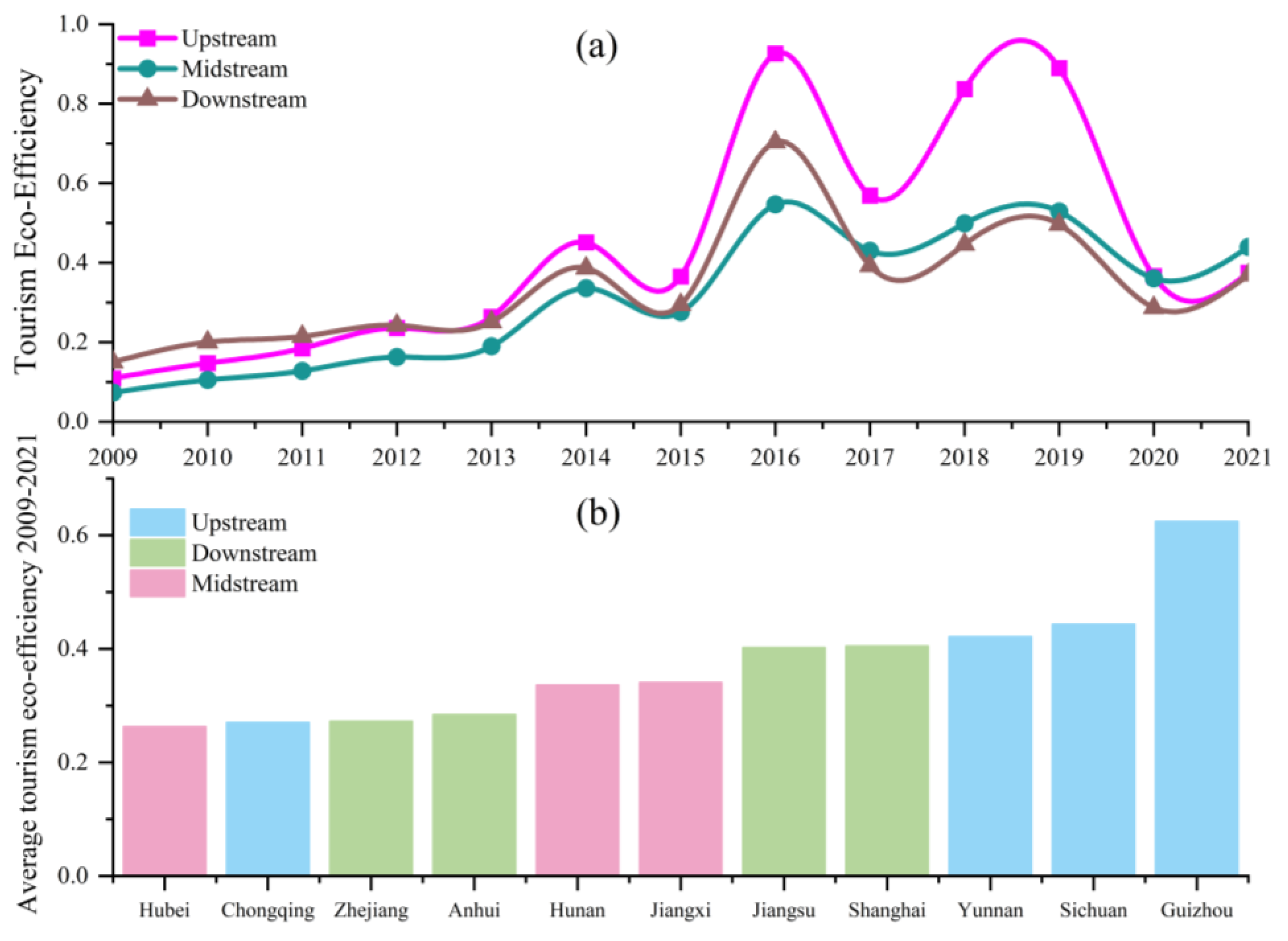
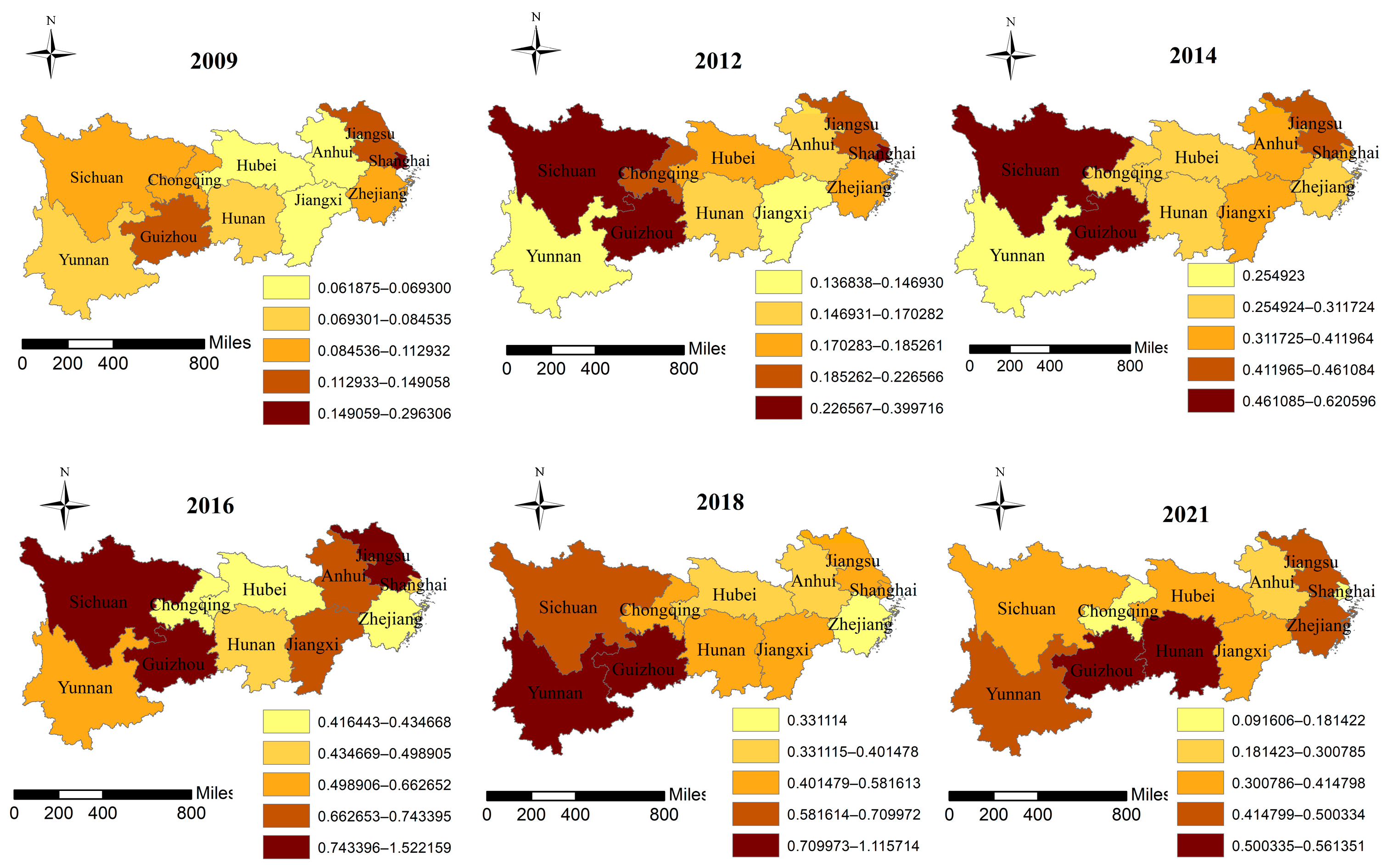
Region	2009	2010	2011	2012	2013	2014	2015	2016	2017	2018	2019	2020	2021
Shanghai	0.2963	0.3862	0.3729	0.3997	0.3696	0.3839	0.3699	0.4989	0.4900	0.5555	0.6247	0.3397	0.1814
Jiangsu	0.1367	0.1887	0.2081	0.2266	0.2527	0.4611	0.3206	1.1374	0.4252	0.4980	0.5530	0.3301	0.4947
Zhejiang	0.1069	0.1467	0.1596	0.1853	0.2099	0.2900	0.2685	0.4347	0.3160	0.3311	0.3445	0.2529	0.5003
Anhui	0.0619	0.0809	0.1185	0.1592	0.1723	0.4120	0.2196	0.7434	0.3387	0.4015	0.4645	0.2270	0.3008
Hubei	0.0659	0.1061	0.1339	0.1822	0.2395	0.2889	0.2806	0.4164	0.3450	0.3709	0.4027	0.2374	0.3546
Hunan	0.0845	0.1193	0.1409	0.1703	0.1625	0.3117	0.2507	0.4980	0.4664	0.5448	0.5643	0.5110	0.5502
Jiangxi	0.0693	0.0901	0.1097	0.1368	0.1674	0.4072	0.2952	0.7272	0.4795	0.5816	0.6211	0.3344	0.4148
Chongqing	0.1036	0.1397	0.1823	0.2161	0.2171	0.3107	0.2504	0.4208	0.3708	0.4835	0.6263	0.1058	0.0916
Guizhou	0.1491	0.1934	0.2578	0.2949	0.3667	0.6206	0.4992	1.5222	0.8058	1.1157	1.3120	0.4229	0.5614
Yunnan	0.0722	0.0965	0.1018	0.1469	0.1698	0.2549	0.2174	0.6627	0.5403	1.0384	1.0871	0.6279	0.4673
Sichuan	0.1129	0.1603	0.1978	0.2864	0.3018	0.6181	0.4960	1.1010	0.5598	0.7100	0.5349	0.3103	0.3796
Upstream	0.1094	0.1475	0.1849	0.2361	0.2638	0.4511	0.3658	0.9267	0.5692	0.8369	0.8901	0.3667	0.3750
Midstream	0.0733	0.1052	0.1282	0.1631	0.1898	0.3359	0.2755	0.5472	0.4303	0.4991	0.5293	0.3609	0.4399
Downstream	0.1504	0.2006	0.2148	0.2427	0.2511	0.3867	0.2947	0.7036	0.3925	0.4465	0.4967	0.2874	0.3693

.

The study reveals that the TEE generally exhibited a fluctuating upward trend over the research period, yet it failed to attain an optimal state. Specifically, the mean TEE value escalated from 0.1110 in 2009 to 0.3947 in 2021, peaking at 0.7258 in 2016. However, the mean value consistently remained below 1.000, signifying that the TEE has not yet achieved an optimal level.

From a regional economic perspective, there are regional disparities in the TEE. As depicted in Figure 3a, the upper reaches exhibit the highest efficiency values and the fastest growth during the sample period, increasing from 0.1094 in 2009 to 0.3750 in 2021. The efficiency levels of the middle and lower reaches are close, showing a fluctuating upward trend with alternating dominance; from 2009 to 2017, the lower reaches had higher efficiency than the middle reaches, while from 2017 to 2021, the middle reaches surpassed the lower reaches. Specifically, as shown in Figure 3b, the upper reaches, including Guizhou, Sichuan, and Yunnan, maintain relatively high efficiency values, whereas Chongqing has a lower efficiency, just above Hubei in the middle reaches. In the lower reaches, Jiangsu and Shanghai also show relatively high efficiency values, but Zhejiang and Anhui have lower efficiency values than Hunan and Jiangxi in the middle reaches. The spatial distribution analysis, exemplified by the years 2009, 2012, 2014, 2016, 2018, and 2021, and visualized in the spatial distribution map of TEE in the YREB (as shown in Figure 4), reveals a shift of high-efficiency regions from east to west with Guizhou as the core. In 2009, areas such as Shanghai, Jiangsu, and Guizhou had relatively high efficiency values, while the middle reaches generally had lower efficiency values. Between 2012 and 2018, the high-efficiency regions also included Sichuan and Yunnan. By 2021, the high-efficiency regions gradually shifted to areas in the middle reaches, such as Hunan. Overall, Guizhou and Jiangsu have consistently been on the best-practice frontier production surface, and the efficiency values in the upper and lower reaches are generally higher than those in the middle reaches.

4.1.2. Decomposition of Malmquist Model

To overcome the limitations of the discontinuous nature of the SBM-DEA model in assessing dynamic changes in TEE across periods in the YREB and to analyze the specific sources of these changes, this study employs the Malmquist index model for efficiency decomposition. The decomposition outcomes, segmented by year and region, are detailed in

Table 4. Annual Malmquist model decomposition results of TEE in the YREB, 2009–2021.

Year	Effch	Techch	Pech	Sech	Tfpch
2009–2010	1.0635	1.3245	1.1658	0.9478	1.4071
2010–2011	1.2822	0.9688	1.0271	1.3328	1.2169
2011–2012	1.1187	1.1276	1.0361	1.0807	1.2500
2012–2013	1.0686	1.0737	1.0835	0.9905	1.1392
2013–2014	0.9566	1.8855	0.9901	1.0154	1.7890
2014–2015	1.0654	0.7226	1.0828	0.9967	0.7708
2015–2016	0.9476	2.7948	0.9567	0.9932	2.5970
2016–2017	1.1246	0.6277	1.0984	0.9921	0.6648
2017–2018	0.9322	1.4019	0.9821	0.9617	1.2937
2018–2019	0.9653	1.1282	0.9597	1.0402	1.0871
2019–2020	1.1407	0.4837	1.2818	0.9772	0.5539
2020–2021	1.0050	1.2746	1.0284	0.9788	1.1997

and

Table 5. Regional Malmquist model decomposition results of TEE in the YREB, 2009–2021.

Region	Effch	Techch	Pech	Sech	Tfpch
Anhui	1.0929	1.2437	1.1096	0.9891	1.4426
Guizhou	1.0000	1.2228	1.0000	1.0000	1.2228
Hubei	1.0953	1.2153	1.0863	1.0128	1.2186
Hunan	1.1260	1.1730	1.0819	1.0349	1.2420
Jiangsu	1.0183	1.3383	1.0164	1.0260	1.3105
Jiangxi	1.0831	1.2056	0.9854	1.1432	1.3270
Shanghai	1.0229	1.2573	1.0238	0.9535	0.9932
Sichuan	1.0482	1.2086	1.0542	1.0346	1.2473
Yunnan	1.1145	1.2629	1.1282	1.1251	1.3940
Zhejiang	1.0593	1.2667	1.1489	1.0085	1.2017
Chongqing	0.9537	1.1848	1.0000	0.9537	1.1221
Upstream	1.0291	1.2198	1.0456	1.0284	1.2466
Midstream	1.1015	1.1980	1.0512	1.0636	1.2625
Downstream	1.0484	1.2765	1.0747	0.9943	1.2370
Whole territory	1.0559	1.2345	1.0577	1.0256	1.2474

.

During the period from 2009 to 2021, the overall TEE exhibited a fluctuating trend. As evident from Table 4 and Figure 5a, the tfpch across the YREB was generally above 1, suggesting an overall improvement in the relative efficiency of TEE. Both the technical efficiency and technological progress indices were predominantly greater than 1, indicating significant technological advancements and improvements in technical efficiency.

As depicted in Table 5 and Figure 5b, except for Shanghai, all other provinces and cities exhibited a TFP (Tfpch) greater than 1, indicating a relative enhancement in TEE during the study period. The technological progress index (Techch) of all 11 provinces and cities surpassed 1, reflecting substantial technological advancements. The technical efficiency index (Effch) was greater than 1 for all regions except Chongqing, indicating a notable improvement in technical efficiency.

From a regional perspective, Shanghai demonstrated a lower average TEE but a faster growth rate, whereas Anhui Province had a higher average but the slowest growth rate. Notably, the enhancement in TFP was primarily attributed to pure technical efficiency within technological progress. Figure 5 highlights that the increase in TFP was primarily driven by technological progress, rather than an increase in technical efficiency. Within technological progress, the contribution of pure technical efficiency was significantly higher than that of scale efficiency.

4.2. Spatial Interaction Spillover Effect Test

4.2.1. Spatial Correlation Test

Moran’s I index, presented in

Table 6. Moran’s I index for core variables.

Variable	Moran’s I	E (I)	Sd (I)	Z	p-Value
TEE	0.447	−0.007	0.045	10.007	0.000 ***
RGDP	0.276	−0.007	0.045	6.213	0.000 ***

Notes: *** is significant levels of 1%.

, was employed to scrutinize the spatial autocorrelation of the core variables. Notably, during the study period, both core variables’ Moran’s I indices surpassed the 1% significance threshold, yielding positive values. This positive spatial autocorrelation between TEE and RGDP in the YREB necessitates a deeper investigation into spatial spillover effects.

4.2.2. Parameter Estimation

This paper presents the estimation results of the spatial econometric model using the GS3SLS method, as shown in

Table 7. Basic regression results.

Items		TEE			RGDP
	Coefficient	Std. Err.	t-Value	Coefficient	Std. Err.	t-Value
TEE	—	—	—	4.493 ***	0.500	8.98
RGDP	0.212 ***	0.041	5.18	—	—	—
W × TEE	0.940 ***	0.319	2.95	−4.192 ***	1.589	−2.64
W × RGDP	−0.118 **	0.057	−2.07	0.490 *	0.265	1.86
vissca	0.008	0.247	0.03	—	—	—
toureco	0.027	0.222	0.12	—	—	—
tourindustr	−0.381 ***	0.056	−6.84	—	—	—
scitech	−0.025	0.207	−0.12	0.223	0.799	0.28
urb	—	—	—	0.158	1.291	0.12
industr	—	—	—	0.181 ***	0.019	9.34
cons1	0.449 **	0.187	2.41	—	—	—
cons2	—	0.187	—	−2.099 **	0.919	−2.28
Adj_R2		0.8746			0.6320

Notes: *, **, and *** are significant levels of 10%, 5% and 1%, respectively.

. Table 7 reveals that both TEE and RGDP have passed significance tests to varying degrees, indicating a significant interaction effect and spatial spillover effect between the two.

(1)

General interaction effect analysis

The estimates from the simultaneous equations model indicate that the RGDP has a significant positive regression coefficient of 0.212 within the TEE equation, suggesting a 21.2% increase in eco-efficiency for each unit of economic development. Conversely, in the RGDP equation, TEE exhibits a regression coefficient of 4.493, also significantly positive, implying a 4.493-unit escalation in economic development for each unit of eco-efficiency improvement. This highlights a strong interdependence between the two variables, with TEE exerting a greater influence on RGDP.

The enhancement in TEE signifies an increased focus on ecological conservation during tourism development, which in turn fosters the sustainable utilization of ecological resources. As ecological resources are crucial for tourism growth, their sustainable use is essential for economic progress. Furthermore, a higher level of economic development provides a larger capital base to support tourism, including infrastructure construction, resource conservation, and exploitation. Additionally, economic growth-driven technological advancements introduce advanced environmental protection technologies and methodologies to the tourism industry, thereby contributing to an improvement in TEE.

(2)

Spatial interactive spillover effect analysis

The regression coefficient on the spatial lag term in the TEE equation significantly indicates that the spatial lag of RGDP (W × RGDP) surpasses the 5% significance level, exhibiting a negative sign. This observation underscores the suppressive impact of economic growth in neighboring regions on the enhancement of local TEE. The intensifying economic development in adjacent areas frequently leads to heightened competition for tourism resources, encompassing the quest for tourists and tourism investments. Such rivalry may compel local tourism industries to prioritize short-term profit maximization strategies, often disregarding ecological and environmental conservation, thereby deteriorating TEE. Within the framework of the RGDP equation, the regression coefficient linked to the spatial lag of TEE (W × TEE) also exhibits a significant negative value, suggesting that the TEE of neighboring regions impedes local economic development. As TEE improves in adjacent regions, they tend to harness and develop tourism resources more effectively, attracting a larger influx of tourists and investments. This trend can lead to a relative decline in the attractiveness of local tourism resources, resulting in a reduction in tourist flow and investment inflow, thereby hampering local economic development. Furthermore, as the TEE progresses in neighboring regions, they offer enhanced tourism products and services that cater to the higher-level demands of tourists. This shift may motivate tourists to prefer neighboring regions as their preferred tourism destinations, bypassing local ones, and thereby diminishing local tourism revenue and employment opportunities.

5. Discussion

5.1. Measurement, Dynamics, and Causes of Change in TEE

Initially, this study utilized the super SBM-DEA model and the Malmquist index model to quantify the TEE of 11 provinces and cities within China’s YREB spanning the years 2009 to 2021. During the study period, the TEE exhibited a general upward trajectory interspersed with notable fluctuations, alongside pronounced inter-regional disparities. Notably, the upstream regions exhibited the highest efficiency levels and the fastest growth throughout the sample period, whereas the middle and downstream regions displayed relatively similar efficiency levels, fluctuating in an alternating ascending pattern. This aligns with China’s current developmental context, wherein the economically advanced eastern regions display less decoupling, whereas the less financially developed central and western regions demonstrate better decoupling levels [36]. Furthermore, it highlights the potential for improving TEE, which could be achieved through policy guidance and support, the enactment and enforcement of stringent environmental regulations, and the innovation and application of technologies aimed at reducing environmental costs and enhancing TEE.

From a dynamic perspective, the Tfpch value generally exceeded 1 during the research period, signifying an enhancement in relative efficiency. This advancement can be ascribed to the YREB’s strengthened implementation of environmental regulations, encompassing pollution emission standards and resource utilization efficiency mandates, aimed at maintaining tourism activities within ecological thresholds. Regarding the causes of dynamic changes, the Malmquist index decomposition revealed that the improvement in TEE specifically stems from technological progress rather than technical efficiency; moreover, within technological progress, the enhancement of pure technical efficiency significantly outweighs the improvement in scale efficiency. This may be due to factors such as resource constraints, environmental restrictions, or market saturation in the YREB, where scale expansion has not led to the expected efficiency improvements. In comparison, enhancing pure technical efficiencies, such as through improved management and operational processes, may provide a more sustainable and effective impetus for the growth of TEE. Additionally, the YREB may have experienced significant technological innovations that directly enhance TEE rather than merely relying on more effective use of existing technologies.

5.2. Spatial Interaction Spillovers between TEE and RGDP

From the perspective of general interaction effects, a mutually reinforcing relationship exists between TEE and RGDP. On one hand, RGDP directly increases residents’ disposable income, which in turn boosts the scale of tourism consumption. This is consistent with the force analysis results presented earlier [26], and to a certain extent, it promotes the improvement of the TEE. On the other hand, regional economic development contributes to improving infrastructure and public services, fosters the development of tourism industry clusters, and enhances sustainable development, thereby improving the TEE.

Conversely, the enhancement of TEE also benefits RGDP. Firstly, it creates employment opportunities. The sustained development of the tourism industry can drive the supply of related sectors, provide substantial job opportunities for residents, increase their income levels, and thus promote RGDP. Secondly, it promotes the coordinated development of the regional economy. The tourism industry has a long-related industry chain and includes a wide range of sectors, and its development helps facilitate the coordinated development of the regional economy.

Additionally, considering spatial interactive spillover effects, this study finds that the economic growth of neighboring regions has a siphoning impact on the improvement of the local TEE, and the enhancement of the neighboring TEE has a suppressive effect on regional economic development. This is consistent with the theoretical analysis section [31,35].

6. Conclusions and Suggestions

6.1. Conclusions

This study uses the super SBM-DEA model and Malmquist model to measure the tourism eco-efficiency (TEE) of the YREB, revealing dynamic changes and technological progress as the leading causes. We propose fundamental suggestions to enhance TEE, guide tourism planning, and quantify spatial spillover effects between TEE and RGDP. This paper contributes to the selection of methods for measuring tourism ecological efficiency by selecting those that can reveal the dynamic tourism ecological efficiency and reflect the reasons for changes. In addition, this article identifies and quantifies the complex bidirectional interaction between tourism ecological efficiency and regional economic development and reveals the spatial correlation between the two. The spatial relationship between TEE and RGDP is quite complex, and may even become more intricate due to differences in regional economic development levels and resource endowments. The spatial spillover effect will also be affected by the differences in economic development levels among provinces and whether there will be differences in different regions is also a part of future research. In addition, refining the research scale to the urban level is also one of the future research directions.

6.2. Suggestions

From the above discussion, this paper makes the following recommendations:

(1)

Promoting technological innovation and minimizing energy consumption are imperative. The research underscores technological progress as the pivotal force in enhancing TEE. Hence, augmenting investments in technological innovation is essential. Firstly, the tourism industry must intensify investments in advanced eco-friendly technologies to mitigate resource consumption and waste generation, thereby directly enhancing the ecological efficiency of tourism activities and mitigating their environmental impact. Secondly, harnessing new-generation information technologies, including the Internet of Things (IoT), big data, and artificial intelligence, to empower intelligent management systems is crucial. This enables real-time monitoring and data analysis, optimizing resource allocation and energy utilization, refining tourist flow management, minimizing resource waste, and offering personalized services, ultimately enhancing TEE.

(2)

To bolster the leading radiating role and foster positive spillover effects, administrative regional barriers must be dismantled to allow high-efficiency regions like Jiangsu and Guizhou to fully exert their influence. This will facilitate green and low-carbon cooperation among provinces and cities in the region, promoting the integrated and coordinated development of the low-carbon tourism industry. The aim is to establish a carbon reduction spatial pattern for tourism industry development that aligns with development positioning and regional collaborative complementarity, thereby contributing to the green demonstration construction and regional collaborative development of the YREB.

(3)

In adjusting the tourism industry structure and achieving cross-regional collaboration, it is noteworthy that while TEE and RGDP exhibit an interactive relationship with mutual reinforcement, TEE plays a more pivotal role and exerts a more substantial positive impact. By embarking on cross-regional cooperative projects, such as ecological tourism corridors and green tourism networks, we can strengthen the integration of tourism resources and market sharing between provinces, achieve the spatial spillover effect of TEE, and ultimately drive the coordinated development of the regional economy.

References

- Godil, D.I.; Sharif, A.; Rafique, S.; Jermsittiparsert, K. The asymmetric effect of Tourism, Financial development and Globalization on Ecological footprint in Turkey. Environ. Sci. Pollut. Res. 2020, 27, 40109–40120. [Google Scholar] [CrossRef] [PubMed]
- Gössling, S. Carbon neutral destinations: A conceptual analysis. J. Sustain. Tour. 2009, 17, 17–37. [Google Scholar] [CrossRef]
- Han, H. Consumer behavior and environmental sustainability in tourism and hospitality: A review of theories, concepts, and latest research. Sustain. Consum. Behav. Environ. 2021, 29, 1–22. [Google Scholar]
- Lenzen, M.; Sun, Y.Y.; Faturay, F.; Ting, Y.P.; Geschke, A.; Malik, A. Author Correction: The carbon footprint of global tourism. Nat. Clim. Chang. 2018, 8, 544. [Google Scholar] [CrossRef]
- Wang, S.L.; Li, Y.C.; Zhang, C.P. Analysis of the Effect of Social Support on Sustainable Competitive Advantage in Tourism Industry—Based on the Perspective of Living-Ecology-Production Integrated Space. Rev. Cercet. Interv. Soc. 2020, 71, 250–263. [Google Scholar] [CrossRef]
- Zhang, Y.; Khan, S.U.; Swallow, B.; Liu, W.; Zhao, M. Coupling coordination analysis of China’s water resources utilization efficiency and economic development level. J. Clean. Prod. 2022, 373, 133874. [Google Scholar] [CrossRef]
- Kong, Y.; Liu, S. Spatio-temporal Evolution and Driving Factors of Carbon Dioxide Emissions from Energy Consumption in the Yellow River Basin. J. Phys. Conf. Ser. 2023, 2468, 012124. [Google Scholar] [CrossRef]
- Perch-Nielsen, S.; Sesartic, A.; Stucki, M. The greenhouse gas intensity of the tourism sector: The case of Switzerland. Environ. Sci. Policy 2010, 13, 131–140. [Google Scholar] [CrossRef]
- Sun, J.; Tang, D.; Kong, H.; Boamah, V. Impact of Industrial Structure Upgrading on Green Total Factor Productivity in the Yangtze River Economic Belt. Int. J. Environ. Res. Public Health 2022, 19, 3718. [Google Scholar] [CrossRef]
- Wu, C.; Zhuo, L.; Chen, Z.; Tao, H. Spatial Spillover Effect and Influencing Factors of Information Flow in Urban Agglomerations—Case Study of China Based on Baidu Search Index. Sustainability 2021, 13, 8032. [Google Scholar] [CrossRef]
- Liu, J.; Zhang, J.; Fu, Z. Tourism eco-efficiency of Chinese coastal cities—Analysis based on the DEA-Tobit model. Ocean Coast. Manag. 2017, 148, 164–170. [Google Scholar] [CrossRef]
- Gössling, S.; Peeters, P.; Ceron, J.P.; Dubois, G.; Patterson, T.; Richardson, R.B. The eco-efficiency of tourism. Ecol. Econ. 2005, 54, 417–434. [Google Scholar] [CrossRef]
- Ruan, W.Q.; Li, Y.Q.; Zhang, S.N.; Liu, C.H. Evaluation and drive mechanism of tourism ecological security based on the DPSIR-DEA model. Tour. Manag. 2019, 75, 609–625. [Google Scholar] [CrossRef]
- Becken, S. Developing indicators for managing tourism in the face of peak oil. Tour. Manag. 2008, 29, 695–705. [Google Scholar] [CrossRef]
- Liu, Q.; Song, J.; Dai, T.; Xu, J.; Li, J.; Wang, E. Spatial Network Structure of China’s Provincial-Scale Tourism Eco-Efficiency: A Social Network Analysis. Energies 2022, 15, 1324. [Google Scholar] [CrossRef]
- Liu, Y.; Zhu, J.; Li, E.; Meng, Z.; Song, Y. Environmental regulation, green technological innovation, and eco-efficiency: The case of Yangtze River Economic Belt in China. Technol. Forecast. Soc. Chang. 2020, 155, 119993. [Google Scholar] [CrossRef]
- Zhang, M.L.; Cheng, Z. Research on carbon emission efficiency in the Chinese construction industry based on a three-stage DEA-Tobit model. Environ. Sci. Pollut. Res. 2021, 28, 51120–51136. [Google Scholar] [CrossRef]
- Kytzia, S.; Walz, A.; Wegmann, M. How can tourism use land more efficiently? A model-based approach to land-use efficiency for tourist destinations. Tour. Manag. 2011, 32, 629–640. [Google Scholar] [CrossRef]
- Tsionas, E.; Assaf, A. Short-run and long-run performance of international tourism: Evidence from Bayesian dynamic models. Tour. Manag. 2014, 42, 22–36. [Google Scholar] [CrossRef]
- Carboni, O.A.; Russu, P. Measuring and forecasting regional environmental and economic efficiency in Italy. Appl. Econ. 2018, 50, 335–353. [Google Scholar] [CrossRef]
- Zha, J.; Yuan, W.; Dai, J.; Tan, T.; He, L. Eco-efficiency, eco-productivity and tourism growth in China: A non-convex metafrontier DEA-based decomposition model. J. Sustain. Tour. 2020, 28, 663–685. [Google Scholar] [CrossRef]
- Fan, Y.; Bai, B.; Qiao, Q.; Kang, P.; Zhang, Y.; Guo, J. Study on eco-efficiency of industrial parks in China based on data envelopment analysis. J. Environ. Manag. 2017, 192, 107–115. [Google Scholar] [CrossRef] [PubMed]
- Jiang, Z.; Guo, F.; Cai, L.; Li, X. Eco-Province Construction Performance and Its Influencing Factors of Shandong Province in China: From Regional Eco-Efficiency Perspective. Sustainability 2021, 13, 12068. [Google Scholar] [CrossRef]
- Tsaur, S.H.; Lin, Y.C.; Lin, J.H. Evaluating ecotourism sustainability from the integrated perspective of resource, community and tourism. Tour. Manag. 2006, 27, 640–653. [Google Scholar] [CrossRef]
- Erol, I.; Neuhofer, I.O.; Dogru, T.T.; Oztel, A.; Searcy, C.; Yorulmaz, A.C.J.T.M. Improving sustainability in the tourism industry through blockchain technology: Challenges and opportunities. Tour. Manag. 2022, 93, 104628. [Google Scholar] [CrossRef]
- Zhang, L.; Gao, J. Exploring the effects of international tourism on China’s economic growth, energy consumption and environmental pollution: Evidence from a regional panel analysis. Renew. Sustain. Energy Rev. 2016, 53, 225–234. [Google Scholar] [CrossRef]
- Nugroho, P.; Numata, S. Resident support of community-based tourism development: Evidence from Gunung Ciremai National Park, Indonesia. J. Sustain. Tour. 2020, 30, 2510–2525. [Google Scholar] [CrossRef]
- Xu, T.; Lv, Z. Does too much tourism development really increase the size of the informal economy? Curr. Issues Tour. 2022, 25, 844–849. [Google Scholar]
- Bazargani, R.H.; Kili, H. Tourism competitiveness and tourism sector performance: Empirical insights from new data. J. Hosp. Tour. Manag. 2021, 46, 73–82. [Google Scholar] [CrossRef]
- Wang, X.Y.; Chai, Y.Z.; Wu, W.S.; Khurshid, A. The Empirical Analysis of Environmental Regulation’s Spatial Spillover Effects on Green Technology Innovation in China. Int. J. Environ. Res. Public Health 2023, 20, 1069. [Google Scholar] [CrossRef]
- Luo, K.; Liu, Y.; Chen, P.F.; Zeng, M. Assessing the impact of the digital economy on green development efficiency in the Yangtze River Economic Belt. Energy Econ. 2022, 112, 106127. [Google Scholar] [CrossRef]
- Chen, C.; Bi, L.; Zhu, K. Study on Spatial-Temporal Change of Urban Green Space in Yangtze River Economic Belt and Its Driving Mechanism. Int. J. Environ. Res. Public Health 2021, 18, 12498. [Google Scholar] [CrossRef] [PubMed]
- Liu, J.; Feng, T.; Yang, X. The energy requirements and carbon dioxide emissions of tourism industry of Western China: A case of Chengdu city. Renew. Sustain. Energy Rev. 2011, 15, 2887–2894. [Google Scholar] [CrossRef]
- Zhang, R.; Ma, Y.; Ren, J. Green Development Performance Evaluation Based on Dual Perspectives of Level and Efficiency: A Case Study of the Yangtze River Economic Belt, China. Int. J. Environ. Res. Public Health 2022, 19, 9306. [Google Scholar] [CrossRef]
- Cheng, Y.F.; Zhu, K.; Zhou, Q.; El Archi, Y.; Kabil, M.; Remenyik, B.; Dávid, L.D. Tourism Ecological Efficiency and Sustainable Development in the Hanjiang River Basin: A Super-Efficiency Slacks-Based Measure Model Study. Sustainability 2023, 15, 6159. [Google Scholar] [CrossRef]
- Tang, Q.L.; Wang, Q.Q.; Zhou, T.C. Driving Forces of Tourism Carbon Decoupling: A Case Study of the Yangtze River Economic Belt, China. Sustainability 2022, 14, 8674. [Google Scholar] [CrossRef]
- Li, S.; Ren, T.; Jia, B.; Zhong, Y. The Spatial Pattern and Spillover Effect of the Eco-Efficiency of Regional Tourism from the Perspective of Green Development: An Empirical Study in China. Forests 2022, 13, 1324. [Google Scholar] [CrossRef]
- Zhang, W.; Zhan, Y.; Yin, R.Y.; Yuan, X.B. The Tourism Eco-Efficiency Measurement and Its Influencing Factors in the Yellow River Basin. Sustainability 2022, 14, 15654. [Google Scholar] [CrossRef]
- Zhang, F.T.; Yang, X.Y.; Wu, J.F.; Ma, D.L.; Xiao, Y.D.; Gong, G.F.; Zhang, J.Y. How New Urbanization Affects Tourism Eco-Efficiency in China: An Analysis Considering the Undesired Outputs. Sustainability 2022, 14, 10820. [Google Scholar] [CrossRef]
- Cheng, L.; Zhou F, Y. Research on the Spatiotemporal Pattern and Growth Effect of Tourism Ecological Efficiency in the Yangtze River Economic Belt. J. Chongqing Technol. Bus. Univ. 2024, 37, 835–848. (In Chinese) [Google Scholar]
- Jin, J.; Kim, D. Expansion of the subway network and spatial distribution of population and employment in the Seoul metropolitan area. Urban Stud. 2018, 55, 2499–2521. [Google Scholar] [CrossRef]
- Li, Y.F.; Li, J.; Xu, M. The interaction multiplier and spatial spillover effect between manufacturing employment and service employment. Financ. Trade Econ. 2017, 38, 115–129. (In Chinese) [Google Scholar]