Article

Land Cover and Spatial Distribution of Surface Water Loss Hotspots in Italy

Department of Civil, Chemical, Environmental, and Materials Engineering, Alma Mater Studiorum Università di Bologna, 40136 Bologna, Italy
*
Author to whom correspondence should be addressed.
Sustainability 2024, 16(18), 8021; https://doi.org/10.3390/su16188021
Submission received: 4 July 2024 / Revised: 9 September 2024 / Accepted: 10 September 2024 / Published: 13 September 2024

Abstract

:
Increasing water withdrawals and changes in land cover/use are critically altering surface water bodies, often causing a noticeable reduction in their area. Such anthropogenic modification of surface waters needs to be thoroughly examined to recognize the dynamics through which humans affect the loss of surface water. By leveraging remotely-sensed data and employing a distance–decay model, we investigate the loss of surface water resources that occurred in Italy between 1984 and 2021 and explore its association with land cover change and potential human pressure. In particular, we first estimate the land cover conversion across locations experiencing surface water loss. Next, we identify and analytically model the influence of irrigated and built-up areas, which heavily rely on surface waters, on the spatial distribution of surface water losses across river basin districts and river basins in Italy. Our results reveal that surface water losses are mainly located in northern Italy, where they have been primarily replaced by cropland and vegetation. As expected, we find that surface water losses tend to be more concentrated in the proximity of both irrigated and built-up areas yet showing differences in their spatial occurrence and extent. These observed spatial patterns are well captured by our analytical model, which outlines the predominant role of irrigated areas, mainly across northern Italy and Sicily, and more dominant effects of built-up areas across the Apennines and in Sardinia. By highlighting land cover patterns following the loss of surface water and evaluating the relative distribution of surface water losses with respect to areas of human pressure, our analysis provides key information that could support water management and prevent future conditions of water scarcity due to unsustainable water exploitation.

1. Introduction

Surface water represents a key water source for many human purposes, including, e.g., irrigation in agricultural areas and industrial and domestic water supply in urban areas [1,2,3]. Surface water bodies have been continuously altered by humans, who have deteriorated aquatic ecosystems and have harmed local and global economies, increasing the risk of water shortages [4,5,6]. During the period 1971–2000, anthropogenic water consumption produced a mean annual decrease in the runoff of at least 5% in many river basins, with more prominent impacts in heavily irrigated areas [7]. Similarly, over the last three decades, unsustainable water consumption and a changing climate have caused considerable storage losses in more than half of the largest global lakes [8]. A recent study has shown that 61% of the global variability in seasonal surface water storage occurs in river basins with human-managed reservoirs [9].
Irrigation is the most water-intensive sector, accounting for about 70% of global freshwater withdrawals worldwide, with approximately two-thirds of the global irrigated area dependent on surface water from rivers and lakes [10,11,12,13]. As surface water resources are also used to meet almost 80% of water demand in large urban cities, urban population growth, and the subsequent expansion of built-up areas are additional drivers of changes in surface water availability [14,15,16,17]. Future socio-economic development and climate change are expected to intensify water demand across all sectors [7,12,18,19,20], and the resulting human-driven losses of surface water suggest that the conservation of surface water bodies should be a priority in both water policy and urban planning [17,21].
Addressing water shortages has become a major challenge in the southern Mediterranean region, where climate change and increasing human pressure are severely impacting water availability [22,23,24,25]. In particular, in Italy, the issue of water scarcity is attracting increasing attention because of the frequent water shortages occurring across the whole country [25,26]. Even though the overall water availability across Italy is abundant, the unevenly spatiotemporal distribution of precipitation determines a heterogeneous distribution of water resources across the country, which could be insufficient to meet water demands [27]. More than half (53%) of the available surface water is located in northern Italy, about 40% is equally split between central and southern Italy, and the remaining 7% is found in the insular regions [28,29]. Surface water from rivers and lakes is the main source of freshwater withdrawals, providing about two-thirds of the total water abstraction in Italy [27,30]. Rivers represent the primary source in the agricultural sector, which actively influences river outflow patterns and the management of lakes and reservoirs [30]. Irrigation uses the majority (60%) of total water withdrawals [28] and sustains more than half of the Italian agricultural production [31], with water withdrawals mainly occurring in northern (67%) and southern Italy (13%) [32]. The industrial and energetic sectors account for 25% of total water withdrawals [28], and more than half of water abstractions for manufacturing industries occur in northern Italy [32]. However, the overall industrial use of surface water is relatively small [30]. As for public water supply, the domestic sector uses 15% of total water withdrawals [28]. Even though groundwater and springs generally provide water for civil uses, southern Italy and the insular regions derive up to 30% of household supply and drinking water from surface water [27,30,33]. During the last few decades, the runoff of Italian rivers has generally declined [34], and such a decrease was due not only to a reduction in annual precipitation (rain and snow) but also to an expansion of cultivated and urban areas [25,35,36,37]. However, human pressure on surface water depletion still remains underexplored in Italy. Moreover, even though satellite remote sensing provides high-resolution data for the monitoring and detection of inland surface water dynamics and land use/land cover change at the global scale [38,39,40,41,42,43,44,45,46,47,48], the application of such data to investigate the influence of anthropogenic activities on surface water over the Italian peninsula is still lacking.
Here, we investigate the loss in surface water resources that occurred in Italy between 1984 and 2021 and explore its association with land cover change and potential human pressure. Surface water loss is here defined as a transition from a water state in 1984 to a not-water state in 2021, leading to a decrease in the spatial extent of surface water bodies. We combine remotely sensed datasets to (1) estimate the land cover change across surface water loss (SWL) locations, (2) identify the SWL spatial distribution with respect to irrigated and built-up areas that heavily rely on surface waters, and (3) analytically reproduce this influence using a distance–decay model [16]. By disclosing how the loss of surface water is linked to land cover change and anthropogenic activities, this study improves our current understanding and may support the definition of sustainable and integrated water management policies for the prevention of water scarcity [1,10].

2. Materials and Methods

2.1. Study Area

We focused our analysis on Italy, a region particularly vulnerable to water scarcity due to a combination of climate change effects and an extensive human pressure on water resources [37,49,50]. Italy holds the largest irrigable area among the southern European countries [51,52] that requires considerable water withdrawals, especially during prolonged drought periods [21,31,53]. Italy also presents a heterogeneous distribution of human settlements, characterized by different sizes and distinct levels of urbanization [54,55,56], which can trigger a decrease in the spatial extent of surface water bodies.
To explore differences within the country, we consider two distinct spatial aggregations: river basins (RBs) and river basin districts (RBDs). As shown in Figure 1a, Italy comprises 137 RBs and 7 RBDs (i.e., Po, Eastern Alps, Northern Apennines, Central Apennines, Southern Apennines, Sicily, Sardinia; see also Table 1). An RBD encompasses several neighboring RBs and the associated groundwater and coastal waters. RBDs represent the main unit for the management of RBs and are governed by a specific administrative authority (the River Basin District Authority) [32]. RBDs have a similar extent and entirely cover the Italian territory, unlike RBs, which cover only 83.96% of Italy and thus provide a partial description of surface water loss, especially in the southeastern part of Italy (see Figure 1a).

2.2. Estimation of Land Cover Conversion across Surface Water Loss Hotspots

To identify the location of surface water loss (SWL) hotspots, we employed the Global Surface Water dataset [38], which provides multiple layers describing the location and temporal distribution of surface waters at the global scale approximately over the last four decades. This dataset was selected for its high temporal and spatial resolution and extensive validation [57]. Among all the available products, we adopted the Transitions layer, which shows changes in water seasonality between 1984 and 2021 at a 30 m spatial resolution and describes the conversion between permanent water, seasonal water, and no water (i.e., land) by categorizing these changes in specific classes. Among all the available classes, we selected lost permanent and lost seasonal surface water pixels to determine the location and extent of surface water losses in Italy. We also computed the relative loss of surface water (%) as compared to the total extent observed in 1984. Table 1 and Table A1 provide the spatial extent of SWL at the RBD and RB level, respectively. In particular, for RBs, we analyzed and reported data only for RBs with an SWL area > 0.5 km2.
Figure 1. Study area and remotely sensed data. (a) River Basins (RBs) and River Basin Districts (RBDs) across Italy; (b) land cover data from [58] within the Po RBD, as an example of the dataset; (c) the spatial distribution of irrigated and built-up areas from [59] within the Po RBD, as an example of the datasets.
Sustainability 16 08021 g001
In order to interpret the human-induced mechanism of surface water loss and its possible driving processes, it is crucial to assess the land cover change in SWL hotspots, which could offer insightful recommendations for water conservation strategies. We employed the ESA WorldCover product (version 2) for the year 2021 [58] to determine land cover classes corresponding to the location of SWL hotspots. This dataset includes 11 classes and has a 10 m spatial resolution, providing land cover information with an unprecedented resolution. Beyond its high level of accuracy, the ESA WorldCover product is particularly suitable for our analysis as it presents land cover observed in 2021, i.e., at the end of the period examined by the Transition layer of the Global Surface Water dataset [38]. To guarantee consistency in spatial resolutions among the datasets used in our analysis, we resample the WorldCover map to 30 m resolution. This involves coarsening the resolution of land cover data to match that of the surface water data, enabling an accurate assignment of land cover classes to SWL locations. As an example, Figure 1b shows a zoom in of the 2021 land cover map derived from the ESA WorldCover product within the Po RBD. Table 1 shows the main land cover in each RBD, whereas a detailed description of the distribution of all land cover classes across the examined RBDs and RBs is provided in Table A2 and Table A3, respectively.

2.3. Identification of the Spatial Distribution of Surface Water Loss Hotspots with Respect to Irrigated and Built-Up Areas

We employed the Corine Land Cover (CLC) 2018 dataset [59] to identify the distribution of irrigated and built-up areas. This dataset provides the most recent and detailed land cover and land use classification in Europe (44 land cover classes), which allowed us to accurately delineate irrigated and built-up areas that may have influenced the occurrence of SWL during the period of 1984–2021. The selected classes for irrigated areas were as follows: permanent irrigated land, rice fields, vineyards, fruit trees and berry plantations, olive groves, complex cultivation patterns, and land principally occupied by agriculture, with significant areas of natural vegetation. For built-up areas, we selected the following classes: continuous urban fabric, discontinuous urban fabric, industrial and commercial units, road and rail networks and associated land, port areas, airports, mineral extraction, dumps, construction sites, green urban areas, and sport and leisure facilities. To homogenize the resolution of all datasets, we resampled the CLC data from its original 100 m spatial resolution to the 30 m resolution of surface water data. The overall extent of irrigated and built-up areas at the RBD and RB level is reported in Table 1 and Table A1, respectively.
Then, we evaluated the spatial behavior of SWL hotspots by analyzing their occurrence as a function of the distance from three alternative areas of human pressure, namely the following:
  • Irrigated areas (IRR);
  • Built-up areas (BUP);
  • Anthropogenic areas (ANT), indicating areas of either irrigation practices, or human settlements (i.e., the sum of IRR and BUP areas).
We first identified clusters (i.e., pixel aggregations) of IRR, BUP, and ANT areas and computed the Euclidean distance of SWL hotspots from such areas. We defined 1 km-wide distance bins, and for each bin, di, we calculated the frequency of occurrence of SWL hotspots with respect to IRR, BUP, and ANT areas across each RB and RBD. Afterwards, we evaluated the mean and the maximum distance of SWL from IRR, BUP, and ANT areas.

2.4. Analytical Representation of the Spatial Distribution of Surface Water Loss Hotspots with Respect to Irrigated and Built-Up Areas

We analytically reproduced the observed pattern of frequency of SWL occurrence with a distance–decay model (SWL-DD in what follows), originally designed in Palazzoli et al. (2022) [16]. Here, we applied the SWL-DD model to a completely different geographical context, and we expanded its scope to illustrate the spatial influence of both irrigated and built-up areas, unlike the previous study, which focused solely on urban influence across the US.
The SWL-DD model describes the exponential decline in the probability of SWL occurrence, px(di), as a function of the distance, di, from an area of human pressure, x, as follows:
p x d i = α x e β x d i
where di is the 1 km-wide distance bin (going from 0 km to the maximum distance reached by SWL hotspots from the considered area of human pressure x) and αx and βx are the model parameters. In particular, αx [-] represents the frequency of occurrence of SWL hotspots within the first km, whereas βx (>0 [km−1]) estimates the decay rate of SWL occurrence. The model parameters are estimated with a non-linear regression of the frequency of SWL occurrence, and we employed the Pearson’s correlation coefficient, r, to evaluate the goodness of the fit. For further details about the modeling approach and a discussion of its assumptions, we refer the readers to Palazzoli et al. (2022) [16].
We adopted the 1 km-wide distance bins to group SWL hotspots, as this width offers the best compromise between noise reduction and level of resolution for the model fit application (i.e., at least three distance bins with a frequency of SWL occurrence ≠ 0 must be available). Moreover, in order to consider regions with a reasonable extent of SWL, we focused our analysis only on RBs having an SWL area greater than or equal to 0.5 km2, which reduced the number of RBs from 137 to 34. Despite this selection, in some RBs, the application of the model was still limited by the fact that SWL hotspots were all concentrated in the first distance bin.

3. Results

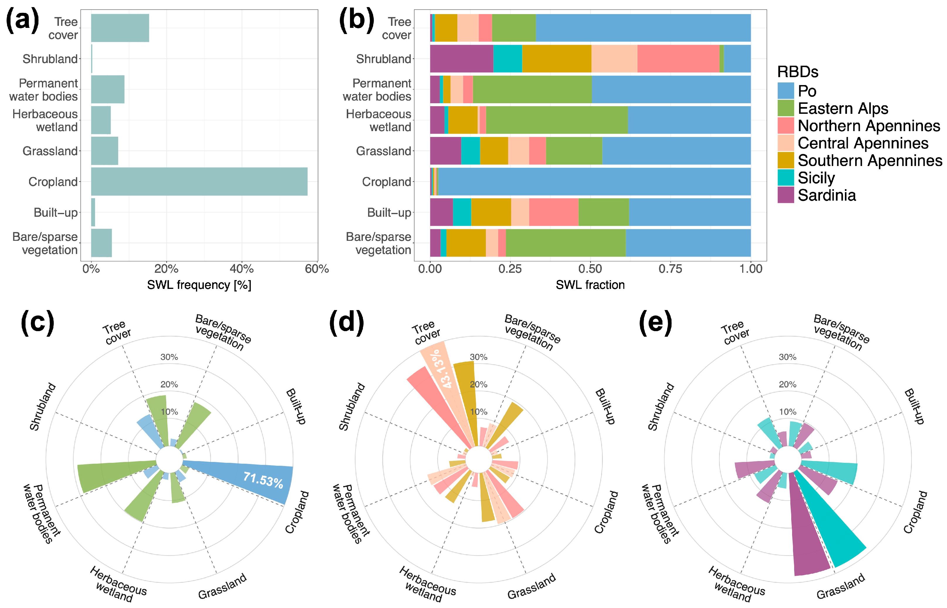
3.1. Observed Land Cover Conversion across Surface Water Loss Hotspots in Italy

From 1984 to 2021, about 7% of the total surface water extent in Italy has disappeared (667.74 km2), showing an uneven distribution of SWL across the country. We find that the majority of SWL hotspots (78.13%) are located within the Po RBD, followed by the Eastern Alps RBD (11.30%), while the rest of the RBDs include approximately 1% to 3.5% of the remaining SWL (Figure 2a and Table 1). The Po RBD also exhibits the largest reduction of the original extent of surface water (16.03%), followed by the Northern Apennines (9.33%) and Sicily (8.85%) RBDs (Table 1). A more detailed representation considering the 34 RBs with an SWL area ≥ 0.5 km2 is available in Table A1 and Figure 2b.
By coupling SWL hotspots and ESA WorldCover classes for 2021, we find that at the national level, almost 60% of SWL hotspots (corresponding to about 383.04 km2 of SWL area) faced a conversion into cropland, followed by tree cover (15%), permanent water bodies (8.71%), grassland (7.03%), bare/sparse vegetation (5.40%), herbaceous wetland (5.06%), built-up (0.94%), and shrubland (0.21%) classes (Figure 3a). As expected, some SWL hotspots are still classified as permanent water bodies in the 2021 land cover map. This discrepancy arises because SWL and land cover data derive from two independent datasets, i.e., the Global Surface Water dataset [38] and the ESA WorldCover product [58], which were developed using distinct methods of classification (Landsat versus Sentinel-1 and Sentinel-2 for [38] and [58], respectively). However, this disagreement does not compromise the robustness of our study, as it affects a relatively small fraction (<9%) of the total extent of SWL.
For each land cover class conversion, we analyze its spatial distribution across the RBDs (Figure 3b–e). Locations experiencing SWL across the Po RBD are now classified as cropland (71.53%), followed by tree cover (13.11%) (Figure 3c). In the Eastern Alps RBD, surface water is mainly replaced by herbaceous wetlands (19.84%), bare/sparse vegetation (19.84%), and tree cover (18.51%) (Figure 3c). In the Northern, Central, and Southern Apennines’ RBDs (Figure 3d), SWL hotspots are mostly associated with tree cover (34.31%, 43.13%, and 30.99%, respectively) and grassland (19.69%, 19.61%, and 17.79%, respectively) land cover classes. Similar trends in surface water conversion also characterize the Sicily and Sardinia RBDs (Figure 3e), with most of the SWL hotspots replaced by grassland (38.07% and 37.53%, respectively) and cropland (20.42% and 14.77%, respectively).

3.2. Observed Surface Water Loss Distribution across Italy

When analyzing the spatial distribution of SWL, we find that SWL hotspots are mainly concentrated around areas of human pressure and their frequency of occurrence declines as the distance from these areas increases (see dots in Figure 4 and Figure A1).
We find that SWL hotspots generally reach larger maximum distances from IRR areas (between 7 and 33 km) than from BUP areas (between 11 and 30 km) in all RBDs (Figure 5 and Table A4). As expected, maximum distances from ANT areas are characterized by smaller values (between 5 and 16 km) since IRR and BUP areas are combined together. The mean distance of SWL hotspots tend to be below 2 km from ANT and IRR areas and between 2 and 4 km from BUP areas. The results at the RB level are provided in Table A5.

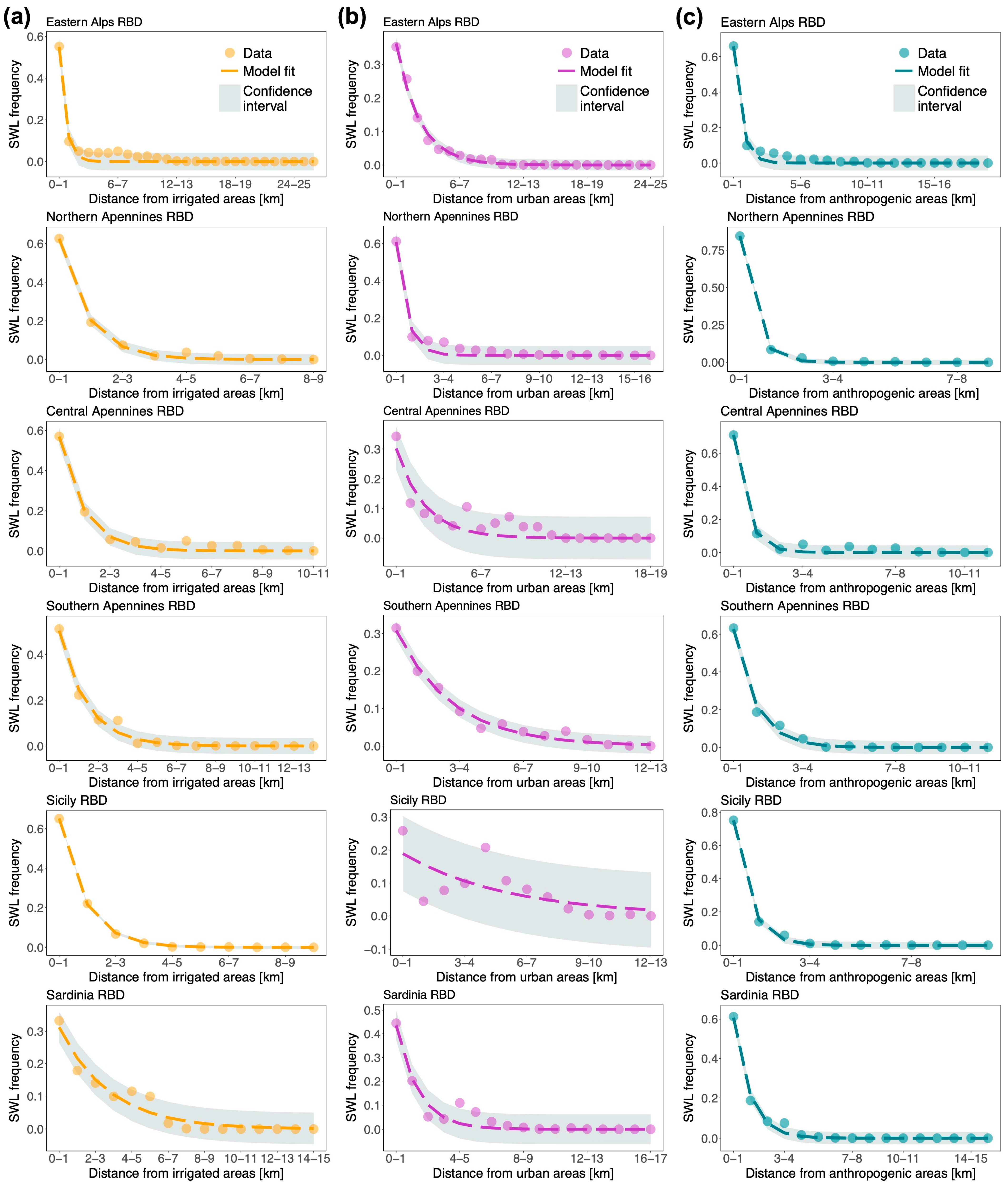
3.3. Modeled Surface Water Loss Distribution across Italy

We apply the SWL-DD model to all RBDs (see lines in Figure 4 and Figure A1) and to the 34 selected RBs. Our model successfully reproduces the spatial distribution of SWL hotspots with respect to any area of human pressure and across both spatial aggregations (Table A6 and Table A7), confirming the robustness of the proposed approach for built-up areas and, most importantly, extending for the first time its applicability to irrigated areas. When applying the model to RBs, we find that in two and six RBs (with respect to irrigated and anthropogenic areas, respectively), all SWL hotspots fall in the first distance bin, which impedes the model fit.
The correlation between the modeled and observed frequency of SWL occurrence with respect to IRR areas is above 0.99 at the RBD level (Table A6), while at the RB level, r values vary between 0.20 and 1.00, except for two RBs, in which the model cannot be applied due to data paucity (see Table A7).
Regarding BUP areas, the frequency of the occurrence of SWL hotspots from these regions is accurately modeled by the SWL-DD model, as proven by the correlation between observations and predictions, which is overall greater than 0.90 in all RBDs (Table A6) while ranging between 0.20 and 1.00 at the RB level (Table A7). A few exceptions are found for the Birgi and Biferno RBs, which show a mild increasing trend of the frequency of SWL occurrence (as confirmed by the negative values of the decay rate β), and for the Fortore RB, where SWL occurs up to 3 km from BUP areas. For these reasons, we prefer to exclude these RBs (highlighted by an asterisk in Table A7) from the forthcoming analysis.
The modeled distance decay of SWL occurrence from anthropogenic areas provides an excellent fit to the observed data, as proven by r values, which are around 1.00 in all RBDs (Table A6) and greater than 0.80 at the RB level (with the exception of the Carapelle, Coghinas, Lemene, and Vomano RBs, where r is less than 0.50, Table A7).
We estimate the values of the SWL-DD model parameters, α and β, and examine their distribution across the RBDs and RBs. The concentration of SWL hotspots in the first distance bin (0–1 km), as represented by α, is larger in the proximity of anthropogenic areas, followed by irrigated and built-up areas, with a median value at the RBD level equal to 0.71, 0.57, and 0.31, respectively (Figure 6). This result suggests that the spatial distribution of SWL hotspots with respect to anthropogenic areas usually mirrors the behavior observed for irrigated areas (Figure 6b–d). The only exception is the Sardinia RBD, which exhibits a larger concentration of SWL hotspots close to built-up areas (44%) rather than irrigated areas (31%) (Table A6). Overall, α shows the largest variability when it is computed with respect to irrigated and anthropogenic areas both across the RBDs and RBs (Figure 6a). A similar distribution of α values is also found at the RB level (Figure 6e–g), where the finer level of detail captures local patterns, which may differ from the regional ones. For instance, some RBs belonging to RBDs with relatively low α values show a higher frequency of SWL occurrence in the first distance bin (see, e.g., irrigated areas in the Crati RB within the Southern Apennines RBD and built-up areas in the Adige RB within the Eastern Alps RBD). Likewise, some other RBs show lower concentrations of SWL hotspots in the proximity of areas of human pressure than their respective RBDs (see, e.g., irrigated areas in the Simeto RB within the Sicily RBD and built-up areas in the Coghinas RB within the Sardinia RBD).
Moving to the spatial distribution of the decay rate of SWL occurrence, which is represented by β, we observe a faster decline (i.e., surface water losses are located within a shorter distance range from areas of human pressure) for anthropogenic areas, followed by irrigated and built-up ones (Figure 7). The values of β associated with built-up areas are larger than those for irrigated areas in the Northern Apennines and Sardinia RBDs, while the opposite pattern is found across the remaining RBDs (Figure 7b–d and Table A6). This indicates that in most of the RBDs, a higher concentration of SWL hotspots in the proximity of irrigated (or built-up) areas (i.e., higher α) usually corresponds to a faster decay in SWL occurrence from irrigated (or built-up) areas (i.e., higher β). We find only a couple of exceptions to this general trend at the RB level, where the Brenta and Sile RBs show a larger concentration of SWL hotspots close to built-up areas and a faster decline of SWL occurrence from irrigated areas (Table A7). Similarly to what we found for α, some RBs reveal specific patterns of β that do not align with the general trend of their RBD, proving once again that at a smaller scale, the influence of any area of human pressure may exert a stronger or weaker influence on the spatial decline of SWL occurrence (Figure 7e–g).

4. Discussion

We investigate the loss of surface water resources (defined as a conversion of permanent/seasonal surface water into land) that occurred in Italy between 1984 and 2021 across RBD and RB spatial aggregations, using remotely sensed data with high spatial resolution. In particular, we focus our attention on the influence of relevant human activities on losses of surface water, neglecting potential effects due to changes in climatic forcings. To do so, we quantify the overall extent of SWL and examine the subsequent associated land cover classes. We then analyze and model the occurrence of SWL hotspots with respect to three areas of human pressure, i.e., irrigated, built-up, and anthropogenic areas, to determine the influence of anthropogenic activities on the spatial distribution of SWL.
SWL hotspots appear to be heterogeneously distributed across the Italian peninsula, with most of surface water loss occurring within the Po RBD and Po RB. Across the Po area, our results clearly indicate how human activities for agricultural production influence surface water dynamics given that most of the SWL hotspots are replaced by cropland, thus confirming previous independent findings [60]. Almost 70% of the Po valley is covered by intensively irrigated fields, mainly irrigated with surface methods, such as permanent flooding and paddy fields for rice cultivation [61,62], generating a high level of water stress [63,64,65], as also reflected by a reduction in crop yield and an increase in water use for irrigation during recent droughts [19,66]. Since 2000, the rice cultivation area of northern Italy faced the largest European reduction in seasonal surface water, mainly due to the shift from traditional continuous flooding to paddy management (i.e., dry-seeding with delayed flooding) [60]. The spreading of this new irrigation technique determined a change in flooding conditions, with an overall reduction of the rice surface flooded during seeding. Despite saving water at the beginning of the growing season, this dry-seeding practice actually reduces water availability, further depleting surface water, as it requires more water later in the season, when water availability is lower and water demand from concurrent crops is higher [67].
The second highest fraction of SWL hotspots is found in the Eastern Alps RBD and the Tagliamento RB, suggesting that overall surface water losses are concentrated in northern Italy. We find that in the Tagliamento RB, SWL hotspots are mainly converted into bare/sparse vegetation and permanent water bodies, which confirms the presence of a changing landscape with a mosaic of vegetation patches and riparian trees along the river [68,69]. The Tagliamento RB is considered to be the last natural Alpine River in Europe, being a large morphologically intact gravel-bed river, generally free of intensive management and representing a reference ecosystem for many rivers draining the European Alps [70]. This highly dynamic environment is constantly changing through bar and island erosion, sediment deposition, channel avulsion, the mobilization and deposition of large wood, and the development of vegetated patches [71].
Another RB showing significant losses of surface water is the Tiber RB in central Italy, where about 70% of total freshwater withdrawals are destined to irrigation, especially in the upper region of the basin [72]. Areas across central Italy tend to show a greater concentration of rural inhabitants and small-size farms, where the use of water for irrigation is generally based on an autonomous (and possibly unregulated) management, driving surface water depletion [72]. This approach to water management is proven by the similar patterns of the distribution of land cover classes in SWL hotspots that emerged in the Northern, Central, and Southern Apennines RBDs as well as in the Sicily and Sardinia RBDs.
While surface water results to be mostly replaced by agricultural land, the distance–decay behavior describing the spatial distribution of SWL hotspots is found to be enhanced also by the influence of built-up areas, especially in the Apennines, southern Italy, and the insular regions. Indeed, areas of human settlements tend to attract a higher concentration of SWL hotspots in their proximity, even though their extent is usually smaller than irrigated land. Noticeably, the influence of anthropogenic areas on the spatial occurrence of SWL hotspots is more pronounced, as this area accounts for the pressure exerted from irrigation practices as well as activities in urban and industrial areas. In general, the majority of losses are concentrated close to any area of human pressure, and their frequency of occurrence exponentially decreases with distance. We observe analogies in the spatial distributions in the Po and Eastern Alps RBDs, where SWL hotspots reach the largest distances from all areas of human pressure and the decline in their frequency of occurrence is faster with respect to irrigated areas rather than built-up areas. In particular, high values of maximum SWL distances in northern Italy reflect the wide radius of influence of heavily water-demanding activities that affect the surrounding environment over far-reaching areas [73]. Similarly, the remaining RBDs of central and southern Italy share comparable SWL spatial occurrence, with SWL hotspots substantially distributed along narrower distances and being more influenced by built-up areas. Interestingly, in the Sicily RBD the average SWL distance from irrigated areas is smaller than the distance associated with built-up areas and the decay rate of SWL occurrence is steeper from irrigated areas than from built-up areas in contrast to the general observed trend. This trend may be caused by the rising irrigation demand in response to climate change impacts (e.g., less abundant precipitation) on agricultural production [73,74].

5. Conclusions

By leveraging data from satellite observations and employing a distance–decay model, we investigate the loss of surface water resources that occurred in Italy between 1984 and 2021 and explore its association with land cover change and potential human pressure. Our results reveal that losses of surface water are mainly concentrated in northern Italy, and they generally occurred within cropland areas, such as the Po valley area, probably following the adoption of a new irrigation technique. Furthermore, the modeling of SWL spatial distribution suggests that surface water resources are more frequently depleted in the proximity of irrigated and urban areas, showing the remarkable contribution of the anthropogenic activities to the exploitation of local surface water resources. In particular, the spatial distribution of SWL is more concentrated around and declines faster from irrigated areas in the Po and Sicily RBDs. On the other hand, built-up areas exhibit a more dominant effect in the Apennines and Sardinia. In the Eastern Alps RBD the spatial distribution of SWL is found to be affected by both irrigated and built-up areas, as SWL is more concentrated around built-up areas, but its occurrence declines faster with respect to irrigated areas.
Our findings demonstrate that humans influence surface water dynamics, as surface water losses often reflect changes in land cover and thus in human activities. The analysis here presented represents an initial contribution aimed at the investigation of surface water loss across Italy, which can improve our current understanding of anthropogenic disturbances on surface water resources. Further investigations should be carried out to focus on surface water loss at the local scale, should recognize contributions coming from different sectors of water use, and should also properly consider the effects due to decreasing precipitation trends and increasing temperatures associated with climate change.

Author Contributions

Conceptualization, I.P. and S.C.; methodology, I.P. and S.C.; validation, I.P. and G.L.; formal analysis, I.P.; investigation, I.P.; resources, I.P. and G.L.; data curation, I.P. and G.L.; writing—original draft preparation, I.P.; writing—review and editing, I.P., G.L. and S.C.; visualization, I.P.; supervision, S.C. All authors have read and agreed to the published version of the manuscript.

Funding

This research received no external funding.

Institutional Review Board Statement

Not applicable.

Informed Consent Statement

Not applicable.

Data Availability Statement

Data employed in this analysis can be accessed and downloaded from the Zenodo repository at the following link: https://doi.org/10.5281/zenodo.12547464. The repository contains maps of SWL, built-up area, irrigated area, anthropogenic area, and land cover in 2021.

Conflicts of Interest

The authors declare no conflicts of interest.

Appendix A

Table A1. The main features of the considered 34 RBs in this study (i.e., RBs with an SWL area > 0.5 km2, see also Figure 2 of the main text). Columns show the RB name, the total area, the extent of SWL in km2 and as a percentage of the surface water extent in 1984, and the extent of irrigated and built-up areas.
RBsArea
[km2]
SWL Area
[km2 and %]
Irrigated Area [km2]Built-Up Area [km2]
Po69,918.34502.29 (16.91%)25,528.2510,087.55
Tevere17,187.797.14 (2.27%)7241.481656.46
Adige12,049.609.99 (11.25%)2940.14811.96
Arno8507.764.35 (16.64%)4524.021037.80
Brenta6131.034.10 (14.47%)2043.061157.46
Volturno5627.201.16 (15.72%)2916.62369.96
Reno4914.243.42 (24.63%)2430.17556.64
Simeto4193.232.04 (15.89%)1645.67163.57
Piave4094.716.79 (22.11%)963.89268.00
Ombrone3544.341.31 (29.20%)1166.9086.65
Tirso3509.070.71 (2.19%)850.73127.29
Canale Bianco2864.139.15 (6.29%)787.30504.98
Ofanto2761.263.45 (39.61%)988.5895.07
Tagliamento2705.9121.97 (60.20%)454.09150.15
Coghinas2483.542.14 (8.22%)465.5248.81
Crati2449.691.15 (10.74%)1242.72145.88
Candelaro2254.910.64 (70.10%)647.82130.67
Livenza2167.081.69 (16.98%)1128.32416.55
Imera Meridionale2015.290.53 (27.40%)588.5268.68
Sangro1748.970.55 (5.55%)530.3941.51
Magra1695.130.90 (24.97%)552.83100.22
Agri1676.121.72 (17.41%)509.4930.44
Fortore1614.900.66 (3.45%)628.1732.65
Bacino Scolante Laguna Veneta1459.133.01 (10.55%)457.27546.54
Serchio1432.830.70 (20.51%)347.95127.70
Biferno1316.891.17 (12.87%)447.0848.83
Chienti1311.850.56 (15.19%442.7398.28
Isonzo1070.763.03 (42.87%)518.78160.89
Carapelle976.472.55 (43.37%)246.9723.62
Lemene892.172.43 (8.28%)396.38180.51
Sile850.330.56 (10.11%)371.58303.55
Vomano791.312.59 (11.32%)340.4219.39
Lago Di Lesina487.100.55 (0.68%)63.1422.91
Birgi330.080.63 (26.98%)245.294.15
Table A2. Distribution of land cover classes in 2021 within RBDs expressed in percentage values. Snow and ice and moss and lichen classes are not shown, as their contribution is negligible (<0.1%).
RBDsTree
Cover
ShrublandGrasslandCroplandBuilt-UpBare/Sparse
Vegetation
Permanent
Water Bodies
Herbaceous
Wetland
Po13.100.024.1671.500.462.695.532.48
Eastern Alps18.500.0310.962.861.3117.8728.6019.83
Northern
Apennines
34.312.8319.699.417.736.8414.045.15
Central
Apennines
43.131.2719.618.772.258.8614.601.51
Southern
Apennines
30.991.2917.798.033.3819.285.8413.40
Sicily11.851.7038.0720.424.899.008.445.63
Sardinia5.332.2537.5314.773.699.6414.3812.41
Table A3. Distribution of land cover classes in 2021 within RBs expressed in percentage values. Snow and ice and moss and lichen classes are not shown, as their contribution is negligible (<0.05%, except for the moss and lichen class in Adige RB).
RBsTree
Cover
ShrublandGrasslandCroplandBuilt-UpBare/Sparse
Vegetation
Permanent
Water Bodies
Herbaceous
Wetland
Po13.250.013.4874.050.432.505.141.09
Tevere62.420.906.1113.870.550.9314.131.08
Adige *46.950.009.351.892.792.4235.810.56
Arno42.884.4516.1821.430.620.5211.542.38
Brenta28.290.0010.0212.661.543.6741.432.40
Volturno67.930.155.9511.590.620.9311.511.31
Reno33.680.4722.6715.780.822.0810.4414.07
Simeto5.774.3640.1140.460.091.106.351.76
Piave30.920.0024.097.150.2026.8710.460.32
Ombrone61.043.2210.154.250.144.4614.132.61
Tirso12.040.3838.9124.970.631.6514.706.72
Canale Bianco3.460.0010.674.410.860.5420.4759.59
Ofanto76.503.0012.227.420.390.210.160.10
Tagliamento13.010.008.390.390.8539.1537.880.33
Coghinas2.610.0033.0757.090.001.815.300.13
Crati62.622.1218.038.230.310.477.600.63
Candelaro1.540.287.4154.270.000.281.5434.69
Livenza25.000.0018.601.440.3711.7340.302.56
Imera Meridionale34.910.3439.2917.880.170.177.250.00
Sangro76.070.839.747.920.501.822.810.33
Magra48.650.708.322.111.2016.4521.461.10
Agri7.751.3152.652.625.344.307.1818.86
Fortore88.990.142.721.220.820.000.545.57
Bacino Scolante
Laguna Veneta
12.540.0014.701.351.140.9920.8748.41
Serchio65.680.134.131.290.390.7726.061.55
Biferno59.408.7122.424.012.310.312.700.15
Chienti58.882.249.444.800.321.2822.880.16
Isonzo51.810.066.441.900.9813.1125.000.71
Carapelle0.000.0013.894.790.0058.370.8122.14
Lemene5.490.004.6325.360.190.1128.2236.00
Sile27.630.0027.306.462.751.4532.152.26
Vomano7.220.5972.871.390.102.4314.141.25
Lago Di Lesina0.000.000.500.990.000.0010.7387.79
Birgi0.860.8656.1237.410.000.004.750.00
* In Adige RB, the Moss and lichen land cover class covers 0.14% of the RB area.
Table A4. Mean and maximum distance of SWL hotspots from areas of human pressure across RBDs.
RBDsIrrigated AreaBuilt-Up AreaAnthropogenic Area
Mean
Distance [km]
Max
Distance [km]
Mean
Distance [km]
Max
Distance [km]
Mean
Distance [km]
Max
Distance [km]
Po0.9833.232.1930.680.3915.08
Eastern Alps2.5019.902.2720.091.4516.68
Northern
Apennines
1.077.481.4816.700.425.94
Central
Apennines
1.579.973.5711.821.219.10
Southern
Apennines
1.4011.622.6612.900.988.73
Sicily0.838.153.5513.020.596.26
Sardinia2.2811.502.1013.091.0511.50
Figure A1. The frequency of the occurrence of SWL hotspots as a function of distance from areas of human pressure and SWL-DD model fit across RBDs, except the Po RBD (see Figure 4). Confidence intervals are the standard error associated with the model fit. Model application with respect to (a) irrigated areas; (b) built-up areas; (c) anthropogenic areas. Each row depicts results for a different RBD (as specified in the text over each panel).
Sustainability 16 08021 g0a1
Table A5. Mean and maximum distance of SWL hotspots from areas of human pressure across RBs.
RBsIrrigated AreaBuilt-Up AreaAnthropogenic Area
Mean
Distance [km]
Max
Distance [km]
Mean
Distance [km]
Max
Distance [km]
Mean
Distance [km]
Max
Distance [km]
Po0.8120.582.1530.680.3015.08
Tevere0.805.104.0311.350.603.34
Adige1.3519.901.6620.090.8416.68
Arno0.776.361.086.170.383.48
Brenta2.1911.451.128.810.787.06
Volturno0.812.432.125.210.721.74
Reno1.3612.291.6310.130.767.35
Simeto1.326.265.1913.021.326.26
Piave0.9011.821.4611.770.589.46
Ombrone0.985.944.5113.090.815.94
Tirso0.203.211.227.930.173.21
Canale Bianco6.1014.733.768.943.378.94
Ofanto0.924.551.3212.900.714.55
Tagliamento0.669.751.7710.940.627.87
Coghinas2.935.704.9010.772.795.29
Crati0.342.021.675.100.321.26
Candelaro3.478.251.229.371.035.70
Livenza2.2411.993.2813.502.1411.99
Imera
Meridionale
0.593.403.648.840.583.40
Sangro0.746.712.718.210.645.75
Magra0.212.250.786.820.132.25
Agri0.601.951.0811.640.331.95
Fortore1.4511.624.4411.231.027.75
Bacino Scolante
Laguna Veneta
3.9812.722.356.062.026.02
Serchio0.647.480.655.290.315.29
Biferno0.532.558.4710.820.532.55
Chienti0.432.461.003.930.301.32
Isonzo0.9210.051.3913.640.827.66
Carapelle3.205.662.545.962.475.66
Lemene3.127.563.447.892.535.45
Sile1.616.310.716.880.282.89
Vomano5.229.307.2511.824.889.10
Lago Di Lesina3.006.381.716.561.646.15
Birgi0.261.697.139.150.261.69
Table A6. Pearson’s correlation coefficient, r, and α and β parameters of the SWL-DD model with respect to different areas of human pressure across RBDs.
RBDsIrrigated AreaBuilt-Up AreaAnthropogenic Area
rα
[-]
β
[km−1]
rα
[-]
β
[km−1]
rα
[-]
β
[km−1]
Po0.9990.832.990.9430.300.311.0000.882.62
Eastern Alps0.9870.551.570.9960.360.460.9920.661.69
Northern
Apennines
0.9980.621.120.9880.611.531.0000.842.24
Central
Apennines
0.9950.571.050.9150.300.500.9970.711.79
Southern
Apennines
0.9930.500.720.9930.310.380.9960.631.04
Sicily1.0000.651.110.7470.190.200.9990.751.59
Sardinia0.9720.310.370.9680.440.730.9960.611.05
Table A7. Pearson’s correlation coefficient, r, and α and β parameters of the SWL-DD model with respect to different areas of human pressure across RBs.
RBsIrrigated AreaBuilt-Up AreaAnthropogenic Area
rα
[-]
β
[km−1]
rα
[-]
β
[km−1]
rα
[-]
β
[km−1]
Po1.0000.863.070.9380.300.311.0000.892.70
Tevere0.9950.671.030.7890.210.230.9990.791.46
Adige0.9990.833.260.9990.601.060.9990.873.40
Arno0.9960.741.430.9840.631.171.0000.902.43
Brenta0.9820.571.981.0000.600.930.9970.741.62
Volturno0.9660.610.830.9090.310.33---
Reno0.9940.601.100.9830.551.130.9980.791.85
Simeto0.9800.480.590.2710.110.070.9800.480.59
Piave0.9990.751.440.9880.490.641.0000.882.36
Ombrone0.9960.610.930.7600.150.130.9970.661.04
Tirso1.0000.963.830.9720.470.581.0000.963.90
Canale Bianco0.4760.100.060.8040.180.150.8400.220.21
Ofanto0.9450.600.780.9800.470.570.9930.721.14
Tagliamento1.0000.851.860.8530.350.371.0000.872.05
Coghinas0.4640.200.150.1990.110.070.3870.200.14
Crati1.0000.973.630.6240.350.36---
Candelaro0.5390.190.190.9950.631.100.9950.721.53
Livenza0.9940.551.210.9620.340.500.9950.621.80
Imera Meridionale1.0000.852.080.2590.160.121.0000.862.09
Sangro0.9980.895.550.8410.260.27---
Magra1.0000.963.210.9990.831.861.0000.994.94
Agri---0.9960.691.19---
Fortore *0.9950.761.68−0.1420.004.880.9980.761.68
Bacino Scolante
Laguna Veneta
0.6990.190.200.8770.300.330.9010.350.43
Serchio0.9990.916.560.9950.822.200.9990.934.28
Biferno *0.9960.821.940.4160.04−0.130.9960.821.94
Chienti0.9980.913.080.9960.610.97---
Isonzo0.9970.854.040.9940.560.870.9970.854.10
Carapelle0.2190.170.110.5000.220.200.4430.230.19
Lemene0.4720.190.150.4690.170.110.2840.220.11
Sile0.9680.551.340.9980.731.261.0000.902.28
Vomano0.1840.100.040.2220.080.040.2570.120.06
Lago Di Lesina0.3470.190.150.8740.370.400.8440.370.41
Birgi *---0.3830.05−0.17---
* RBs not included in the analysis of the influence of BUP areas (see Section 3.2 for details).

References

  1. Gaines, M.D.; Tulbure, M.G.; Perin, V. Effects of climate and anthropogenic drivers on surface water area in the southeastern United States. Water Resour. Res. 2022, 58, e2021WR031484. [Google Scholar] [CrossRef]
  2. Liu, Y.; Xie, X.; Tursun, A.; Wang, Y.; Jiang, F.; Zheng, B. Surface water expansion due to increasing water demand on the Loess Plateau. J. Hydrol. Reg. Stud. 2023, 49, 101485. [Google Scholar] [CrossRef]
  3. Rong, Q.; Zhu, S.; Yue, W.; Su, M.; Cai, Y. Predictive simulation and optimal allocation of surface water resources in reservoir basins under climate change. ISWCR 2024, 12, 467–480. [Google Scholar] [CrossRef]
  4. Veldkamp, T.; Wada, Y.; Aerts, J.; Doll, P.; Gosling, S.; Liu, J.; Masaki, Y.; Oki, T.; Ostberg, S.; Pokhrel, Y.; et al. Water scarcity hotspots travel downstream due to human interventions in the 20th and 21st century. Nat. Commun. 2017, 8, 15697. [Google Scholar] [CrossRef] [PubMed]
  5. Cretaux, J.F.; Calmant, S.; Papa, F.; Frappart, F.; Paris, A.; Berge-Nguyen, M. Inland Surface Waters Quantity Monitored from Remote Sensing. Surv. Geophys. 2023, 44, 1519–1552. [Google Scholar] [CrossRef]
  6. Shao, M.; Fernando, N.; Zhu, J.; Zhao, G.; Kao, S.-C.; Zhao, B.; Roberts, E.; Gao, H. Estimating future surface water availability through an integrated climate-hydrology-management modeling framework at a basin scale under CMIP6 scenarios. Water Resour. Res. 2023, 59, e2022WR034099. [Google Scholar] [CrossRef]
  7. Haddeland, I.; Heinke, J.; Biemans, H.; Eisner, S.; Flörke, M.; Hanasaki, N.; Konzmann, M.; Ludwig, F.; Masaki, Y.; Schewe, J.; et al. Global water resources affected by human interventions and climate change. Proc. Natl. Acad. Sci. USA 2014, 111, 3251–3256. [Google Scholar] [CrossRef]
  8. Fangfang, Y.; Livneh, B.; Rajagopalan, B.; Wang, J.; Crétaux, J.-F.; Wada, Y.; Berge-Nguyen, M. Satellites reveal widespread decline in global lake water storage. Science 2023, 380, 743–749. [Google Scholar]
  9. Cooley, S.W.; Ryan, J.C.; Smith, L.C. Human alteration of global surface water storage variability. Nature 2021, 591, 78–81. [Google Scholar] [CrossRef]
  10. Qureshi, A.S. Managing surface water for irrigation. In Water Management for Sustainable Agriculture; Oweis, T., Ed.; Burleigh Dodds Science Publishing: London, UK, 2018; pp. 141–160. [Google Scholar]
  11. Yin, L.; Tao, F.; Chen, Y.; Wang, Y. Reducing agriculture irrigation water consumption through reshaping cropping systems across China. Agric. For. Meteorol. 2022, 312, 108707. [Google Scholar] [CrossRef]
  12. Tian, X.; Dong, J.; Jin, S.; He, H.; Yin, H.; Chen, X. Climate change impacts on regional agricultural irrigation water use in semi-arid environments. Agric. Water Manag. 2023, 281, 108239. [Google Scholar] [CrossRef]
  13. Yoon, J.; Voisin, N.; Klassert, C.; Thurber, T.; Xu, W. Representing farmer irrigated crop area adaptation in a large-scale hydrological model. Hydrol. Earth Syst. Sci. 2024, 28, 899–916. [Google Scholar] [CrossRef]
  14. McDonald, R.I.; Weber, K.; Padowski, J.; Flörke, M.; Schneider, C.; Green, P.A.; Gleeson, T.; Eckman, S.; Lehner, B.; Balk, D.; et al. Water on an urban planet: Urbanization and the reach of urban water infrastructure. Glob. Environ. Change 2014, 27, 96–105. [Google Scholar] [CrossRef]
  15. Li, M.; Finlayson, B.; Webber, M.; Barnett, J.; Webber, S.; Rogers, S.; Chen, Z.; Wei, T.; Chen, J.; Wu, X.; et al. Estimating urban water demand under conditions of rapid growth: The case of Shanghai. Reg. Environ. Change 2017, 17, 1153–1161. [Google Scholar] [CrossRef]
  16. Palazzoli, I.; Montanari, A.; Ceola, S. Influence of urban areas on surface water loss in the contiguous United States. AGU Adv. 2022, 3, e2021AV000519. [Google Scholar] [CrossRef]
  17. Hossain, M.J.; Mahmud, M.M.; Islam, S.T. Monitoring spatiotemporal changes of urban surface water based on satellite imagery and Google Earth Engine platform in Dhaka City from 1990 to 2021. Bull. Natl. Res. Cent. 2023, 47, 150. [Google Scholar] [CrossRef]
  18. van der Meulen, E.S.; Sutton, N.B.; van de Ven, F.H.M.; van Oel, P.R.; Rijnaarts, H.H.M. Trends in Demand of Urban Surface Water Extractions and In Situ Use Functions. Water Resour. Manag. 2020, 34, 4943–4958. [Google Scholar] [CrossRef]
  19. Puy, A.; Borgonovo, E.; Lo Piano, S.; Levin, S.A.; Saltelli, A. Irrigated areas drive irrigation water withdrawals. Nat. Commun. 2021, 12, 4525. [Google Scholar] [CrossRef]
  20. Greve, P.; Burek, P.; Guillaumot, L.; van Meijgaard, E.; Aalbers, E.; Smilovic, M.M.; Sperna-Weiland, F.; Kahil, T.; Wada, Y. Low flow sensitivity to water withdrawals in Central and Southwestern Europe under 2 K global warming. Environ. Res. Lett. 2023, 18, 094020. [Google Scholar] [CrossRef]
  21. Scarascia, M.E.V.; Battista, F.D.; Salvati, L. Water resources in Italy: Availability and agricultural uses. Irrig. Drain. 2006, 55, 115–127. [Google Scholar] [CrossRef]
  22. Correia, F.N. Water Resources in the Mediterranean Region. Water Int. 1999, 24, 22–30. [Google Scholar] [CrossRef]
  23. Caporali, E.; Lompi, M.; Pacetti, T.; Chiarello, V.; Fatichi, S. A review of studies on observed precipitation trends in Italy. Int. J. Climatol. 2021, 41 (Suppl. S1), E1–E25. [Google Scholar] [CrossRef]
  24. Le Page, M.; Fakir, Y.; Aouissi, J. Chapter 7—Modeling for integrated water resources management in the Mediterranean region. In Water Resources in the Mediterranean Region; Zribi, M., Brocca, L., Tramblay, Y., Molle, F., Eds.; Elsevier: Amsterdam, The Netherlands, 2020; pp. 157–190. [Google Scholar]
  25. Montanari, A.; Nguyen, H.; Rubinetti, S.; Ceola, S.; Galelli, S.; Rubino, A.; Zanchettin, D. Why the 2022 Po River drought is the worst in the past two centuries. Sci. Adv. 2023, 9, eadg8304. [Google Scholar] [CrossRef]
  26. Rossi, G.; Peres, D.J. Climatic and Other Global Changes as Current Challenges in Improving Water Systems Management: Lessons from the Case of Italy. Water Resour. Manag. 2023, 37, 2387–2402. [Google Scholar] [CrossRef]
  27. Todorovic, M.; Caliandro, A.; Albrizio, R. Irrigated agriculture and water use efficiency in Italy. In Options Méditerranéennes; Etudes et Recherches; Water Use Efficiency and Water Productivity: WASAMED Project; Série, B., Lamaddalena, N., Shatanawi, M., Todorovic, M., Bogliotti, C., Albrizio, R., Eds.; CIHEAM: Bari, Italy, 2007; Volume 57, pp. 101–136. [Google Scholar]
  28. Policicchio, R. Le Risorse Idriche nel Contesto Geologico del Territorio Italiano. Disponibilità, Grandi Dighe, Rischi Geologici, Opportunità; Rapporto ISPRA; ISPRA: Roma, Italy, 2020; 323/2020; ISBN 978-88-448-1011-5. [Google Scholar]
  29. Benedini, M.; Rossi, G. Water Resources of Italy. In Water Law, Policy and Economics in Italy; Turrini, P., Massarutto, A., Pertile, M., de Carli, A., Eds.; Springer: Cham, Switherland, 2021; Volume 28, pp. 3–31. [Google Scholar]
  30. Massarutto, A. Agriculture, Water Resources and Water Policies in Italy; Working Papers 1999.33, Fondazione Eni Enrico Mattei: Milan, Italy, 1999. [Google Scholar]
  31. Bazzani, G.M.; Di Pasquale, S.; Gallerani, V.; Viaggi, D. Irrigated agriculture in Italy and water regulation under the European Union water framework directive. Water Resour. Res. 2004, 40, W07S04. [Google Scholar] [CrossRef]
  32. FAO; ISPRA; ISTAT. A disaggregation of indicator 6.4.2 “Level of water stress: Freshwater withdrawal as a proportion of available freshwater resources” at river basin district level in Italy. In SDG 6.4 Monitoring Sustainable Use of Water Resources Papers; ISPRA; FAO: Rome, Italy, 2023. [Google Scholar]
  33. Istituto Nazionale di Statistica (ISTAT). Utilizzo e Qualità Della Risorsa Idrica in Italia. Available online: https://www.istat.it/it/files//2019/10/Utilizzo-e-qualit%C3%A0-della-risorsa-idrica-in-Italia.pdf (accessed on 20 May 2024).
  34. Masseroni, D.; Camici, S.; Cislaghi, A.; Vacchiano, G.; Massari, C.; Brocca, L. The 63-year changes in annual streamflow volumes across Europe with a focus on the Mediterranean basin. Hydrol. Earth Syst. Sci. 2021, 25, 5589–5601. [Google Scholar] [CrossRef]
  35. Billi, P.; Fazzini, M. Global change and river flow in Italy. Global Planet. Change 2017, 155, 234–246. [Google Scholar] [CrossRef]
  36. Avanzi, F.; Munerol, F.; Milelli, M.; Gabellani, S.; Massari, C.; Girotto, M.; Cremonese, E.; Galvagno, M.; Bruno, G.; Morra di Cella, U.; et al. Winter snow deficit was a harbinger of summer 2022 socio-hydrologic drought in the Po Basin, Italy. Commun. Earth Environ. 2024, 5, 64. [Google Scholar] [CrossRef]
  37. Toreti, A.; Bavera, D.; Acosta Navarro, J.; Arias-Muñoz, C.; Barbosa, P.; De Jager, A.; Di Ciollo, C.; Fioravanti, G.; Grimaldi, S.; Hrast Essenfelder, A.; et al. Drought in the western Mediterranean—May 2023; EUR 31555 EN; Publications Office of the European Union: Luxembourg, 2023; ISBN 978-92-68-04518-3. [Google Scholar] [CrossRef]
  38. Pekel, J.F.; Cottam, A.; Gorelick, N.; Belward, A.S. High-resolution mapping of global surface water and its long-term changes. Nature 2016, 540, 418–422. [Google Scholar] [CrossRef]
  39. Ennouri, K.; Smaoui, S.; Triki, M.A. Detection of Urban and Environmental Changes via Remote Sensing. Circ. Econ. Sustain. 2021, 1, 1423–1437. [Google Scholar] [CrossRef]
  40. Karaman, M.; Özelkan, E. Comparative assessment of remote sensing–based water dynamic in a dam lake using a combination of Sentinel-2 data and digital elevation model. Environ. Monit. Assess. 2022, 194, 92. [Google Scholar] [CrossRef] [PubMed]
  41. Potapov, P.; Hansen, M.C.; Pickens, A.; Hernandez-Serna, A.; Tyukavina, A.; Turubanova, S.; Zalles, V.; Li, X.; Khan, A.; Stolle, F.; et al. The Global 2000-2020 Land Cover and Land Use Change Dataset Derived from the Landsat Archive: First Results. Front. Remote Sens. 2022, 3, 856903. [Google Scholar] [CrossRef]
  42. Sogno, P.; Klein, I.; Kuenzer, C. Remote Sensing of Surface Water Dynamics in the Context of Global Change—A Review. Remote Sens. 2022, 14, 2475. [Google Scholar] [CrossRef]
  43. Zhu, Z.; Qiu, S.; Ye, S. Remote sensing of land change: A multifaceted perspective. Remote Sens. Environ. 2022, 282, 113266. [Google Scholar] [CrossRef]
  44. Cao, Q.; Yu, G.; Qiao, Z. Application and recent progress of inland water monitoring using remote sensing techniques. Environ. Monit. Assess. 2023, 195, 125. [Google Scholar] [CrossRef] [PubMed]
  45. Mashala, M.J.; Dube, T.; Mudereri, B.T.; Ayisi, K.K.; Ramudzuli, M.R. A Systematic Review on Advancements in Remote Sensing for Assessing and Monitoring Land Use and Land Cover Changes Impacts on Surface Water Resources in Semi-Arid Tropical Environments. Remote Sens. 2023, 15, 3926. [Google Scholar] [CrossRef]
  46. Wang, Y.; Sun, Y.; Cao, X.; Wang, Y.; Zhang, W.; Cheng, X. A review of regional and Global scale Land Use/Land Cover (LULC) mapping products generated from satellite remote sensing. ISPRS J. Photogramm. Remote Sens. 2023, 206, 311–334. [Google Scholar] [CrossRef]
  47. Zhang, G.; Roslan, S.N.A.b.; Wang, C.; Quan, L. Research on land cover classification of multi-source remote sensing data based on improved U-net network. Sci. Rep. 2023, 13, 16275. [Google Scholar] [CrossRef]
  48. Hemati, M.; Mahdianpari, M.; Shiri, H.; Mohammadimanesh, F. Comprehensive Landsat-Based Analysis of Long-Term Surface Water Dynamics over Wetlands and Waterbodies in North America. Can. J. Remote Sens. 2024, 50, 2293058. [Google Scholar] [CrossRef]
  49. Essa, Y.H.; Hirschi, M.; Thiery, W.; El-Kenawy, A.M.; Yang, C. Drought characteristics in Mediterranean under future climate change. npj Clim. Atmos. Sci. 2023, 6, 133. [Google Scholar] [CrossRef]
  50. Leijnse, M.; Bierkens, M.F.P.; Gommans, K.H.M.; Lin, D.; Tait, A.; Wanders, N. Key drivers and pressures of global water scarcity hotspots. Environ. Res. Lett. 2024, 19, 054035. [Google Scholar] [CrossRef]
  51. Rossi, R. Irrigation in EU Agriculture; European Parliamentary Research Service (EPRS): Brussels, Belgium, 2019; Available online: https://policycommons.net/artifacts/1337463/irrigation-in-eu-agriculture/1945322/ (accessed on 22 May 2024).
  52. Zajac, Z.; Gomez, O.; Gelati, E.; van der Velde, M.; Bassu, S.; Ceglar, A.; Chukaliev, O.; Panarello, L.; Koeble, R.; van den Berg, M.; et al. Estimation of spatial distribution of irrigated crop areas in Europe for large-scale modelling applications. Agric. Water Manag. 2022, 266, 107527. [Google Scholar] [CrossRef]
  53. Altobelli, F.; D’Urso, G.; Del Giudice, T. Irrigated Agricultural Systems in Italy: Demand And Supply of Water Management Instruments. Qual. Access Success 2015, 16, 65–71. [Google Scholar]
  54. Romano, B.; Fiorini, L.; Marucci, A.; Zullo, F. The Urbanization Run-Up in Italy: From a Qualitative Goal in the Boom Decades to the Present and Future Unsustainability. Land 2020, 9, 301. [Google Scholar] [CrossRef]
  55. Coluzzi, R.; Bianchini, L.; Egidi, G.; Cudlin, P.; Imbrenda, V.; Salvati, L.; Lanfredi, M. Density matters? Settlement expansion and land degradation in Peri-urban and rural districts of Italy. Environ. Impact Assess. Rev. 2022, 92, 106703. [Google Scholar] [CrossRef]
  56. Cimini, A.; De Fioravante, P.; Riitano, N.; Dichicco, P.; Calò, A.; Scarascia Mugnozza, G.; Marchetti, M.; Munafò, M. Land Consumption Dynamics and Urban–Rural Continuum Mapping in Italy for SDG 11.3.1 Indicator Assessment. Land 2023, 12, 155. [Google Scholar] [CrossRef]
  57. Busker, T.; de Roo, A.; Gelati, E.; Schwatke, C.; Adamovic, M.; Bisselink, B.; Pekel, J.-F.; Cottam, A. A global lake and reservoir volume analysis using a surface water dataset and satellite altimetry. Hydrol. Earth Syst. Sci. 2019, 23, 669–690. [Google Scholar] [CrossRef]
  58. Zanaga, D.; Van De Kerchove, R.; Daems, D.; De Keersmaecker, W.; Brockmann, C.; Kirches, G.; Wevers, J.; Cartus, O.; Santoro, M.; Fritz, S.; et al. ESA WorldCover 10 m 2021 v200. 2022. Available online: https://zenodo.org/records/7254221 (accessed on 3 January 2024).
  59. European Union. Copernicus Land Monitoring Service 2018; European Environment Agency (EEA): Copenhagen, Denmark, 2018. [Google Scholar]
  60. Zampieri, M.; Ceglar, A.; Manfron, G.; Toreti, A.; Duveiller Bogdan, G.; Romani, M.; Rocca, C.; Scoccimarro, E.; Podrascanin, Z.; Djurdjevic, V. Adaptation and sustainability of water management for rice agriculture in temperate regions: The Italian case-study. Land Degrad. Dev. 2019, 30, 2033–2047. [Google Scholar] [CrossRef]
  61. Straffelini, E.; Tarolli, P. Climate change-induced aridity is affecting agriculture in Northeast Italy. Agric. Syst. 2023, 208, 103647. [Google Scholar] [CrossRef]
  62. Masseroni, D.; Gangi, F.; Ghilardelli, F.; Gallo, A.; Kisakka, I.; Gandolfi, C. Assessing the water conservation potential of optimized surface irrigation management in Northern Italy. Irrig. Sci. 2024, 42, 75–97. [Google Scholar] [CrossRef]
  63. Eekhout, J.P.C.; Delsman, I.; Baartman, J.E.M.; van Eupen, M.; van Haren, C.; Contreras, S.; Martínez-López, J.; de Vente, J. How future changes in irrigation water supply and demand affect water security in a Mediterranean catchment. Agric. Water Manag. 2024, 297, 108818. [Google Scholar] [CrossRef]
  64. Ricart, S.; Gandolfi, C.; Castelletti, A. How do irrigation district managers deal with climate change risks? Considering experiences, tipping points, and risk normalization in northern Italy. Clim. Risk Manag. 2024, 44, 100598. [Google Scholar] [CrossRef]
  65. Scatolini, P.; Vaquero-Piñeiro, C.; Cavazza, F.; Zucaro, R. Do Irrigation Water Requirements Affect Crops’ Economic Values? Water 2024, 16, 77. [Google Scholar] [CrossRef]
  66. Monteleone, B.; Borzí, I. Drought in the Po Valley: Identification, Impacts and Strategies to Manage the Events. Water 2024, 16, 1187. [Google Scholar] [CrossRef]
  67. Ranghetti, L.; Boschetti, M. Updated trends of water management practice in the Italian rice paddies from remotely sensed imagery. Eur. J. Remote Sens. 2022, 55, 1–9. [Google Scholar] [CrossRef]
  68. Zen, S.A.; Gurnell, M.; Zolezzi, G.; Surian, N. Exploring the role of trees in the evolution of meander bends: The Tagliamento River, Italy. Water Resour. Res. 2017, 53, 5943–5962. [Google Scholar] [CrossRef]
  69. Spaliviero, M. Historic fluvial development of the Alpine-foreland Tagliamento River, Italy, and consequences for floodplain management. Geomorphology 2003, 52, 317–333. [Google Scholar] [CrossRef]
  70. Tockner, K.; Ward, J.V.; Arscott, D.B.; Edwards, P.J.; Kollmann, J.; Gurnell, A.M.; Petts, G.E.; Maiolini, B. The Tagliamento River: A model ecosystem of European importance. Aquat. Sci. 2003, 65, 239–253. [Google Scholar] [CrossRef]
  71. Bertoldi, W.; Gurnell, A.; Surian, N.; Tockner, K.; Zanoni, L.; Ziliani, L.; Zolezzi, G. Understanding reference processes: Linkages between river flows, sediment dynamics and vegetated landforms along the Tagliamento River, Italy. River Res. Applic. 2009, 25, 501–516. [Google Scholar] [CrossRef]
  72. Casadei, S.; Pierleoni, A.; Bellezza, M. Sustainability of Water Withdrawals in the Tiber River Basin (Central Italy). Sustainability 2018, 10, 485. [Google Scholar] [CrossRef]
  73. Bonamente, E.; Rinaldi, S.; Nicolini, A.; Cotana, F. National Water Footprint: Toward a Comprehensive Approach for the Evaluation of the Sustainability of Water Use in Italy. Sustainability 2017, 9, 1341. [Google Scholar] [CrossRef]
  74. Masia, S.; Sušnik, J.; Marras, S.; Mereu, S.; Spano, D.; Trabucco, A. Assessment of Irrigated Agriculture Vulnerability under Climate Change in Southern Italy. Water 2018, 10, 209. [Google Scholar] [CrossRef]
Figure 2. SWL hotspots across the RBDs and RBs in Italy. (a) The total extent of SWL in Italy and its overall distribution across the 7 RBDs; (b) SWL as a fraction of the surface water extent in 1984 across RBs. Values are shown only for RBs with an SWL area ≥ 0.5 km2.
Sustainability 16 08021 g002
Figure 3. Land cover conversion in SWL hotspots. (a) The frequency of SWL hotspots in Italy across land cover classes. (b) The distribution of SWL hotspots converted into each land cover class across RBDs. The conversion of SWL hotspots into land cover classes within (c) Po and Eastern Alps RBDs; (d) Northern, Central, and Southern Apennines RBDs; and (e) Sicily and Sardinia RBDs.
Sustainability 16 08021 g003
Figure 4. The frequency of the occurrence of SWL hotspots as a function of distance from areas of human pressure and SWL-DD model fit across the Po RBD. Confidence intervals are the standard errors associated with the model fit. Model application with respect to (a) irrigated areas; (b) built-up areas; (c) anthropogenic areas. The results for the other RBDs are reported in Figure A1.
Sustainability 16 08021 g004
Figure 5. The observed mean and maximum distance of SWL hotspots from irrigated, built-up, and anthropogenic areas in each RBD across Italy.
Sustainability 16 08021 g005
Figure 6. The distribution of α values with respect to different areas of human pressure across Italian RBDs and RBs. (a) The boxplot distribution of α values, where horizontal lines show the 1st, 2nd, and 3rd quartile. The spatial distribution of α values across RBDs with respect to (b) irrigated areas; (c) built-up areas; (d) anthropogenic areas. (eg) The same as in the panels (bd) but for RBs. The model is not applied to RBs in gray.
Sustainability 16 08021 g006
Figure 7. The distribution of β values with respect to different areas of human pressure across Italian RBDs and RBs. (a) The boxplot distribution of β values, where horizontal lines show the 1st, 2nd, and 3rd quartile. The spatial distribution of β values across RBDs with respect to (b) irrigated areas; (c) built-up areas; (d) anthropogenic areas. (eg) The same as in the panels (bd) but for RBs. The model is not applied to RBs in gray.
Sustainability 16 08021 g007
Table 1. The main features of Italian RBDs used in this study. Columns show the RBD name, the total area, the extent of SWL in km2 and as a percentage of the surface water extent in 1984, the prevailing land cover classes found in 2021, and the extent of irrigated and built-up areas.
RBDsArea
[km2]
SWL Area
[km2 and %]
Main Land Cover
Classes in 2021
Irrigated Area
[km2]
Built-Up Area
[km2]
Po82,977521.70
(16.03%)
Cropland (71.50%)31,27111,689
Eastern Alps34,80575.48
(5.42%)
Permanent water
bodies (28.60%)
Tree cover (18.50%)
10,2504743
Northern
Apennines
24,34012.44
(9.34%)
Tree cover (34.31%)
Grassland (19.69%)
94992540
Central
Apennines
42,37315.66
(2.19%)
Tree cover (43.13%)
Grassland (19.61%)
18,4073692
Southern
Apennines
67,64623.05
(4.89%)
Tree cover (30.99%)
Bare/sparse
vegetation (19.28%)
37,0985297
Sicily25,8327.30
(8.85%)
Grassland (38.07%)
Cropland (20.42%)
12,6492073
Sardinia24,10012.11
(3.77%)
Grassland (37.53%)
Cropland (14.77%)
65771226
Disclaimer/Publisher’s Note: The statements, opinions and data contained in all publications are solely those of the individual author(s) and contributor(s) and not of MDPI and/or the editor(s). MDPI and/or the editor(s) disclaim responsibility for any injury to people or property resulting from any ideas, methods, instructions or products referred to in the content.

