Robust Load Frequency Control of Interconnected Power Systems with Back Propagation Neural Network-Proportional-Integral-Derivative-Controlled Wind Power Integration

Abstract

As the global demand for energy sustainability increases, the scale of wind power integration steadily increases, so the system frequency suffers significant challenges due to the huge fluctuations of the wind power output. To address this issue, this paper proposes a Back Propagation Neural Network-Proportional-Integral-Derivative (BPNN-PID) controller to track the output power of the wind power generation system, which can well alleviate the volatility of the wind power output, resulting in the slighter imbalance with the rated wind power output. Furthermore, at the multi-area power system level, to mitigate the impact of the imbalanced wind power injected into the main grid, the H_∞ robust controller was designed to ensure the frequency deviation within the admissible range. Finally, a four-area interconnected power system was employed as the test system, and the results validated the feasibility and effectiveness of both the proposed BPNN-PID controller and the robust controller.

1. Introduction

In the current global context of urgent demands for addressing climate change and sustainable development, renewable energy like solar and wind power, hydroelectricity, biofuels, and others are important for moving to energy sources that are less polluting and better for the environment [1,2]. Load Frequency Control (LFC) is a crucial control strategy within multi-area power systems (MAPSs). It involves the regulation of generator output to minimize the difference between power supply and demand, thereby maintaining the system frequency within acceptable limits [3]. It is also designed to sustain prescribed thresholds for adjacent regional frequency deviations and inter-area power imbalances, and these deviations typically arise from variations in regional loads and fluctuations in renewable power generation [4]. As renewable energy sources have become more prevalent, it is crucial to investigate the LFC issue in power grids dominated by these sources. Studying this problem can improve the stability and dependability of such systems.

Wind power generation, as a typical category of renewable energy, has several advantages, including zero emissions, environmental friendliness, renewability, and economic viability [5]. In 2022, the global newly added wind power installed capacity was 77.6 GW, representing a 9% increase compared with the year 2021 [6,7]. In 2023, the global newly added wind power installed capacity is expected to surpass 100 GW. Because of the uncertainties and randomness of wind speed, the induced wind power fluctuations are significant contributors to the instability of grid frequency. Therefore, Variable Speed Wind Turbines (VSWTs) have become essential components in modern wind farms. VSWTs exhibit high wind energy utilization and favorable frequency response characteristics, making them well-suited for controller design and research on power smoothing methods.

With the rising capacity of wind power, grid instability becomes a critical issue due to its unpredictable nature. To better realize the anticipated wind power generation and mitigate its impact on the grid, a high-performance controller design is essential. References [8,9] created a fractional-order PI controller, which was employed in the pitch angle compensation control loop, leading to improvements in the active powers of doubly-fed induction generators and optimizations in rotor speeds. Reference [10] introduced a fuzzy PID control approach to ensure a smooth output power for the wind power system and possess the capability for peak power tracking. The literature [11] addresses the uncertainty and non-dispatchability of wind energy generation and proposes a novel robust controller based on PI-MPC. This controller effectively integrated the output signals of Proportional-Integral (PI) and Model Predictive controllers (MPCs), ultimately providing feedback to the wind power-based LFC system. As a result, the entire closed-loop system exhibits robustness. The literature [12] investigated the application of Stochastic Model Predictive Control—Energy Management System in an offshore standalone power system with wind power integration. It effectively alleviated the uncertainty of wind power output and strategically planned the energy flow therein. In addition, reference [13] combines the robustness of terminal sliding mode control (T-SMC) with the learning capability of radial basis function neural network (RBS NN). Through the collaborative control of T-SMC and RBS NN, it suppresses the fluctuations in wind power and demonstrates the asymptotic stability of the designed controller with the Lyapunov function. As another example, [14] proposed a linear self-resilient controller based on a particle swarm algorithm to achieve the transformation of a frequency control problem to a multi-objective optimal control problem, and this controller ensures the energy balance between generation and load. The literature [15,16,17] has employed an integrated battery energy storage system to suppress power fluctuations in wind power systems by proposing an adaptive high-pass filtering algorithm, which establishes a wind-storage integrated coordinated control strategy and conducts an economic analysis of the overall system. Despite cost-optimization efforts, the cost remains significant compared with wind power smoothing strategies based on non-storage devices. This observation underscores the widespread adoption and rapid responsiveness of traditional PID controllers. However, their control efficacy is suboptimal in addressing the uncertainty associated with wind power generation. To achieve real-time control of wind power output and mitigate these challenges, it is imperative to integrate alternative methodologies [18]. Consequently, aiming to enhance the smoothness of wind power generation, investigating effective PID adaptive tuning strategy becomes essential.

Despite achieving some improvement in smoothing wind power output through wind power systems in recent decades, the fluctuation in wind power remains significant compared with the load fluctuations. Therefore, it is imperative to enhance the robustness of frequency stability in the context of wind power participation. Reference [19] introduced a first-ever fuzzy logic-based controller for LFC. The performance of their controller was found to be superior to that of traditional integral controllers. Furthermore, a hybrid intelligent controller, which combines artificial neural networks with fuzzy logic controller to improve performance, has been proposed to tackle the challenges related to LFC in MAPSs [20]. Moreover, the researchers introduced a discrete-time PID controller using Genetic Algorithms, which is intended to control frequency deviations within two-area interconnected power systems [21]. To confront cyberattacks, reference [22] proposed a trust-based load frequency control technique, which is capable of severing external communication disturbances. References [23,24] adopted a robust controller to solve the frequency control problem of the microgrid, and an MPC controller was adopted in the system to pretreat wind power fluctuations. Finally, the feasibility of the system architecture of the four regions was verified. Reference [25] introduced a new distributed fuzzy logic control system for multi-area power grids that are subject to cross-layer attacks, where the Lyapunov theory is employed to ensure system stability and H_∞ robust performance. Though the aforementioned works made great contributions to LFC, they did not account for the impact of high-capacity wind power integration on frequency stability, let alone related solutions on smoothing wind energy harvesting. Therefore, further research on LFC is warranted in this context.

However, in the context of large-scale wind power grid connection, the existing research fails to take into account the adaptive stability of wind power generation and the effective frequency control under the multi-regional framework. This study aimed to enhance wind power tracking by creating a BPNN-PID controller, with the ultimate goal of developing a robust controller that can minimize the effects of wind power on the main grid. The paper’s main contributions are outlined below.

(1)

In the context of high wind power penetration, it is essential to address issues such as frequency instability due to the participation of wind power in power grids. Therefore, in response to the non-dispatchability and stochastic nature of wind power output, a rated wind power tracking controller based on BPNN-PID is proposed.

(2)

To mitigate the impacts of fluctuant wind power on system frequency of the main grid, an adaptive robust controller is presented by incorporating the H_∞ performance criteria.

The organization of this paper is as follows: Section 2 models the wind turbines and wind energy-dominated multi-area power systems, followed by the BPNN-PID controller design and robust controller design. Section 3 validates the applicability and effectiveness by comparing the LFC dynamics between the traditional PID controller and the designed one. Section 4 concludes the work and envisages some future works.

2. Modeling and Controller Design

2.1. Wind Turbine Modelling

In the context of large-scale wind power penetration into grids, the grid structure becomes more complex, and there is a stronger demand for system stability. Therefore, VSWTs, capable of flexibly adjusting rotor speeds, are widely used in the power system. They possess advantages such as flexible frequency regulation, stable power output, strong adaptability to wind speeds, and high energy capture efficiency.

VSWTs are primarily classified into two types: asynchronous induction generators and synchronous generators. This study focused on the Doubly Fed Induction Generator (DFIG) within synchronous generators [26,27,28,29]. The DFIG comprises a stationary stator and a rotating rotor. By regulating the rotor side converter, the rotor voltage’s adjustable q-axis component enables effective control over the active power output of the wind turbine. As illustrated in Figure 1, a simplified model of the wind turbine based on a DFIG is described as follows:

$${\stackrel{•}{i}}_{qr}=-\left({\displaystyle \frac{1}{T_1}}\right)i_{qr}+\left({\displaystyle \frac{X_2}{T_1}}\right)v_{qr}$$

(1)

$${\stackrel{•}{\omega }}_{\mathrm{t}}=-\left({\displaystyle \frac{X_3}{2H_t}}\right)i_{qr}+\left({\displaystyle \frac{1}{2H_t}}\right)T_m$$

(2)

$$P_w=\omega X_3{i}_{qr}$$

(3)

The linearized expression of Equation (3) can be represented by the following:

$$P_w={\omega }_{\mathrm{opt}}{X}_3{i}_{qr},$$

(4)

where i_qr represents the q-axis component of the rotor current, v_qr represents the q-axis component of the rotor voltage, ω_t represents the rotational speed, H_t represents the rotational speed, H_t represents the equivalent inertia constant of a wind turbine, Tm represents the mechanical power of the wind turbine, P_w represents the active power output of the wind turbine, and ω_opt represents the operating point of the rotational speed. Other parameters involved in the above mathematical model are defined as follows:

$$X_2={\displaystyle \frac{1}{R_r}},X_3={\displaystyle \frac{L_m}{L_{ss}}},T_1={\displaystyle \frac{L_0}{{\omega }_s{R}_s}}$$

(5)

The mathematical expressions for L₀, L_ss, and L_rr are defined as follows:

$$L_0=\left[L_{rr}+{\displaystyle \frac{L_m^2}{L_{ss}}}\right],L_{ss}=L_s+L_m,L_{rr}=L_r+L_m,$$

(6)

where L_m denotes the magnetizing inductance, R_s and R_r represent the stator and rotor resistances individually, L_ss and L_rr represent the stator and rotor self-inductances individually, L_s and L_r represent the stator and rotor leakage inductances individually, and ω_s is the synchronous speed.

The state-space model for Equations (1) and (2) in area i can be described by the following:

$$\left\{\begin{array}{l}{\dot{x}}_{w,i}={\mathcal{A}}_{w,i}{x}_{w,i}+{\mathcal{B}}_{w,i}{u}_{wi}+{\mathcal{D}}_{w,i}{w}_{w,i}\\ y_{w,i}={\mathcal{C}}_{w,i}{x}_{w,i}\end{array}\right.,$$

(7)

where

$$\begin{gathered} {\dot{x}}_{w,i}=\left[\begin{array}{c}{\stackrel{•}{i}}_{qr,i}\\ {\stackrel{•}{w}}_{t,i}\end{array}\right],{\mathcal{A}}_{w,i}=\left[\begin{array}{cc}-{\displaystyle \frac{1}{T_1}}& 0\\ -{\displaystyle \frac{X_3}{2H_t}}& 0\end{array}\right],{\mathcal{D}}_{w,i}=\left[\begin{array}{c}0\\ {\displaystyle \frac{1}{2H_t}}\end{array}\right],{\mathcal{C}}_{w,i}={\left[\begin{array}{c}{\omega }_{\mathrm{opt}}{X}_3\\ 0\end{array}\right]}^{\mathrm{T}},{\mathcal{B}}_{w,i}=\left[\begin{array}{c}{\displaystyle \frac{x_2}{T_1}}\\ 0\end{array}\right], \\ {u}_{w,i}=\Delta v_{qr,i},w_{w,i}=\Delta T_{m,i} \end{gathered}$$

To facilitate the digital realization of the controller, system (7) is discretized as follows:

$$\left\{\begin{array}{l}{x}_{w,i}\left(k+1\right)=A_{w,i}{x}_{w,i}\left(k\right)+B_{w,i}{u}_{wi}\left(k\right)+D_{w,i}{w}_{w,i}\left(k\right)\\ y_{w,i}\left(k+1\right)=c_{w,i}{x}_{w,i}\left(k\right)\end{array}\right.,$$

(8)

where

$$A_{w,i}=e^{{\mathcal{A}}_{w,i}h},B_{w,i}={\displaystyle \underset{0}{\overset{h}{\int }}{e}^{{\mathcal{A}}_{w,i}h}{\mathcal{B}}_{w,i}dt},D_{w,i}={\displaystyle \underset{0}{\overset{h}{\int }}{e}^{{\mathcal{A}}_{w,i}h}{\mathcal{D}}_{w,i}dt},c_{w,i}={\mathcal{C}}_{w,i},$$

and h represents the sampling period.

2.2. BPNN-Based PID Controller for Rated Wind Power Tracking

The PID control maintains the difference between the system output and the setpoint by adjusting the proportional, integral, and derivative parameters, thereby ensuring the stability and performance of the system while achieving control over it [30,31,32,33]. The formula for a traditional PID controller is as follows:

$$G\left(s\right)=K_p+K_I{\displaystyle \frac{1}{s}}+K_{D}s$$

(9)

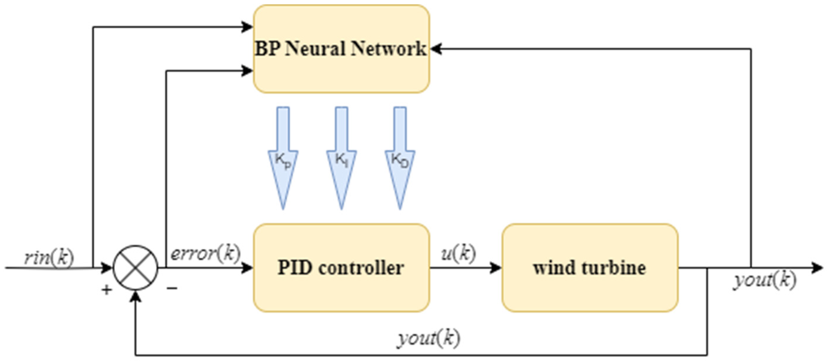
In general, traditional PID usually requires manual adjustment of parameters, so it cannot meet the demand for real-time tracking of wind power. In this paper, considering the uncertainty and randomness of wind power generation, traditional PID control exposes drawbacks such as a lack of adaptability and the need for manual tuning. Consequently, this paper proposes a BPNN-PID controller.

The BPNN-PID combines the self-learning capability of the BP neural network with the control ability of PID. By leveraging the feedback from the system, it can better utilize the difference between the practical output and the anticipated output. Through repetitive training using backpropagation, the network weights can be adaptively adjusted. As a result, the PID controller gains, which is capable of adapting to the unknown wind power generation, can be dynamically generated, leading to the real-time control of the system. The schematic structure of the BPNN-PID controller is illustrated in Figure 2.

2.2.1. Structure of the Wind Turbine Controller Based on BPNN-PID

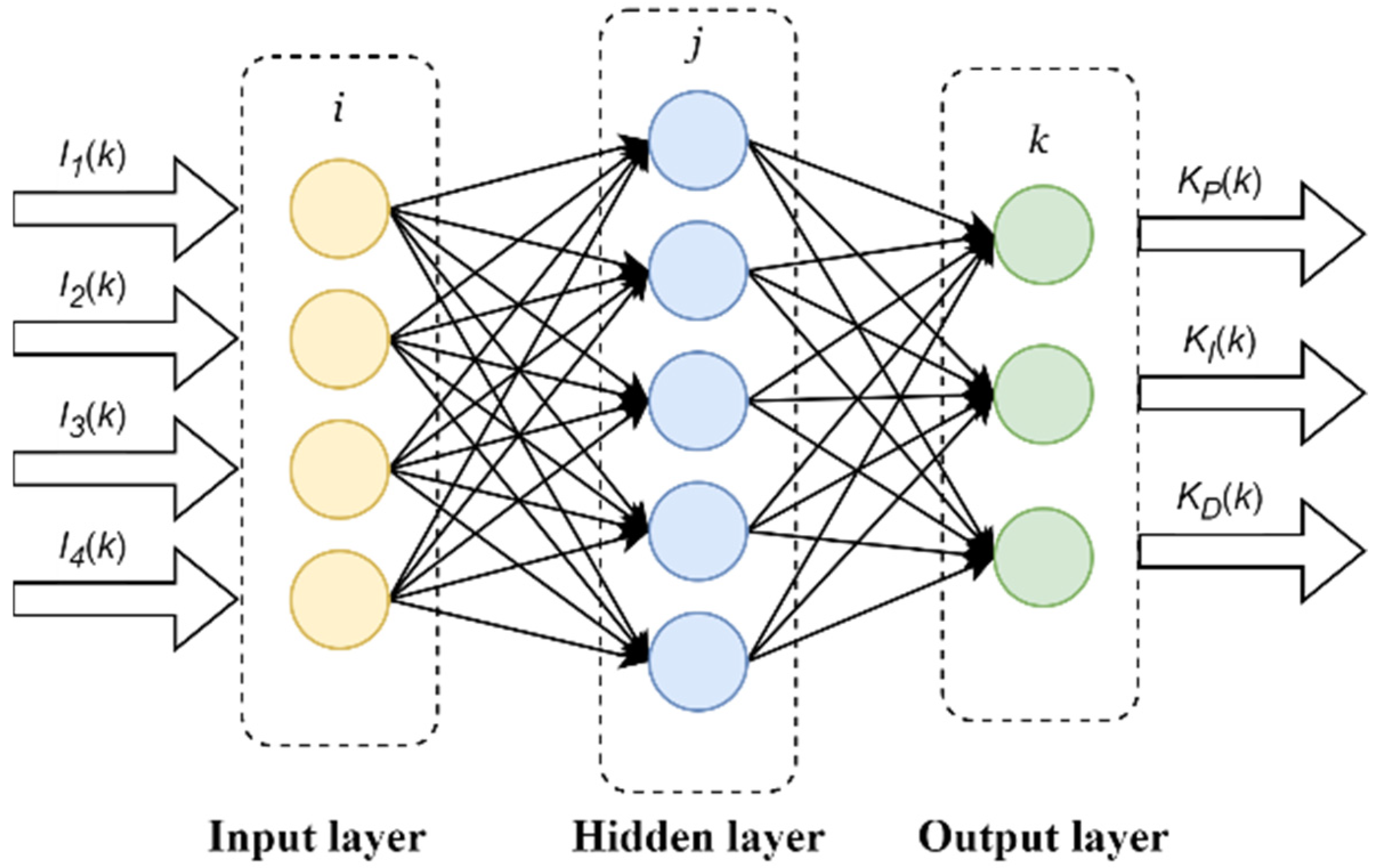
The quantity of hidden layers and neurons in BPNN determines the fitting and information processing capabilities of the network system [34,35,36,37]. The more complex the network, the stronger the fitting capability, but the training efficiency of data also reduces, leading to a decrease in the dynamic performance of wind turbine control [38,39]. After multiple attempts, this study ultimately employed a three-layer network to train PID gains, featuring four neurons in its input layer i, five neurons in its hidden layer j, and three neurons k in its output layer. The network’s structure is depicted in Figure 3.

The input of the network can be expressed by the following:

$$\left\{\begin{array}{l}{I}_1(k)=rin(k)\\ I_2(k)=yout(k)\\ I_3(k)=\mathrm{error}\left(k\right)=rin(k)-yout(k)\\ I_4(k)=1\end{array}\right.,$$

(10)

where rink(k) represents the wind turbine’s desired output power, yout(k) denotes the wind turbine’s actual output power, error(k) signifies the deviation in wind turbine output power, and the constant 1 serves to enhance the stability of the network.

BPNN provides output that aligns with the three gains of PID: K_P(k), K_I(k), and K_D(k).

The BPNN-PID controller’s output can be determined by utilizing the PID control gains derived from the network’s output in conjunction with the classical incremental PID control structure. This output can be expressed as follows:

$$u\left(k\right)=u\left(k-1\right)+\Delta u\left(k\right),$$

(11)

$$\begin{array}{l}\Delta u\left(k\right)=k_P\left(k\right)\left[error\left(k\right)-error\left(k-1\right)\right]+k_I\left(k\right)error\left(k\right)\\ +k_D\left(k\right)\left[error\left(k\right)-2error\left(k-1\right)-error\left(k-2\right)\right]\end{array},$$

(12)

where u(k) denotes the BPNN-PID controller’s output at time k, and Δu(k) represents the BPNN-PID controller’s output increment at time k.

2.2.2. Forward Propagation of BPNN-PID Control

Forward propagation is the inference stage in a neural network. It involves sequentially passing input data through the layers of the network in the forward direction, processing the data based on weights and activation functions, and ultimately outputting the PID gains. The specific details are as follows.

In the input layer, the i-th neuron’s output is the following:

$$O_i^{(1)}=I_i(k)(i=1,2,3,4)$$

(13)

The j-th neuron’s input to the hidden layer is obtained by weighting and summing the output of the input layer. The input to the j-th neuron in the hidden layer is the following:

$$ne{t}_j^{(2)}(k)={\displaystyle \sum _{i=1}^4{w}_{ij}^{(2)}(k)}{O}_i^{(1)}(k)(j=1,2,3,4,5),$$

(14)

where net_j⁽²⁾(k) represents the j-th neuron’s input in the hidden layer, and w_ij⁽²⁾(k) represents the weight parameter between input layer i and hidden layer j.

The output of the hidden layer can be obtained by processing the input through the activation function. The expression for the output of the j-th neuron in the hidden layer is represented by the following:

$$O_j^{(2)}(k)=f(ne{t}_j^{(2)}(k))(j=1,2,3,4,5),$$

(15)

$$f(x)=\tanh (x)={\displaystyle \frac{e^x-e^{-x}}{e^x+e^{-x}}},$$

(16)

where O_j⁽²⁾(k) represents the hidden layer’s output, f(x) represents the hidden layer’s activation function, and the tanh denotes the activation function. When the network has a shallow architecture, the tanh function is capable of achieving a balance between convergence accuracy and convergence speed.

The output of the hidden layer undergoes weighted summation to obtain the input to the k-th neuron in the output layer, as represented by the following:

$$ne{t}_k^{(3)}(k)={\displaystyle \sum _{j=1}^5{w}_{jk}^{(3)}(k)}{O}_j^{(2)}(k)(k=1,2,3),$$

(17)

where net_k⁽³⁾(k) represents the input to the k-th neuron in the output layer, and w_jk⁽³⁾(k) represents the weight parameter between output layer k and hidden layer j.

To obtain the output of the k-th neuron in the output layer using the activation function of the output layer, the k-th neuron’s output in the output layer can be expressed as follows:

$$O_{\mathrm{k}}^{(3)}(k)=g(ne{t}_k^{(3)}(k))(k=1,2,3),$$

(18)

$$g(x)=sigmoid(x)={\displaystyle \frac{1}{1+e^{-x}}},$$

(19)

where O_k⁽³⁾(k) represents the k-th neuro’s output in the output layer, and g(x) represents the activation function of the output layer. As the PID gains sought in this study were all within the range of 0–1, the sigmoid function was employed.

The output is explicitly represented as follows:

$$\left\{\begin{array}{l}{O}_1^{(3)}(k)=K_P(k)\\ O_2^{(3)}(k)=K_I(k)\\ O_3^{(3)}(k)=K_D(k)\end{array}\right.$$

(20)

2.2.3. Back Propagation of BPNN-PID Control

To mitigate the deviation between the actual power output and the intended power output of a wind power generation system, it is essential to select suitable performance evaluation criteria and propagate this criterion backward to update the network weights. Commonly, we opted for mean squared error as the evaluation criterion, that is,

$$\mathrm{error}(k)={\displaystyle \frac{1}{2}}{(\mathrm{rin}(k)-\mathrm{yout}(k))}^2$$

(21)

The error metric is propagated back through the network, utilizing the gradient descent method to compute the weight increment for each layer in the network and adjusting the network weights along the gradient direction. The updated weight parameters can train more suitable PID gains for the system, thereby effectively reducing the system error metric and improving system stability. The specific process of backpropagation is outlined below.

The combination of the error metric and the chain rule yields the weight increment for the k-th iteration, which is the following:

$$\Delta w_{jk}^{(3)}\left(k\right)=-\eta {\displaystyle \frac{\partial \mathrm{error}\left(k\right)}{\partial w_{jk}^{(3)}\left(k\right)}}+\alpha \Delta w_{jk}^{(3)}\left(k-1\right),$$

(22)

where η denotes the learning rate, and α represents the momentum factor. This session can enhance the speed of weight parameter correction and help avoid falling into local optima. According to the gradient descent policy, we can obtain the following:

$${\displaystyle \frac{\partial \mathrm{error}\left(k\right)}{\partial w_{jk}^{(3)}\left(k\right)}}={\displaystyle \frac{\partial \mathrm{error}\left(k\right)}{\partial yout\left(k\right)}}{\displaystyle \frac{\partial yout\left(k\right)}{\partial \Delta u\left(k\right)}}{\displaystyle \frac{\partial \Delta u\left(k\right)}{\partial O_k^{(3)}\left(k\right)}}{\displaystyle \frac{\partial O_k^{(3)}\left(k\right)}{\partial ne{t}_k^{(3)}\left(k\right)}}{\displaystyle \frac{\partial ne{t}_k^{(3)}\left(k\right)}{\partial w_{jk}^{(3)}\left(k\right)}},$$

(23)

where

$${\displaystyle \frac{\partial \mathrm{error}\left(k\right)}{\partial yout\left(k\right)}}=-\mathrm{error}\left(k\right),\left\{\begin{array}{l}{\displaystyle \frac{\partial \Delta u\left(k\right)}{\partial O_1^{(3)}\left(k\right)}}=error\left(k\right)-error\left(k-1\right)\\ {\displaystyle \frac{\partial \Delta u\left(k\right)}{\partial O_2^{(3)}\left(k\right)}}=error\left(k\right)\\ {\displaystyle \frac{\partial \Delta u\left(k\right)}{\partial O_3^{(3)}\left(k\right)}}=error\left(k\right)-2error\left(k-1\right)-error\left(k-2\right)\end{array}\right.$$

$${\displaystyle \frac{\partial O_k^{(3)}\left(k\right)}{\partial ne{t}_k^{(3)}\left(k\right)}}={\mathrm{g}}^{\prime }\left(\partial ne{t}_k^{(3)}\left(k\right)\right),{\displaystyle \frac{\partial ne{t}_k^{(3)}\left(k\right)}{\partial w_{jk}^{(3)}\left(k\right)}}=O_j^{(2)}\left(k\right),{\displaystyle \frac{\partial yout\left(k\right)}{\partial \Delta u\left(k\right)}}=\mathrm{sgn}\left({\displaystyle \frac{\partial yout\left(k\right)}{\partial \Delta u\left(k\right)}}\right)$$

(24)

Based on the above derivation, the weight increment can be expressed as follows:

$$\Delta w_{jk}^{(3)}\left(k\right)=\eta d_k^{(3)}\left(k\right)O_j^{(2)}\left(k\right)+\alpha \Delta w_{jk}^{(3)}\left(k-1\right),$$

(25)

where d_k⁽³⁾ is the output layer error:

$$d_k^{(3)}=-\mathrm{error}\left(k\right)\mathrm{sgn}\left({\displaystyle \frac{\partial yout\left(k\right)}{\partial \Delta u\left(k\right)}}\right){\displaystyle \frac{\partial \Delta u\left(k\right)}{\partial O_k^{(3)}\left(k\right)}} {\mathrm{g}}^{\prime }\left(\partial ne{t}_k^{(3)}\left(k\right)\right)$$

(26)

$${\mathrm{g}}^{\prime }\left(x\right)=\mathrm{g}\left(x\right)\left(1-\mathrm{g}\left(x\right)\right)$$

(27)

Similarly, the weight increment from the input layer to the hidden layer for the k-th iteration is given by the following:

$$\Delta w_{jk}^{(3)}\left(k\right)=\eta d_j^{(2)}\left(k\right)O_i^{(1)}\left(k\right)+\alpha \Delta w_{ij}^{(2)}\left(k-1\right),$$

(28)

where d_j⁽²⁾(k) is the hidden layer error:

$$d_j^{(2)}\left(k\right)=f^{\prime }\left(ne{t}_j^{(2)}\left(k\right)\right){\displaystyle \sum _{j=1}^5{d}_k^{(3)}(k)w_{jk}^{(3)}\left(k\right)}$$

(29)

$$f^{\prime }\left(x\right)=1-f^2\left(x\right)$$

(30)

2.3. Thermal Plant Modelling

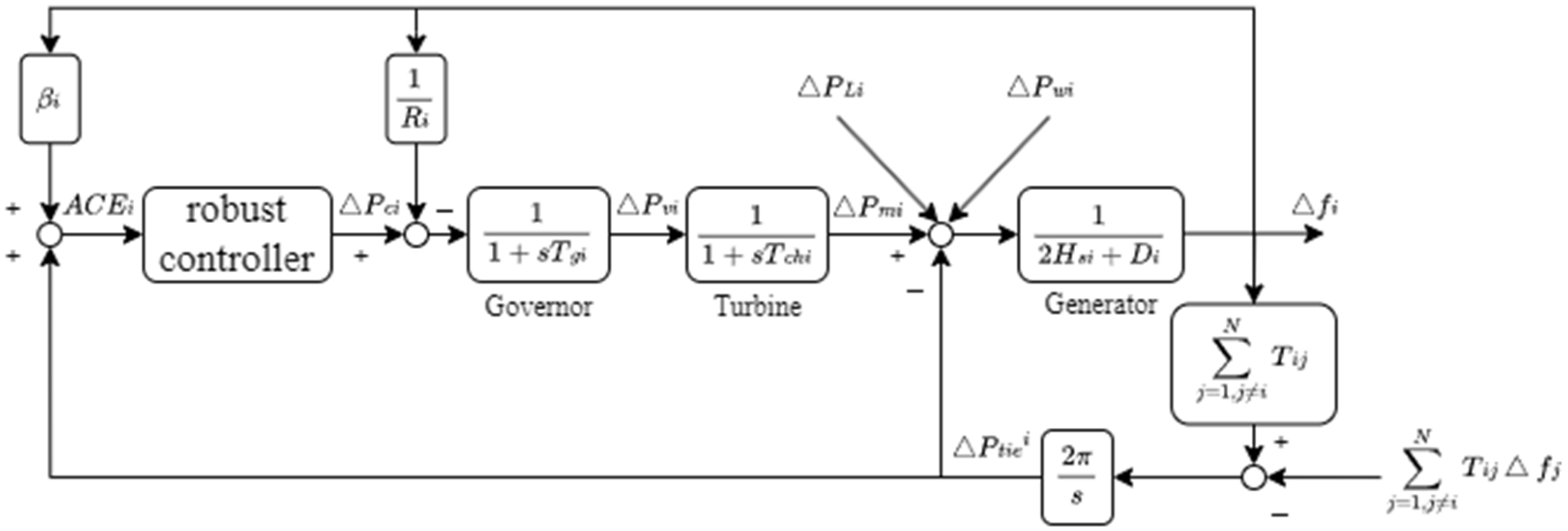
A typical interconnected power system typically involves multiple areas physically connected by tie-lines. As depicted in Figure 4, a multi-area power system model is illustrated. To facilitate the robust control strategy derivation, the frequency response model of each area is equivalently represented as an aggregated generator unit, load, and wind turbine. Within each control area, the dynamics consist of the following five components.

The turbine dynamics are depicted as follows:

$$\Delta {\stackrel{•}{P}}_{mi}=\left(-{\displaystyle \frac{1}{T_{Ti}}}\right)\Delta P_{mi}+\left({\displaystyle \frac{1}{T_{Ti}}}\right)\Delta P_{vi},$$

(31)

where ΔP_mi is the generator mechanical power deviation of area i, ΔP_vi is the turbine valve position deviation of area i, and T_Ti is the time constant of turbine i.

The governor is characterized by the following:

$$\Delta {\stackrel{•}{P}}_{vi}=\left(-{\displaystyle \frac{1}{R_i{T}_{gi}}}\right)\Delta f_i+\left(-{\displaystyle \frac{1}{T_{gi}}}\right)\Delta P_{vi}+\left({\displaystyle \frac{1}{T_{gi}}}\right)\Delta P_{ci},$$

(32)

where R_i represents the speed droop coefficient of area i, ΔP_ci represents the supplementary control action of area i, and T_gi represents the time constant of governor i.

The area frequency deviation indirectly reflects the relationship between the generator setpoint and the load demand; this relationship can be represented by the following:

$$\Delta {\stackrel{•}{f}}_i=\left({\displaystyle \frac{1}{2H_i}}\right)\Delta P_{mi}+\left(-{\displaystyle \frac{D_i}{2H_i}}\right)\Delta f_i+\left(-{\displaystyle \frac{1}{2H_i}}\right)\Delta P_{tie,i}+\left(-{\displaystyle \frac{1}{2H_i}}\right)\Delta P_{wi}+\left(-{\displaystyle \frac{1}{2H_i}}\right)\Delta P_{Li},$$

(33)

where Δf_i represents the frequency deviation of area i, ΔP_tie,i represents the inter-area tie-line power flow deviation, ΔP_wi represents the wind power output of wind turbine i, ΔP_Li represents the non-frequency-sensitive load change of area i, H_i represents the inertia constant of generator i, and D_i represents the load-damping constant of area i.

The inter-area tie-line power flow deviation is represented as follows:

$$\Delta {\stackrel{•}{P}}_{tie,i}=2\pi {\displaystyle \sum _{j=1,j\ne i}^N{T}_{ij}\left(\Delta f_i-\Delta f_j\right)},$$

(34)

where T_ij represents the Synchronized Control Variables, and Δf_j is the deviation of frequency within area j.

For a MAPS, it is crucial to maintain the regional frequency deviation within a specified range by adjusting the active power flow through tie-lines. Therefore, the Area Control Error (ACE) is usually introduced. The ACE is formulated as the weighted sum of regional frequency deviations and tie-line power deviations, which is expressed by the following:

$$AC{E}_i=P_{tie,i}+{\beta }_i\Delta f_i,$$

(35)

$${\beta }_i={\displaystyle \frac{1}{R_i}}+D_i,$$

(36)

where β_i is the frequency deviation coefficient.

According to the above analysis, the state-space representation of a multi-area interconnected power system can be depicted as follows:

$$\left\{\begin{array}{l}{\dot{x}}_i={\mathcal{A}}_i{x}_i+{\displaystyle \sum _{j=1,j\ne i}^N{\mathcal{A}}_{ij}{x}_j}+{\mathcal{B}}_i{u}_i+{\mathcal{F}}_i{w}_i\\ y_i={\mathcal{C}}_{1i}{x}_i\\ z_i={\mathcal{E}}_{2i}{x}_i\end{array}\right.,$$

(37)

where x_i represents the state vector of area i within the system, u_i represents the output of the controller for the area i, w_i represents the disturbance magnitude within the area i, y_i represents the output of the system in area i, and z_i represents the quantity that we are interested in to facilitate the robust performance index incorporation.

$$x_i={[\Delta P_{mi} \Delta f_i \Delta P_{vi} \Delta P_{tie}^i {\displaystyle \int AC{E}_i}]}^T,w_i=\Delta P_{Li}+\Delta P_{wi}$$

$$\begin{array}{l}{\mathcal{A}}_i=\left[\begin{array}{ccccc}{\displaystyle \frac{-1}{T_{Ti}}}& 0& {\displaystyle \frac{1}{T_{Ti}}}& 0& 0\\ {\displaystyle \frac{1}{2H_i}}& {\displaystyle \frac{-{\mathcal{D}}_i}{2H_i}}& 0& {\displaystyle \frac{-1}{2H_i}}& 0\\ 0& {\displaystyle \frac{-1}{R_i{T}_{gi}}}& {\displaystyle \frac{-1}{T_{gi}}}& 0& 0\\ 0& 2\pi {\displaystyle \sum _{j=1,j\ne i}^N{T}_{ij}}& 0& 0& 0\\ 0& {\beta }_i& 0& 1& 0\end{array}\right],\\ {\mathcal{A}}_{ij}=\left[\begin{array}{ccccc}0& 0& 0& 0& 0\\ 0& 0& 0& 0& 0\\ 0& 0& 0& 0& 0\\ 0& 2\pi {\displaystyle \sum _{j=1,j\ne i}^N{T}_{ij}}& 0& 0& 0\\ 0& 0& 0& 0& 0\end{array}\right],\\ {\mathcal{B}}_i=\left[\begin{array}{c}0\\ 0\\ {\displaystyle \frac{1}{T_{gi}}}\\ 0\\ 0\end{array}\right],{\mathcal{F}}_i=\left[\begin{array}{c}0\\ {\displaystyle \frac{-1}{2H_i}}\\ 0\\ 0\\ 0\end{array}\right],{\mathcal{C}}_i={\left[\begin{array}{cc}0& 0\\ {\beta }_i& 0\\ 0& 0\\ 1& 0\\ 0& 1\end{array}\right]}^T,{\mathcal{E}}_i=\left[\begin{array}{c}0\\ 1\\ 0\\ 0\\ 0\end{array}\right]\end{array}$$

Due to the fact that the state measurements are collected from digital sensors, e.g., Phasor Measurement Units and Remote Telemetry Units, the discrete-time LFC model is given as follows:

$$\left\{\begin{array}{l}{\dot{x}}_i\left(k+1\right)=A_i{x}_i\left(k\right)+{\displaystyle \sum _{j=1,j\ne i}^N{A}_{ij}{x}_j}\left(k\right)+B_i{u}_i\left(k\right)+F_i{w}_i\left(k\right)\\ y_i\left(k\right)=C_i{x}_i\left(k\right)\\ z_i\left(k\right)=E_i{x}_i\left(k\right)\end{array}\right.,$$

(38)

where

$$A_i=e^{{\mathcal{A}}_{i}h},B_i={\displaystyle \underset{0}{\overset{h}{\int }}{e}^{{\mathcal{A}}_{i}h}{\mathcal{B}}_{i}dt},F_i={\displaystyle \underset{0}{\overset{h}{\int }}{e}^{{\mathcal{A}}_{i}h}{\mathcal{F}}_{i}dt},C_i={\mathcal{C}}_i,E_i={\mathcal{E}}_i,$$

and h represents the sampling period.

2.4. Robust LFC with Wind Turbine Power Penetration

The integration of wind power into a MAPS aggravates the system imbalance between load and demand, and after the wind power is suppressed, its fluctuation is still large compared with the load fluctuation. Therefore, considering the mutual influence of interconnected regions, this paper introduces control gains for regions i and its neighbor j and designed a robust distributed output feedback controller, which is the following:

$$u_i\left(\mathrm{k}\right)=G_i{y}_i\left(k\right)+{\displaystyle \sum _{j=1,j\ne i}^N{G}_{ij}{y}_j\left(k\right)},$$

(39)

where G_i represents the local control gain of region i, and G_ij denotes the neighboring control gains corresponding to area j.

The closed-loop LFC model is, therefore, represented by the following:

$${\dot{x}}_i\left(k+1\right)=\left(A_i+B_i{G}_i{C}_i\right)x_i\left(k\right)+{\displaystyle \sum _{j=1,j\ne i}^N\left(B_i{G}_{ij}{C}_j+A_{ij}\right)x_j}\left(k\right)+F_i{w}_i\left(k\right)$$

(40)

In order to determine the gains G_i and G_ij, the following two theorems are deduced.

Theorem 1.

The existence of a matrix Q_i > 0 i = 1,2,3…N is such that it renders the MAPS asymptotically stable while ensuring that the frequency deviations meet the expected H_∞ performance index γ. The matrix Q_i satisfies the following constraints:

$$\left[\begin{array}{cc}{\overline{A}}^{T}Q\overline{A}+E{E}^T-Q& {\overline{A}}^{T}QE\\ *& F^{T}QF-{\gamma }^{2}I\end{array}\right]<0 ,$$

(41)

where

$$\begin{gathered} \overline{A}=A+BGC,B=\mathrm{diag}\left\{B_1,B_2\dots B_N\right\},E=\mathrm{diag}\left\{E_1,E_2\dots E_N\right\}C=\mathrm{diag}\left\{C_1,C_2\dots C_N\right\}, \\ F=\mathrm{diag}\left\{F_1,F_2\dots F_N\right\},Q=\mathrm{diag}\left\{Q_1,Q_2\dots Q_N\right\}, \\ A=\left[\begin{array}{cccc}{A}_{11}& A_{12}& \cdots & A_{1N}\\ A_{21}& A_{22}& \cdots & A_{2N}\\ ⋮& ⋮& \ddots & ⋮\\ A_{N1}& A_{N2}& \cdots & A_{NN}\end{array}\right],A=\left[\begin{array}{cccc}{A}_{11}& A_{12}& \cdots & A_{1N}\\ A_{21}& A_{22}& \cdots & A_{2N}\\ ⋮& ⋮& \ddots & ⋮\\ A_{N1}& A_{N2}& \cdots & A_{NN}\end{array}\right] \end{gathered}$$

Under zero initial conditions, γ satisfies the following definition.

$${‖\Delta f_i‖}_2^2<{\eta }^2{‖w_i‖}_2^2 \forall 0\ne w_i\in \left[0,\infty \right),$$

(42)

where

$${‖\Delta f_i‖}_2=\sqrt{{\displaystyle \sum _{k=0}^{\infty }\Delta f_i^T\left(k\right)}\Delta f_i\left(k\right)},{‖w_i‖}_2=\sqrt{{\displaystyle \sum _{k=0}^{\infty }{w}_i^T\left(k\right)}{w}_i\left(k\right)}$$

(43)

Since the regional control gains G_i and G_ij cannot be directly obtained using the MATLAB LMI toolbox, the matrix transformation technique is employed for the solution. The derived sufficient LMI condition is presented in Theorem 2.

Theorem 2.

The existence of a matrix Q_i > 0 i = 1, 2, 3…N, matrix R is such that it renders the MAPS asymptotically stable while ensuring that the frequency deviations meet the expected H_∞ performance index γ, and the regional control gain G = (QB)^☆RC^☆. The matrix Q_i and matrix R satisfies the following constraints:

$$\left[\begin{array}{ccc}-Q& QA+R& QF\\ *& E{E}^T-Q& 0\\ *& *& -{\gamma }^{2}I\end{array}\right]<0,$$

(44)

where ☆ represents the corresponding pseudo-inverse matrices. To refer to the proof process, please consult reference [40].

3. Results

3.1. System Structure and Parameters

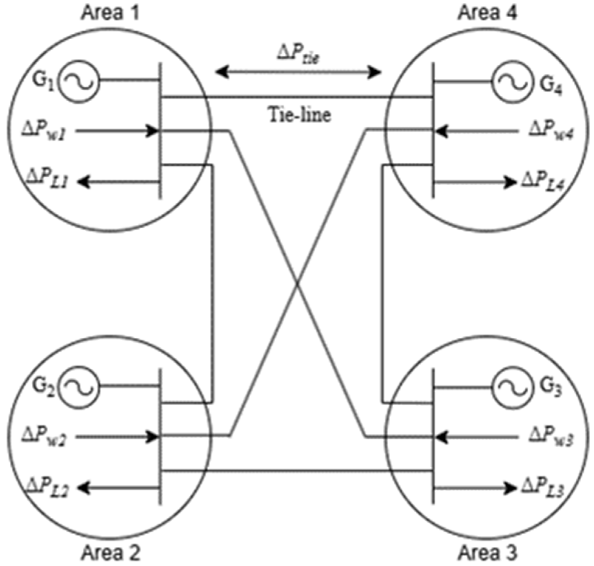
In order to verify the effectiveness of the control strategy proposed in this paper, this section takes the four-region interconnected power system as the framework for verification. In the verification, the operating point of the wind turbine was set at 247 MW, and the wind speed was fixed at 11 m/s. The structure of the four-area power system is shown in Figure 5, and

Table 1. Power system parameters for each area.

Area 1	Area 2	Area 3	Area 4
D1 = 0.4	D2 = 1	D3 = 0.8	D4 = 0.5
2H1 = 10	2H2 = 12	2H3 = 15	2H4 = 13
Tch1 = 1.6	Tch2 = 1.2	Tch3 = 1.9	Tch4 = 1.4
Tg1 = 0.7	Tg2 = 0.9	Tg3 = 0.5	Tg4 = 0.8
R1 = 0.04	R2 = 0.06	R3 = 0.08	R4 = 0.05
T12 = 0.04	T21 = 0.04	T31 = 0	T41 = 0.12
T13 = 0	T23 = 0.08	T32 = 0.08	T42 = 0.1
T14 = 0.12	T24 = 0.1	T34 = 0.2	T43 = 0.2

and

Table 2. Wind turbine system parameters.

ωs	Rr	Rs	Ls	Lm	Lr	Ht
1.17	0.00552	0.00491	0.09273	3.9654	0.1	4.5

show the parameters of the power system and wind turbines in the four areas. The specific structure and system parameters can refer to the literature [40].

3.2. Validations on BPNN-Based PID Control for Wind Turbine

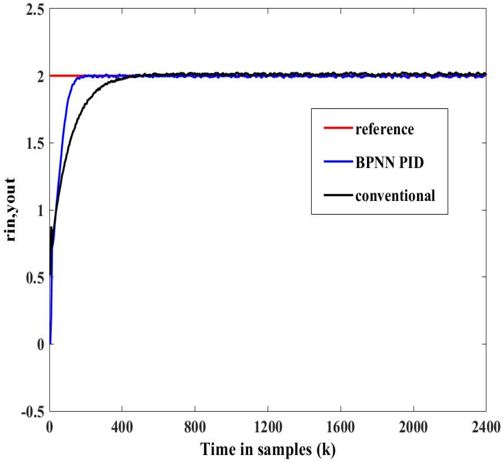
Figure 6 depicts the tracking performance of the conventional PID controller and the BPNN-PID controller on rated wind power harvesting. A comparative analysis reveals that BPNN-PID exhibits a faster response compared with traditional PID control. Therefore, the rapid power response achieved through BPNN-PID can effectively alleviate the impact of wind power fluctuations on the multi-area interconnected power system.

Figure 7 illustrates the variation in gains for BPNN-PID, and conventional PID controller gain is a fixed experience value. Compared with the fixed gains in traditional PID control, it is evident that the gains of the BPNN-PID controller dynamically track the power variations in the wind power system. The controller adaptively solves gains in response to varying wind power fluctuations.

3.3. Robust Validations on LFC with Wind Turbine Integration

Because the larger power fluctuations caused by the integrated wind farm compared with the regional load disturbances, this significant power fluctuation can impact the power system. Therefore, we aim to verify the effectiveness of the proposed robust controller and examine whether the regional frequency deviations satisfy the H_∞ performance criterion.

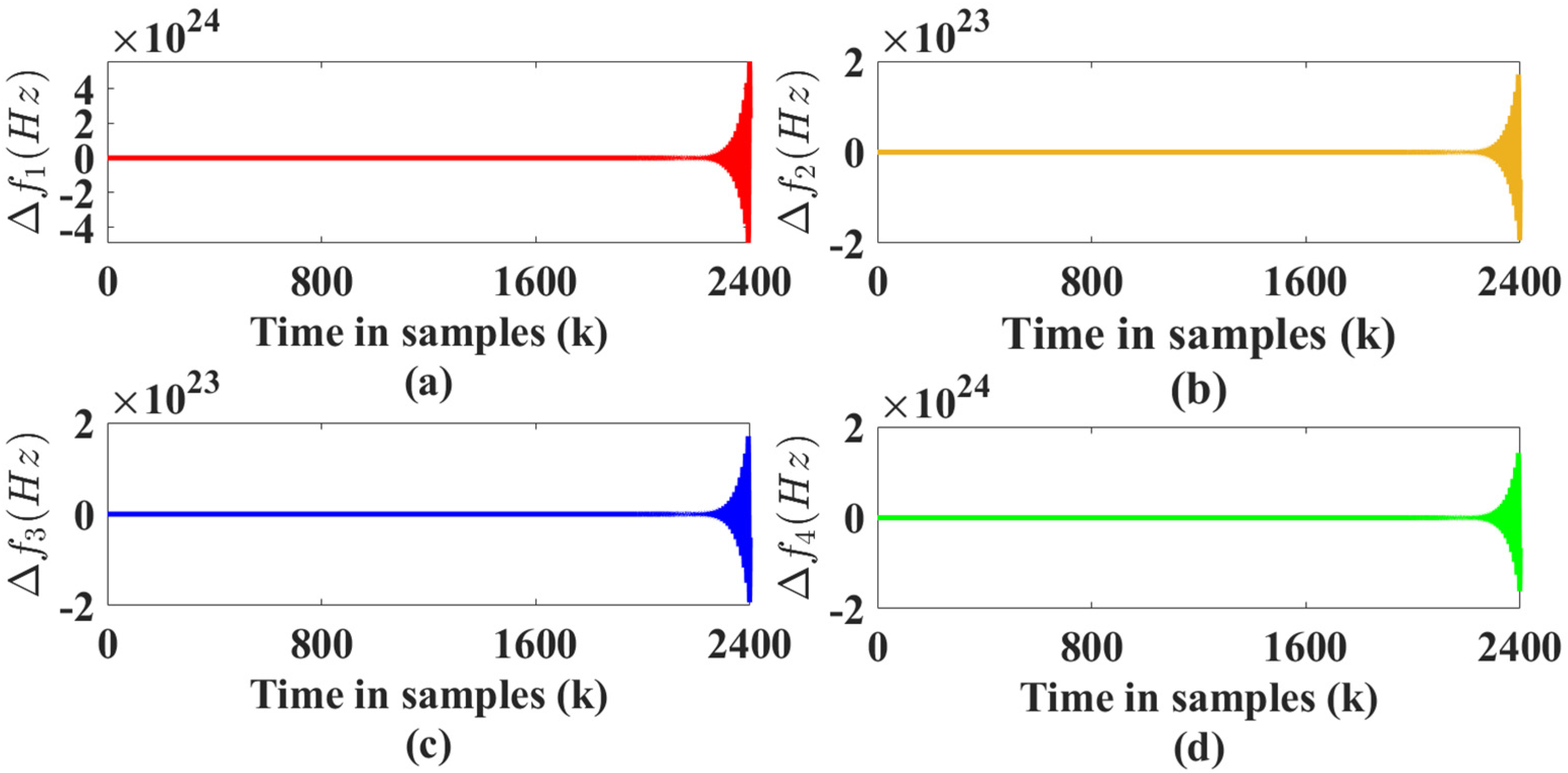
Figure 8 depicts the dynamic frequency deviations of the four regions in an open-loop state. With the system operation time increasing, the regional frequency deviations of the system diverge, leading to system instability. The feasibility of integrating the wind farm into the grid is compromised.

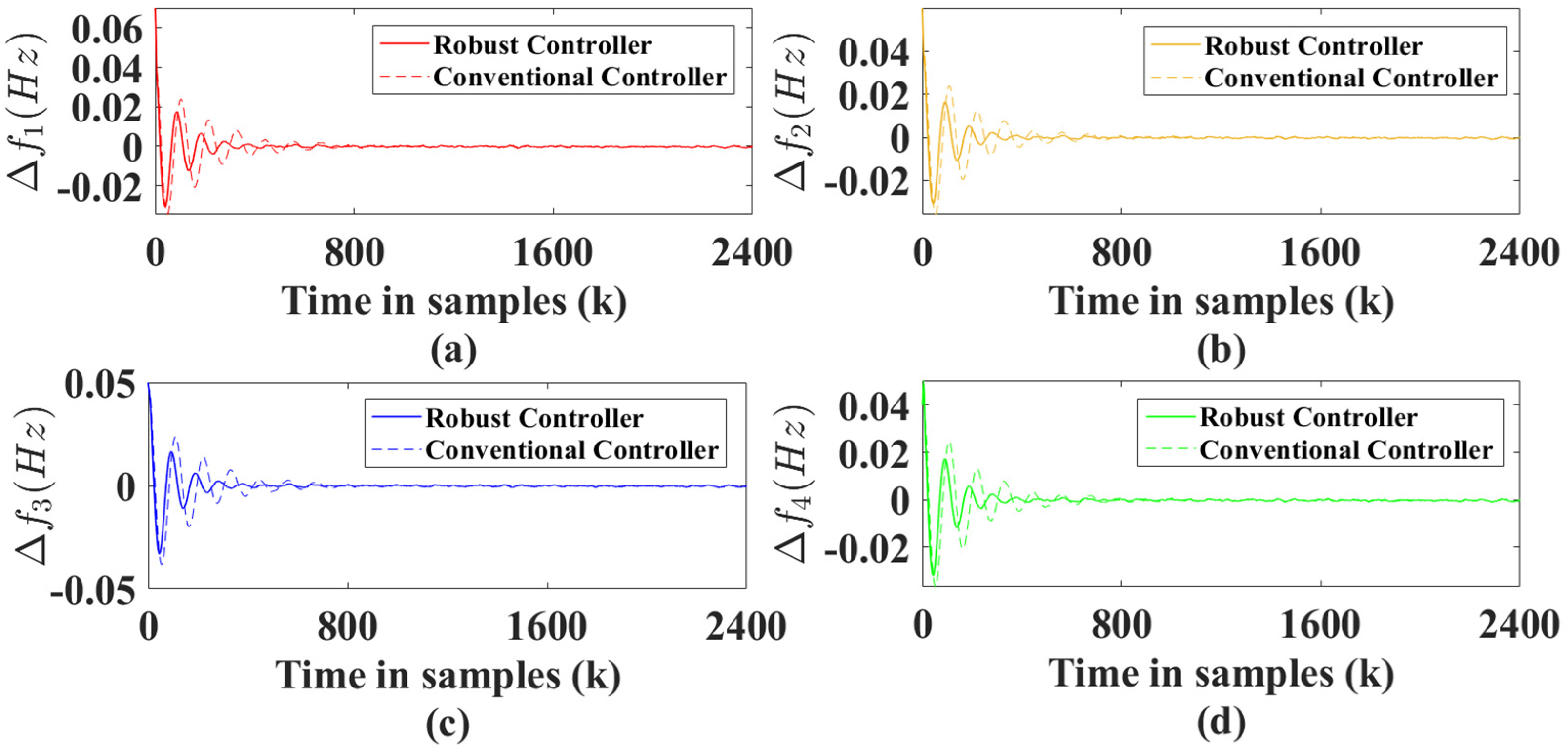
To demonstrate the efficacy of the robust controller, we conducted a comparison between the proposed robust controller and a conventional controller. Figure 9 illustrates the frequency response characteristics of the four areas in the closed-loop system. In comparison to Figure 8, it is evident that, under the fast response of the regional controller, the frequency deviations of the four regions converge rapidly. In Figure 9, the proposed robust controller in this study exhibits a faster convergence rate compared with the traditional LFC controller. It effectively mitigates the impact of wind power and load fluctuations on the system, ensuring that regional frequency deviations meet the H_∞ performance criterion. This validates the feasibility of the proposed robust controller in a MAPS with an integrated wind farm.

Figure 10 illustrates the dynamic of tie-line power. Under the fast response of the regional controller, the power exchange between the four regions converges rapidly. Additionally, it is observable that the robust controller presented in this study exhibits a faster convergence rate compared with the traditional LFC controller. Therefore, the proposed robust controller not only outperforms the traditional LFC controller in terms of regional frequency error response but also demonstrates effective control over inter-area power exchange. This validates the applicability of the proposed robust controller in systems considering both intra-regional disturbances and inter-area influences.

4. Conclusions

The BPNN-PID controller proposed in this paper can respond to wind power fluctuations quickly and deal with the pressure of large-scale wind power integration more quickly and accurately than the traditional controller. Furthermore, simulation results demonstrated that after the initial adjustment of the BPNN controller, the combination of robust controllers could make the frequency of the whole four-region power system more stable and reach the H_∞ performance criteria. Compared with the traditional robust controller, the robust controller can make the frequency convergence of each region faster. In the future, we hope to focus on solving the problem of sustainable energy control through machine learning so as to improve the multi-regional frequency.

References

1. Renewables. Available online: www.iea.org/energy-system/renewables (accessed on 20 June 2024).
2. Gayen, D.; Chatterjee, R.; Roy, S. A review on environmental impacts of renewable energy for sustainable development. Int. J. Environ. Sci. Technol. 2024, 21, 5285–5310. [Google Scholar] [CrossRef]
3. Hanwate, S.; Hote, Y.V.; Saxena, S. Adaptive policy for load frequency control. IEEE Trans. Power Syst. 2017, 33, 1142–1144. [Google Scholar] [CrossRef]
4. Chen, C.; Zhang, K.; Geng, J.; Yuan, K.; Yang, Z.; Li, L. Multiobjective-based optimal allocation scheme for load frequency control. Int. Trans. Electr. Energy Syst. 2017, 27, e2334. [Google Scholar] [CrossRef]
5. Fan, Q.; Wang, X.; Yuan, J.; Liu, X.; Hu, H.; Lin, P. A review of the development of key technologies for offshore wind power in China. J. Mar. Sci. Eng. 2022, 10, 929. [Google Scholar] [CrossRef]
6. Neya, N.M.; Saberi, S.; Rezaie, B. Design of an adaptive controller to capture maximum power from a variable speed wind turbine system without any prior knowledge of system parameters. Trans. Inst. Meas. Control 2022, 44, 609–619. [Google Scholar] [CrossRef]
7. Wang, Y.; Guan, Y.; Li, H.; Chen, M. Spiking-free disturbance observer-based fixed-time sliding mode control of maximum power extraction from wind turbine. Trans. Inst. Meas. Control 2024, 46, 555–565. [Google Scholar] [CrossRef]
8. Mahvash, H.; Taher, S.A.; Rahimi, M.; Shahidehpour, M. Enhancement of DFIG performance at high wind speed using fractional order PI controller in pitch compensation loop. Int. J. Electr. Power Energy Syst. 2019, 104, 259–268. [Google Scholar] [CrossRef]
9. Mahvash, H.; Taher, S.A.; Shahidehpour, M. Fractional order control scheme in pitch control loop of synchronous generator wind turbine type 4 at high wind speed operation in a microgrid. J. Renew. Sustain. Energy 2019, 11, 013305. [Google Scholar] [CrossRef]
10. Varzaneh, S.G.; Gharehpetian, G.B.; Abedi, M. Output power smoothing of variable speed wind farms using rotor-inertia. Electr. Power Syst. Res. 2014, 116, 208–217. [Google Scholar] [CrossRef]
11. Bernard, M.Z.; Mohamed, T.H.; Ali, R.; Mitani, Y.; Qudaih, Y.S. PI-MPC frequency control of power system in the presence of DFIG wind turbines. Engineering 2013, 5, 43. [Google Scholar] [CrossRef]
12. Chapaloglou, S.; Varagnolo, D.; Marra, F.; Tedeschi, E. Data-driven energy management of isolated power systems under rapidly varying operating conditions. Appl. Energy 2022, 314, 118906. [Google Scholar] [CrossRef]
13. Qian, D.; Fan, G. Neural-network-based terminal sliding mode control for frequency stabilization of renewable power systems. IEEE/CAA J. Autom. Sin. 2018, 5, 706–717. [Google Scholar] [CrossRef]
14. Iqbal, A.; Ying, D.; Saleem, A.; Hayat, M.A.; Mateen, M. Proposed particle swarm optimization technique for the wind turbine control system. Meas. Control 2020, 53, 1022–1030. [Google Scholar] [CrossRef]
15. Deng, Z.; Xu, Y.; Gu, W.; Fei, Z. Finite-time convergence robust control of battery energy storage system to mitigate wind power fluctuations. Int. J. Electr. Power Energy Syst. 2017, 91, 144–154. [Google Scholar] [CrossRef]
16. Zhang, X.; Gu, J.; Hua, L.; Ma, K. Enhancing performances on wind power fluctuation mitigation by optimizing operation schedule of battery energy storage systems with considerations of operation cost. IEEE Access 2019, 7, 94072–94083. [Google Scholar] [CrossRef]
17. Alam, M.J.E.; Muttaqi, K.M.; Sutanto, D. Battery energy storage to mitigate rapid voltage/power fluctuations in power grids due to fast variations of solar/wind outputs. IEEE Access 2021, 9, 12191–12202. [Google Scholar] [CrossRef]
18. Ma, D.; Niculescu, S.; Guo, L.; Chen, J. Special issue on PID control in the information age: Theoretical advances and applications. Int. J. Robust Nonlinear Control 2022, 32, 9384–9388. [Google Scholar] [CrossRef]
19. Indulkar, C.; Raj, B. Application of fuzzy controller to automatic generation control. Electr. Mach. Power Syst. 1995, 23, 209–220. [Google Scholar] [CrossRef]
20. Karnavas, Y.; Papadopoulos, D. AGC for autonomous power system using combined intelligent techniques. Electr. Power Syst. Res. 2002, 62, 225–239. [Google Scholar] [CrossRef]
21. Ramakrishna, K.; Bhatti, T. Discrete data load frequency control of two-area power system with multi-source power generation. Int. Energy J. 2008, 9, 145–154. [Google Scholar]
22. Hu, Z.; Liu, S.; Luo, W.; Wu, L. Intrusion-detector-dependent distributed economic model predictive control for load frequency regulation with PEVs under cyber attacks. IEEE Trans. Circuits Syst. I Regul. Pap. 2021, 68, 3857–3868. [Google Scholar] [CrossRef]
23. Hu, Z.; Zhang, K.; Su, R. Robust Cooperative Load Frequency Control for Enhancing Wind Energy Integration in Multi-Area Power Systems. IEEE Trans. Autom. Sci. Eng. 2024, 1–11. [Google Scholar] [CrossRef]
24. Hu, Z.; Su, R.; Wang, R. Robust Distributed Load Frequency Control for Multi-Area Wind Energy-Dominated Microgrids Considering Phasor Measurement Unit Failures. IEEE Internet Things J. 2024, 11, 23475–23484. [Google Scholar] [CrossRef]
25. Hu, Z.; Liu, S.; Luo, W.; Wu, L. Resilient distributed fuzzy load frequency regulation for power systems under cross-layer random denial-of-service attacks. IEEE Trans. Cybern. 2022, 52, 2396–2406. [Google Scholar] [CrossRef]
26. Ancuti, M.-C.; Musuroi, S.; Sorandaru, C.; Dordescu, M.; Erdodi, G.M. Wind turbines optimal operation at time variable wind speeds. Appl. Sci. 2020, 10, 4232. [Google Scholar] [CrossRef]
27. Yin, X.; Zhang, W.; Zhao, X. Current status and future prospects of continuously variable speed wind turbines: A systematic review. Mech. Syst. Signal Process. 2019, 120, 326–340. [Google Scholar] [CrossRef]
28. Li, D.; Sang, Y.; Fang, S.; Sun, C.; Wang, H. Wind tunnel test research on the aerodynamic behavior of concrete-filled double-skin steel (CFDST) wind turbine towers. Buildings 2024, 14, 2372. [Google Scholar] [CrossRef]
29. Li, D.; Zhang, Z.; Zhou, X.; Zhang, Z.; Yang, X. Cross-wind dynamic response of concrete-filled double-skin wind turbine towers: Theoretical modelling and experimental investigation. J. Vib. Control 2023, 30, 2881–2893. [Google Scholar] [CrossRef]
30. Bedoud, K.; Rhif, A.; Bahi, T.; Merabet, H. Study of a double fed induction generator using matrix converter: Case of wind energy conversion system. Int. J. Hydrog. Energy 2018, 43, 11432–11441. [Google Scholar] [CrossRef]
31. Ekanayake, J.; Jenkins, N.; Strbac, G. Frequency response from wind turbines. Wind. Eng. 2008, 32, 573–586. [Google Scholar] [CrossRef]
32. Garrido, J.; Ruz, M.L.; Morilla, F.; Vázquez, F. Interactive tool for frequency domain tuning of PID controllers. Processes 2018, 6, 197. [Google Scholar] [CrossRef]
33. Son, Y.-D.; Bin, S.-D.; Jin, G.-G. Stability Analysis of a Nonlinear PID Controller. Int. J. Control Autom. Syst. 2021, 19, 3400–3408. [Google Scholar] [CrossRef]
34. Dey, R.; Dhar, R.S.; Mondal, U. Artificial neural network–based modelling of pacemaker and its pace tracking using discrete wavelet transform–based finite dimension repetitive controller. Trans. Inst. Meas. Control 2024, 46, 1410–1417. [Google Scholar] [CrossRef]
35. Yu, T.; Liu, J.; Zeng, Y.; Zhang, X.; Zeng, Q.; Wu, L. Stability analysis of genetic regulatory networks with switching parameters and time delays. IEEE Trans. Neural Netw. Learn. Syst. 2017, 29, 3047–3058. [Google Scholar] [CrossRef]
36. Wang, M.; Chen, J.; Wen, C.; Qin, S. Adaptive generalized Nash equilibrium seeking algorithm for non-smooth aggregative game under dynamic event-triggered mechanism. Automatica 2024, 169, 111835. [Google Scholar] [CrossRef]
37. Wang, M.; Wu, Y.; Qi, S. Generalized Nash equilibrium seeking for noncooperative game with different monotonicity by adaptive neurodynamic algorithm. IEEE Trans. Neural Netw. Learn. Syst. 2024, 95, 266–272. [Google Scholar] [CrossRef]
38. Wang, L.; Ye, W.; Zhu, Y.; Yang, F.; Zhou, Y. Optimal parameters selection of back propagation algorithm in the feedforward neural network. Eng. Anal. Bound. Elem. 2023, 151, 575–596. [Google Scholar] [CrossRef]
39. Wu, Y.; Feng, J. Development and application of artificial neural network. Wirel. Pers. Commun. 2018, 102, 1645–1656. [Google Scholar] [CrossRef]
40. Hu, Z.; Su, R.; Ling, K.-V.; Guo, Y.; Ma, R. Resilient event-triggered MPC for load frequency regulation with wind turbines under false data injection attacks. IEEE Trans. Autom. Sci. Eng. 2023, 1–11. [Google Scholar] [CrossRef]
Figure 1. Wind power system structure diagram.
Sustainability 16 08062 g001
Figure 2. BPNN-PID structure diagram.
Sustainability 16 08062 g002
Figure 3. BPNN structure diagram.
Sustainability 16 08062 g003
Figure 4. Regional control model for area i.
Sustainability 16 08062 g004
Figure 5. Four-area power system topology.
Sustainability 16 08062 g005
Figure 6. Comparison graph of wind power tracking.
Sustainability 16 08062 g006
Figure 7. BPNN-PID gain. (a) KP; (b) KI; (c) KD.
Sustainability 16 08062 g007
Figure 8. Dynamic changes in the open-loop system frequency. (a) f 1 ; (b) f 2 ; (c) f 3 ; (d) f 4 .
Sustainability 16 08062 g008
Figure 9. Dynamic changes in frequency with robust controller. (a) f 1 ; (b) f 2 ; (c) f 3 ; (d) f 4 .
Sustainability 16 08062 g009
Figure 10. Dynamic changes in inter-area power exchange with robust controller. (a) P t i e 1 ; (b) P t i e 2 ; (c) P t i e 3 ; (d) P t i e 4 .
Sustainability 16 08062 g010