Abstract
Amidst the accelerating growth of intelligent power systems, the integrity of vast and complex datasets has become essential to promoting sustainable energy management, ensuring energy security, and supporting green living initiatives. This study introduces a novel hybrid machine learning model to address the critical issue of missing power load data—a problem that, if not managed effectively, can compromise the stability and sustainability of power grids. By integrating meteorological and temporal characteristics, the model enhances the precision of data imputation by combining random forest (RF), Spearman weighted k-nearest neighbors (SW-KNN), and Levenberg–Marquardt backpropagation (LM-BP) techniques. Additionally, a variance–covariance weighted method is used to dynamically adjust the model’s parameters to improve predictive accuracy. Tests on five metrics demonstrate that considering various correlated factors reduces errors by approximately 8–38%, and the hybrid modeling approach reduces predictive errors by 12–24% compared to single-model approaches. The proposed model not only ensures the resilience of power grid operations but also contributes to the broader goals of energy efficiency and environmental sustainability.
1. Introduction
The rapid development of intelligent power systems presents a unique opportunity to optimize energy management and enhance energy security, thereby promoting sustainable development [1]. However, this growth also introduces challenges, particularly in maintaining the integrity of the ever-increasing load data, which is crucial for ensuring efficient and reliable power grid operations [2]. Factors such as sensor malfunctions [3], communication disruptions [4], smart meter anomalies [5], and transmission bottlenecks [6] can lead to irregular and unpredictable data loss. Additionally, the intermittency of renewable energy generation and the complexity of user interactions and dynamic behaviors present unprecedented challenges to system stability [7]. These issues pose significant risks not only to the stability of power systems but also to broader sustainability goals, including energy efficiency and the transition to green energy. Therefore, addressing the challenge of data loss is essential to maintaining the resilience and sustainability of power grids, which are foundational to supporting a green and secure energy future.
Generally, in power systems, the redundancy of measurement configurations provides a buffer against data loss. A traditional approach to handling missing data is to simply delete records containing missing values from the dataset. Although this method maintains the high quality of the dataset by avoiding the risks associated with inaccurate estimations, it has a significant drawback: it reduces the overall size of the dataset. The reduction in data volume limits the amount of data available for training models, which can impact the efficiency and effectiveness of the learning process [8]. The reduction in data size leads to insufficient training data for gaining information through the learning process. When only a few data points are missing, we can use pseudo-measurements to substitute these missing points, a method that can maintain the accuracy of state estimation under the precondition of observable state estimation, and this method can even be used to fill in missing data [9].
However, if the quantity of missing data increases to a certain proportion, relying solely on pseudo-measurements or simply deleting the missing data becomes ineffective. Deleting missing data results in significant information loss [10], which not only reduces the effectiveness of the data but also may prevent models in training from being adequately driven, leading to biased outcomes in related models and consequently complicating subsequent data analysis and decision making [11]. Therefore, in the face of large-scale data omissions, we need to employ more complex and refined data imputation techniques to restore lost information, thereby ensuring the accuracy and reliability of data analysis.
To address this issue, data imputation techniques have emerged. Data imputation involves estimating missing data based on observed data [12], and the methods for filling missing values can primarily be categorized into three types: statistical learning-based methods, traditional machine learning-based methods, and deep learning-based methods.
Statistical learning-based imputation methods typically include forward fill, mean interpolation, polynomial interpolation, mode imputation, regression imputation, nearest neighbor algorithms, and hot-deck and cold-deck imputation to repair missing data [13,14]. However, these approaches conduct analyses only from the perspective of data distribution, overlooking the time series characteristics and correlations in power system measurements, resulting in significant imputation errors and a suboptimal reconstruction of missing data in power systems. Sim et al. [8] proposed a missing data imputation method for transmission systems using the Principal Component Analysis Iterative Algorithm (PCA-IA), which, compared to traditional statistical methods, improves the accuracy of data imputation. Although it considers the impact of other multivariate factors on power loads, this method is based on the assumption of linear correlations and may be limited when dealing with nonlinear or complexly correlated datasets, and it is highly dependent on data quality. Furthermore, very large datasets or a high volume of missing data can affect the performance of the algorithm. Kamisan et al. [15] introduced a new imputation technique based on seasonal patterns and missing data localization, which, by rearranging data and calculating the mean, the mean plus standard deviation, and the third quartile of the decomposed subsets, provides a more rational estimate for missing values. This method forms an effective data reconstruction strategy, which is particularly suitable for load data with distinct seasonal patterns. However, it still assumes random missingness and depends on specific imputation models.
Given the limitations of traditional statistical methods and some improved algorithms in dealing with complex datasets, modern machine learning offers a new perspective. To further enhance imputation precision, traditional machine learning-based methods, such as random forest, k-nearest neighbors (KNN), and Support Vector Machines (SVMs), are gaining attention. Farrugia et al. [16] proposed a k-nearest neighbors (KNN) method that, by analyzing past consumption patterns of consumers, identifies the patterns most similar to those around the missing data and estimates the missing data by calculating their average, providing an effective filling strategy for missing load profile data in smart meters. Turrado et al. [17] introduced a novel missing data imputation algorithm based on Multivariate Adaptive Regression Splines (MARSs), which, by building a model of basic functions dependent on existing data, predicts missing power data and, compared with the widely used Multivariate Imputation by Chained Equations (MICE) technique, has proven its efficiency and superiority in estimating missing main electrical variables in power networks. Smola et al. [18] proposed a Support Vector Machine (SVM)-based method for missing data imputation, which incorporates temporal information during the imputation process. As power grid environments become increasingly complex, with load changes showing strong randomness [19], nonlinearity [20], and conditionality, relying solely on traditional machine learning methods may be insufficient for the high-precision imputation of missing data.
In recent years, deep learning methods have been widely applied in the field of missing data imputation. Although existing studies, such as those by Lotfipoor et al. [21] with Transformer networks, Ryu et al. [22] with denoising autoencoders (DAEs), and Liu et al. [23] with Generative Adversarial Imputation Networks (GAINs), have made certain advances, they still face limitations in handling multivariate impacts and correlations among features. While these methods individually perform well in data imputation, they often do not take into account the complex relationships between power load values and other variables (such as meteorological conditions) as well as the intrinsic connections among features.
In response to these limitations, this study proposes an innovative composite machine learning method aimed at more comprehensively considering the multiple factors and time series characteristics that influence power load. This method considers both meteorological features and short-term and long-term factors of time series to enhance the accuracy and efficiency of imputation. This study then details three machine learning models: random forest (RF), k-nearest neighbors based on Spearman’s rank correlation coefficient (SW-KNN), and a back propagation neural network optimized by Levenberg–Marquardt (LM-BP). Further, we introduce a variance–covariance weighted mixing imputation model that combines the predictive results of the three machine learning methods and dynamically allocates weights based on the variance and covariance of each model, synthesizing more accurate predictive outcomes. Overall, the contributions of this study are as follows:
- The meteorological features and the short-term and long-term factors of time series are fully considered, making imputation more accurate and efficient.
- Multiple machine learning models are introduced, which can predict the power grid load from different perspectives, capturing the complex dependencies among features in the data.
- By introducing a variance–covariance weighting method, the merged method becomes more stable and accurate, providing effective data support for optimizing the scheduling, safe operation, and reasonable pricing of power systems.
2. Theoretical Foundation
This section introduces the principles of missing data imputation for RF, SW-KNN, and LM-BP as well as their model architectures.
2.1. Random Forest Imputation
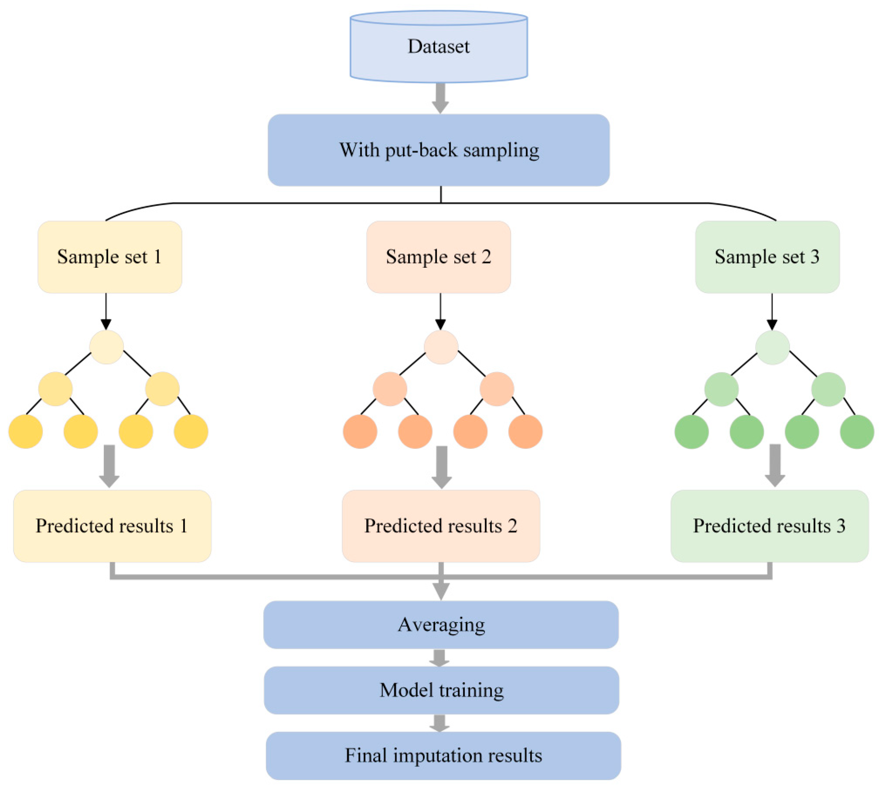
Random forest was proposed by Leo [24] in 2001. It is an ensemble learning method that improves the overall model performance and accuracy by constructing multiple decision trees and combining their prediction results. During training, each tree is built using a randomly selected subset of samples from the original dataset, a process known as “bootstrap aggregating” or “bagging”. Throughout the construction of each tree, for each node’s split, a subset of features is randomly chosen to search for the optimal splitting point. Suppose we have a dataset containing samples and features. Random forest constructs decision trees, and the building process for each tree is as follows, with the decision-making process illustrated in Figure 1:
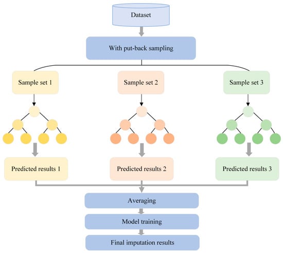
Figure 1.
Decision process in random forest.
Step 1. Sample Collection: Randomly draw samples with replacement from the dataset to form a training set .
Step 2. Feature Sampling: At each node split, randomly select features (where ). For each sample, after entering the decision tree, among the features at each decision node, identify the feature that best matches the data for branch splitting and repeat the decision process at the next node until the decision tree can no longer branch [25].
Step 3. Tree Construction: Use and the selected features to recursively split and build the decision tree until the stopping criteria are met.
Step 4. Missing Data Prediction: For a new sample , each tree provides a prediction . The final prediction for regression problems in random forest is the average of all tree predictions.
In the random forest model, the construction of each CART decision tree and the assessment of feature importance primarily rely on the following three key metrics: First, the Gini coefficient is an important measure of importance in random forest [26,27]; it is used to assess the impurity of nodes within the decision tree. Here, represents the proportion of samples belonging to class at node . The smaller the Gini coefficient, the higher the purity of the node, meaning the distribution of classes among the samples at the node is more uniform.
At the same time, the effectiveness of a split is evaluated by minimizing the squared differences between the data points within a node and the mean of the node. Here, is the number of samples at node , is the target value of the -th sample at node , and is the mean value of node .
The following formula evaluates the effectiveness of the splitting when a specific attribute value, , is selected as the splitting point in the decision tree. The optimal splitting point in a regression tree is identified by comparing the least squares deviation between the left and right child nodes post-split. This method enhances the tree’s prediction accuracy by ensuring that each split minimizes node variance, thus improving the tree’s overall data imputation precision.
2.2. SW-KNN Imputation
KNN selects the k-nearest neighbors based on the smallest distance to impute missing values, and it is popular due to its ease of implementation and good performance [28]. However, it performs poorly when the dataset is large or when the correlation between features is weak. Following the ideas presented in [29], we enhance this approach by assigning weights to each nearest neighbor based on the Spearman rank correlation coefficient instead of traditional Euclidean distance or other distance metrics. This modification helps capture the intrinsic patterns of other relevant features introduced, thereby improving the accuracy of imputation for missing power load values.
Step 1. Calculate the Spearman correlation coefficient using the formula consistent with the correlation analysis in Section 4.2. In the formula below, let , , and represent the original data, coefficient values, and total correlation coefficient of the -th feature with the -th feature, respectively. and indicate the influence weight and effective correlation coefficient of sample on missing value , and they are used in the calculation of only when sample is non-empty.
Step 2. Calculate the weights of distances between samples.
Step 3. Calculate the weighted distances between samples. Use as the weight to compute the Euclidean distance, then adjust the distances between samples using to balance the impact of varying amounts of missing values in each sample.
Step 4. Estimate missing values by weighting the values of the nearest samples with the effective coefficient .
2.3. LM-BP Imputation
BP neural networks are known for their excellent nonlinear characteristics, flexible and effective learning methods, and strong resistance to interference. They effectively account for the stochastic, nonlinear, and conditional features of power load, gaining widespread application in the practical estimation of missing values. However, the traditional BP algorithm based on standard gradient descent often struggles with convergence issues, affecting the quality of the solutions in practical problems. Since the Levenberg–Marquardt method (hereafter referred to as LM) offers the fastest convergence speed and higher computational accuracy for small- to medium-sized neural networks, we consider using LM-BP to impute missing power load values. The training process is as follows:
Step 1. Determine the neural network structure and initialize weights and thresholds: The optimal network structure and learning rate will be discussed in Section 4.1. Initialize the weights and thresholds from the input layer to the hidden layer and from the hidden layer to the output layer with random values in the range of .
Step 2. Carry out a forward propagation calculation: Conduct forward propagation through the determined network structure, calculating the output of the hidden layer and the output layer . is the weight from the input layer to the hidden layer, is the threshold of the hidden layer, is the number of nodes in the hidden layer, is the weight from the hidden layer to the output layer, and is the threshold of the output layer.
Step 3. Determine the error calculation: Compute the prediction error , which is the difference between the expected value and the predicted value .
Step 4. Update the weights and thresholds: Update the weights and thresholds and in the network based on the calculated prediction error .
Step 5. Meet the iteration stopping condition: Continue updating the parameters iteratively until the mean square error is less than a predetermined threshold. Once this condition is met, terminate the iteration and conclude the training of the BP neural network.
The Levenberg–Marquardt algorithm is an optimization technique specifically designed to address nonlinear least squares problems. Its core strategy involves using the first derivatives (Jacobian matrix) and second derivatives (Hessian matrix) of network performance metrics for linear approximations. It seeks a small parameter change that reduces the error function , proving to be more robust and efficient in handling nonlinear issues [30]. In the algorithm, is referred to as the damping factor. fff represents a hypothetical function relationship, and is the Jacobian matrix of , containing the first derivatives of network performance metrics with respect to weights and thresholds. The specific calculation formula is as follows:
3. Variance–Covariance Hybrid Imputation Model
The randomness, nonlinearity, and conditionality of electric load can impede the accuracy improvement of a single model’s imputation. By introducing a variance–covariance weighting method, the combined approach integrates the random forest, SW-KNN, and LM-BP models and employs a dynamic distribution method of variance–covariance weights to merge the prediction results of these three algorithms. It dynamically allocates weights , , and based on the variance and covariance of the imputation results from each model: , , and . This method quantifies each model’s prediction error and correlation, thereby synthesizing each model’s prediction results more accurately. In the formula, represents the variance of the imputed samples. The overall model structure is illustrated in Figure 2.
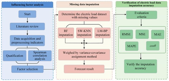
Figure 2.
Proposed model structure.
4. An Example Analysis Based on the Hybrid Model
4.1. Data Source and Processing
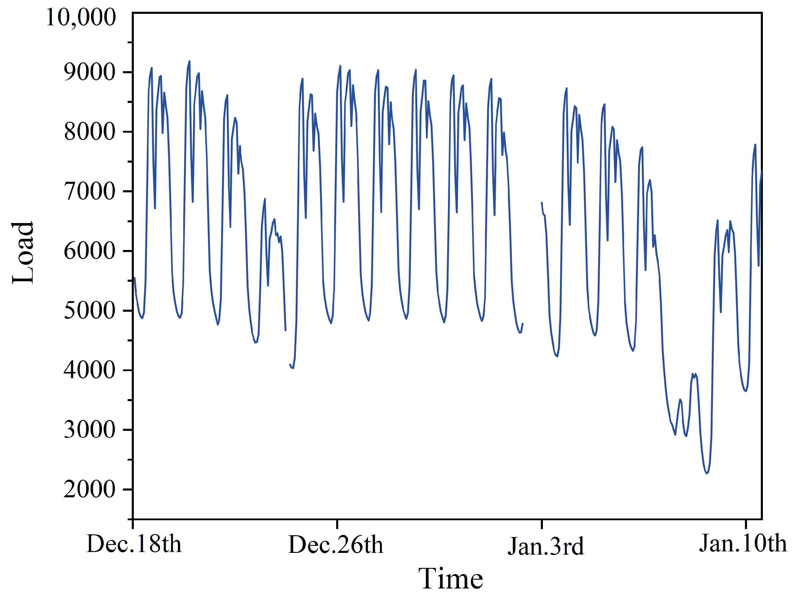
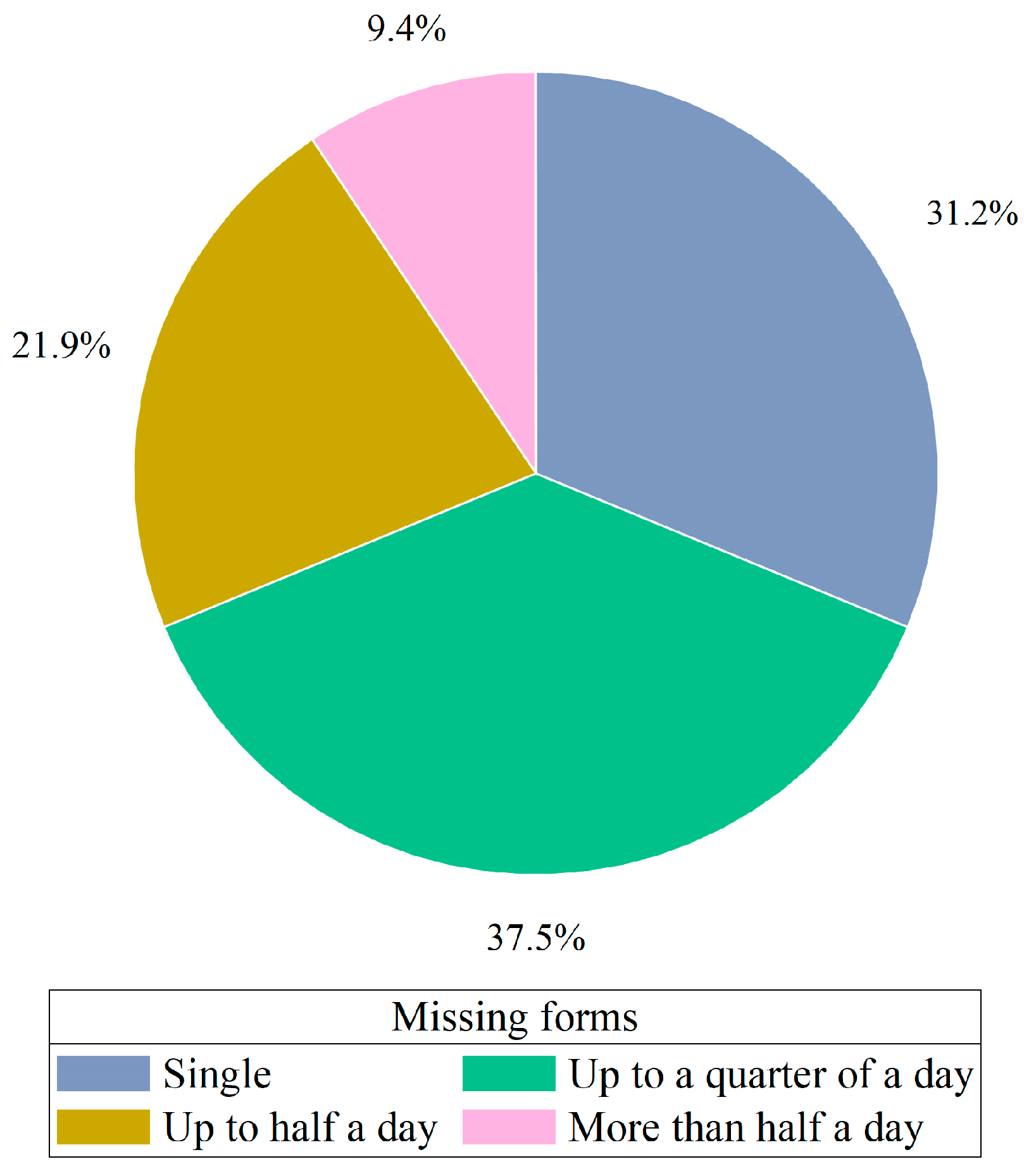
To verify the effectiveness of the variance–covariance weighted combination machine learning model, this study utilizes electric load data from a location in Southern China. The data spans from 1 January 2014 to 9 January 2015, with the dataset sampled every 60 min, providing 24 data points per day and a total of 8952 data points. The example of missing original data is illustrated in Figure 3. Among these, 128 values are missing, corresponding to a missing rate of 1.430%. The missing values occur in various forms: as single instances, lasting up to a quarter of a day, up to half a day, and for more than half a day. The lengths of these missing intervals are 1, (1, 6], (6, 12], and (12, ∞), respectively. The distribution of these missing values is illustrated in the pie chart shown in Figure 4. Unless otherwise noted, we selected data from the first seven days as the training set and selected data from the remaining day, which contain missing values, as the testing set to assess the performance of the imputation. More detailed selections will be discussed in Section 4.4.4. The experiments were conducted using Pycharm IDE (PC-232.10072.31) and the TensorFlow 2.6.0 framework. The hardware used included an AMD Ryzen 7 5800H processor, manufactured by Advanced Micro Devices, Inc. (AMD) in Santa Clara, California, USA, and an NVIDIA GeForce RTX 3060 GPU, produced by NVIDIA Corporation in Santa Clara, California, USA, with 16 GB of memory, supplied by a manufacturer based in Dongguan, China. The parameters for each model were set as shown in Table 1.
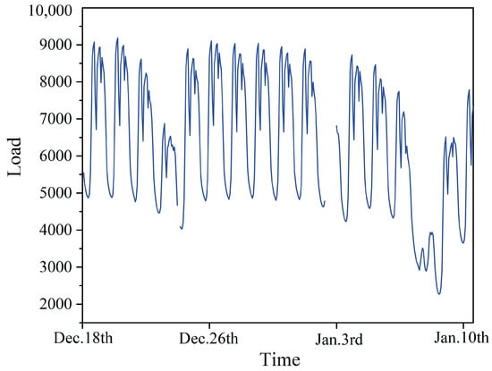
Figure 3.
Example of missing original data from 2014.
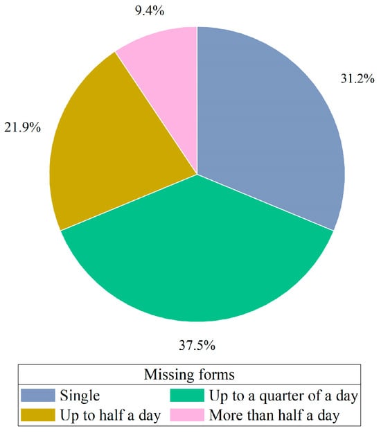
Figure 4.
Pie chart of missing form distribution.

Table 1.
Parameter optimization for each algorithm.
4.2. Feature Selection
The purpose of a correlation analysis is to examine the degree of association between two variables to reduce data redundancy. Given that not all indicators follow a normal distribution, we used the Spearman rank correlation coefficient to assess the relationships between metrics. The Spearman rank correlation coefficient is defined as the Pearson correlation coefficient calculated for ranked variables. When the sample size is , the original dataset with observations is transformed into ranked data, and the correlation coefficient is represented. In cases where data do not share the same rank, a simplified formula may be used to express the Spearman coefficient:
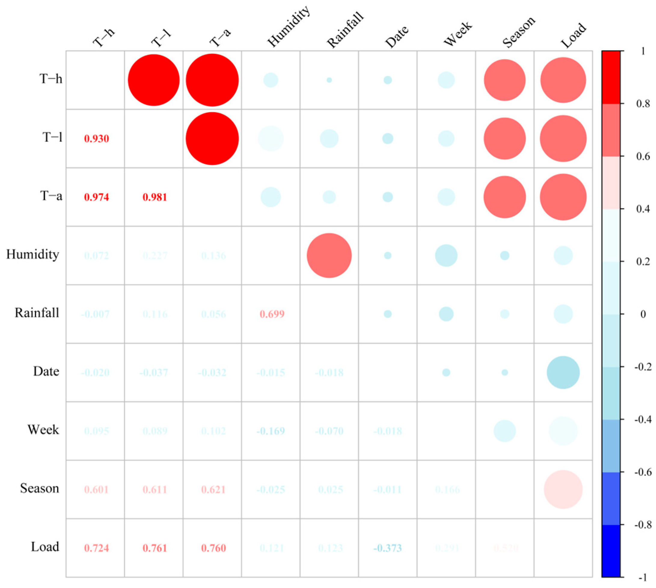
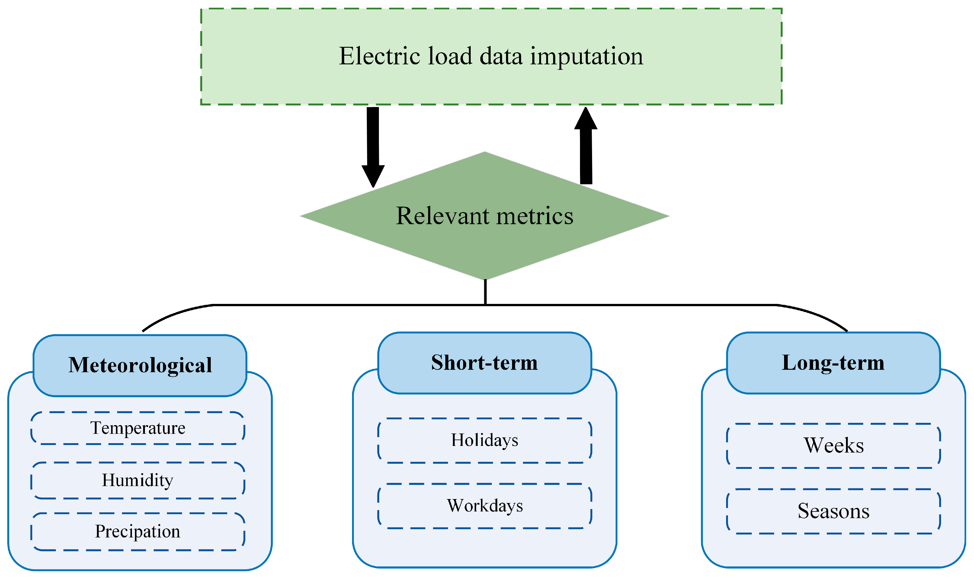
A correlation analysis of input characteristics is shown in Figure 5. Here, “humidity” represents the relative humidity, and “rainfall” represents the amount of rainfall in a day. Specifically, we quantified “date” into categories of holidays and workdays, as detailed in Table 2. The terms “week” and “season”, respectively, represent the ordinal numbers of the week and season. , , and represent the highest, lowest, and average temperatures of the day, while “load” represents the average daily electric load. In the correlation heatmap, we observed that temperature has the strongest correlation with electric load, exceeding 0.7, while relative humidity, rainfall, and week show weaker correlations with electric load at 0.12, 0.12, and 0.29, respectively. We believe that factors with a correlation coefficient greater than 0.3 can be selected as input features for model training [31]. Therefore, temperature, date type, and season, among a total of five factors, were finally chosen to assist in model training and missing value imputation.. The input correlation factors of electric load is illustrated in Figure 6.

Figure 5.
Heatmap for correlation analysis.
Table 2.
Quantification of date factors.
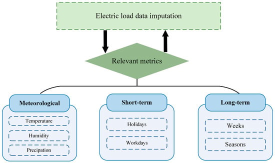
Figure 6.
Input correlation factors of electric load.
4.3. Evaluation Metrics
To demonstrate the imputation accuracy of the variance–covariance weighted hybrid imputation model, we compared multiple imputation methods using the root mean square error (RMSE), mean absolute error (MAE), mean absolute percentage error (MAPE), and cosine similarity () as evaluation criteria. The RMSE encapsulates the statistical properties of the differences, the MSE effectively reflects the accuracy of model predictions, the MAE represents the average of the absolute values of the prediction errors, and the MAPE indicates the average magnitude of the absolute differences. Lower values of the RMSE, MSE, MAE, and MAPE indicate better model performance. Additionally, we used cosine similarity to measure the similarity in trends between the imputed data and the original data. A cosine similarity close to 1 during fitting suggests that the two sequences are nearly identical. If the similarity is significantly less than 1, even if other error metrics perform well, it may indicate that, despite there being small errors between predicted and actual values, their trends may not align. Let be the predicted value; the true value in the sample; and the number of imputations. The specific formulas are as follows:
4.4. Experimental Results and Analysis
4.4.1. Comparison between Single Model and Multiple Models
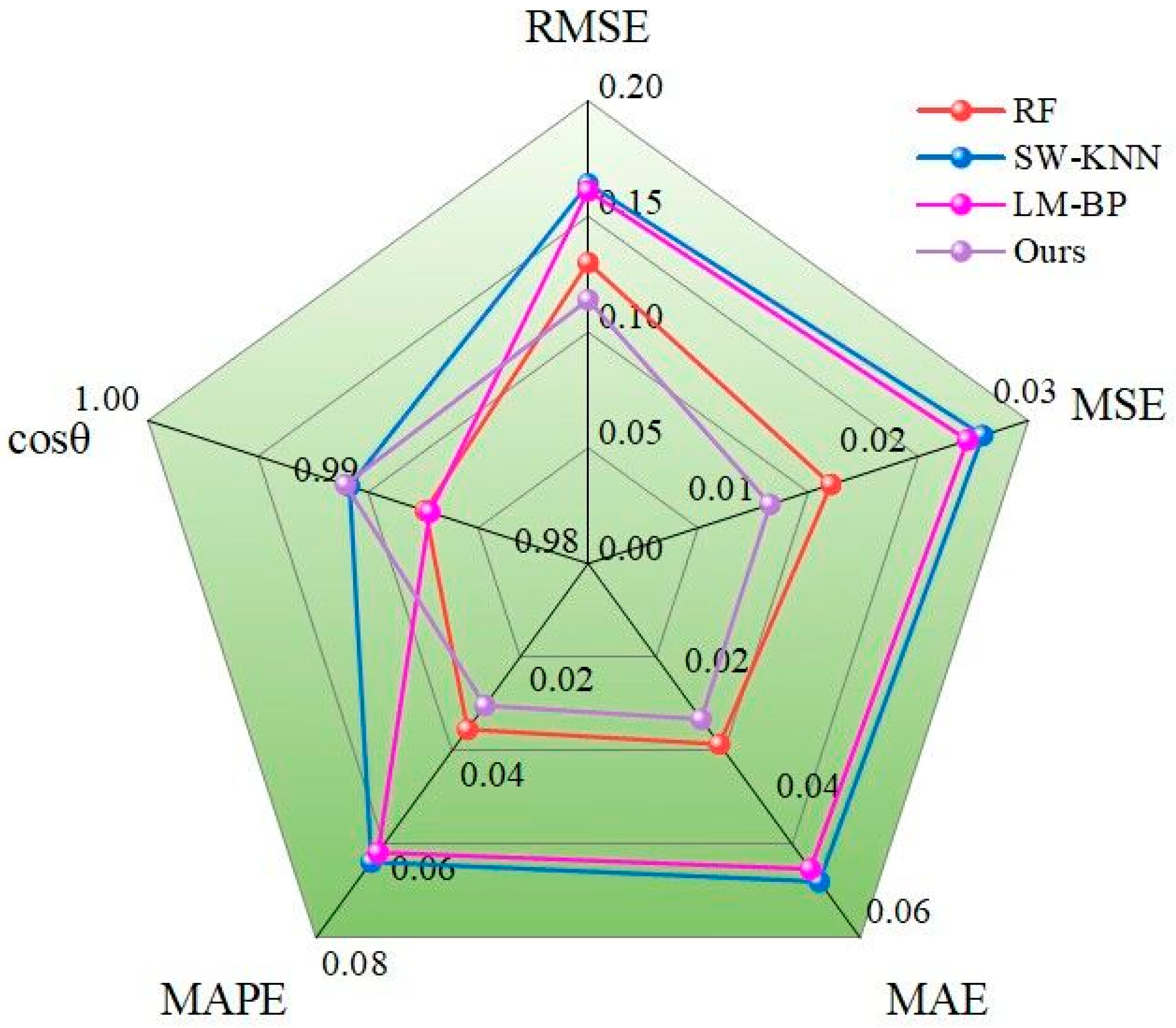
We input the original dataset, which includes missing values, into the model, applying three different imputation techniques: RF, SW-KNN, and LM-BP. After filling the missing values, the predictions were combined using the variance–covariance weighted model to produce our final results. We demonstrated the superiority of our model’s imputation by comparing the predictive results of the individual and combined models with the actual outcomes.
As shown in Figure 7, the improved hybrid model effectively combines the strengths of the three methods, taking into account the uncertainty of missing data. The improvements in the RMSE, MSE, MAE, and MAPE compared to the previously best model are 12.3%, 23.5%, 13.8%, 17.1%, and 0.02%, respectively, indicating higher prediction accuracy.
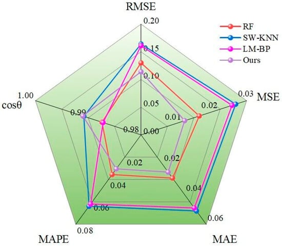
Figure 7.
Radar chart comparing hybrid model with individual models.
4.4.2. Comparison of Different Variants
We compared the current model with other combined models, including simple averaging, stacking methods, and the optimal weighted combination model. In the simple averaging approach, the final imputation result was derived by averaging three methods: RF, SW-KNN, and LM-BP. In the stacking method, base learners were trained using the three algorithms on the training set, and their outputs were combined to form a new training set to train the meta-learner and assign weights. After evaluating multiple meta-learners, Extra Trees (ET) was selected as the meta-learner for this study due to its relatively good generalization ability and excellent performance. Finally, the model was evaluated using the testing set. This structured approach ensured that the comparisons and methodologies are clearly understood and formally presented.
As indicated in Table 3, employing the variance–covariance variable weight combination method enhanced the performance of all three models. In contrast, simply averaging the results overlooked performance differences and correlations among the models under various conditions, thereby preventing the full leverage of each model’s strengths. This occurred because contributions from all models were averaged out, and poorly performing models can negatively impact the overall predictive performance. Although the stacking method improves the performance relative to simple averaging, its efficacy heavily depends on the choice of the meta-model. Due to the potential for overfitting in the meta-model, its generalization capability on the testing set may be compromised, rendering its performance inferior to the variance–covariance variable weight combination method. This structured analysis clarifies the advantages and limitations of each method in the context of model integration strategies.
Table 3.
Comparison of ensemble methods for imputation accuracy.
Additionally, we compared the single and hybrid SW-KNN models with single and hybrid models of various other variants. The single model involves using a single KNN variant for imputing missing values, whereas the hybrid model employs a combined approach utilizing the variance–covariance method with RF and LM-BP. The results shown in Table 4 indicate that the hybrid model outperformed the single model in performance. Furthermore, SW-KNN demonstrated enhanced effectiveness over KNN, NAA [32], and WKNN [33]. This improvement arose because KNN naively performs imputation without accounting for the correlations between features. In contrast, SW-KNN accounts for the complex relationships among features when computing the weighted distance, ensuring data points with similar dimensions receive higher weights. This methodology enables a more accurate imputation of missing power load values, illustrating the advantages of integrating sophisticated data handling techniques.
Table 4.
Performance metrics of imputation methods across single and hybrid models.
4.4.3. Comparison with Other Methods
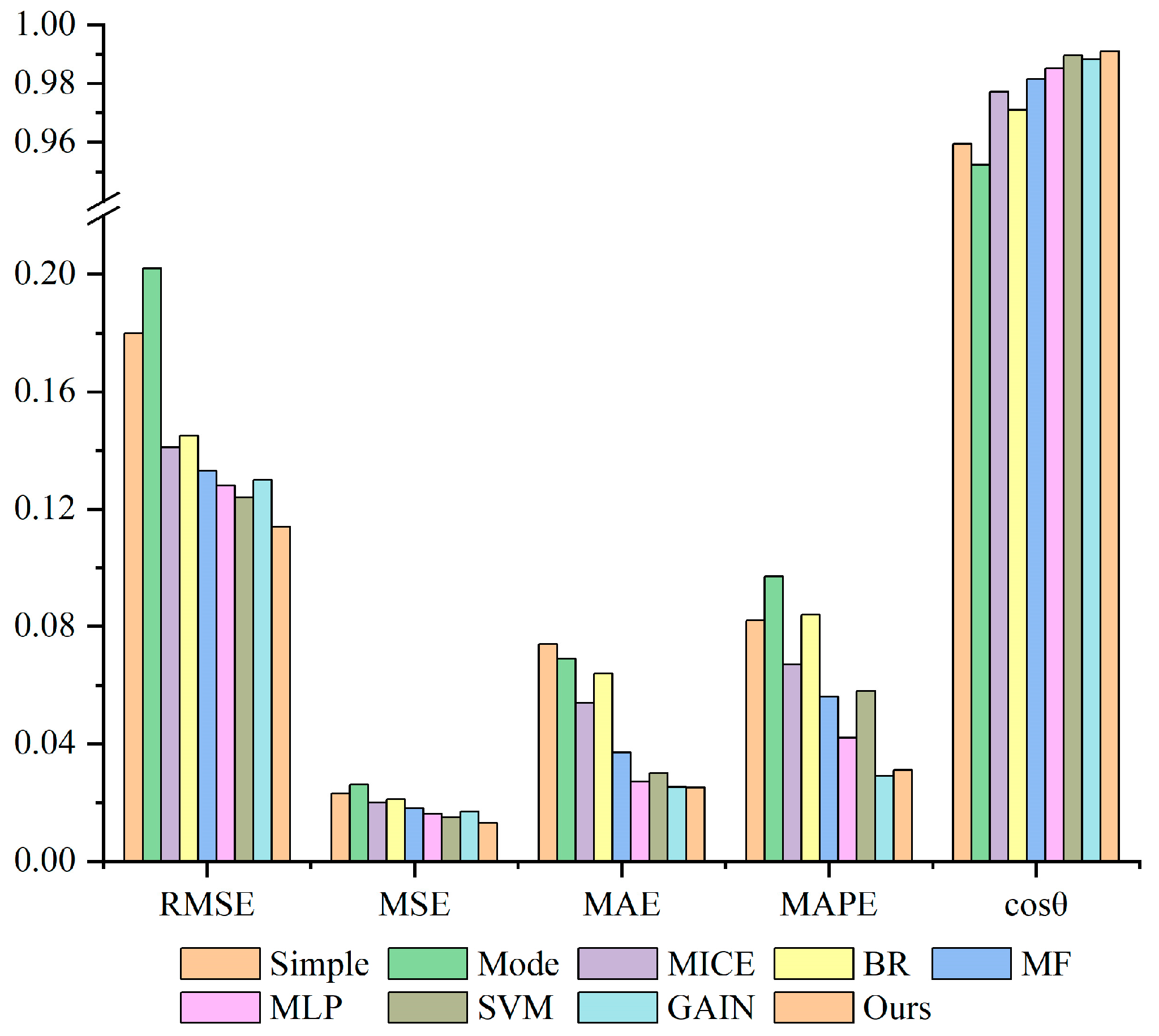
Figure 8 presents the results of the imputation experiments. Initially, it is observed that in all scenarios, the machine learning methods surpassed the traditional statistical methods, including the simple mean, mode, MICE, and Bayesian Regression. The performance differences range from 0.005 to 0.066 for RMSE; from 0.028 to 0.051 for MAPE; and from 0.0042 to 0.0316 for MAE. It is also noted that the advanced machine learning hybrid models consistently exhibited superior performance compared to other machine and deep learning models, such as MF and GAIN, in terms of the RMSE, MSE, and MAE, although their performance was comparable to that of GAIN in terms of the MAE and MAPE. Overall, the variance–covariance variable weight model achieved the highest performance. This structured approach ensures that the comparisons and outcomes are clearly understood and effectively communicated.
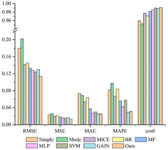
Figure 8.
Comparison with other methods.
4.4.4. Investigating the Impact of the Training Scale and Season
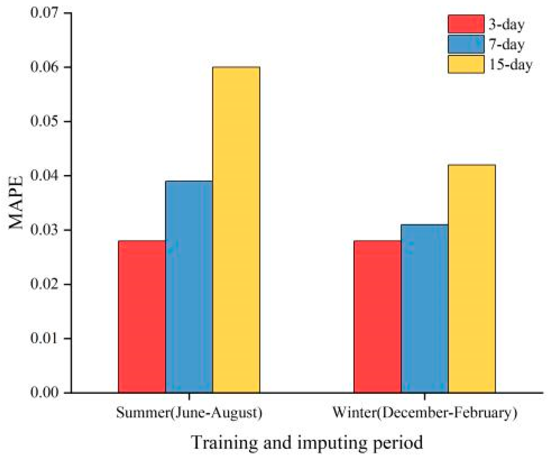
On one hand, we explored the impact of different seasons on imputation performance by changing the sampling dataset between summer and winter. On the other hand, we strictly controlled the number of imputations (10 missing data points in 1 day) and vary the size of the training set between 3 days, 7 days, and 15 days to measure the MAPE and RMSE under different conditions. Figure 9 and Figure 10 presents the results of different training periods in two seasons. Through controlled experiments, we found that winter generally yields better prediction results than summer, and shorter training periods tend to perform better than longer ones. This may be due to significant differences in weather conditions and user behavior patterns across seasons. In winter, the increased demand for heating due to lower temperatures leads to higher electricity loads, allowing the model to better capture load variations during this season. Furthermore, electric load forecasting exhibits strong daily periodicity, and larger training datasets may not facilitate capturing short-term dependencies in the time series effectively. The errors under different imputation conditions are shown in Table 5.
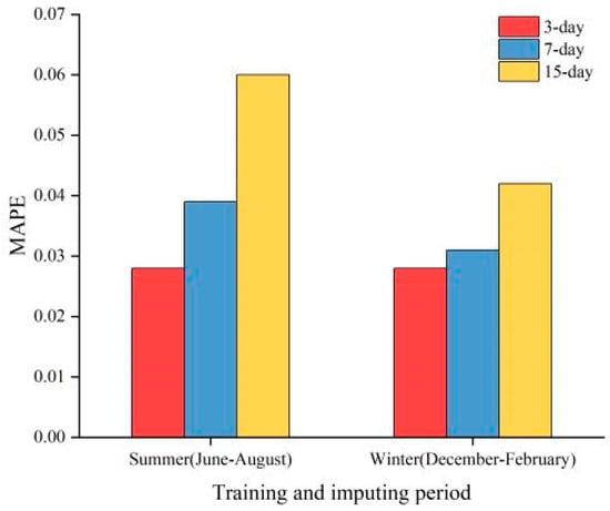
Figure 9.
MAPE for different training periods in two seasons.
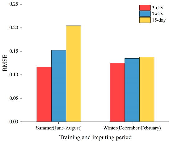
Figure 10.
RMSE for different training days in two seasons.
Table 5.
Errors under different imputation conditions.
4.4.5. Impact of Related Metrics on Imputation
The evaluation metrics for the hybrid imputation model under different features are shown in Table 6, where the “Feature” column indicates additional features added on top of the basic ones. The impacts of , , and on the model’s evaluation metrics are similar. Including all indicators, the model achieves an RMSE of 0.114, an MSE of 0.013, and an MAE of 0.022, indicating reductions ranging from 8.3% to 38.1%. The MAPE is 0.031, demonstrating a significant improvement, and the similarity of the score is 0.9910273, which is close to 1. This demonstrates that by incorporating meteorological and date factors, our model performs exceptionally well.
Table 6.
Impact of adding different factors on errors.
5. Conclusions and Outlook
In this study, we primarily assessed the performance of a hybrid model constructed from three machine learning methods designed for imputing consecutively missing feature values over extended periods, thereby enhancing the resilience and sustainability of smart grid operations. Additionally, we analyzed the performance differences across single and multiple models, various model variants, training set sizes, seasonal variations (summer and winter), and the inclusion of relevant factors for imputation, providing a comprehensive overview of how these variables impact model efficacy. Through tests on five distinct metrics, the hybrid model reduced the RMSE, MSE, MAE, and MAPE by approximately 12.3–23.5% compared to the best single model. Considering different factors, the reductions in RMSE, MSE, and MAE ranged from 8.3 to 38.1%, with improvements in slightly increasing and trending towards 1. Moreover, the machine learning hybrid model demonstrated superior imputation accuracy compared to different variants and mainstream imputation methods. This demonstrates the precision and superiority of considering multiple factors and applying the variance–covariance weighted method, highlighting the significant potential of our model in enhancing data accuracy and ensuring reliable energy management.
Looking ahead, future research should focus on refining this hybrid approach to better align with the goals of sustainable development and energy security. Our method comprehensively considers both meteorological features and the short-term and long-term factors of time series to enhance the accuracy and efficiency of data imputation. This study detailed the application of three machine learning models—random forest (RF), k-nearest neighbors based on Spearman’s rank correlation coefficient (SW-KNN), and back propagation neural network optimized by the Levenberg–Marquardt (LM-BP) method. Moreover, we introduced a variance–covariance weighted mixing imputation model that combines the predictive results of these models, dynamically allocating weights based on their variance and covariance to synthesize more accurate outcomes. These advancements support the transition to a green energy future by providing actionable insights and reliable data for optimizing power grid operations. By integrating these advanced techniques, this study offers a clear pathway to practical applications that enhance operational efficiency and promote environmental sustainability. Additionally, real-time data integration and dynamic prediction updates will be critical for maintaining grid stability and efficiency, ensuring that smart grids continue to meet the evolving demands of a sustainable energy landscape. This study lays a strong foundation for future advancements in sustainable energy management within intelligent power systems, offering a comprehensive approach that addresses complex dependencies among features and improves the stability and accuracy of power grid operations.
Author Contributions
Conceptualization, Z.H. and J.L.; methodology, Z.H.; software, J.L.; validation, Z.H. and J.L.; formal analysis, J.L.; investigation, Z.H.; resources, Z.H.; data curation, J.L.; writing—original draft preparation, Z.H.; writing—review and editing, Z.H.; visualization, J.L.; supervision, Z.H.; project administration, Z.H. and J.L.; funding acquisition, Z.H. All authors have read and agreed to the published version of the manuscript.
Funding
This research received no external funding.
Institutional Review Board Statement
Not applicable.
Data Availability Statement
The data presented in this study are available upon request from the corresponding author.
Conflicts of Interest
The authors declare no conflicts of interest.
References
- Liu, X.; Zhang, Z. A Two-Stage Deep Autoencoder-Based Missing Data Imputation Method for Wind Farm SCADA Data. IEEE Sens. J. 2021, 21, 10933–10945. [Google Scholar] [CrossRef]
- Humeau, S.; Wijaya, T.K.; Vasirani, M.; Aberer, K. Electricity load forecasting for residential customers: Exploiting aggregation and correlation between households. In Proceedings of the 2013 IEEE Sustainable Internet and ICT for Sustainability (SustainIT), Palermo, Italy, 30–31 October 2013; pp. 1–6. [Google Scholar]
- Sharma, S.; Verma, V. Performance of Shunt Active Power Filter Under Sensor Failure. In Proceedings of the 2017 IEEE International WIE Conference on Electrical and Computer Engineering (WIECON-ECE), Dehradun, India, 18–19 December 2017; pp. 165–168. [Google Scholar]
- Zhou, X.; Han, X.; Wu, Y.; Ju, R.; Tang, Y.; Ni, M. Vulnerability Assessment of the Electric Power and Communication Composite System. In Proceedings of the 2014 IEEE China International Conference on Electricity Distribution (CICED), Shenzhen, China, 23–26 September 2014; pp. 369–372. [Google Scholar]
- Dai, Y.; Chen, Z.; Zheng, X.; Dong, X.; Du, Y.; Liu, X. Smart Electricity Meter Reliability Analysis Based on In-Service Data. In Proceedings of the 2021 IEEE 4th International Conference on Energy, Electrical and Power Engineering (CEEPE), Chongqing, China, 23–25 April 2021; pp. 143–147. [Google Scholar]
- Das, P.; Shuvro, R.A.; Wang, Z.; Hayat, M.M.; Sorrentino, F. A Data-Driven Model for Simulating the Evolution of Transmission Line Failure in Power Grids. In Proceedings of the 2018 IEEE North American Power Symposium (NAPS), Fargo, ND, USA, 9–11 September 2018; pp. 1–6. [Google Scholar]
- Kong, W.; Dong, Z.Y.; Jia, Y.; Hill, D.J.; Xu, Y.; Zhang, Y. Short-Term Residential Load Forecasting Based on LSTM Recurrent Neural Network. IEEE Trans. Smart Grid 2019, 10, 841–851. [Google Scholar] [CrossRef]
- Sim, Y.-S.; Hwang, J.-S.; Mun, S.-D.; Kim, T.-J.; Chang, S.J. Missing Data Imputation Algorithm for Transmission Systems Based on Multivariate Imputation with Principal Component Analysis. IEEE Access 2022, 10, 83195–83203. [Google Scholar] [CrossRef]
- Miranda, V.; Krstulovic, J.; Keko, H.; Moreira, C.; Pereira, J. Reconstructing Missing Data in State Estimation with Autoencoders. IEEE Trans. Power Syst. 2012, 27, 604–611. [Google Scholar] [CrossRef]
- Konstantinopoulos, S.; De Mijolla, G.M.; Chow, J.H.; Lev-Ari, H.; Wang, M. Synchrophasor Missing Data Recovery via Data-Driven Filtering. IEEE Trans. Smart Grid 2020, 11, 4321–4330. [Google Scholar] [CrossRef]
- Sun, J.; Liao, H.; Upadhyaya, B.R. A Robust Functional-Data-Analysis Method for Data Recovery in Multichannel Sensor Systems. IEEE Trans. Cybern. 2014, 44, 1420–1431. [Google Scholar] [CrossRef] [PubMed]
- Suo, Q.; Zhong, W.; Xun, G.; Sun, J.; Chen, C.; Zhang, A. GLIMA: Global and Local Time Series Imputation with Multi-Directional Attention Learning. In Proceedings of the 2020 IEEE International Conference on Big Data (Big Data), Atlanta, GA, USA, 10–13 December 2020; pp. 798–807. [Google Scholar]
- Lin, W.-C.; Tsai, C.-F. Missing Value Imputation: A Review and Analysis of the Literature (2006–2017). Artif. Intell. Rev. 2020, 53, 1487–1509. [Google Scholar] [CrossRef]
- Azarkhail, M.; Woytowitz, P. Uncertainty Management in Model-Based Imputation for Missing Data. In Proceedings of the 2013 IEEE Proceedings Annual Reliability and Maintainability Symposium (RAMS), Orlando, FL, USA, 28–31 January 2013; pp. 1–7. [Google Scholar]
- Kamisan, N.A.B.; Lee, M.H.; Hussin, A.G.; Zubairi, Y.Z. Imputation Techniques for Incomplete Load Data Based on Seasonality and Orientation of the Missing Values. Sains Malays. 2020, 49, 1165–1174. [Google Scholar] [CrossRef]
- Farrugia, M.; Scerri, K.; Sammut, A. Imputation of Electrical Load Profile Data as Derived from Smart Meters. In Proceedings of the 2022 IEEE 21st Mediterranean Electrotechnical Conference (MELECON), Palermo, Italy, 14–16 June 2022; pp. 1067–1072. [Google Scholar]
- Crespo Turrado, C.; Sánchez Lasheras, F.; Calvo-Rollé, J.; Piñón-Pazos, A.; De Cos Juez, F. A New Missing Data Imputation Algorithm Applied to Electrical Data Loggers. Sensors 2015, 15, 31069–31082. [Google Scholar] [CrossRef] [PubMed]
- Smola, A.J.; Vishwanathan, S.V.; Hofmann, T. Kernel methods for missing variables. In Proceedings of the International Conference on Artificial Intelligence and Statistics, Las Vegas, NV, USA, 27–30 June 2005; pp. 325–332. [Google Scholar]
- Huo, H.; Xu, D.; Ding, L.; Liu, Y.; Zheng, Y.; Wang, S.; Xin, C.; Li, W. A Comprehensive Analysis Framework for Power Grid Construction and Operation Efficiency Consider Regional Differentiation and Load Randomness. In Proceedings of the 2023 IEEE 3rd International Conference on Energy Engineering and Power Systems (EEPS), Dali, China, 28 July 2023; pp. 891–896. [Google Scholar]
- Ahmadi, M.M.H.; Aghasi, S.H.; Salemnia, A. Hybrid Energy Storage for DC Microgrid Performance Improvement Under Nonlinear and Pulsed Load Conditions. In Proceedings of the 2018 IEEE Smart Grid Conference (SGC), Sanandaj, Iran, 28–30 November 2018; pp. 1–6. [Google Scholar]
- Lotfipoor, A.; Patidar, S.; Jenkins, D.P. Transformer Network for Data Imputation in Electricity Demand Data. Energy Build. 2023, 300, 113675. [Google Scholar] [CrossRef]
- Ryu, S.; Kim, M.; Kim, H. Denoising Autoencoder-Based Missing Value Imputation for Smart Meters. IEEE Access 2020, 8, 40656–40666. [Google Scholar] [CrossRef]
- Liu, Z.; Tao, Y.; Liu, H.; Luo, L.; Zhang, D.; Meng, X. Missing Completion Method for Load Data Based on Generative Adversarial Imputation Net. In Proceedings of the 2023 IEEE International Conference on Power Science and Technology (ICPST), Kunming, China, 5–7 May 2023; pp. 294–298. [Google Scholar]
- Breiman, L. Random Forests. Mach. Learn. 2001, 45, 5–32. [Google Scholar] [CrossRef]
- Ou, H.; Yao, Y.; He, Y. Missing Data Imputation Method Combining Random Forest and Generative Adversarial Imputation Network. Sensors 2024, 24, 1112. [Google Scholar] [CrossRef] [PubMed]
- Wang, M.; Ye, X.-W.; Ying, X.-H.; Jia, J.-D.; Ding, Y.; Zhang, D.; Sun, F. Data Imputation of Soil Pressure on Shield Tunnel Lining Based on Random Forest Model. Sensors 2024, 24, 1560. [Google Scholar] [CrossRef] [PubMed]
- Algehyne, E.A.; Jibril, M.L.; Algehainy, N.A.; Alamri, O.A.; Alzahrani, A.K. Fuzzy Neural Network Expert System with an Improved Gini Index Random Forest-Based Feature Importance Measure Algorithm for Early Diagnosis of Breast Cancer in Saudi Arabia. Big Data Cogn. Comput. 2022, 6, 13. [Google Scholar] [CrossRef]
- Yang, F.; Du, J.; Lang, J.; Lu, W.; Liu, L.; Jin, C.; Kang, Q. Missing Value Estimation Methods Research for Arrhythmia Classification Using the Modified Kernel Difference-Weighted KNN Algorithms. BioMed Res. Int. 2020, 2020, 7141725. [Google Scholar] [CrossRef] [PubMed]
- Liang, C.; Zhang, L.; Wan, Z.; Li, D.; Li, D.; Li, W. An Improved kNN Method Based on Spearman’s Rank Correlation for Handling Medical Missing Values. In Proceedings of the 2022 IEEE International Conference on Machine Learning and Knowledge Engineering (MLKE), Guilin, China, 25–27 February 2022; pp. 139–142. [Google Scholar]
- Ma, F.; Wang, S.; Xie, T.; Sun, C. Regional Logistics Express Demand Forecasting Based on Improved GA-BP Neural Network with Indicator Data Characteristics. Appl. Sci. 2024, 14, 6766. [Google Scholar] [CrossRef]
- Chen, H.; Zhu, M.; Hu, X.; Wang, J.; Sun, Y.; Yang, J. Research on Short-Term Load Forecasting of New-Type Power System Based on GCN-LSTM Considering Multiple Influencing Factors. Energy Rep. 2023, 9, 1022–1031. [Google Scholar] [CrossRef]
- Aidos, H.; Tomas, P. Neighborhood-Aware Autoencoder for Missing Value Imputation. In Proceedings of the 2020 IEEE 28th European Signal Processing Conference (EUSIPCO), Amsterdam, The Netherlands, 18–21 January 2021; pp. 1542–1546. [Google Scholar]
- Gond, V.K.; Dubey, A.; Rasool, A.; Khare, N. Missing Value Imputation Using Weighted KNN and Genetic Algorithm. In Proceedings of the ICT Analysis and Applications; Fong, S., Dey, N., Joshi, A., Eds.; Springer Nature: Singapore, 2023; pp. 161–169. [Google Scholar]


Disclaimer/Publisher’s Note: The statements, opinions and data contained in all publications are solely those of the individual author(s) and contributor(s) and not of MDPI and/or the editor(s). MDPI and/or the editor(s) disclaim responsibility for any injury to people or property resulting from any ideas, methods, instructions or products referred to in the content. |
© 2024 by the authors. Licensee MDPI, Basel, Switzerland. This article is an open access article distributed under the terms and conditions of the Creative Commons Attribution (CC BY) license (https://creativecommons.org/licenses/by/4.0/).