Abstract
This paper examined the practical impact of price-based demand-side management (DSM) for occupants of an office building connected to a renewable energy microgrid. There has been an absence of studies that have analyzed occupant reactions, in terms of perceived practicality, regarding the implementation of DSM in conjunction with factors including renewable energy generation, load shifting and energy costs. An increased understanding of the practicality of DSM will support future improvements in building energy efficiency and sustainability. Ten occupants of the National Build Energy Retrofit Test-bed (NBERT) were selected as a case study. The electricity consumption pattern of the NBERT occupants was derived over a period of two years. Five unique DSM schedules were developed for each of the NBERT occupants, and a survey was carried out to investigate the practicality of these DSM schedules. A real-time electricity pricing tariff, electricity CO2 intensity, three feed-in tariffs and two microgrid control methods were evaluated to assess the practicality of each DSM schedule on the ten NBERT occupants. The results showed that the incorporation of onsite renewable energy generation with price-based DSM had a positive impact (r = 0.69–0.75) on occupant practicality. Onsite renewable energy generation was able to offset the demand for expensive electricity from the grid during peak hours, which aligned with the occupants’ typical work schedules. However, the introduction of a feed-in tariff with a renewable energy microgrid made price-based DSM less practical (r = 0.15–0.64).
1. Introduction
Demand-side management (DSM) is the planning and implementing of strategies designed to encourage consumers to improve their energy efficiency, reduce energy costs, change the time of energy usage and increase the utilization of renewable energy sources. It is a partnership between the energy utility and energy users that benefits both parties and is an important means of assisting the decarbonization of the energy sector.
The aim of DSM is to reduce peak loads and change the shape of load profiles through energy conservation techniques, peak clipping and load shifting. The correct implementation of DSM can be used to reduce energy consumption, maintain power quality and optimize the supply from renewable energy sources, resulting in financial and environmental benefits [1]. There are a number of methods for implementing DSM, including increasing energy efficiency, strategic load growth and demand response (DR). The implementation of DSM can require significant investment in infrastructure, such as monitoring sensors, although typically, the economic and financial benefits far outweigh the costs. Another drawback associated with DSM is the potential negative impacts that DSM strategies such as DR can have on user comfort and satisfaction, and the practicality of DSM is often overlooked [2].
Practicality with regard to DSM relates to the level of convenience for electricity consumers to partake in a particular DSM schedule [3]. The ability to quantify the practicality of potential DSM schedules may allow energy managers to tailor energy usage from the national grid and/or in a renewable energy microgrid (REµG) to optimize consumer comfort, increase energy efficiency, reduce energy demand, reduce monetary costs and/or lower carbon emissions. Electricity is more expensive at certain peak periods of the day when people use more electricity, such as when people wake up, arrive at their place of work and return home in the evening. Real-time pricing (RTP) is based on the national smart grid energy demand and fuel mix, which is heavily influenced by the daily schedules of the Irish population [4]. Current DSM research has focused on controlling electricity loads to minimize energy, monetary or CO2 costs by treating electricity loads as either interruptible and deferrable tasks (e.g., thermal storage), non-interruptible and deferrable tasks (e.g., cooking) or non-interruptible and non-deferrable tasks (e.g., lighting). Interruptible tasks may be stopped and restarted accordingly to reduce the demand as required, while deferrable tasks may be delayed by a defined period before commencing the task.
Several DSM scheduling algorithms have been developed with the aim of reducing peak load demand through shifting the loads of domestic appliances such as washing machines, dishwashers and immersion water heating to periods of low energy, monetary or CO2 costs. These algorithms primarily focused on efficiency and the associated energy, monetary and/or CO2 savings that could be achieved through DSM and DR. Therefore, the practical impacts of DSM on the consumer’s schedule were not a priority. A DSM schedule that results in minimum energy, monetary or CO2 costs may be unsuitable, inconvenient and/or impossible to implement due to numerous constraints on the consumer. Moreover, load shifting for industrial and commercial consumers can be more limited due to constraints on office working hours and a greater amount of non-interruptible and non-deferrable tasks [5].
Zang et al. [6] proposed a demand-side consumption optimization algorithm that utilized load shifting and load interruption techniques to model energy consumption for residential consumers. This was combined with a decision-making algorithm from a grid operator’s point of view to optimize energy consumption and demand-side comfort. Sun et al. [7] proposed an economic load response model, which incorporated the price elasticity of demand to optimize power system utilization and enhance operator planning. The proposed method incorporated shiftable loads and peak shaving to enable independent system operators to assess consumer behaviors in various microgrid electrical energy supply scenarios and evaluate the impact of load response programs on energy cost reduction. The study also introduced a particle swarm optimization algorithm to solve optimization problems. Xie et al. [8] proposed an optimal scheduling model for multi-regional energy systems that considered DR and shared energy storage. Their model used a multi-objective optimization technique to minimize the total operating cost of an energy system and maximize the net environmental impact. Roshan and Ganga [9] used machine learning algorithms to develop an intelligent and interactive DSM strategy for residential consumers. They categorized high-power consumers based on their daily load profiles per quarter of the day and clipped the peak loads of classified consumers to curtail their consumption within the baseline power of each quarter. Menos-Aikateriniadis et al. [10] evaluated particle swarm optimization methods used in residential DR applications for the scheduling and control of various energy systems, including electric vehicles, energy storage, heating/cooling devices, distributed generation and residential appliances. An energy management strategy for a renewable-based electro-thermal residential microgrid was proposed by Pascual et al. [11]. They used a combination of energy storage systems (heat and battery) and DSM to minimize power peaks and fluctuations. Their results indicated a reduction of overvoltage events in low-voltage grids, saturation alleviation in transmission lines and an improvement in grid quality and stability.
Electricity pricing structures such as RTP, time-of-use pricing, day and night pricing and flat rate pricing have been shown to influence the effectiveness of DSM strategies. Zhang et al. [12] studied the optimal scheduling of smart homes’ energy consumption through the use of mixed-integer linear programming. Distributed energy resource operation and electricity-consuming household tasks were scheduled based on RTP, the electricity task time window and forecasted renewable energy output to minimize 1-day forecasted energy consumption costs. A peak demand charge scheme was also adopted to reduce the peak demand from the grid. The results from this research indicated potential cost savings and reductions in peak electricity consumption through reduced energy consumption and better energy management. A novel RTP algorithm for a future smart grid was proposed by Samadi et al. [13], which incorporated a smart power infrastructure comprised of several power subscribers sharing a common energy source. Each power subscriber was equipped with an energy consumption controller unit as part of its smart meter. The smart meters were then connected to the power grid and a communication infrastructure, which allowed for two-way communication between the smart meters. The study modeled subscribers’ preferences and their energy consumption patterns using carefully selected utility functions based on concepts from microeconomics. They also used an algorithm that optimized the energy consumption levels for each subscriber to maximize the aggregate utility of all subscribers in the system in a fair and efficient fashion. The results from the study showed that the energy provider could encourage desirable consumption patterns among the subscribers using RTP interactions. Further results showed that distributed algorithms can potentially benefit both subscribers and energy providers.
Numerous DSM-related studies have incorporated occupant-related information. However, a limited number of studies have focused on occupant reactions to the practicality of price-based DSM and DR strategies. Missaoui et al. [14] proposed a global model-based anticipative building energy management system that compromised between user comfort and energy cost while also taking into account occupant expectations and physical constraints (e.g., energy prices and power limitations). The simulation results showed that their proposed design led to a monetary cost reduction of approximately EUR 1 per day (EUR 365 per year), which could be used to encourage occupants to participate in a residential electrical load-control program. However, financial incentives may not always encourage participation. Fell et al. [15] conducted a survey on consumer acceptance of a range of demand-side response tariffs in the UK and found that a direct load-control tariff, which enabled the providers to cycle their heating off and on, was most acceptable, as it gave the customers a greater sense of control over their comfort and spending and was easier to use. Wallin et al. [3] conducted research on understanding consumer willingness to participate in various DR activities in relation to economic incentives. The study reported reduced participation in a DSM program involving an energy intervention framework that encouraged consumers to alter their consumption behavior during peak hours in December. Joe-Wong et al. [16] probabilistically modeled consumer willingness to shift their device usage based on parameters that can be estimated from real data. The study hypothesized that by charging users more for electricity in peak periods and less in off-peak periods, the electricity provider can induce users to shift their consumption to off-peak periods. Therefore, relieving stress on the power grid and reducing the cost incurred from large peak loads. Gao et al. [17] used a value function based on prospect theory to represent the risk attitude of consumers. The risk attitude of consumers was defined as the risk-taking attitude that organizations or individuals may have toward certain gains or losses that may arise through participating in DSM programs. Based on this function, the study proposed a variant Roth–Erev algorithm to characterize the uncertainty of consumer participation and measure the available capacity of DSM. They further generated DR schedules and constructed a DR scheduling model to reduce system operation costs. Concurrently, D’hulst et al. [18] used consumer comfort requirements to quantify DR flexibility for residential smart appliances. They proposed that flexibility potentials can be used as an instrument to determine the impact and economic viability of DR programs for residential premises.
It is clear from the literature that DSM may improve energy distribution efficiency, reduce energy costs, improve grid stability and increase the share of electricity generated by renewable sources [19]. However, it is questionable whether it is convenient for energy users to implement price-based DSM, and it is unclear if electricity users will accept DSM strategies. Thus, the practical impact on building occupant schedules must be considered when developing DSM strategies. None of the aforementioned studies have considered impacts on occupant schedules when developing DSM strategies. To the authors’ knowledge, no study has focused on quantifying how practical it would be to manipulate occupant schedules to generate energy savings. In addition, the introduction of renewable energy systems, such as solar photovoltaic (PV) and wind power systems, to a DSM strategy may have strong interactions with load-shifting patterns, energy costs, CO2 savings and consumer responses to DSM schedules. Venizelos et al. [20] recommended that considerable investigation is required to assess the potential cost risks and behavioral impacts for energy users in relation to price-based DSM integrated with PV systems. The introduction of renewable energy sources may result in conflicts between practicality for occupants and reducing energy, monetary or CO2 costs. Potential conflicts may depend on individual occupant preferences, electricity tariff structures, feed-in tariffs (FITs) and the type of renewable energy introduced.
This study utilized the occupants of the National Building Energy Retrofit Test-bed (NBERT) as a case study. The NBERT building is a smart building with an integrated REµG (PV and wind energy) and battery bank storage. A previous load-shifting study on the NBERT building by Phan et al. [21] focused on the daily charge and discharge schedule of a battery bank in order to minimize the operating cost of the building. Phan et al. [21] did not investigate modifying occupant schedules as a DSM technique nor did they investigate the practicality of applying DSM to an occupied office building. In this study, we focused on load shifting as a DSM technique and subsequently evaluated its practicality. This study had two primary objectives:
(1) Develop a price-based DSM practicality index to measure the level of inconvenience for the occupants of NBERT to partake in specific price-based DSM schedules;
(2) Evaluate the impacts that renewable energy, FITs and RTP have on the practicality of implementing price-based DSM using the REµG in NBERT as a case study.
The novelty and contribution of this body of work lies in the study of the occupants’ reactions to the practicality of price-based DSM. Numerous DSM-related studies have incorporated occupant-related information in their research, such as energy management schedules, electricity tariffs and willingness to participate in DSM activities. However, to the best of the authors’ knowledge, no study has focused on occupant reactions to the practicality of price-based DSM. An increased understanding of building occupant reactions to the practicality of DSM, in relation to REµGs, will support future developments in the areas of building energy efficiency and sustainability.
2. Materials and Methods
2.1. Electricity Consumption Data Collection
Electricity consumption profiles of the occupants (n = 10) of the NBERT, located in the Zero2020 building at the Munster Technological University (MTU), were derived as a case study for measuring the practicality of price-based DSM in an REµG. The NBERT building (https://messo.mtu.ie/nbert, accessed on 5 November 2023) is a smart building with an integrated REµG (PV and wind energy) and battery storage [21]. The REµG consisted of a 12 KWp PV system and a 12.6 KWp wind turbine. The PV system included 48 roof-mounted, south-facing polycrystalline panels, and more details relating to the REµG are presented in Phan et al.’s study [21].
The NBERT building contains state-of-the-art offices and meeting rooms for lecturers, researchers, industry consultants and visiting academics. The building is utilized as a testbed where occupants partake in a “living lab” environment for research focusing on human-dependent topics, including thermal comfort, DSM, renewable energy distribution and energy storage [21]. The NBERT office occupants consisted of four full-time lecturers (occupants A to D), four full-time administrative staff (occupants E to H) and two part-time administrative staff (occupants I and J). Each occupant of the NBERT office had a workstation, as shown in Figure 1 below. The workstation consisted of a PC/laptop, monitors and other electrical devices, such as printers, lights and speakers. The energy consumption of a workstation was monitored and recorded at 30 min intervals over a period of 24 months. There was a kitchenette in the office, which contained a water kettle and a coffee machine. The energy consumption of the kitchenette was recorded during tea/coffee making to determine the associated energy consumption. From these recordings, energy quantities (kWh) for each workstation and for making a cup of tea or coffee were empirically derived. These data were used to create the base work schedule (schedule 0) for each of the building occupants for five working days (Monday to Friday), using the following model:
where OEDi is the base occupant energy demand, WEDi is the energy demand for an occupant’s workstation, and TCEDi is the energy demand when an occupant decides to make tea or coffee, in kWh, for the ith 30 min interval of the occupants’ work schedule.
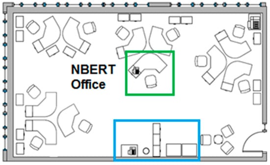
Figure 1.
Image illustrating the layout of the NBERT office; the blue box represents the kitchenette area, and the green box represents an occupant’s workstation.
An example of the base work schedule for occupant A is shown in Figure 2.

Figure 2.
Example of work schedule for occupant A. IO = the occupant was in the office with electrical devices switched on, IO* = the occupant was in the office and made a cup of tea using the kettle, L = the occupant left the office and went to the lecture hall, and the electrical devices at his or her workstation were on standby mode, and OF = the occupant was out of the office for a lunch break or personal reasons, and the electrical devices were on standby mode.
2.2. Demand Response Schedules
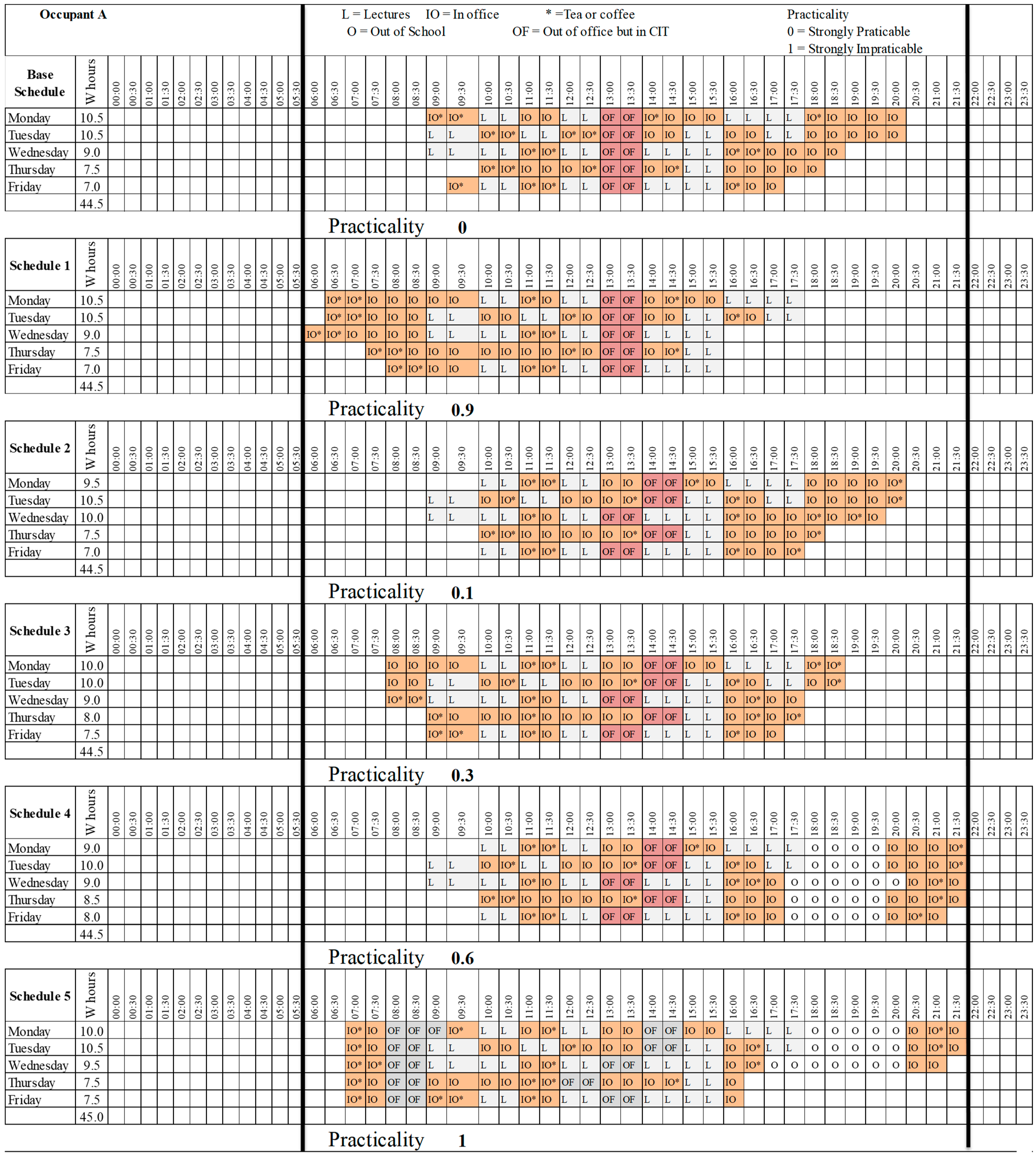
A customized base work schedule (schedule 0) was derived for each occupant of the NBERT office. This schedule was naturally the most practical schedule for the occupant, as it was dictated by their personal choices within the working time limits of 6 am to 10 pm, which were the office facility’s opening hours. Five additional work schedules (schedules 1–5) were generated for each of the NBERT office occupants. Each of the five schedules were unique for each occupant and simulated situations where the NBERT office occupants shifted their electricity usage to an off-peak period; thereby maximizing price-based DSM and theoretically reducing monetary, energy and CO2 costs and increasing the power supply from the onsite REµG. All the generated schedules for occupant A can be seen in Appendix A (Figure A1). To make the five generated DSM schedules and the base schedule comparable, the following five rules were imposed when generating the DSM schedules:
- The lecture times and durations were constant and could not be shifted.
- Work period boundaries of 6 am to 10 pm were set for all occupants.
- The total daily working hours for the five DSM schedules were equal to the total hours of each occupant’s base schedule.
- The total number of cups of tea and/or coffee consumed by each occupant was determined by their base schedule and kept constant for all new schedules.
- The total energy consumption was kept constant across all schedules for comparative purposes.
2.3. Structure of the Generated DSM Schedules
The generated DSM schedules followed the following structure for all occupants of the NBERT office:
- Schedule 1: The working hours of the occupants were shifted into early morning hours, thereby avoiding the critical peak period of electricity pricing (5 pm to 7 pm) for most of the occupants.
- Schedule 2: The working hours of the occupants were shifted into evening hours to compare working in critical peak periods in terms of practicality and energy cost reduction.
- Schedule 3: The base schedule was regenerated to create a balance between working in the early morning hours and working late in the evening; thus, schedule 3 represented a mid-point schedule between schedules 1 and 2.
- Schedule 4: This explored scenarios in which occupants came into the office early (6 am), left the office during the evening critical peak period (5 pm to 7 pm) and, afterwards, resumed work back in the office to complete their remaining work hours.
- Schedule 5: The occupants came into the office early (6 am) to take advantage of the low early morning electricity tariff. The occupants then left the office during the early morning peak period (8 am to 9 am). Afterwards, the occupants resumed work in the office and worked until the start of the evening critical peak period (5 pm). The occupants then left the office again during the evening critical peak period (5 pm to 7 pm) and resumed work in the office at 7 pm to complete their remaining work hours.
Schedule 4 and schedule 5 were developed to discern the willingness of the building occupants to observe unusual working hours to reduce electricity costs. Figure 3 displays the electricity demand of all 6 schedules along with the corresponding price and CO2 intensity of the electricity.
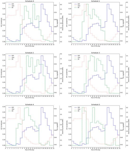
Figure 3.
Average electricity demand (ED) (kWh) of the NBERT office occupants versus real-time electricity price (RTP) (EUR/kWh) and CO2 emission factor (CO2) (kg/kWh) for the base (schedule 0) and five price-based DSM schedules. ED varies for each schedule.
2.4. Electricity Tariff, Feed-in Tariff and Renewable Energy Microgrid Configurations
The decision support tool for renewable energy microgrids (DSTREM) [21] was employed to simulate REµG electricity output, monetary income and associated CO2 emissions. The DSTREM is a tool that enables the users of buildings with an integrated REμG and smart grid connections to compare electricity tariffs, FITs, monetary income and associated CO2 emissions under different renewable energy system configurations through the use of control logic. Irish national grid data for the real-time pricing electricity tariff (RTPET), real-time electricity CO2 emissions (kg/kWh) and three stationary FIT structures for 2013 were used as inputs for the DSTREM under four different REµG configurations, namely no REµG, PV, wind and PV + wind. Real-time electricity CO2 emissions and demand on the national electricity grid data were provided by Eirgrid [22]. The RTPET represents a dynamic pricing structure based on the demand of the national smart grid, which varies depending on the hour of the day, day of the week and month of the year. The hourly average RTPET for the year 2013 was calculated and utilized. Figure 4 represents the hourly average dynamic RTP (EUR/kWh) and CO2 (kg/kWh) for 2013. The design of the RTPET is described in more detail in previous studies [4,21].
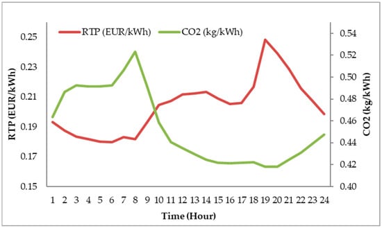
Figure 4.
Hourly averaged dynamic real-time pricing (RTP) (EUR/kWh) and CO2 emissions factor (kg/kWh) for the year 2013.
A FIT is the tariff payment made to households or businesses by public utility companies that generate renewable energy and sell excess output to the national smart grid. Before 2022, renewable energy FITs in Ireland ranged from 0 EUR/kWh to 0.19 EUR/kWh depending on the technology deployed [23,24]. To explore a wide range of FIT variation with respect to income and savings, three FITs were employed for this study, namely FIT0 (0 EUR/kWh), FIT9 (0.09 EUR/kWh) and FIT19 (0.19 EUR/kWh). This was based on a previous FIT structure where the first 3000 kWh of electricity exported to the national smart grid received 0.19 EUR/kWh and electricity exported after 3000 kWh received 0.09 EUR/kWh [25]. Electricity consumption (kWh), electricity costs (EUR/kWh) and avoided CO2 (kg/kWh) for all generated schedules in the REµG were simulated using DSTREM. Avoided CO2 refers to the quantity of CO2 emissions associated with electricity provided by the national grid that was displaced by electricity provided by the REµG.
2.5. Renewable Energy Microgrid Inputs, Control Methods and Simulations
Energy output for the REµG was simulated for the last seven days of the months of January, February, March, April, May, July and September for the year 2013. The simulations depended on meteorological data, as described in Asaleye et al.’s study [4]. Hence, the selection of the aforementioned months for the purpose of this study was due to the availability of onsite meteorological data for 2013. Electricity supply was prioritized for the NBERT occupants using DSTREM. The power ratings of the PV array and wind turbine connected to the NBERT building were 12 kWp and 2.5 kW, respectively. The total energy demand of the building was 30.55 kWh. DSTREM uses scalable mechanistic models of PV, wind turbine and electricity demand load profiles to simulate the energy output of a REμG connected to a load and the national smart grid. Two types of control logic, namely grid priority and load priority, were used to prioritize the supply of electricity to the users. In grid-priority control mode, all the electricity produced by the REµG was sold to the national smart grid at the proposed FITs, while all electricity requirements of the building occupants were bought from the national smart grid. For this logic mode, the electricity cost was based on the RTPET, while all electricity outputs from the REµG were exported and sold to the national smart grid at the proposed FITs. In load-priority control logic mode, only the excess electricity produced by the REµG (i.e., REµG electricity that was not used by the building occupants) was sold to the national smart grid. For this logic mode, the priority was to meet the electricity demand of the NBERT building using the REµG power output. At periods when the REµG power output was less than the required electricity, the DSTREM controller supplied the additional electricity from the national smart grid at a price based on the RTPET. All excess power output from the REµG was exported and sold to the national smart grid at the proposed FITs when the REµG power output was more than the electricity required by the building occupants (see Table 1).

Table 1.
Description of the real-life renewable energy microgrid (REµG) supply configurations and controller methods employed for the National Build Energy Retrofit Test-bed building.
2.6. Practicality Survey and Energy Cost Impact Analysis
A survey of the practicality of the generated price-based DSM schedules was taken using the occupants of the NBERT building. The occupants rated the practicality of the five price-based DSM schedules on a scale of 0 (highly practical) to 1 (highly impractical) through a blind survey (i.e., without access to the cost implications of each schedule presented to them). The results from the survey were used to assess the relationship between DSM schedule practicality and a range of associated energy costs using Pearson correlation coefficients (r). The Pearson correlation coefficient is an established method of evaluating the strength of relationships between independent and dependent variables and has been deployed in several studies relating to the impacts of DSM [15,20,26]. The analyzed energy costs included the monetary buying cost (MBC), carbon quantity (CQ), and aggregate cost (AC), which are described as follows:
- MBC is the monetary cost (EUR) of buying electricity from the national smart grid over the simulation period (using either no REµG configuration, grid priority or load priority controls). For example, if the electricity drawdown from the national smart grid at a particular hour is 2 kWh and the electricity tariff at that hour is 0.20 EUR/kWh, then the MBC for that hour will be 2 kWh × 0.20 EUR/kWh = EUR 0.40. Therefore, the cost (EUR) of buying electricity from the grid at that hour is EUR 0.40. The MBC does not consider any electricity exported back to the national smart grid.
- CQ is the carbon quantity (kg/kWh) associated with buying from and/or exporting electricity to the national smart grid (using either grid-priority or load-priority microgrid controls). For example, if the electricity drawdown from the national smart grid at a particular hour is 2 kWh and the carbon emissions factor at that hour is 0.3 kg/kWh, then the CQ for that hour will be 2 kWh × 0.3 kg/kWh = 0.6 kg. However, if we have excess renewable energy from the REµG at a particular hour, say 1.5 kWh, and the carbon emission factor at that hour is 0.3 kg/kWh, then the avoided CQ for that hour is 1.5 kWh × 0.3 kg/kWh = 0.45 kg. With CQ, we can calculate the carbon value of renewable energy utilized or exported over the simulation period.
- AC is the aggregate cost (EUR) value of energy drawn down from and exported to the national smart grid over the simulation period. The AC is found for load priority scenarios by deducting the monetary income received from the FIT for selling energy to the national smart grid from the money paid to the national smart grid for buying energy. For example, if the monetary income received for selling energy to the national smart grid at a particular hour is EUR 0.20 and the money paid to the utility for buying electricity from the national smart grid at that same hour is EUR 0.38, the AC will be EUR 0.38 − EUR 0.20 = EUR 0.18.
The MBC, CQ and AC equations are expressed below as Equations (2), (3) and (9), respectively.
The Pearson correlation coefficient was used to measure the statistical relationship between the MBC, CQ, AC and practicality, respectively. The Pearson correlation coefficient was calculated using Equation (1):
where r is the Pearson correlation coefficient, x represents the MBC, CQ or AC at schedule i (i = 0–5), and y represents practicality at schedule i (i = 0–5).
The greater the absolute value of the correlation coefficient, the stronger the relationship. As r approaches −1 or 1, the strength of the relationship increases; (|r| ≥ 0.5) indicated a strong relationship, (0.3 ≤ |r| < 0.5) indicated a moderate relationship, and (0.1 ≤ |r| < 0.3) indicated a weak linear relationship, as proposed by Molenaar [27]. A positive r value implies there was a positive relationship between the MBC, CQ, AC and practicality, while a negative r value implies there was a negative relationship between the MBC, CQ, AC and practicality.
For example, a strong positive correlation between the MBC and practicality implies that as cost savings achieved by DSM schedules increase, the practicality for an office occupant reduces. The MBC, CQ and AC are expressed in Equations (2), (3) and (9), respectively for each DSM schedule at each analyzed microgrid control and FIT.
Here, EsG (i,j) is the electricity supplied by the national smart grid at the jth hour of the ith day with either the no REµG configuration, grid-priority or load-priority microgrid control scenarios, and ET(j) is the electricity tariff at the jth hour of the day.
Here, EsG (i,j) is the electricity supplied by the national smart grid at the jth hour of the ith day when using either the no REµG configuration, grid-priority or load-priority microgrid control scenarios, where CEF (j) is the average CO2 emission factor at a particular hour j for the case study year (2013).
When using either the no REµG configuration or grid-priority control scenario, the electricity supplied by the national smart grid at the jth hour of the ith day, denoted by EsGG (i,j), is equal to the total electricity requirement of the building occupant, denoted by Ereq (i,j), and is represented in Equation (4) as follows:
In a load-priority microgrid control scenario, the electricity supplied by the national smart grid at the jth hour of the ith day, denoted by EsGlp (i,j), is equal to zero if the electricity required by the building occupant is equal to or less than the electricity available from the REµG. However, if the electricity required by the building occupant is greater than the electricity available from the REµG, then EsGlp (i,j) is equal to the additional electricity requirement of the building occupant. This is represented by Equation (4) below:
where REµG (i,j) is the renewable energy output at the jth hour of the ith day. Daily REμG monetary income is equal to the sum of electricity exported by the REµG at the jth hour of the ith day multiplied by the aforementioned FITs. This is calculated as follows:
where the daily REμG monetary income (EUR) is denoted by µGinc, and Eex(i,j) is the energy exported by the REµG at the jth hour of the ith day.
When using the grid-priority control scenario, the energy exported is equal to the energy produced by the REµG and is denoted as follows:
When using the load-priority microgrid control scenario, the energy exported is equal to the excess energy produced by the REµG and is denoted as follows:
The AC represented in Equation (9) below is equal to the deduction of the monetary income for all the FIT scenarios from the MBC when using each REµG configuration.
The REµG control process flow chart is shown in Figure 5. The REµG control process has nine steps as follows:

Figure 5.
Renewable energy microgrid (REµG) control process flow chart.
- Obtain PV and wind turbine power output forecasts from DSTREM;
- Collect building occupant base schedules and derive load profiles;
- Simulate DSM schedules;
- Obtain practicality ratings of DSM schedules from building occupants;
- Initialize microgrid control model (no REµG, grid priority and load priority);
- Input generated DSM schedules, PV and wind turbine electricity forecasts, ET structure, FIT structure, CO2 emission factor and occupant practicality feedback into the DSTREM;
- Execute microgrid control algorithm;
- Evaluate practicality levels in terms of grid-priority control MBC (EUR) and CQ (kg), load-priority control MBC (EUR) and CQ (kg), microgrid AC (EUR), CO2 avoided (kg), practicality index of schedules with and without microgrid and renewable energy exported and consumed;
- Rank the DSM schedules from most to least cost effective (price-based DSM).
2.7. Renewable Microgrid Practicality Simulations Overview
This research utilized 1920 simulations to quantify the practicality of price-based DSM. These simulations investigated the effect of various REµG configurations, control methods, FITs, RTP and CO2 values associated with electricity from the national smart grid in relation to the practicality of adopting DSM schedules. The simulation matrixes are itemized in Table 2 below.
Table 2.
Simulation matrixes employed for the supply of renewable energy to the National Build Energy Retrofit Test-bed building showing the schedule number (where n = 0 to 5), real-life renewable energy microgrid (REµG) configuration, controller method, feed-in tariff (FIT), smart grid variables and number of simulations.
The FITs applicable for the grid priority control were FIT9 and FIT19, while the FITs applicable for the load priority control were FIT0, FIT9 and FIT19. Grid priority and load priority did not have the same FITs overall because grid priority had no FIT0, as energy was only sold back to the grid when it had a value.
The following is an overview of the simulations conducted:
- The NBERT building: The NBERT had 10 occupants; the building was connected to the national smart grid and also had two renewable energy sources connected to it, namely PV and wind power.
- Schedules and DSM: The occupants shared their base work schedule without DSM (schedule 0). Five unique DSM schedules (schedules 1–5) were further simulated for each building occupant using the rules stated in Section 2.2. Therefore, there were six unique schedules for each occupant.
- REµG configurations: Four configurations of REµG electricity supply were explored to supply renewable energy electricity to the NBERT building, namely no REµG, PV, wind and PV + wind. These configurations are detailed in Table 2.
- Renewable microgrid control: By using the DSTREM, two controllers were utilized to prioritize electricity supply to the NBERT, namely grid priority and load priority controls. Grid priority control implied that all electricity required by the NBERT occupants was supplied by the national smart grid and all REµG energy production was exported to the national smart grid at FIT9 or FIT19. Load priority control implied that the electricity required by the NBERT occupants was prioritized to be met by the REµG energy output (PV, wind or PV + wind configurations), while excess electricity from the REµG was sold to the national smart grid at FIT0, FIT9 and FIT19 (Section 2.4). At periods when electricity production from the REµG was less than the electricity requirements of the occupants, the additional required electricity was supplied by the national smart grid.
- Electricity and FIT: RTP electricity pricing (EUR/kWh) and the CO2 intensity (kg/kWh) data for 2013 (Section 2.4) were used to represent energy market conditions. These data were used to simulate the electricity MBC, CQ and AC, compare the monetary benefits for the occupants and quantify the practicality of the DSM schedules.
- In summary: For the load priority control, there were 10 occupants, six schedules (one base schedule plus five DSM schedules), three REµG configurations, three FITs and two electricity tariff structures (10 × 6 × 3 × 3 × 2) = 1080 simulations. For the grid priority control, we had 10 occupants, six schedules, three REµG configurations, two FITs and two electricity tariff structures (10 × 6 × 3 × 2 × 2) = 720 simulations. For the no REµG configuration, we had 10 occupants, six schedules, no REµG configurations, no FITs and two electricity tariff structures (10 × 6 × 2) = 120 simulations. The overall number of simulations was 1920. Each of these simulations was applied to the five workday periods explained in Section 2.1 and Section 2.2.
A holistic overview of the REµG practicality simulation process is displayed in Figure 6.
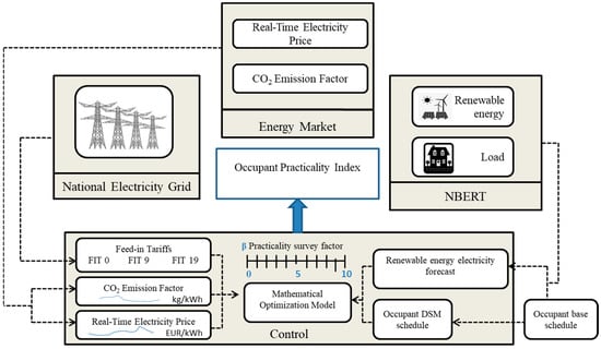
Figure 6.
Renewable microgrid practicality process overview showing the relationships and interconnections of the simulations carried out in the research.
3. Results and Discussion
3.1. Renewable Energy Generation and Supply
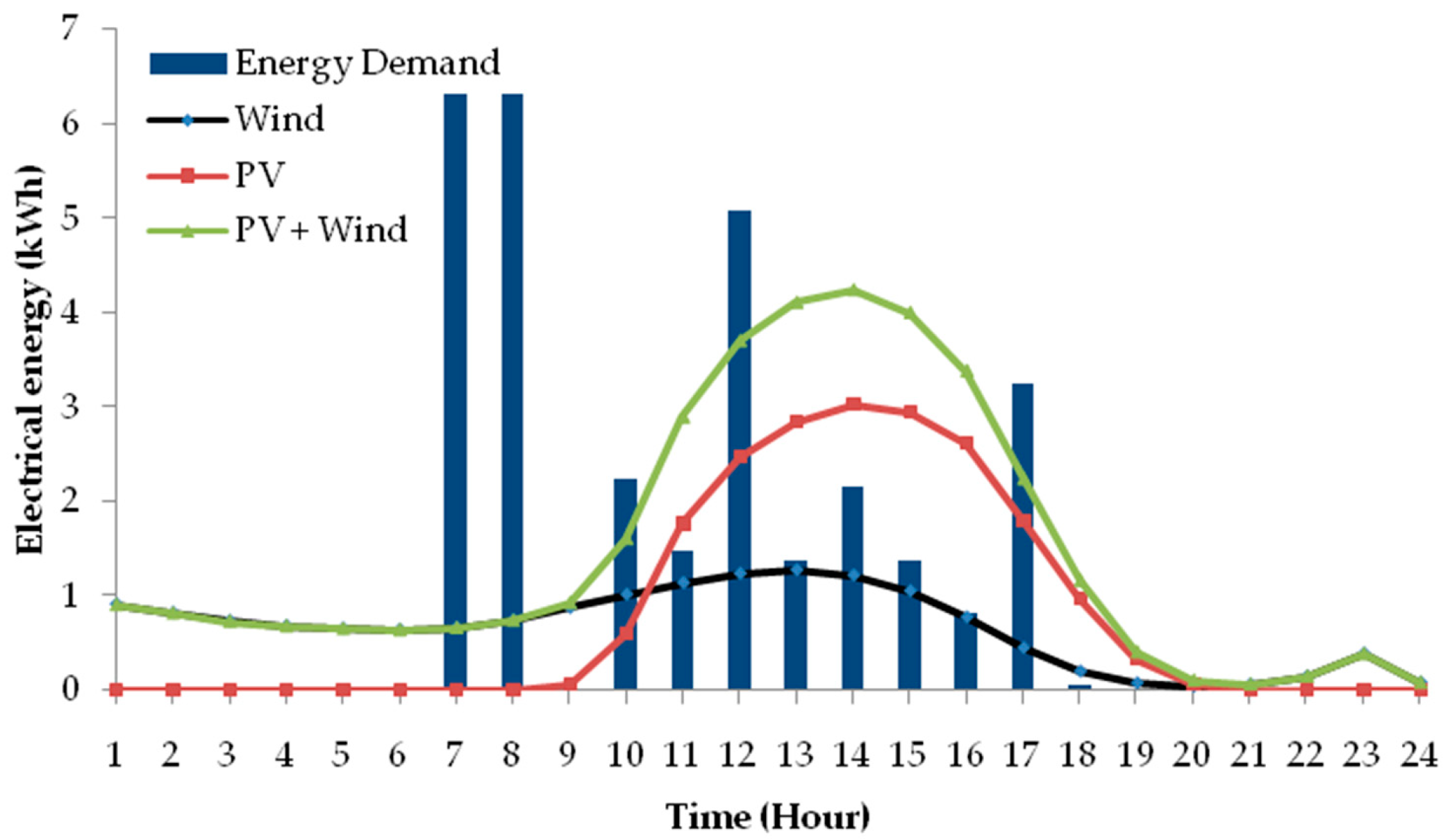
The results of the REµG energy output were averaged across the months of January, February, March, April, May, July and September for 2013. The average REµG energy outputs were 35.10 kWh, 54.47 kWh and 89.58 kWh for PV, wind and PV + wind, respectively. Figure 7 shows the mean hourly PV, wind turbine and PV + wind turbine energy outputs along with the corresponding hourly electricity demand of occupant A averaged across the five-day work week for schedule 0. Figure 8 shows the same data for schedule 1. Similar figures for schedules 2 to 5 are presented in Appendix B Figure A2, Figure A3, Figure A4 and Figure A5, and a supporting dataset has been included in the Supplementary Materials.

Figure 7.
Mean hourly PV energy output (kWh), mean hourly wind turbine energy output (kWh) and mean hourly PV + wind energy output (kWh) with corresponding total hourly energy demand (kWh) of occupant A for schedule 0.
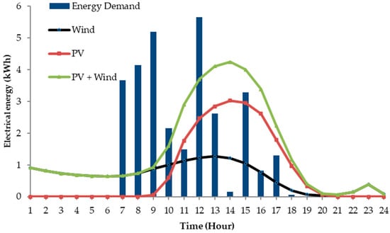
Figure 8.
Mean hourly PV energy output (kWh), mean hourly wind turbine energy output (kWh) and mean hourly PV + wind energy output (kWh) with corresponding total hourly energy demand (kWh) of occupant A for schedule 1.
Table 3 presents a summary of the energy use and supply for the NBERT building over the study period. For the generated DSM schedules and the load priority control, the PV configuration had the highest percentage of renewable energy use in schedule 2 (54%). The PV + wind configuration had the lowest percentage of renewable energy use in schedule 5 at 24%. This resulted in the PV configuration exporting the lowest percentage (of generated energy) to the national smart grid at 46% (schedule 2) and the PV + wind configuration having the highest exported energy percentage of 76% (schedule 5). As the electricity demand was from occupants of an office building, most of their electricity requirements were during daytime hours. Subsequently, the electricity demand was more in sync with the PV power output profile (Figure 7 and Figure 8). The DSM schedules were unique for all occupants; therefore, the schedule with the minimum and maximum amounts of renewable energy used and exported varied per occupant depending on their fixed work patterns. However, the PV configuration had the highest percentages of renewable energy used across all occupants and all DSM schedules. The PV + wind configuration resulted in the highest percentages of the occupants’ electricity requirements being supplied by renewable sources in schedule 3 (91%). This resulted in the NBERT building requiring only 9% of its electricity from the national smart grid. Across all schedules for the load priority control, the PV + wind configuration resulted in the highest avoided CO2 (91%) for both schedules 2 and 3, with values of 11.8 kg of CO2 and 12.1 kg of CO2, respectively. Alternatively, the PV configuration resulted in the lowest reductions in CO2 avoided (44%) for schedule 5.
Table 3.
Renewable energy used by National Build Energy Retrofit Test-bed occupants (kWh, %), renewable energy exported to the national smart grid (kWh, %), energy supplied by real-life renewable energy microgrid (REµG) (kWh, %), energy demand supplied by national smart grid (kWh, %), avoided CO2 by REµG (Kg of CO2, %) for the four REµG configurations, the base schedule (schedule 0) and the five demand-side management schedules (schedules 1–5) for occupant A.
3.2. Renewable Energy Microgrid Control Results
For the no REµG configuration (Section 2.5), schedule 2 had the highest MBC and lowest CQ (Section 2.6), with average values of EUR 5.97 and 11.72 kg, respectively (Table 4). This was because schedule 2 shifted the working hours of the NBERT office occupants into evening hours, where the RTP energy prices peaked and grid emissions were at a minimum (Figure 4). Therefore, when using the grid priority control, shifting occupant working hours to the evening is expected to increase the monetary cost of energy and reduce the CO2 cost. Subsequently, schedule 2 had the highest AC across all FITs and REµG configurations, with average values ranging from EUR −7.39 to EUR 3.55. Concurrently, schedule 5 had the lowest AC for all FITs and REµG configurations, with average values ranging from EUR −7.80 to EUR 3.12 (Table 5). Low AC implies more earnings from the FITs; hence, a negative AC means profit. As outlined in Section 2.4, FIT0 is not applicable when using grid priority control because it will imply selling electricity to the national smart grid at 0 cents with zero income and no economic benefit, thereby equivalent to a no REµG configuration. Therefore, Table 5 does not have FIT0 represented. Notably in Table 4 below, the no REµG configuration and grid priority control had the same MBCs. This is because when using either no REµG or grid priority control, the entire electricity requirement of the NBERT occupants was met by the national smart grid. The results in Table 4 outline that for both the no REµG configuration and grid priority control, schedule 1 and schedule 5 had the lowest MBC at EUR 5.56. As outlined in Section 2.2, schedules 1 and 5 were designed to avoid the periods when energy monetary costs are higher, hence why they have the lowest MBC when using the no REµG configuration or grid priority control.
Table 4.
Monetary buying cost (EUR) for the no renewable energy microgrid (no REµG) configuration, grid priority control and load priority control with no feed-in tariff (FIT0). Data are averaged across all occupants for the base schedule (schedule 0) and five demand-side management schedules (schedules 1–5).
Table 5.
Aggregate cost (EUR) when using grid-priority microgrid control logic averaged across all occupants for the base schedule (schedule 0) and five demand-side management schedules (schedules 1–5) for feed-in tariff (FIT) structures FIT9 and FIT19. FIT0 is not included, as it is equivalent to a no REµG configuration in terms of AC for the grid priority control.
When using grid priority control, AC values are driven by the MBC. This is because the REµG income is the same value for all schedules, as all the electricity from the renewable energy sources was sold to the national smart grid. Conversely, when using load priority control, only the excess electricity that is not consumed by the NBERT office occupants was sold to the national smart grid. Hence, the AC is driven by the REµG income when using load priority control and the amount of excess electricity that is not consumed by the occupants determines the REµG income. In summary, when using load priority control, the AC decreases as the REµG income increases, whereas when using grid priority control, the AC increases as the MBC increases.
For load priority control under schedule 1, the PV configuration had the highest MBC value of EUR 2.43 (Table 4). As shown in Figure 8, schedule 1 shifted the working hours of the NBERT occupants into the early hours, away from the solar peak period. Subsequently, the MBC is highest in this scenario because the renewable REµG controller supplied lower energy, thereby leading to more energy being bought from the national smart grid. Considering only the DSM schedules, schedule 3 under the PV + wind configuration had the minimum MBC value of EUR 0.36 (Table 4). Schedule 3 generally had the lowest AC across all FITs and REµG configurations, with values ranging from EUR −4.27 to EUR 1.94 except for schedule 1 for FIT19, which had EUR −2.78 and EUR −8.95 for the wind and PV + wind configurations, respectively (Table 6). As seen in Table 7, schedule 2 had the highest percentage of avoided CO2 for the PV configuration (68%), while schedule 3 had the highest rate of avoided CO2 for the wind and PV + wind configurations (73% and 93%, respectively). Schedule 5 had the lowest percentage of avoided CO2 for all REµG configurations, with values of 53%, 67% and 81% for PV, wind and PV + wind REµG configurations, respectively. This was because schedule 5 shifted the load profiles of the occupants to early morning and late evening periods, which corresponded to periods when carbon factors were higher (Figure 4). Schedule 3 was generated to create a balance between working in the early morning hours and working late in the evening. Therefore, schedule 3 had more of its energy demand supplied by the REµG during the daytime, thereby requiring comparatively less energy to be bought from the national smart grid, which generally resulted in higher percentages of avoided CO2.
Table 6.
Aggregate cost (EUR) when using load-priority microgrid control logic averaged across all occupants for the base schedule (schedule 0) and five demand-side management schedules (schedules 1–5) for all examined feed-in tariff structures.
Table 7.
Avoided CO2 (%) by load priority control for all the renewable energy microgrid configurations.
3.3. Occupant Practicality and Electricity Costs
It is important to note that price-based DSM refers to the selection of the most cost-effective DSM schedule and not the most practical. While the practicality of a particular schedule does not change, the corresponding cost effectiveness of the schedule will change as it is affected by factors such as the REµG configuration, FIT, controller and so on. Therefore, the practicality of price-based DSM will differ based on these factors. From the results presented in Table 8, it was found that there was a general negative correlation between the practicality of DSM schedules and MBC in configurations where there was no REµG or when using grid priority control. However, when the REµG was introduced with load priority control, the correlation between DSM schedule practicality and MBC became positive. This is because the REµG introduces energy from sources such as PV power that are available during the daytime, which coincides with periods when the building occupants are at work. The degree of negativity, positivity and strength of the correlation varies per individual due to their preferred working hours. Load priority configurations that supported greater self-consumption of REµG-generated electricity showed a shift from negative to positive correlations between practicality and MBC. For example, occupant A had a correlation shift from −0.35 with the no REµG configuration/grid priority control to 0.94 for the load-priority PV configuration. This was due to most of the electricity demand being met by PV power and a reduced requirement for purchasing electricity at a high cost during the day. For the no REµG configurations, occupant F had the strongest negative correlation between practicality and MBC, with a strong negative correlation of −0.76. In contrast, occupant G had the strongest positive correlation between practicality and MBC of 0.32. The results of the correlation between practicality and MBC for no REµG configurations and grid priority control are the same because MBC is the same for both scenarios, as previously stated in Section 2.5.
Table 8.
Pearson correlation coefficients between each occupant’s practicality and monetary buying cost (MBC) across no renewable energy microgrid (no REµG), PV, wind, and PV + wind microgrid configurations for grid priority and load priority controls with no feed-in tariff (FIT0).
The introduction of REµG energy supply to the building made DSM schedules more practical (in terms of MBC), with an average of 0.69, 0.62 and 0.75 for PV, wind and PV + wind, respectively. This is because the occupants’ base schedule was better aligned with electricity prices, as RTP is based on the national smart grid energy demand, which is heavily influenced by the daily schedules of the Irish population. This leads to price-based DSM schedule cost savings having higher impracticality when using the grid priority control. However, introducing the load-priority microgrid control made cost savings from the price-based DSM schedules more practical with respect to the MBC. The increase in practicality of price-based DSM schedules through the introduction of the REµG energy supply was more pronounced for PV compared with wind power.
In summary, when there was no REµG, there was a weak or negative correlation between the practicality of DSM schedules and the price of electricity. Alternately, when REµG was added, there was a greater amount of free renewable energy supplied in the middle of the day. For most people, it was more practical to come to work in the middle of the day than to come early in the morning or late in the evening. Therefore, the correlation between the practicality of DSM schedules and the price of electricity changes from negative to positive.
Table 9 below shows that the introduction of FIT9 resulted in a reduced correlation between the practicality of DSM schedules and MBC, while the introduction of FIT19 resulted in a further reduced correlation between practicality and MBC. Therefore, it was found that the correlation between practicality and MBC generally became weaker when FITs were introduced to the REµG. This was because the benefit of self-consumption of renewable energy decreased as the export value of the renewable energy increased. The income generated from daytime excess REµG energy, which was sold to the grid when using load-priority microgrid control, led to lower ACs. The introduction of REµG into the energy supply chain of the NBERT building did not indicate much of a difference in the practicality of DSM schedule correlation with respect to CQ (Table 10). This was potentially due to the NBERT building occupants working during the daytime, since CQ is higher during the early morning and night hours and is not driven by energy demand.
Table 9.
Pearson correlation coefficients between each occupant’s practicality and aggregate credit (AC) across PV, wind and PV + wind renewable energy microgrid configurations and all examined feed-in tariff (FIT) structures when using load priority.
Table 10.
Pearson correlation coefficient between occupant practicality of demand-side management schedule and carbon quantity (CQ) for PV, wind, PV + wind and no renewable energy microgrid (no REµG) configurations.
3.4. Occupant A as a Case Study Reference for Practicality and Energy Costs
To investigate the relationship between practicality and energy costs in more detail, the following section focuses on results for occupant A as a case study. As seen in Table 8 and Table 10 above, the practicality correlation with the electricity MBC and CQ for occupant A are −0.35 and 0.99, respectively, for no REµG. The strength of these correlations can be seen in Figure 9a,b below. Figure 9a shows that the linear trend graph of practicality is in the opposite direction of the linear trend graph of the MBC and that there is a moderate negative correlation between them. However, in Figure 9b, it is noticeable that the linear trend graph of practicality is in the same direction as the linear trend graph of CQ (kg) and that there is a strong positive correlation between them. Figure 9a,b, Figure 10a,b, Figure 11a,b, Figure 12a,b and Figure 13a,b are ranked based on the practicality range (0 to 1) and not in order of the schedules (0 to 5).
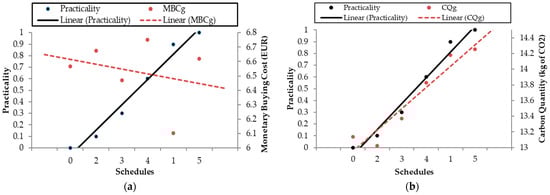
Figure 9.
(a) Linear trend graph of correlation between practicality and monetary buying cost (EUR) when using the no renewable energy microgrid (no REµG) configuration or grid priority control for occupant A (MBCg) (feed-in tariff not applicable); (b) linear trend graph of correlation between practicality and carbon quantity (kg) for the no REµG configuration or grid priority control for occupant A (CQg).
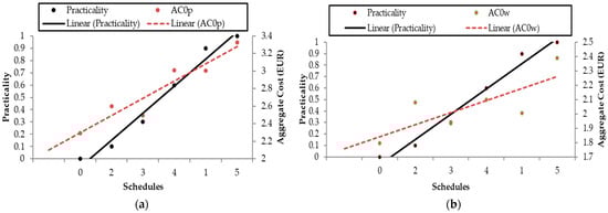
Figure 10.
(a) Linear trend graph of correlation between practicality and aggregate cost (EUR) when using the load priority control for the PV renewable energy microgrid (REµG) configuration for occupant A with no feed-in tariff (FIT0) (AC0p); (b) linear trend graph of correlation between practicality and aggregate cost (EUR) when using the load priority control for the wind REµG configuration for occupant A at FIT0 (AC0w).
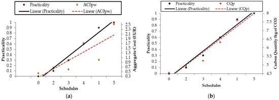
Figure 11.
(a) Linear trend graph of correlation between practicality and aggregate cost (EUR) when using the load priority control for the PV + wind renewable energy microgrid (REµG) configuration for occupant A with no feed-in tariff (FIT0) (AC0pw); (b) linear trend graph of correlation between practicality and carbon quantity (kg) when using the load-priority control application for the PV REµG configuration for occupant A (CQp).
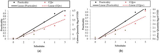
Figure 12.
(a) Linear trend graph of correlation between practicality and carbon quantity (kg) when using the load priority for wind for occupant A (CQw); (b) linear trend graph of correlation between practicality and carbon quantity (kg) when using the load priority control for the PV + wind renewable energy microgrid (REµG) configuration for occupant A (CQpw).
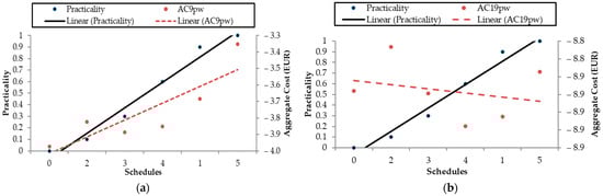
Figure 13.
(a) Linear trend graph of correlation between practicality and aggregate cost (EUR) when using the load-priority microgrid control for the PV + wind renewable energy microgrid (REµG) configuration for occupant A at 0.09 EUR/kWh feed-in tariff (FIT9) (AC9pw); (b) linear trend graph of correlation between practicality and aggregate cost (EUR) when using the load-priority microgrid control for the PV + wind REµG configuration for occupant A at 0.19 EUR/kWh feed-in tariff (FIT19) (AC19pw).
Figure 10a,b and Figure 11a represent the linear trend graphs between practicality and MBC when using the load priority control for PV, wind and PV + wind configurations, respectively. From Table 8 above, the correlation coefficients between practicality and MBC when using load priority control for PV, wind and PV + wind configurations were 0.94, 0.71 and 0.80, respectively. This implied that introducing a REµG changed the DSM schedules from not being practical to being practical with respect to the MBC. As discussed in Section 3.3, this was because renewable energy sources such as PV power were available during the daytime, which was also when the NBERT occupants were available to work in the office. This also corresponds with electricity RTP generally having higher prices during the day compared to the late evening and early morning. Furthermore, this demonstrates why the PV configuration had the most substantial correlation (0.94) between practicality and MBC for occupant A. Figure 11b and Figure 12a,b represent the linear trend graphs between practicality and CQ when using the load priority control for PV, wind and PV + wind configurations, respectively. From Table 10 above, the correlation coefficients for the same were 0.99, 0.93 and 0.90, respectively. Comparing these values to the 0.99 correlation value obtained between practicality and CQ when using the no REµG configuration suggests that the CQ content of electricity slightly affects the practicality of the DSM schedules. Figure 13a represents the linear trend graphs between practicality and AC for the load-priority microgrid control at FIT9 for the PV + wind configuration, while Figure 13b represents the linear trend graphs between practicality and AC for the load-priority microgrid control at FIT19 for the PV + wind REµG configuration. From Table 9 above, the correlation coefficients for the same were 0.83 and −0.35, respectively. From Section 3.3 above, it has been detailed that the introduction of the FIT9 and FIT19 structures resulted in a reduction in practicality correlations; this can be seen by comparing the AC correlation figures when using the load-priority microgrid control (Figure 13a,b) with MBC correlation figures (Figure 10a,b and Figure 11a).
In summary, reducing energy costs via price-based DSM was found to be impractical when no renewable energy source was utilized in conjunction with price-based DSM. Subsequently, the introduction of renewable energy increased the practicality of priced-based DSM scenarios. However, when FITs for exporting renewable energy to the grid were introduced, this had a negative impact on the relationship between practicality and the financial benefits of priced-based DSM. In general, the employment of DSM to reduce the CQ of electricity usage had a positive effect on practicality for the occupants.
3.5. General Discussion
This paper investigated the level of practicality for electricity users to partake in specific price-based DSM schedules. Ten occupants of the NBERT building were used as a case study with one base schedule and five DSM schedules, making a total of six unique schedules per occupant. Three microgrid controllers were explored, namely no REµG, grid priority and load priority. Electricity was bought at RTP, and CO2 emission factors were utilized to analyze the CO2 offsets. Three FITs, FIT0, FIT9 and FIT19, were used to evaluate the practicality of the DSM schedules. Our results can be divided into three main stages:
- Stage one: This involves the no REµG configuration and grid priority control scenarios, where all the electricity required by the building occupants was bought from the national smart grid. No renewable energy was supplied to the NBERT building when using the no REµG configuration. Renewable energy was supplied to the NBERT building when using grid priority control; however, the entire renewable energy source was sold to the national grid through FITs in stage three.
- Stage two: Load priority control was used to prioritize the electricity supply to the NBERT building occupants.
- Stage three: FITs were introduced for electricity exported to the national smart grid.
At stage one, it was found that money could be saved by changing the occupant schedules with price-based DSM. This has been reported by several studies [6,27,28,29,30]; however, this research showed that price-based DSM is very impractical for building occupants. This corroborates with the findings of Wallin et al. [3], who reported that household energy users had low willingness to participate in DSM programs despite being offered economic compensation. The shape of the national smart grid is structured based on people’s electricity usage patterns; electrical appliances are used by people at home in the mornings, such as electric showers, tea- and coffee-making machines. Office users also use equipment in the morning and daytime, such as photocopying machines, laptops and kettles. This can be seen in Figure 4, where the RTP tariff starts to increase in the morning and evening before and after regular work hours. Electricity costs also increase in the late evenings when people return to their homes and use more electrical equipment such as ovens, televisions and showers. Subsequently, the RTP profile is driven by people’s practical needs. Therefore, this explains our findings for the no REµG configurations and grid priority control, which indicate that DSM schedules relative to RTP tariffs are less practical for NBERT office occupants. This can be seen in Figure 9a, where the linear trend of practicality of the DSM schedule is in the opposite direction of the linear trend of the MBC. This can also be seen in Table 8, where the mean correlation between the practicality of the DSM schedule and the RTP MBC was −0.27. However, for no REµG configurations and grid priority control, it was found that relative to the carbon quantity, DSM schedules are more practical. This can be seen in Figure 9b, where the linear trend for practicality of the DSM schedule is in the same direction as the linear trend of CQ.
For grid priority control, the results show that it is less practical for people to use DSM schedules, which is expected for people working in an office building, as their natural schedule aligns with the price of electricity. When we generated work schedules for the NBERT building occupants that had a greater focus on saving money through DSM, this further reduced costs but pushed them further from their base schedule. Therefore, the use of price-based DSM became increasingly less practical. For example, Figure 9a shows that changing occupant A’s schedule via price-based DSM is not practical when there is no REµG and all energy is supplied from the national smart grid. Park [31] developed a human comfort-based control approach for DR participation of households to reduce energy user response fatigue. A similar approach may be valid for price-based DSM, based on the observed negative correlation between practicality and cost savings.
At stage two, the study showed the level of practicality of adopting the most cost-effective DSM schedules changes considerably with the addition of a REµG to the NBERT building. The practicality of price-based DSM was inversed as the most practical price-based DSM schedule became the most cost effective, as shown in Figure 9a, Figure 10a,b and Figure 11a. This is because the renewable energy sources added to the NBERT building drove down the MBC and CQ of occupants’ energy use. The availability of renewable energy sources during the daytime, particularly PV power, played a significant role in making the most practical DSM schedule more cost effective. More renewable power was available during the daytime, and therefore, more REµG power was utilized by the building occupants instead of buying electricity from the national smart grid, which was more expensive during this time.
The increase in practicality through the introduction of the REµG was more pronounced for the PV configuration in comparison to the wind turbine configuration. This is because during daytime hours, PV power is typically more abundant than wind turbine-generated electricity, and the occupants of the NBERT building also work in the office primarily at this time. Hence, PV generation is more aligned with the work schedules of the office occupants. This is supported by the findings of Rotas et al. [32], who outlined the potential for a 60% reduction in the annual electricity load using PV microgeneration integrated with an office building in Wales. The addition of a REµG to the NBERT building energy mix made a substantial difference and ultimately made price-based DSM more practical.
At stage three of the results, adding different FITs had a negative effect on the practicality of DSM with a REµG, especially when the FIT value increased. This can be seen in Figure 13b, Figure 14b and Figure 15b, which show that DSM was less practical when higher FITs were introduced to the microgrid. The correlation values in Table 9 showed that the introduction of FIT9 at 0.09 EUR/kWh had a low impact on the practicality of using price-based DSM. The practicality decreased substantially when the FIT was increased to 0.19 EUR/kWh, with more substantial deviations in correlation. This is because a higher FIT results in more revenue from exporting to the national smart grid, which drives down the AC of price-based DSM.
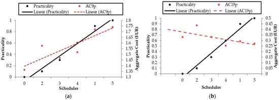
Figure 14.
(a) Linear trend graph of correlation between practicality and aggregate cost (EUR) when using the load-priority microgrid control for PV renewable energy microgrid (REµG) configuration for occupant A at 0.09 EUR/kWh feed-in tariff (FIT9) (AC9p); (b) Linear trend graph of correlation between practicality and aggregate cost (EUR) when using the load-priority microgrid control for PV renewable energy microgrid (REµG) configuration for occupant A at 0.19 EUR/kWh feed-in tariff (FIT19) (AC19p).
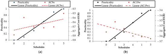
Figure 15.
(a) Linear trend graph of correlation between practicality and aggregate cost (EUR) when using the load-priority microgrid control for the wind renewable energy microgrid (REµG) configuration for occupant A at 0.09 EUR/kWh feed-in tariff (FIT9) (AC9w); (b) linear trend graph of correlation between practicality and aggregate cost (EUR) when using the load-priority microgrid control for the wind REµG configuration for occupant A at 0.19 EUR/kWh feed-in tariff (FIT19) (AC9w).
In summary, the results showed that implementing price-based DSM to reduce energy costs was not practical for the occupants of the NBERT office building in a RTP tariff scenario with no REµG. However, introducing a REµG made price-based DSM much more practical, as the daytime DSM schedules better synchronized the daily energy demand with the REµG energy output. The introduction of FIT9 and FIT19 reversed some of these results and made price-based DSM less practical, as higher FITs created a financial incentive to utilize less REµG energy output and to shift electricity consumption to less practical periods. Therefore, it may be less logical to implement price-based DSM in an environment with high FITs as the cost-saving benefits are reduced.
4. Conclusions
This body of work quantified the practicality of price-based DSM relative to monetary and CO2 costs using an office building with an integrated REµG as a case study. The main findings of this study are as follows:
- The main factors that contributed to practicality of price-based DSM were RTP profile, REµG controller logic and FIT.
- In scenarios that excluded onsite REµG generation, price-based DSM schedules tended to push occupant energy consumption away from peak periods to reduce costs. This had a negative impact on practicality for the occupants, as it deviated their work schedule further away from the typical working day.
- There was a negative correlation (r = −0.27) between practicality and the savings produced by price-based DSM schedules (monetary cost (EUR)) when the electricity demands of the building were met solely by the grid.
- There was a general positive correlation (r = 0.39) between the practicality of price-based DSM relative to reducing the CQ.
- REµG configurations that included PV power had the most substantial positive impact on the correlation between aggregate cost and practicality (r = 0.69–0.75) due to PV generation coinciding with the most practical price-based DSM schedules and the most expensive electricity prices.
- Cost savings (EUR 0.41) per day were achieved by implementing price-based DSM schedules for occupants of an office building without an REµG. However, a very low level of practicality was associated with the cost savings achieved.
- The use of price-based DSM was most practical when no or low-rate FITs were available. However, when higher-rate FITs were available, price-based DSM was less practical (r = 0.15–0.64).
To conclude, the incorporation of onsite renewable energy generation with price-based DSM had a positive impact on occupant practicality. Conversely, the introduction of a feed-in tariff with a renewable energy microgrid made price-based DSM less practical.
Supplementary Materials
The following supporting information can be downloaded at: https://www.mdpi.com/article/10.3390/su16188120/s1, Supplementry energy demand_RE output dataset.xlsx.
Author Contributions
Conceptualization, D.A.A. and M.D.M.; methodology, D.A.A. and M.D.M.; software, D.A.A., P.S. and M.D.M.; investigation, D.A.A. and D.J.M.; data curation D.A.A. and P.S.; writing—original draft preparation, D.A.A., M.D.M. and D.J.M.; writing—review and editing, D.J.M. and M.D.M.; visualization, D.A.A., P.S., D.J.M. and M.D.M.; supervision, M.D.M. and D.J.M. All authors have read and agreed to the published version of the manuscript.
Funding
This research received no external funding.
Institutional Review Board Statement
Munster Technological University’s Human Research Ethics Committee has undertaken a research ethical review of the study and is satisfied that research ethical considerations have been addressed and has granted permission for the study to proceed (Approval No: MTU-HREC-FER-23-037-A). The study was conducted in accordance with the Declaration of Helsinki and approved by the Ethics Committee of Munster Technological University (HREC-FER-23-037, 29/01/24) for studies involving humans.
Informed Consent Statement
Informed consent was obtained from all subjects involved in the study. Written informed consent has been obtained from the participants of the study to publish this paper.
Data Availability Statement
Dataset available on request from the authors.
Conflicts of Interest
The authors declare no conflicts of interest.
Nomenclature
| DSM | Demand-side management |
| DR | Demand response |
| NBERT | National Build Energy Retrofit Test-bed |
| REµG | Renewable energy microgrid |
| RTP | Real-time pricing (EUR/kWh) |
| FIT | Feed-in tariff (EUR/kWh) |
| OED | Base occupant energy demand (kWh) |
| WED | Energy demand for an occupant’s workstation (kWh) |
| TCED | Energy demand for an occupant making tea or coffee (kWh) |
| DSTREM | Decision support tool for renewable energy microgrids |
| RTPET | Real-time pricing electricity tariff (EUR/kWh) |
| FIT0 | Feed-in tariff (0 EUR/kWh) |
| FIT9 | Feed-in tariff (0.09 EUR/kWh) |
| FIT19 | Feed-in tariff (0.19 EUR/kWh) |
| MBC | Monetary buying cost (EUR) |
| CQ | Carbon quantity (kg) |
| AC | Aggregate cost (EUR) |
| EsG | Electricity supplied by the national smart grid (kW) |
| ET | Electricity tariff (EUR/kW) |
| CEF | CO2 emission factor (kg/kWh) |
| Ereq | Total electricity requirement of the building occupant (kW) |
| µGinc | Daily REμG monetary income (EUR) |
| Eex | Energy exported by the REµG (kWh) |
| AC0p | Aggregate cost at PV configuration (FIT0) (EUR) |
| AC0pw | Aggregate cost at PV + wind configuration (FIT0) (EUR) |
| AC0w | Aggregate cost at wind configuration (FIT0) (EUR) |
| AC19p | Aggregate cost at PV configuration (FIT19) (EUR) |
| AC19pw | Aggregate cost at PV + wind configuration (FIT19) (EUR) |
| AC19w | Aggregate cost at wind configuration (FIT19) (EUR) |
| AC9p | Aggregate cost at PV configuration (FIT9) (EUR) |
| AC9pw | Aggregate cost at PV + wind configuration (FIT9) (EUR) |
| CQg | Carbon quantity at no REµG configuration and grid priority control (kg) |
| CQp | Carbon quantity (load priority control at PV configuration) (kg) |
| CQpw | Carbon quantity (load priority control at PV + wind configuration) (kg) |
| CQw | Carbon quantity (load priority control at wind configuration) (kg) |
Appendix A
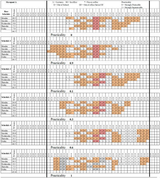
Figure A1.
Base work schedule (0) and generated schedules (1–5) for occupant A, with practicality ratings and daily working hours displayed. W hours denotes daily working hours, IO denotes the occupant was in the office with electrical devices switched on IO* denotes the occupant was in the office and made a cup of tea using the hot kettle, L denotes the occupant left the office and went to the lecture hall, and the electrical devices at his or her workstation were on standby mode, and OF denotes the occupant was out of the office for lunch break or personal reasons, and the electrical devices were on standby mode.
Appendix B
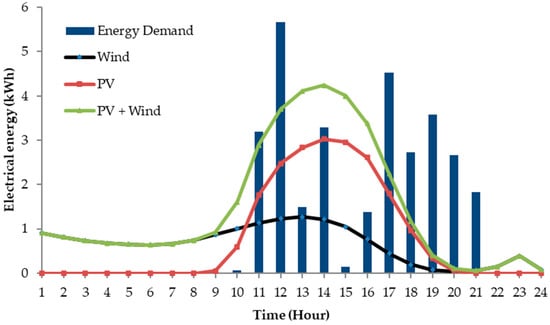
Figure A2.
Mean hourly PV energy output (kWh), mean hourly wind turbine energy output (kWh) and mean hourly PV + wind energy output (kWh) with corresponding total hourly energy demand (kWh) of occupant A for schedule 2.
Figure A2.
Mean hourly PV energy output (kWh), mean hourly wind turbine energy output (kWh) and mean hourly PV + wind energy output (kWh) with corresponding total hourly energy demand (kWh) of occupant A for schedule 2.
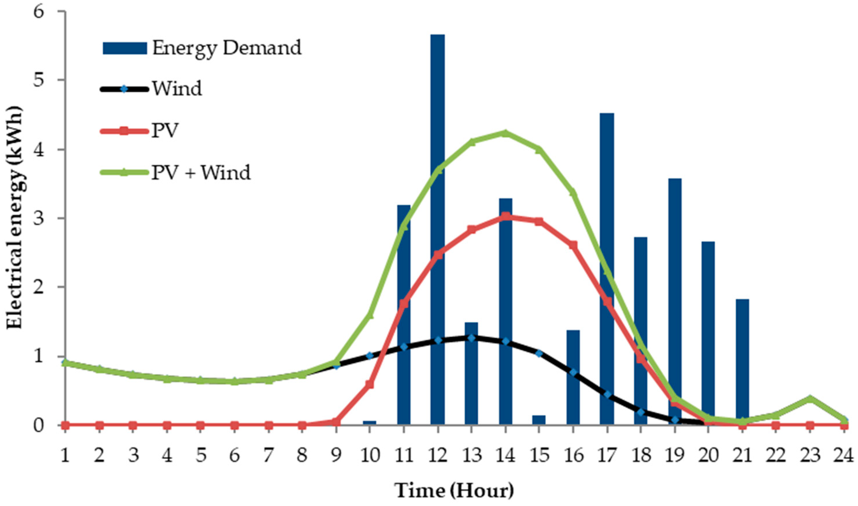
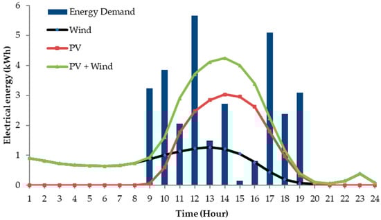
Figure A3.
Mean hourly PV energy output (kWh), mean hourly wind turbine energy output (kWh) and mean hourly PV + wind energy output (kWh) with corresponding total hourly energy demand (kWh) of occupant A for schedule 3.
Figure A3.
Mean hourly PV energy output (kWh), mean hourly wind turbine energy output (kWh) and mean hourly PV + wind energy output (kWh) with corresponding total hourly energy demand (kWh) of occupant A for schedule 3.

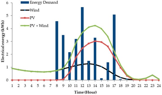
Figure A4.
Mean hourly PV energy output (kWh), mean hourly wind turbine energy output (kWh) and mean hourly PV + wind energy output (kWh) with corresponding total hourly energy demand (kWh) of occupant A for schedule 4.
Figure A4.
Mean hourly PV energy output (kWh), mean hourly wind turbine energy output (kWh) and mean hourly PV + wind energy output (kWh) with corresponding total hourly energy demand (kWh) of occupant A for schedule 4.

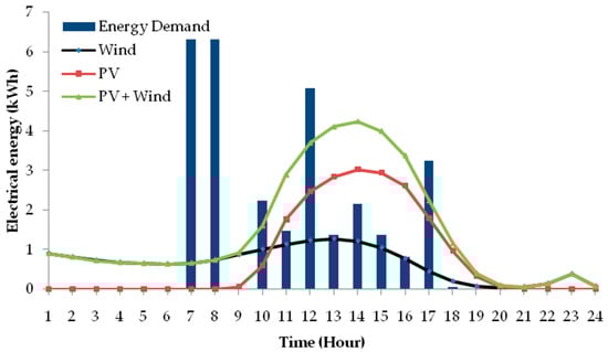
Figure A5.
Mean hourly PV energy output (kWh), mean hourly wind turbine energy output (kWh) and mean hourly PV + wind energy output (kWh) with corresponding total hourly energy demand (kWh) of occupant A for schedule 5.
Figure A5.
Mean hourly PV energy output (kWh), mean hourly wind turbine energy output (kWh) and mean hourly PV + wind energy output (kWh) with corresponding total hourly energy demand (kWh) of occupant A for schedule 5.
References
- Walker, A. Exploring the Limits of Demand Side Management. Master’s Thesis, University of Strathclyde, Glasgow, UK, 2006. Available online: https://citeseerx.ist.psu.edu/document?repid=rep1&type=pdf&doi=bd46661db7c87d582fdb7ad141f435d3530d6c63 (accessed on 5 November 2023).
- Jabir, H.J.; Teh, J.; Ishak, D.; Abunima, H. Impacts of Demand-Side Management on Electrical Power Systems: A Review. Energies 2018, 11, 1050. [Google Scholar] [CrossRef]
- Wallin, F.; Torstensson, D.; Kovala, T.; Sandberg, A. Using an Energy Intervention Framework to Evaluate End-User Willingness to Participate in Demand- Response Activities. In Proceedings of the 2016 IEEE Power and Energy Society General Meeting (PESGM), Boston, MA, USA, 17–21 July 2016. [Google Scholar] [CrossRef]
- Asaleye, D.A.; Murphy, M.D. Monetary Savings Produced by Multiple Microgrid Controller Configurations in a Smart Grid Scenario. In Proceedings of the 2016 IEEE International Energy Conference, ENERGYCON, Leuven, Belguim, 4–8 April 2016. [Google Scholar]
- Kanakadhurga, D.; Prabaharan, N. Demand Side Management in Microgrid: A Critical Review of Key Issues and Recent Trends. Renew. Sustain. Energy Rev. 2022, 156, 111915. [Google Scholar] [CrossRef]
- Zhang, J.; Wu, J.; Fu, L.; Wu, Q.; Huang, Y.; Qiu, W.; Ali, A.M. Energy Optimization of the Smart Residential Electrical Grid Considering Demand Management Approaches. Energy 2024, 300, 131641. [Google Scholar] [CrossRef]
- Sun, H.; Sun, X.; Kou, L.; Zhang, B.; Zhu, X. Optimal Scheduling of Park-Level Integrated Energy System Considering Ladder-Type Carbon Trading Mechanism and Flexible Load. Energy Rep. 2023, 9, 3417–3430. [Google Scholar] [CrossRef]
- Xie, T.; Ma, K.; Zhang, G.; Zhang, K.; Li, H. Optimal Scheduling of Multi-Regional Energy System Considering Demand Response Union and Shared Energy Storage. Energy Strategy Rev. 2024, 53, 101413. [Google Scholar] [CrossRef]
- Roshan, A.; Ganga, D. Intelligent Categorization and Interactive Mechanism for Smart Demand Side Management of Residential Consumers. Sustain. Energy Grids Netw. 2024, 37, 101255. [Google Scholar] [CrossRef]
- Menos-Aikateriniadis, C.; Lamprinos, I.; Georgilakis, P.S. Particle Swarm Optimization in Residential Demand-Side Management: A Review on Scheduling and Control Algorithms for Demand Response Provision. Energies 2022, 15, 2211. [Google Scholar] [CrossRef]
- Pascual, J.; Arcos-Aviles, D.; Ursúa, A.; Sanchis, P.; Marroyo, L. Energy Management for an Electro-Thermal Renewable–Based Residential Microgrid with Energy Balance Forecasting and Demand Side Management. Appl. Energy 2021, 295, 117062. [Google Scholar] [CrossRef]
- Zhang, D.; Shah, N.; Papageorgiou, L.G. Efficient Energy Consumption and Operation Management in a Smart Building with Microgrid. Energy Convers. Manag. 2013, 74, 209–222. [Google Scholar] [CrossRef]
- Samadi, P.; Mohsenian-Rad, A.-H.; Schober, R.; Wong, V.W.S.; Jatskevich, J. Optimal Real-Time Pricing Algorithm Based on Utility Maximization for Smart Grid. In Proceedings of the First IEE International Conference on Smart Grid Communications (SmartGridComm), Gaithersburg, MD, USA, 4–6 October 2010. [Google Scholar]
- Missaoui, R.; Joumaa, H.; Ploix, S.; Bacha, S. Managing Energy Smart Homes According to Energy Prices: Analysis of a Building Energy Management System. Energy Build. 2014, 71, 155–167. [Google Scholar] [CrossRef]
- Fell, M.J.; Shipworth, D.; Huebner, G.M.; Elwell, C.A. Public Acceptability of Domestic Demand-Side Response in Great Britain: The Role of Automation and Direct Load Control. Energy Res. Soc. Sci. 2015, 9, 72–84. [Google Scholar] [CrossRef]
- Joe-Wong, C.; Sen, S.; Ha, S.; Chiang, M. Optimized Day-Ahead Pricing for Smart Grids with Device-Specific Scheduling Flexibility. IEEE J. Sel. Areas Commun. 2012, 30, 1075–1085. [Google Scholar] [CrossRef]
- Gao, J.; Ma, Z.; Guo, F. The Influence of Demand Response on Wind-Integrated Power System Considering Participation of the Demand Side. Energy 2019, 178, 723–738. [Google Scholar] [CrossRef]
- D’hulst, R.; Labeeuw, W.; Beusen, B.; Claessens, S.; Deconinck, G.; Vanthournout, K. Demand Response Flexibility and Flexibility Potential of Residential Smart Appliances: Experiences from Large Pilot Test in Belgium. Appl. Energy 2015, 155, 79–90. [Google Scholar] [CrossRef]
- Gils, H.C. Assessment of the Theoretical Demand Response Potential in Europe. Energy 2014, 67, 1–18. [Google Scholar] [CrossRef]
- Venizelou, V.; Makrides, G.; Efthymiou, V.; Georghiou, G.E. Methodology for Deploying Cost-Optimum Price-Based Demand Side Management for Residential Prosumers. Renew. Energy 2020, 153, 228–240. [Google Scholar] [CrossRef]
- Phan, Q.A.; Scully, T.; Breen, M.; Murphy, M.D. Determination of Optimal Battery Utilization to Minimize Operating Costs for a Grid-Connected Building with Renewable Energy Sources. Energy Convers. Manag. 2018, 174, 157–174. [Google Scholar] [CrossRef]
- Eirgrid. Real Time System Information. Available online: https://www.eirgrid.ie/grid/real-time-system-information (accessed on 3 November 2022).
- Enerpower Ireland. Feed in Tariffs Ireland Explained by Enerpower Ireland. Available online: https://enerpower.ie/portfolio-item/feed-in-tariffs-ireland/ (accessed on 3 November 2022).
- Department of the Environment, Climate and Communications Ireland. Renewable Energy Feed-in Tariff (REFIT) Scheme. Available online: https://www.gov.ie/en/publication/9bf994-renewable-energy-feed-in-tariff-refit-scheme/ (accessed on 3 November 2022).
- Ayompe, L.M.; Duffy, A.; McCormack, S.J.; Conlon, M. Projected Costs of a Grid-Connected Domestic PV System under Different Scenarios in Ireland, Using Measured Data from a Trial Installation. Energy Policy 2010, 38, 3731–3743. [Google Scholar] [CrossRef]
- Walzberg, J.; Dandres, T.; Merveille, N.; Cheriet, M.; Samson, R. Accounting for Fluctuating Demand in the Life Cycle Assessments of Residential Electricity Consumption and Demand-Side Management Strategies. J. Clean. Prod. 2019, 240, 118251. [Google Scholar] [CrossRef]
- Molenaar, I.W. Statistics in the Social and Behavioral Sciences. Stat. Neerl. 1985, 39, 169–179. [Google Scholar] [CrossRef]
- Logenthiran, T.; Srinivasan, D.; Shun, T.Z. Demand Side Management in Smart Grid Using Heuristic Optimization. IEEE Trans. Smart Grid 2012, 3, 1244–1252. [Google Scholar] [CrossRef]
- Khan, I. Energy-Saving Behaviour as a Demand-Side Management Strategy in the Developing World: The Case of Bangladesh. Int. J. Energy Environ. Eng. 2019, 10, 493–510. [Google Scholar] [CrossRef]
- Bradley, P.; Coke, A.; Leach, M. Financial Incentive Approaches for Reducing Peak Electricity Demand, Experience from Pilot Trials with a UK Energy Provider. Energy Policy 2016, 98, 108–120. [Google Scholar] [CrossRef]
- Park, H. Human Comfort-Based-Home Energy Management for Demand Response Participation. Energies 2020, 13, 2463. [Google Scholar] [CrossRef]
- Rotas, R.; Fotopoulou, M.; Drosatos, P.; Rakopoulos, D.; Nikolopoulos, N. Adaptive Dynamic Building Envelopes with Solar Power Components: Annual Performance Assessment for Two Pilot Sites. Energies 2023, 16, 2148. [Google Scholar] [CrossRef]
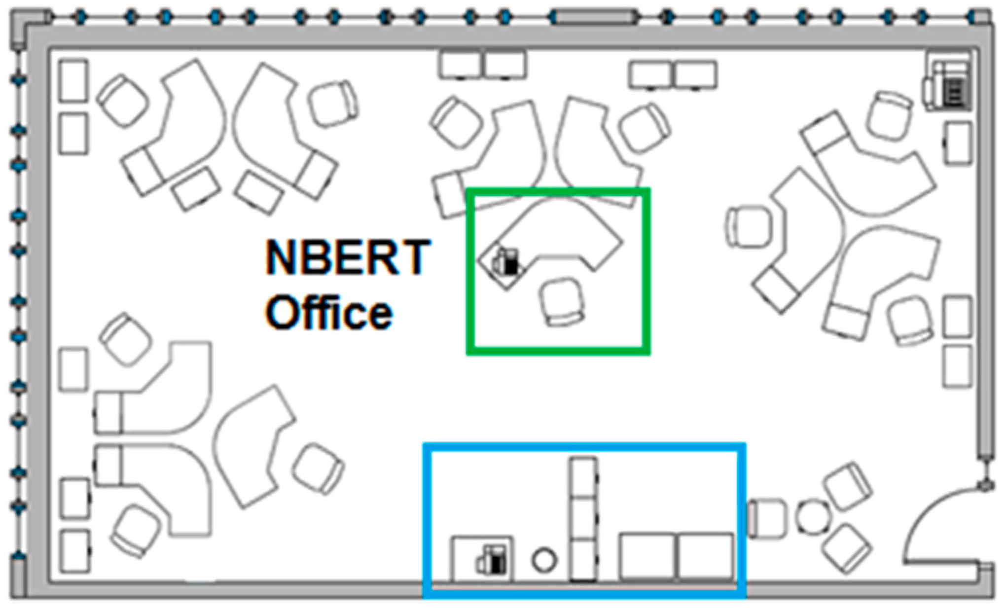
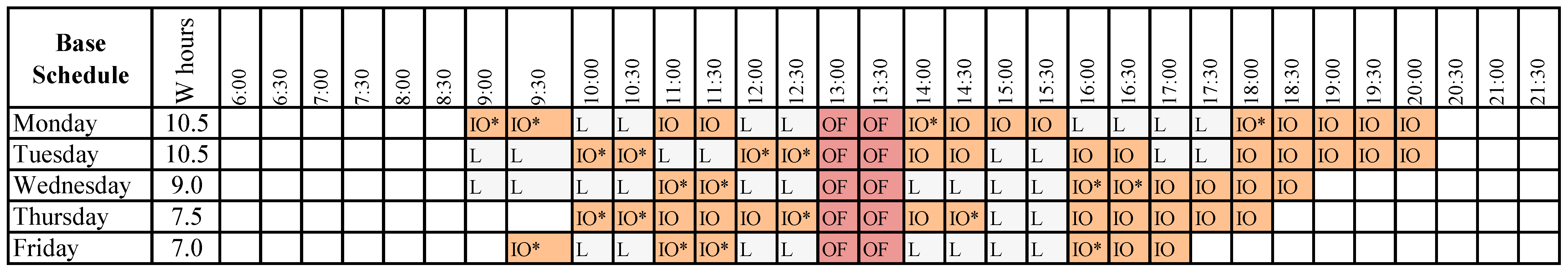
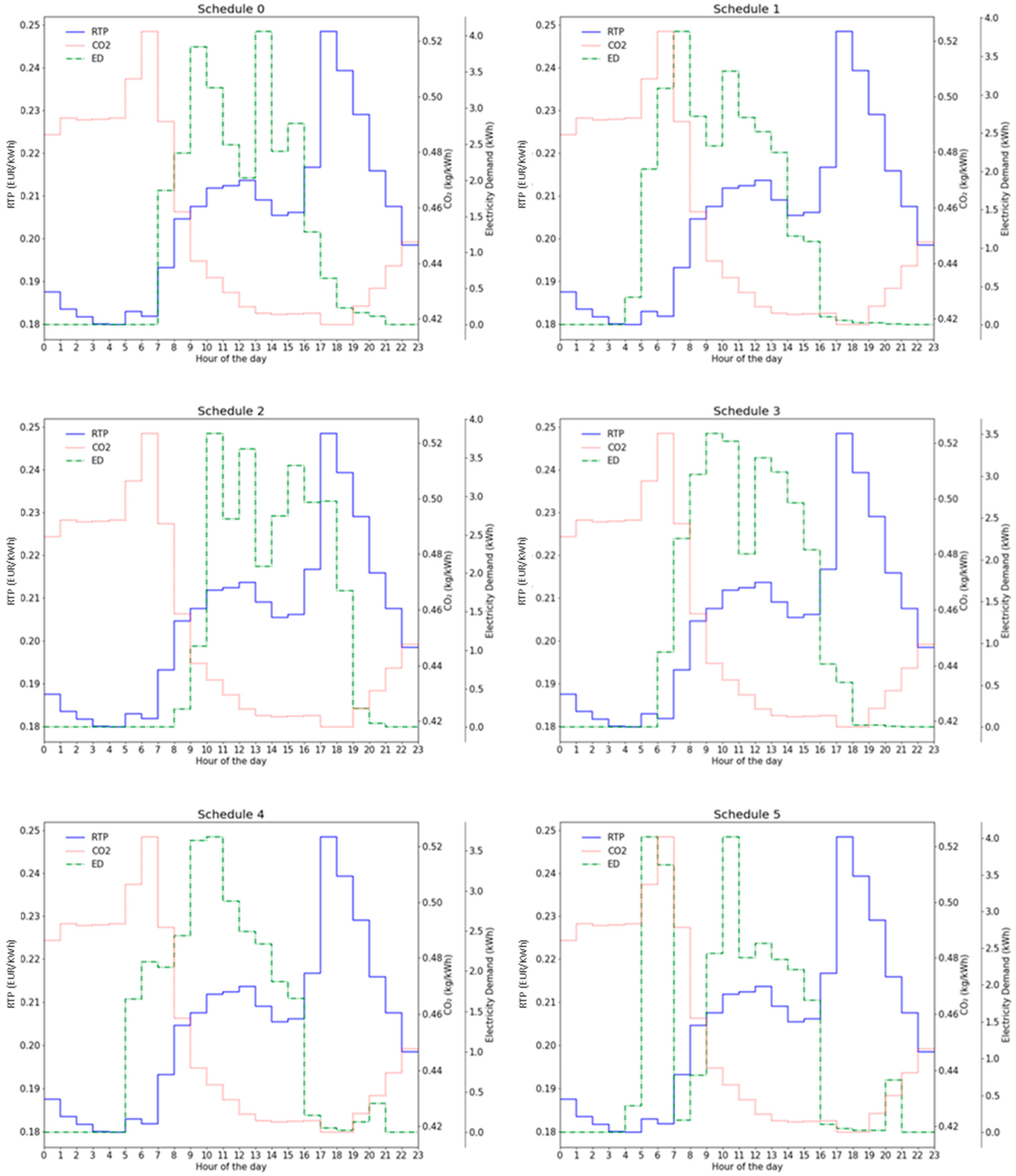
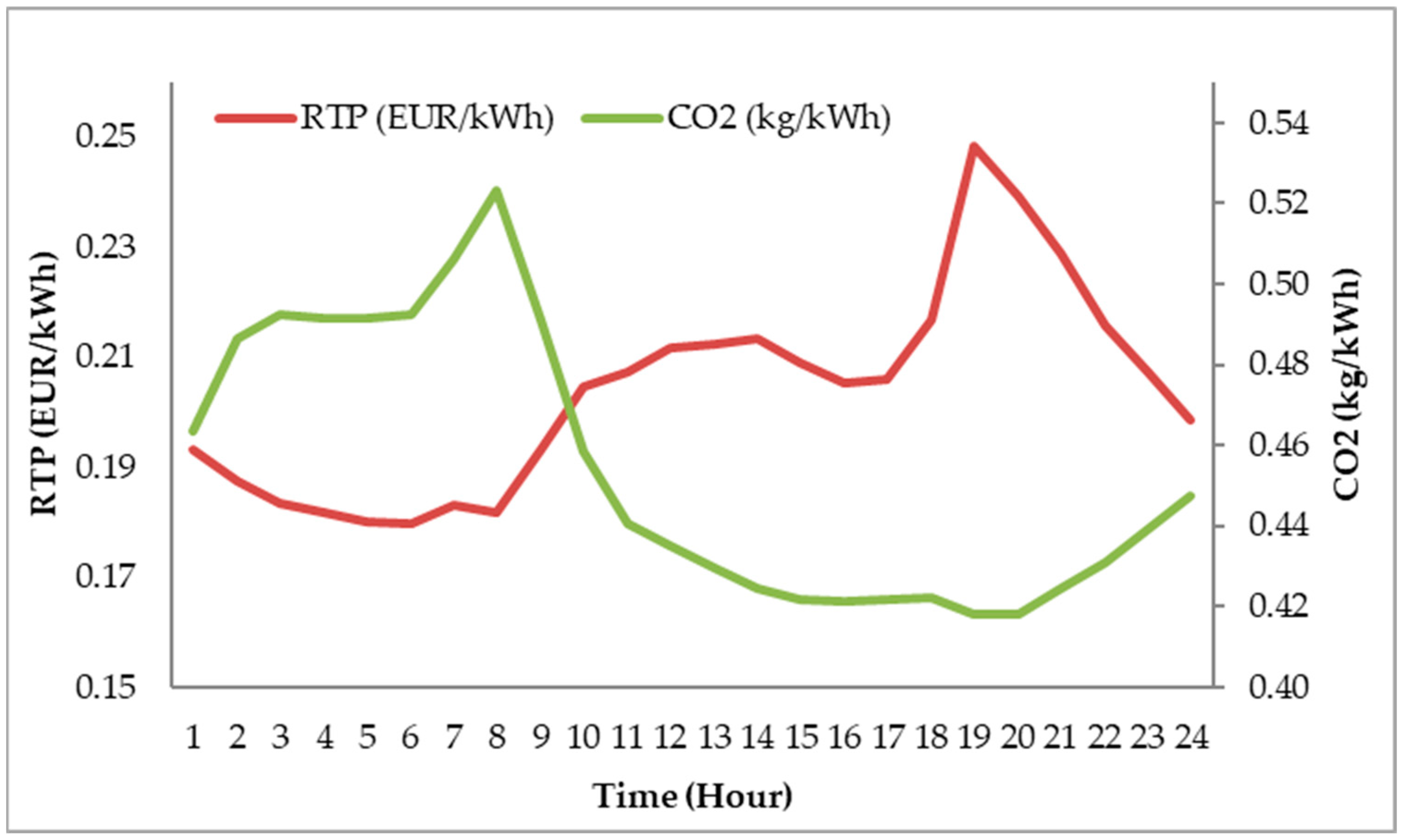
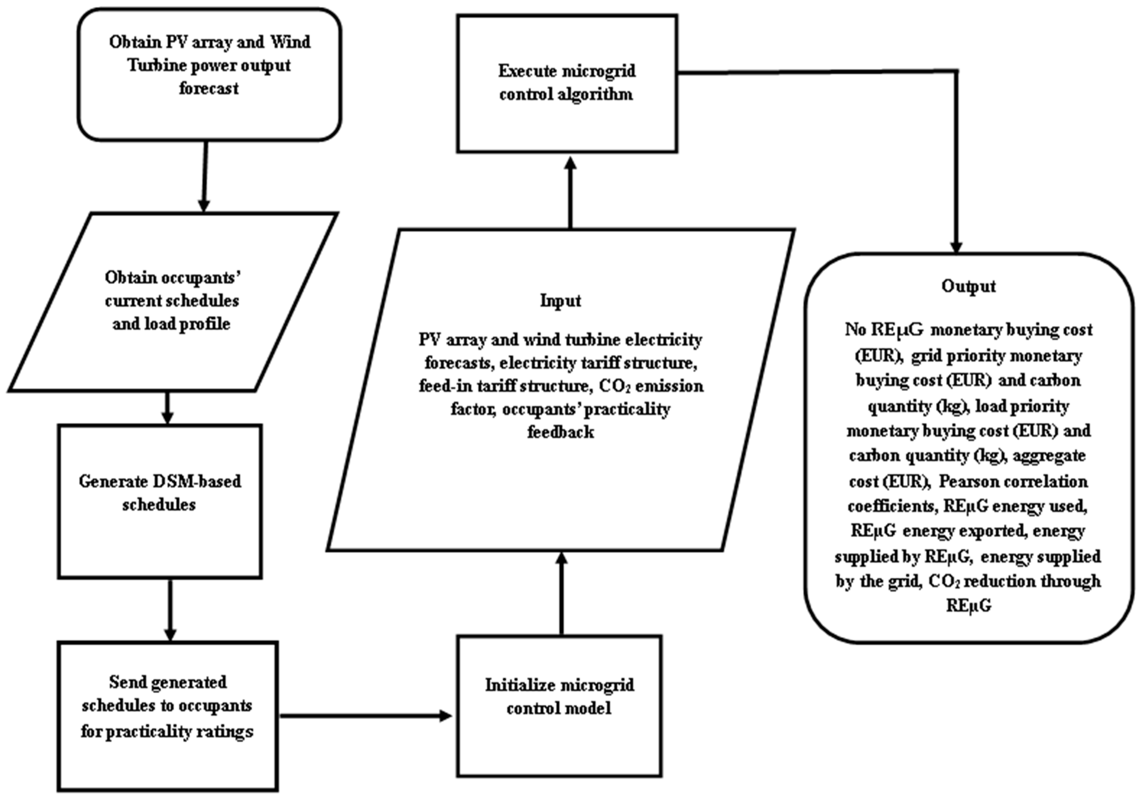
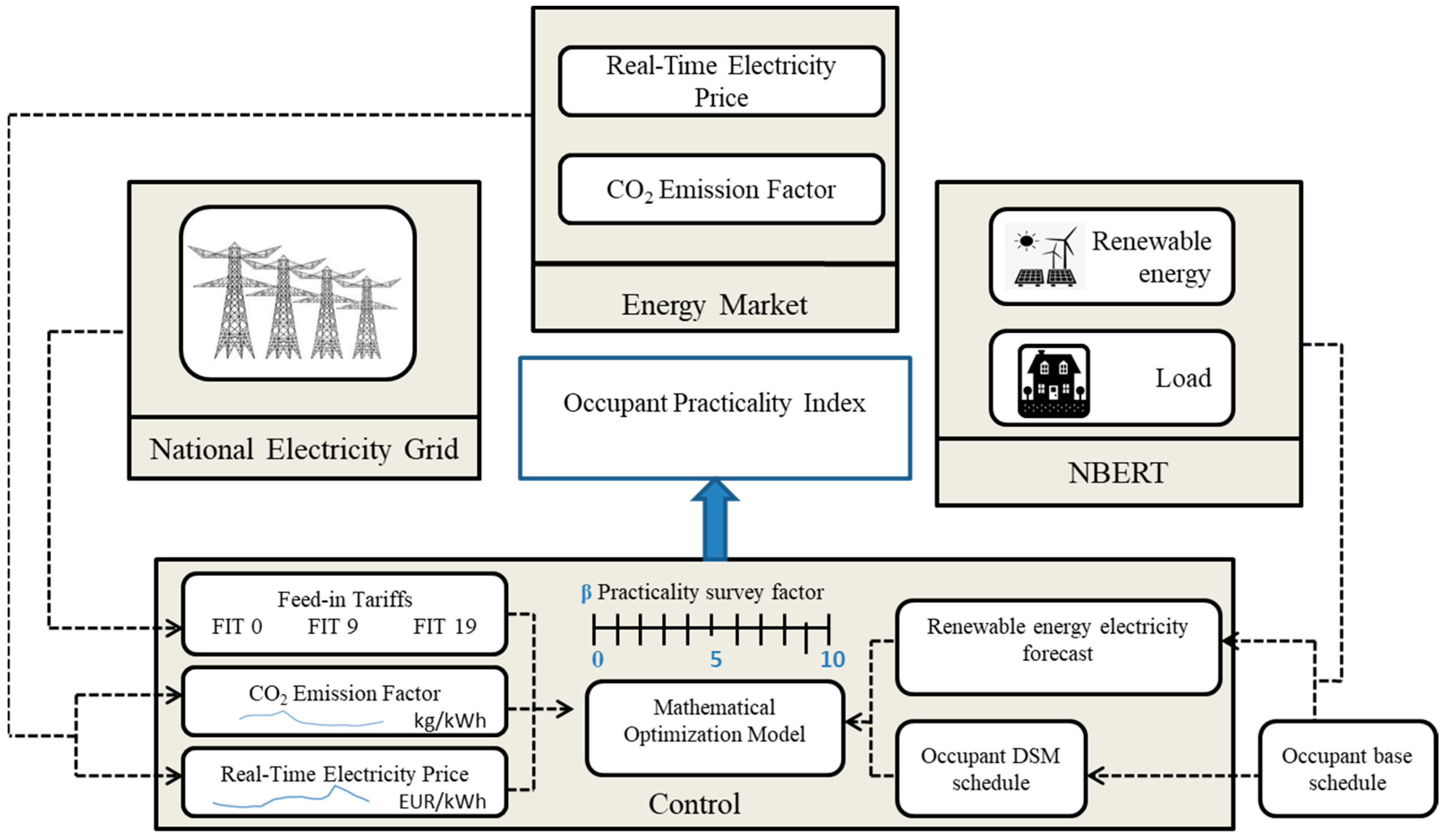
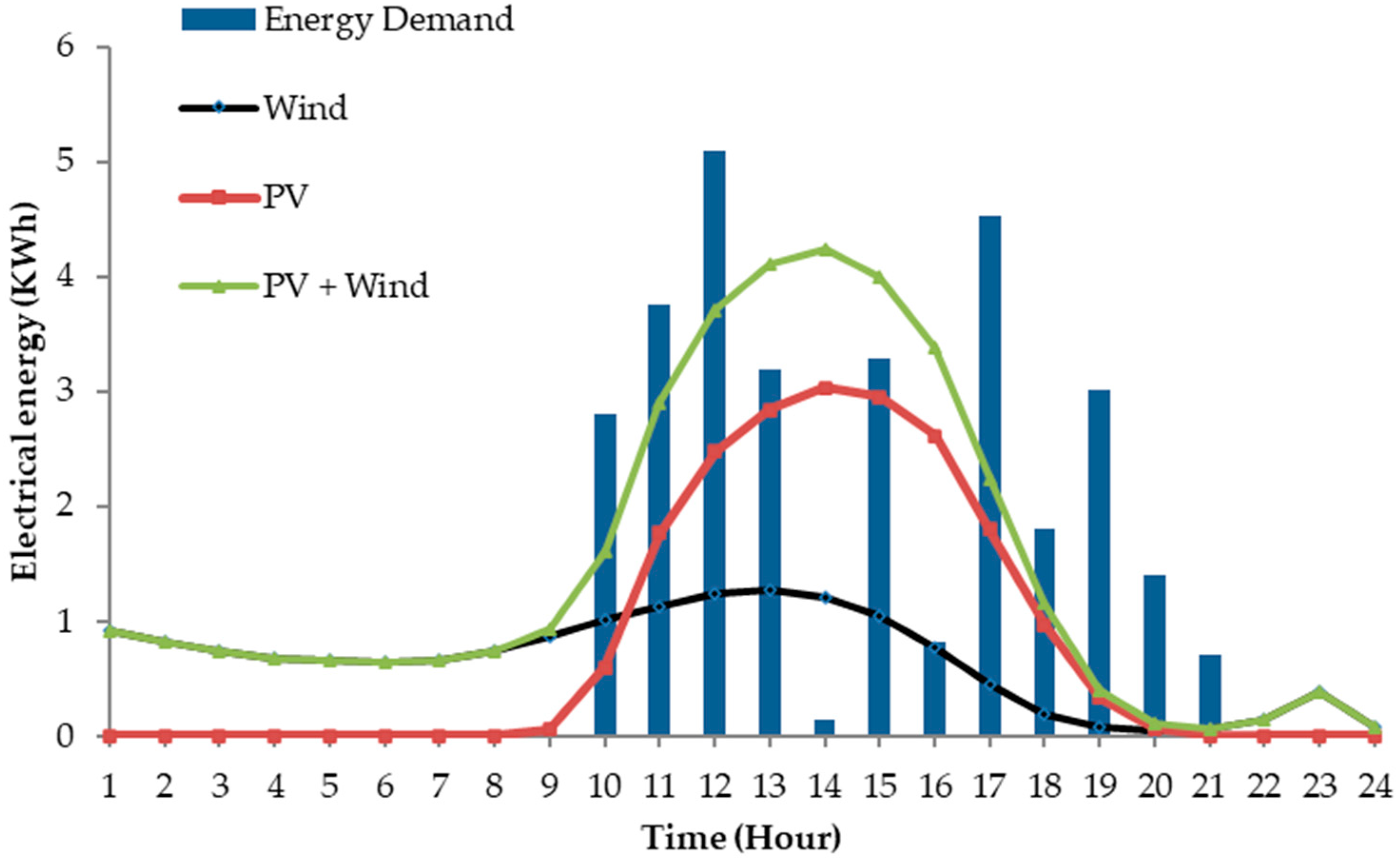
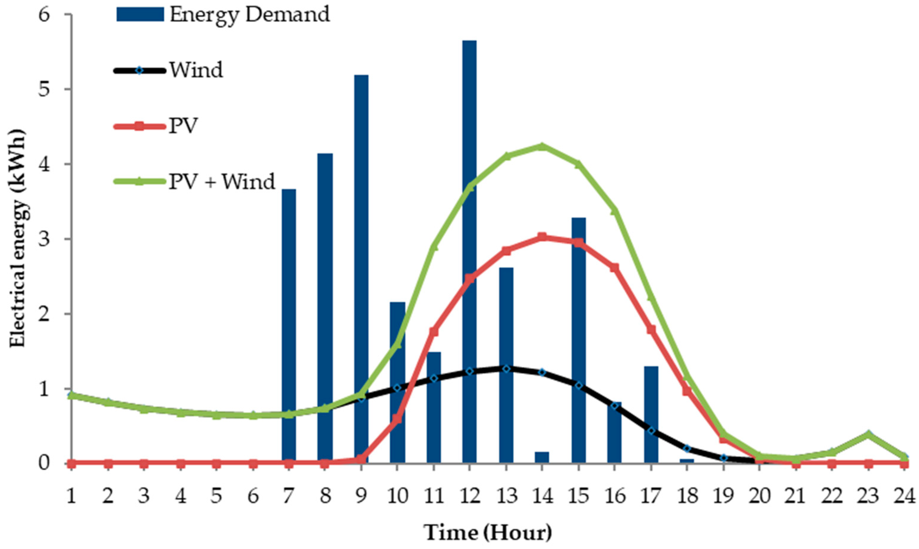
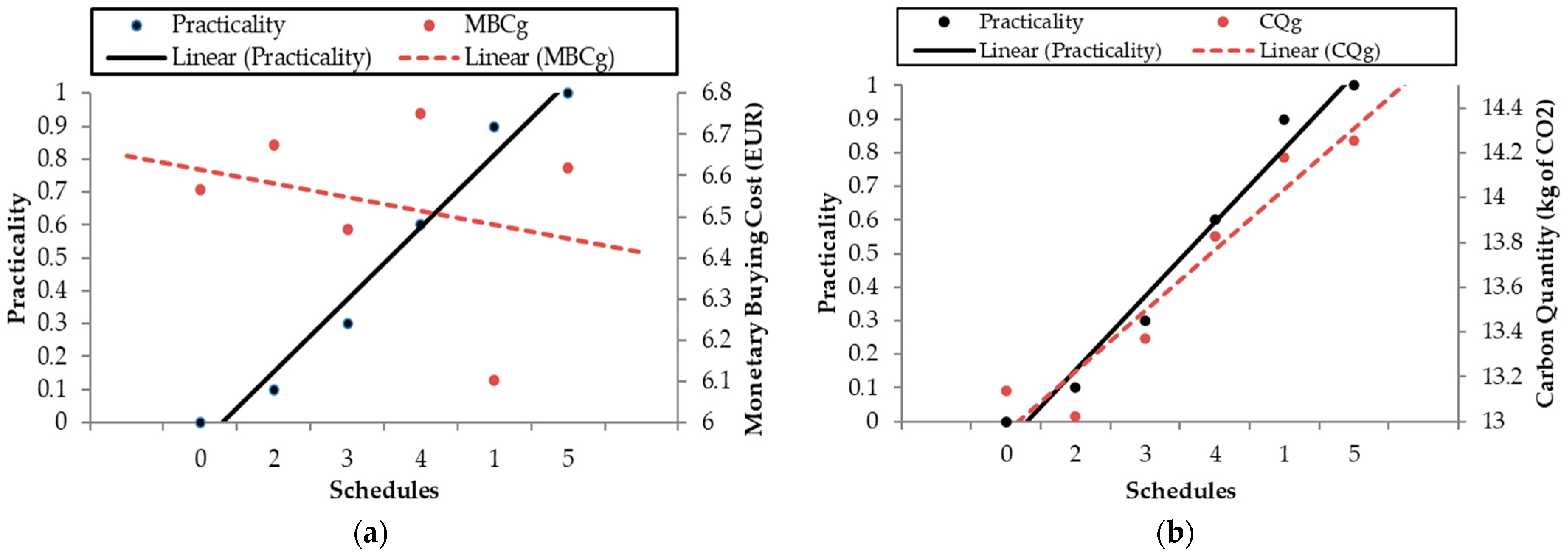
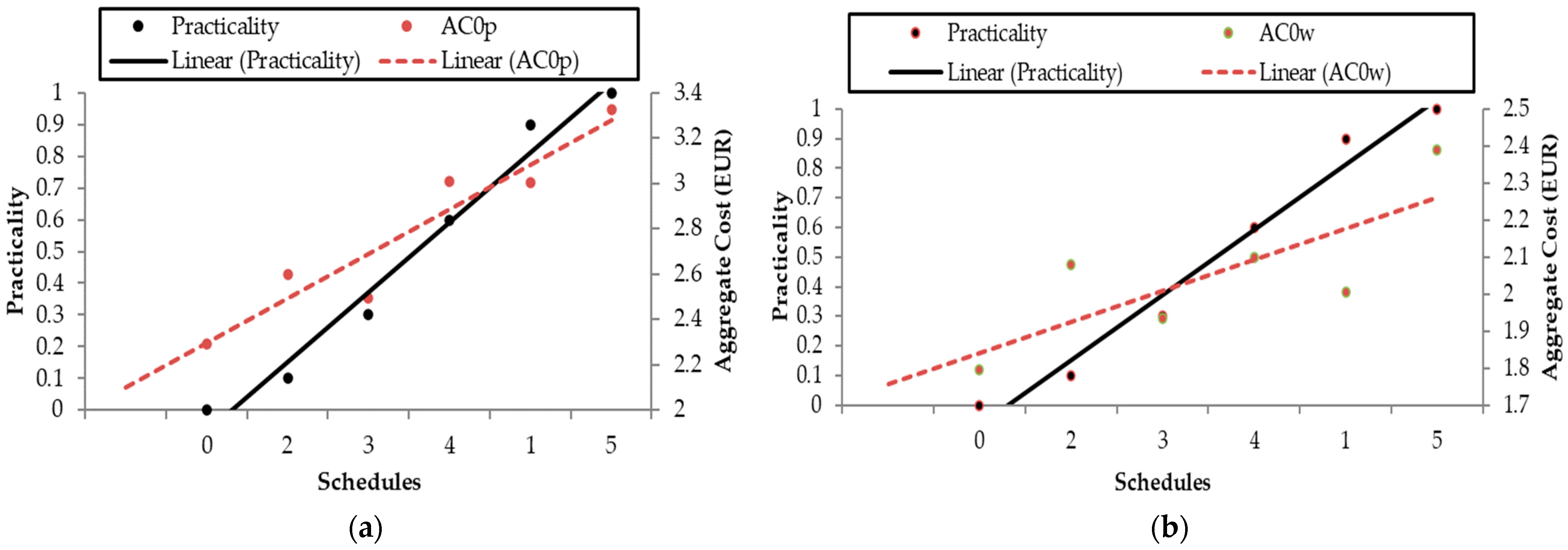
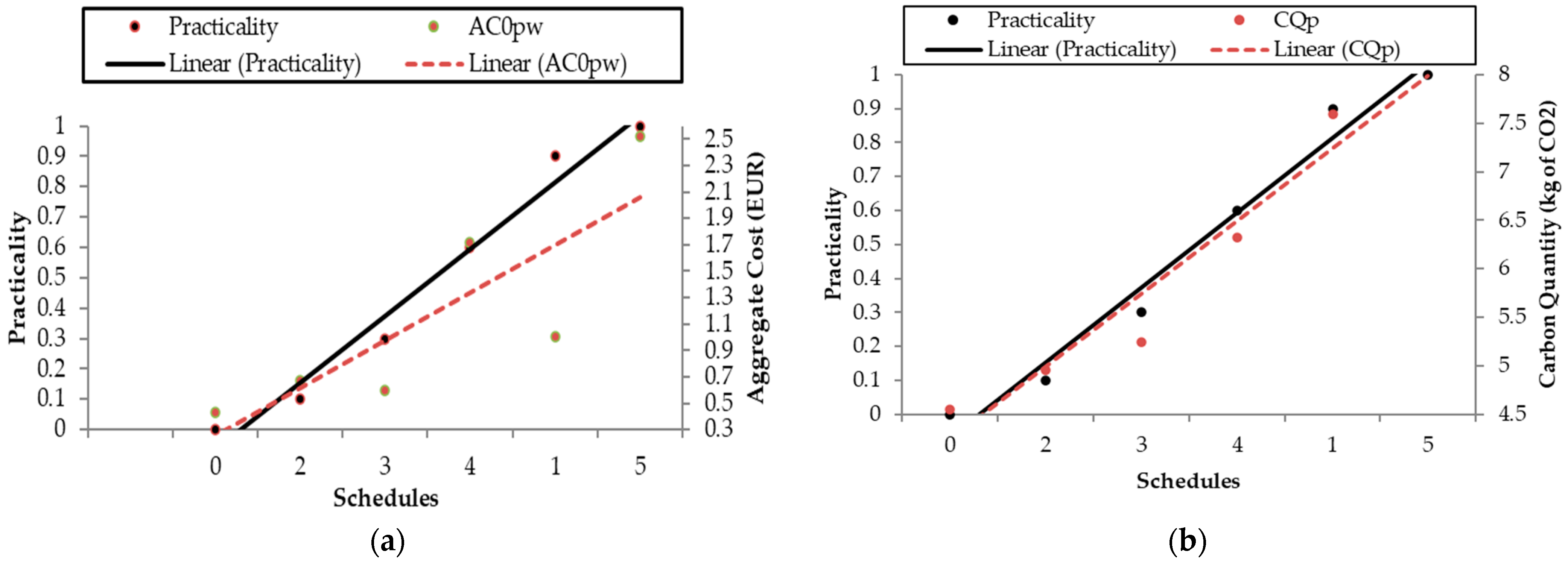
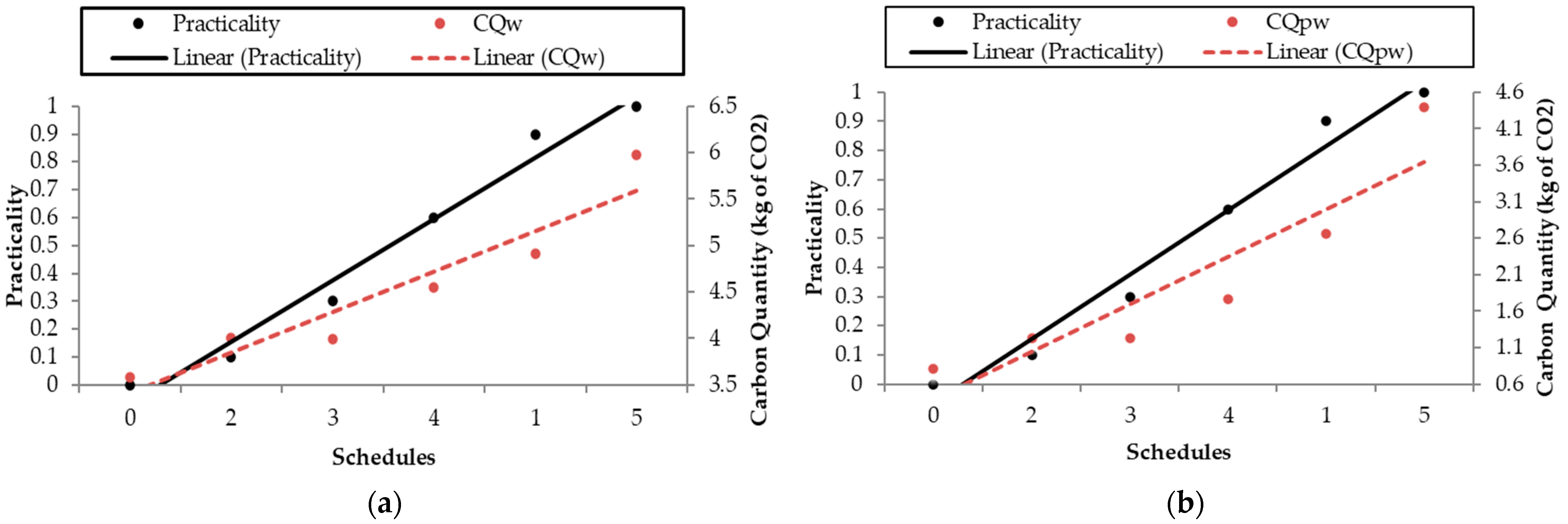
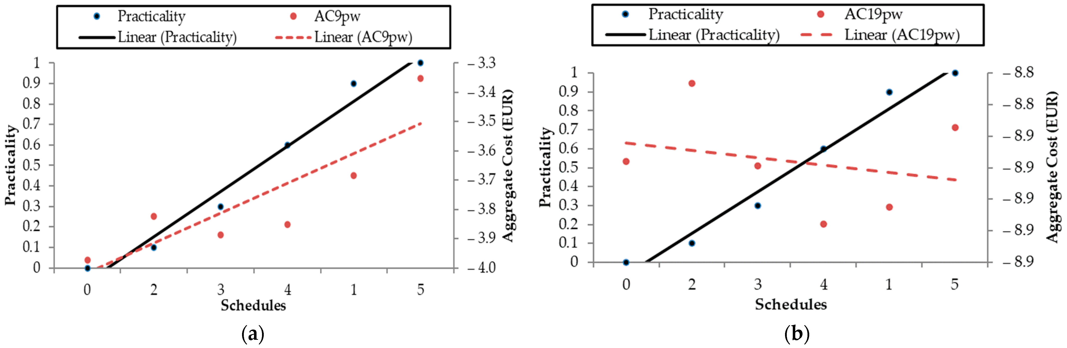
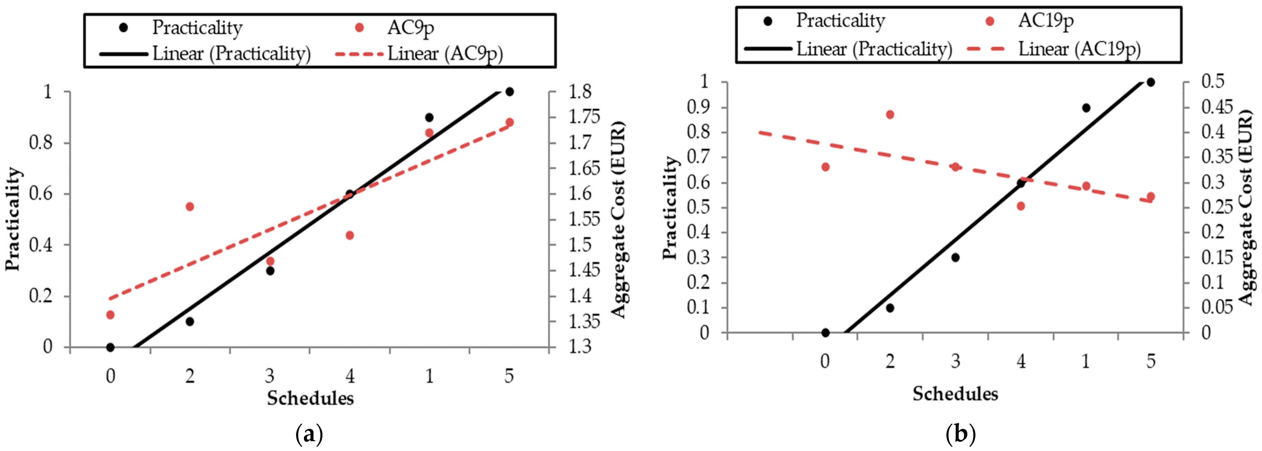

Disclaimer/Publisher’s Note: The statements, opinions and data contained in all publications are solely those of the individual author(s) and contributor(s) and not of MDPI and/or the editor(s). MDPI and/or the editor(s) disclaim responsibility for any injury to people or property resulting from any ideas, methods, instructions or products referred to in the content. |
© 2024 by the authors. Licensee MDPI, Basel, Switzerland. This article is an open access article distributed under the terms and conditions of the Creative Commons Attribution (CC BY) license (https://creativecommons.org/licenses/by/4.0/).