Atmospheric PM2.5 Prediction Model Based on Principal Component Analysis and SSA–SVM

Abstract

This paper uses an enhanced sparrow search algorithm (SSA) to optimise the support vector machine (SVM) by considering the emission of air pollution sources as the independent variable. Consequently, it establishes a PM2.5 concentration prediction model to improve the prediction accuracy of fine particulate matter PM2.5 concentration. First, the principal component analysis is applied to extract key variables affecting air quality from high-dimensional air data to train the model while removing unnecessary redundant variables. Adaptive dynamic weight factors are introduced to balance the global and local search capabilities and accelerate the convergence of the SSA. Second, the SSA–SVM prediction model is defined using the optimised SSA to continuously update the network parameters and achieve the rapid prediction of atmospheric PM2.5 concentration. The findings demonstrate that the optimised SSA–SVM prediction method can quickly predict atmospheric PM2.5 concentration, using the cyclic search method for the best solution to update the model, proving the method’s effectiveness. Compared with other methods, this approach has a small prediction error, a high prediction accuracy and better practical value.

1. Introduction

As the environmental damage intensifies, air pollution particulate matter, such as carbon monoxide (CO), carbon dioxide (CO₂), sulphur dioxide (SO₂), ozone (O₃) and particulate matter (PM2.5 and PM10), has gradually emerged as leading indicators for environmental monitoring in China [1]. Fine particulate matter (PM2.5 particulate matter) is a heavy metal pollutant that severely threatens human health and travel [2,3,4]. The possible consequences of PM2.5 pollution encompass several physiological processes, such as free radical peroxidation, disruption of intracellular calcium homeostasis, inflammatory damage and the development of cardiovascular diseases and cancer [5,6,7]. Since 2013, PM2.5 pollution has increasingly garnered public attention in China [8]. Hence, the prediction of PM2.5, a fundamental aspect of air quality management, has prompted substantial scholarly research in artificial intelligence for numerous decades [9,10].

Earlier studies [11,12,13] introduced two types of models for predicting PM2.5 concentration—deterministic models and statistical models. Deterministic models predict PM2.5 concentration by simulating the physical transport and chemical reactions of air pollutants [11,14]. Despite the advances in these methods, they are computationally expensive and unreliable for large-scale area air quality predictions due to uncertainties in photochemical diffusion mechanisms and emissions [13,15,16,17]. Statistical models, primarily referring to machine or deep learning techniques, can capture the complex relationship between PM2.5 concentration and external variables [18,19] and achieve prediction accuracy almost equivalent to that of deterministic models [20,21]. Statistical models are widely used in prediction tasks because of their incredible speed, affordability and requirement of previous knowledge [19,22,23,24,25,26]. With the breakthroughs in computing power and deep learning theories, these models can achieve better performance in PM2.5 concentration prediction tasks, paving the way for extensive applications of statistical models in atmospheric environmental science [18,19].

The formation of PM2.5 is affected by several factors, such as humidity, wind speed, temperature, rainfall and others. Therefore, this complexity causes the forecasting model to deal with high-latitude data, which are often redundant, in predicting PM2.5 concentrations, making it necessary to extract effective variables for accurate predictions. Many scholars have conducted numerous studies on pollution issues to monitor and predict air pollution in recent years. Existing research demonstrates that models based on machine learning and deep learning, such as multilayer perceptron models [27], the backpropagation neural network (BPNN) model [28], support vector regression (SVR) [29,30], the random forest (RF) model [30,31,32], the general regression neural network model [28,33,34] and the recursion neural network model [35], have been successfully used in atmospheric environment modelling for monitoring and predicting atmospheric pollutants. Wu et al. [36] used an enhanced neural network prediction model to predict PM10 air indicators in urban Wuhan and revealed that the improved neural network model has a higher prediction accuracy. The RF and k-nearest neighbour (KNN) algorithms were used [37,38] to further improve the pollutant prediction efficiency. These methods decreased the response time of gas prediction to some degree. Nevertheless, with the expansion of the training sample count, KNN experienced an escalated computational burden and developed a diminished capacity to tolerate errors in the training data with a tendency to overfit during classification [39] due to its sensitivity to minor changes in the training dataset.

The support vector machine (SVM) is commonly employed to address regression and classification tasks [40]. Compared to other classifiers, like RF and Bayesian, this particular classifier demonstrates notable advantages in addressing challenges related to limited sample size, non-linear relationships and high-dimensional data. Despite these advantages, it maintains high accuracy and efficiency [41]. Nevertheless, the choice of parameters considerably influences the SVM’s prediction performance. In real-world scenarios, determining parameters often relies on empirical methods or trial algorithms. Consequently, the resulting prediction accuracy tends to fall short of the desired goal accuracy because of the incorrect selection of parameters. Expanding the search space to identify the globally optimal solution will reduce the efficiency of the model’s forecast time. Various optimisation methods, including the genetic algorithm (GA) [42,43], particle swarm optimisation (PSO) algorithm [44,45], ant colony algorithm [46] and cetacean optimisation algorithm [47], have been forwarded as potential approaches to address the SVM parameter problem.

In 2020, Xue introduced the sparrow search algorithm (SSA) [48]. The SSA model primarily aims to replicate the foraging and anti-predation behaviours exhibited by sparrows. Compared to existing swarm intelligence optimisation algorithms, this approach has superior optimisation capability, rapid convergence rate and favourable stability. In addition, it demonstrates significant robustness [49]. SSA is beneficial in locating the global optimal prospective area and mitigating the occurrence of the local optimal dilemma due to its exceptional search capability. However, SSA-optimised SVMs have some shortcomings: insufficient diversity of the initial population can lead to poor convergence ability of the algorithm in subsequent iterations [50] and insufficient search accuracy due to the high convergence operator speed of the method.

To address the large redundancies in air pollutant data, low accuracy of air pollutant prediction and the shortcomings in the SSA–SVM model, a PM2.5 concentration prediction method based on SSA–SVM was proposed in this study. Its contributions are summarised below.

(1)

Principal component analysis (PCA) is combined with SSA–SVM to reduce the redundancy of air pollution data and analyse air pollution data. Next, an SVM hyperparameter optimisation algorithm is designed based on the SSA.

(2)

The SVM parameter selection is solved using the SSA algorithm. For the SSA, a spread that can change the adjustable operator, ω, is added to enhance the SSA. Next, the improved sparrow search method determines the best SVM parameters. The refined SSA-SVR is better at predicting the amount of pollution in the air. How well does the guess about the gas concentration fit? The prediction results demonstrate how well the proposed model worked at predicting PM2.5 concentrations and improving SVM parameters, confirming its reliability and suitability.

2. Study Area and Data

Jilin Province is a major grain-producing province in China, and air pollution has considerably affected its agricultural output. Since 2013, China has set up numerous air quality monitoring stations, but the Jilin region still lacks air pollution management practices. Therefore, the historical data of PM10, PM2.5, SO₂, NO₂, CO, O₃, temperature and humidity collected between October and December 2020 were selected as the research objects to evaluate the accuracy of the proposed method in predicting PM2.5 concentration. This study collected hourly historical PM2.5 concentrations from 30 air quality monitoring stations in the Jilin Province from 1 January 2019 to 31 December 2022. PM2.5 concentration data were obtained from the national urban air quality real-time platform (http://www.weather.com.cn/ (accessed on 1 August 2023)) and meteorological data service centre (http://data.cma.cn/en (accessed on 1 August 2023)). The adjacent short-term values interpolate the missing PM2.5 concentration data to verify the proposed model’s performance. Figure 1 depicts the study areas and locations of 30 air quality monitoring stations in the Jilin Province.

3. Materials and Methods

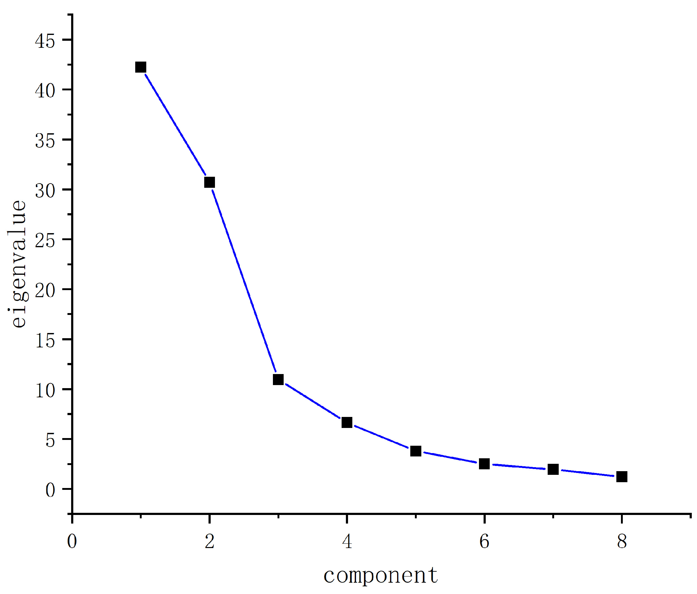
3.1. Principal Component Analysis

Because several factors affect atmospheric changes in the air pollution monitoring process, this paper adopts the PCA method to extract the collected variables as follows. First, the collected pollution gases, namely PM10, PM2.5, NO₂, SO₂ and O₃, and the time series of meteorological conditions (temperature and humidity) are taken as samples. The observed data matrix is shown as follows:

$$X=\left(\begin{array}{cccc}{\mathrm{x}}_{11}& {\mathrm{x}}_{12}& \dots & {\mathrm{x}}_{1\mathrm{p}}\\ {\mathrm{x}}_{21}& {\mathrm{x}}_{22}& \dots & {\mathrm{x}}_{2\mathrm{p}}\\ ⋮& ⋮& ⋮& ⋮\\ {\mathrm{x}}_{\mathrm{n}1}& {\mathrm{x}}_{\mathrm{n}2}& \dots & {\mathrm{x}}_{\mathrm{np}}\end{array}\right)$$

(1)

where n is the number of monitored samples; p is the monitored indicator; and x₁₁, x₁₂, …, x_n1 are the time series of PM10, PM2.5, NO₂, SO₂, O₃ and meteorological conditions (temperature and humidity) in the sample data. Because of inconsistency in the dimensions of different collected samples, it is necessary to standardise the collected data and calculate the standardised correlation coefficient matrix.

The calculation formula is defined as follows:

$${\mathrm{r}}_{\mathrm{ij}}=\frac{{\displaystyle \sum _{k=1}^n\left(x_{ki}-\overline{x_i}\right)\left(x_{kj}-\overline{x_j}\right)}}{\sqrt{{\displaystyle \sum _{k=1}^n{\left(x_{ki}-\overline{x_i}\right)}^2{\displaystyle \sum _{k=1}^n{\left(x_{kj}-\overline{x_j}\right)}^2}}}}$$

(2)

In the above formula, the variable represents the mean value of row i in the X matrix. The outcome of this computation presents a correlation coefficient matrix.

We then found the eigenvalues (λ₁, λ_2, …, λ_p) and the corresponding eigenvectors (α_j1, α_j2, …, α_jp) of the R matrix. Its principal component expression is as follows:

$$Z_{\mathrm{i}}={\mathrm{a}}_{\mathrm{j}1}{X}_1+{\mathrm{a}}_{\mathrm{j}2}{X}_2+\dots {\mathrm{a}}_{\mathrm{jp}}{X}_{\mathrm{p}}$$

(3)

where Z_i represents the p-th principal component, whereas X₁–X_p correspond to the variables x_i1–x_ip. Subsequently, it is possible to ascertain the variables that significantly influence pollution by calculating the contribution and cumulative contribution rates of the primary components. The formula is expressed as follows:

$$C_{\mathrm{r}}={\lambda }_{\mathrm{i}}/{\displaystyle \sum _{\mathrm{i}=1}^{\mathrm{p}}{\lambda }_{\mathrm{i}}}$$

(4)

where C_r is the contribution rate. The cumulative contribution rate ranges from 85% to 95%, which is determined by the corresponding number of principal components. Next, the influencing factors of the collected data are calculated, and the number of principal components is determined from the cumulative contribution rate (

Table 1. Principal component contribution rate.

Variable	Number	Eigenvalue	Contribution Rate	Accumulated Contribution Rate
PM2.5	1	42.236	42.236	42.236
PM10	2	30.720	30.720	72.956
SO2	3	10.945	10.945	83.901
NO2	4	6.633	6.632	90.533
NO	5	3.797	3.798	94.331
O3	6	2.502	2.501	96.832
Temperature	7	1.947	1.947	98.779
Relative humidity	8	1.221	1.221	100.000

).

Figure 2 shows that the first factor’s eigenvalue (variance contribution) is very high. Moreover, it makes the highest contribution to the solution of the total interpretation data. The fourth factor, after the eigenvalues, is small. The contribution to the interpretation of the principal component is small and can be ignored; therefore, it is more appropriate to extract four factors.

The component matrix presents the correlation between the four principal components, and x1 ~ 4 are determined as principal component variables. The PM2.5 concentration is one of the primary components causing pollution. Therefore, this paper mainly conducts prediction research on predicting PM2.5 levels. The component matrix results show that the PM2.5 concentration is closely related to the other four variables. The PM2.5 concentration will also increase accordingly with the increase in PM10. However, the PM2.5 concentrations decrease accordingly with the increase in the concentrations of SO₂ and O₃.

Table 2. Principal component analysis factor matrix.

Variable	X1	X2	X3	X4
PM2.5	0.876	0.294	0.059	−0.135
PM10	0.908	−0.121	0.103	–0.003
SO2	0.121	0.848	0.037	0.871
NO2	0.600	0.560	−0.435	−0.053
NO	0.634	0.146	−0.042	−0.025
O3	0.499	−0.547	0.763	0.342
Temperature	0.534	−0.749	−0.128	−0.150
Relative humidity	0.074	0.665	0.611	0.382

shows that the extracted main components are related to the PM2.5 concentration and affect the PM2.5 concentration.

The factor analysis is a multi-statistical method based on the study of internal dependencies among various variables, and it classifies some variable indicators with overlapping information and high correlations into several uncorrelated comprehensive factors. The table shows that PM2.5 and PM10 exert a higher load on the first factor, which can explain these items. SO₂ has a higher load on the second factor, O₃ has a higher load on the third factor and SO₂ has a higher load on the fourth factor. Therefore, this paper finally selected PM10, PM2.5, SO₂ and O₃ as the primary vital variables and determined them as the input variables of the established PM2.5 prediction model.

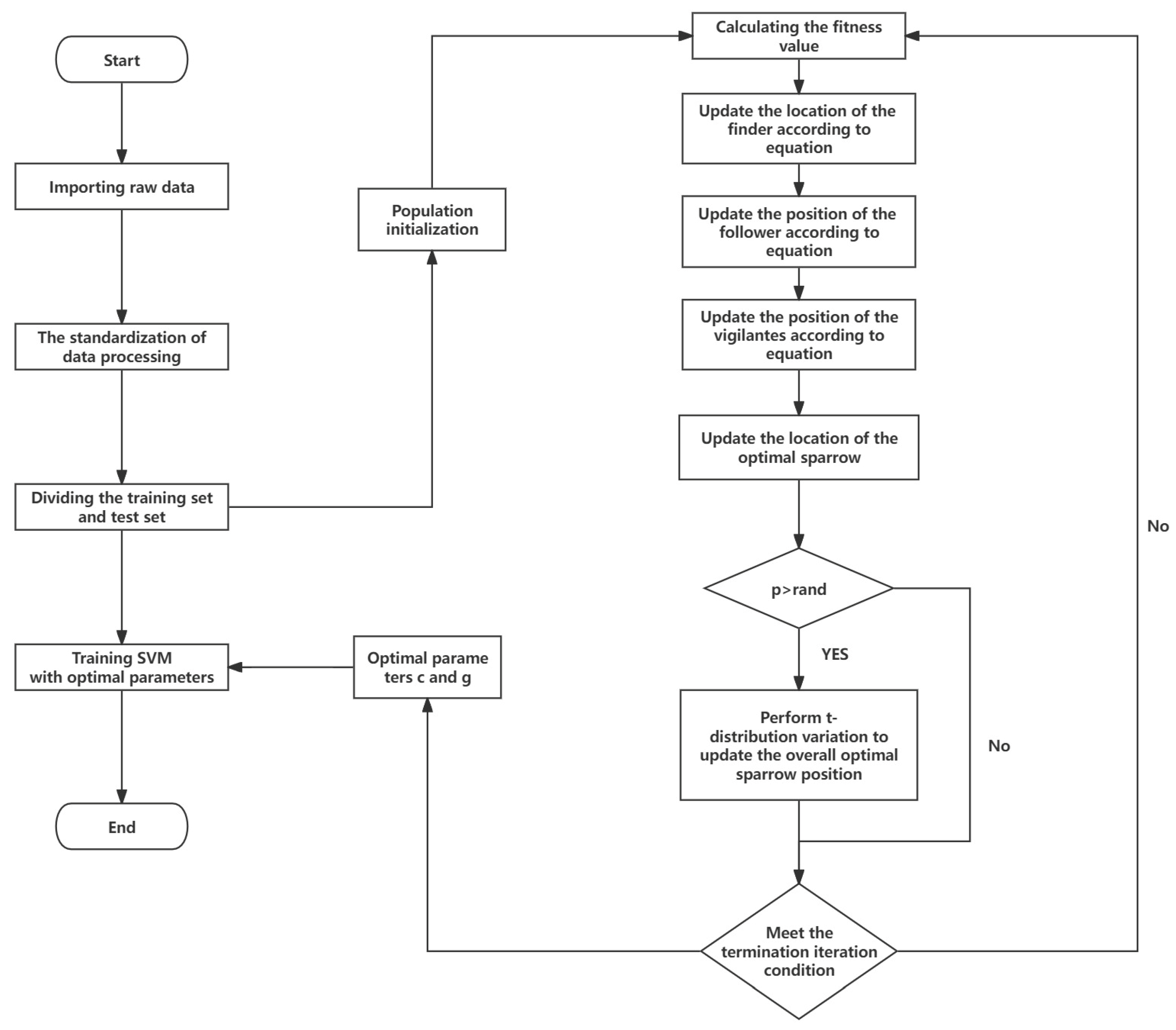
3.2. Building SSA–SVM Prediction Model

3.2.1. Sparrow Search Algorithm

SSA is a new swarm intelligence algorithm [50,51] that was created after drawing inspiration from the sparrow’s three behaviours of predation, following and detection. The algorithm divides the sparrow population into the finder and the follower. The sparrow’s property is the location corresponding to the optimised solution, and the fitness value corresponds to the foraging location. The location of the finder and the follower is dynamically changing, and the finder will select the best location to forage. The follower will forage around the finder or compete with the finder for food and update the finder’s solution when the follower finds a better location for food; otherwise, it will stay unchanged. When a danger is detected, the marginal sparrows migrate to the safe zone to avoid it, whereas those in the best position move around. The SSA searches for the optimal solution based on the above steps.

Suppose a sparrow population consists of n sparrows, and the parameter dimension that needs to be optimised is m. The population can be expressed as follows:

$$X=\left(\begin{array}{cccc}{\mathrm{x}}_{1,1}& {\mathrm{x}}_{1,2}& \dots & {\mathrm{x}}_{1\mathrm{m}}\\ {\mathrm{x}}_{2,1}& {\mathrm{x}}_{2,2}& \dots & {\mathrm{x}}_{2,\mathrm{m}}\\ ⋮& ⋮& ⋮& ⋮\\ {\mathrm{x}}_{\mathrm{n},1}& {\mathrm{x}}_{\mathrm{n},2}& \dots & {\mathrm{x}}_{\mathrm{n},\mathrm{m}}\end{array}\right)$$

(5)

The fitness value, F(x), of all sparrows is expressed as follows:

$$F_X=\left[\begin{array}{c}f\left(\left[\begin{array}{cccc}{x}_{1,1}& x_{1,2}& \cdots & x_{1,m}\end{array}\right]\right)\\ f\left(\left[\begin{array}{cccc}{x}_{2,1}& x_{2,2}& \cdots & x_{2,m}\end{array}\right]\right)\\ ⋮\\ f\left(\left[\begin{array}{cccc}{x}_{n,1}& x_{n,2}& \cdots & x_{n,m}\end{array}\right]\right)\end{array}\right]$$

(6)

The finder is responsible for finding food for the group; hence, it has a more extensive food search area. In each iteration, the discoverer’s position is updated as follows:

$$X_{ij,t+1}=\left\{\begin{array}{c}{X}_{ij.t}\cdot \exp \left(\frac{-i}{\alpha ite{r}_{\max }}\right),R_2<ST\\ X_{i,j}^{\mathrm{t}+1}+QL\end{array}\right.$$

(7)

The formula has three variables: t, which stands for the current iteration number; αiter_max stands for the maximum number of iterations; X_ij represents the position information of the i-th sparrow in the j-th parameter dimension; α ∈ [0, 1] is a random number, R₂ ∈ [0, 1] represents the alarm value; ST ∈ [0.5, 1] represents the safety value; Q is a random number obeying the normal distribution; and all element values in the matrix are 1.

The follower position is updated as follows:

$$X_{ij,t+1}=\left\{\begin{array}{c}Q\exp \left(\frac{x_{worst}^t-x_{i,j}^t}{\alpha ite{r}_{\max }}\right),i<\frac{n}{2}\\ X_p^{\mathrm{t}+1}+\left|x_{i,j}^t-X_p^{t+1}\right|A^{+}L\end{array}\right.$$

(8)

A⁺ = A^T (AA^T) − 1, where A is a matrix of size 1 × D, and x_worst is the worst position. When i > n/2, its value will converge to 0, and the i-th sparrow with less food needs to update its position to obtain food. When i ≤ n/2, the i-th sparrow is near the best foraging position, and its value converges to the optimal position.

The scout position is described as follows, generally accounting for 10–20% of the total number of sparrows:

$$X_{i,j}^{\mathrm{t}+1}=\left\{\begin{array}{c}{x}_{best}^t+\beta \left|x_{i,j}^t-x_{best}^t\right|,f_i>f_g\\ X_{i,j}^{\mathrm{t}}+K\left(\frac{\left|x_{i,j}^t-x_{worst}^t\right|}{f_i-f_w+\epsilon }\right),f_i=f_g\end{array}\right.$$

(9)

where f_i is the current sparrow individual’s fitness value; f_g is the sparrow’s best position at the global ideal location; x_best is the optimal position; and β is a random number that follows the normal distribution, with a mean of 0 and a variance of 1. The optimal fitness value is represented by fw, which is the sparrow’s fitness value at its worst location; K is a random value within the interval [−1, 1] and ε is a minimal number that keeps the denominator from zero.

3.2.2. Improved Sparrow Search Algorithm

Insufficient search occurs due to a decrease in the SSA’s population diversity, as shown by the exponential function in an equation, indicating a slightly faster decline speed and smaller disturbance range at the start of the iteration. Furthermore, the method has a sluggish decay rate, and a wider range of disturbances in the later stages will hinder convergence. A dynamic adaptive weight improvement optimisation technique is developed to increase the algorithm’s search optimisation capabilities and convergence speed [52].

The system’s search capabilities alter with the number of iterations because of the adaptive dynamic weight, which may effectively regulate the balance between the global search and local search of the algorithm. Earlier in the search process, when a more extensive search area is needed, more weight must be assigned to each sparrow to increase the population’s capacity to look over a wider area.

This study incorporates dynamic adaptive weights into the formula for updating producer locations to enhance the algorithm’s search performance. The mathematical representation of the variable ω can be expressed as follows:

$$\left\{\begin{array}{c}a\left(t\right)=\exp \left(2\cdot \frac{1-\sin \left(\pi t\right)}{ite{r}_{\max }}\right)-\exp \left(2\cdot \frac{1-\sin \left(\pi t\right)}{ite{r}_{\max }}\right)+\alpha \\ b\left(t\right)=\exp \left(2\cdot \frac{1-\cos \left(\pi t\right)}{ite{r}_{\max }}\right)-\exp \left(2\cdot \frac{1-\cos \left(\pi t\right)}{ite{r}_{\max }}\right)+\beta \\ \omega \left(t\right)=\frac{a\left(t\right)}{b\left(t\right)}\end{array}\right.$$

(10)

The variable “iter_max” denotes the maximum number of iterations for the method, whereas “α” and “β” are random values that fall inside the interval [0, 1]. The graph depicts the relationship between the variable ω and its corresponding function. After including the variable ω, the modified equation for the producer position is defined as follows:

$$X_{i,j}^{\mathrm{t}+1}=\left\{\begin{array}{c}\left(X_{i,j}^{\mathrm{t}}+\omega \cdot \left(f_{ib}^t-X_{i,j}^t\right)\right)\cdot \alpha R_2<ST\\ \omega \cdot X_{i,j}^{\mathrm{t}+1}+QL\end{array}\right.$$

(11)

In addition, the primary process of building the model is shown in Figure 3.

Because there are several influencing factors of PM2.5 and there is a strong correlation between the influencing factors, this paper first introduces the PCA for feature selection. It chooses the optimal feature subset as the input of the SVM model. At the same time, considering that the changes in PM2.5 concentration are difficult to predict by the traditional SVM model, the improved SSA was introduced to improve the traditional SVM model. Finally, a hybrid model was constructed.

4. Results

The experimental design involved designating the initial 80% of the data as the training set, whereas the remaining data were utilised as the test set. The algorithm code presented in this article is executed on a 24 G memory computer powered by an Intel (R) Core (TM) [email protected] GHz–2.59 GHz. To mitigate the impact of varying magnitudes and dimensions, the input data of the gathered samples underwent normalisation throughout the data processing phase. The formula for the same is expressed below:

$$x_p=\frac{x_i-x_{\min }}{x_{\max }-x_{\min }}$$

(12)

where x_p represents the normalised sample data; x_i represents the original data input; and x_max and x_min reflect the maximum and minimum values within the original data set, respectively. Figure 3 depicts the time series of the measured real PM2.5 concentration.

4.1. Evaluation Index

This research evaluates the model’s prediction accuracy by citing three statistics: mean absolute error (MAE), root mean square error (RMSE) and the coefficient of determination (R²). These statistical parameters are expressed as follows:

$$MAE=\frac{1}{\mathrm{n}}{\displaystyle \sum _{i=1}^n\left|Y_i-Y_i^{\ast }\right|}$$

(13)

$$RMSE=\sqrt{\frac{1}{n}{\displaystyle \sum _{i=1}^n{\left(Y_i-Y_i^{\ast }\right)}^2}}$$

(14)

$$R^2=1-\frac{{\displaystyle \sum _{i=1}^n{\left(Y_i-Y_i^{\ast }\right)}^2}}{{\displaystyle \sum _{i=1}^n{\left(Y_i-\overline{Y_i}\right)}^2}}$$

(15)

where n is the number of test set samples; and Y_i and Y_i* are the measured and anticipated values of PM2.5 concentration, respectively. The four indications listed above are used to assess the trial outcomes. The better the prediction outcome, the lower the values of the first two indicators. The opposite is true for the R² value. The quality of the experimental outcome increases with value.

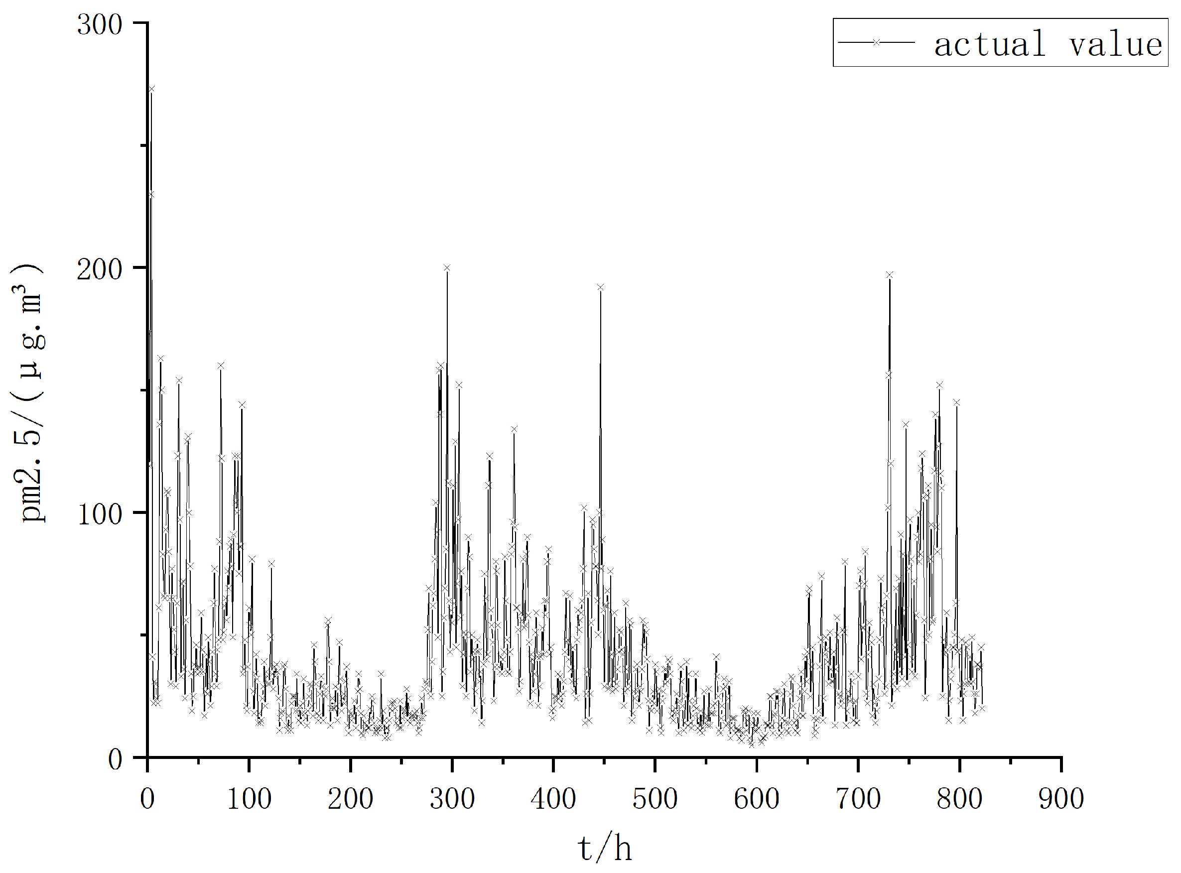
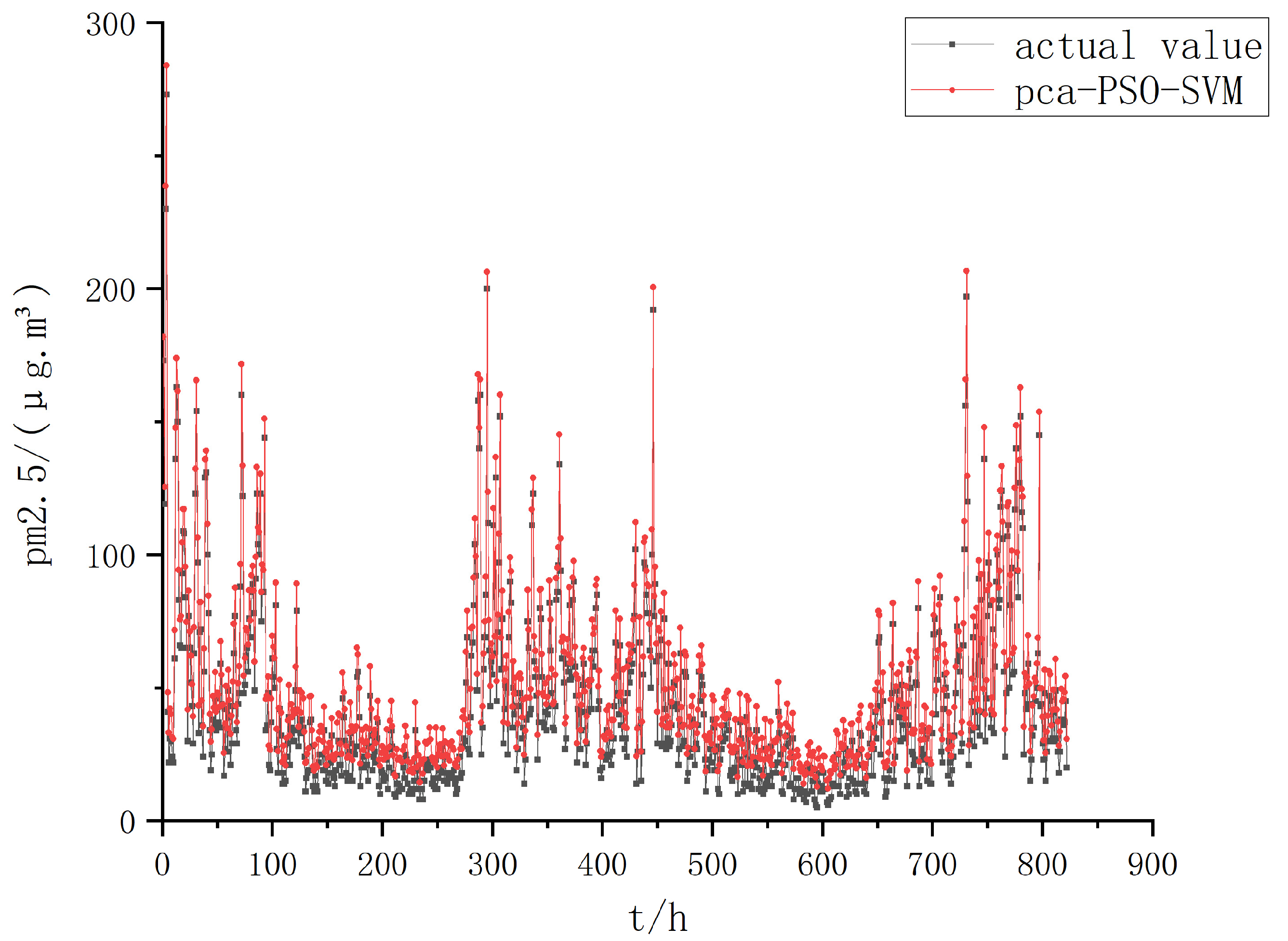
4.2. Comparison of Prediction Results

Figure 4 shows that the PM2.5 concentration changes significantly at different time points. Other different pollutants may affect its changes. Therefore, it is crucial to analyse and predict the PM2.5 concentration. To better understand the prediction accuracy of different methods in predicting the PM2.5 concentration, different methods were used to compare the same batch of sampling samples and calculate the prediction errors. Figure 4 depicts the results of the PCA–GA–SVM method’s prediction of the PM2.5 concentration. Figure 5 depicts the PCA–PSO–SVM network method’s PM2.5 prediction results. Figure 6 depicts the PCA–SSA–SVM network method’s PM2.5 prediction results.

Figure 4 demonstrates that the PCA–GA–SVM method predicts a deviation in the PM2.5 concentration at a certain point in time. For example, the deviation is prominent in the time point of 700 ~ 800, but the prediction process is consistent with the actual value. Compared with the PCA–PSO–SVM method in Figure 6, the prediction accuracy of PM2.5 concentration is higher, and the PCA–PSO–SVM method is biased in regard to predicting the PM2.5 concentration at a certain point. Figure 5 exhibits a specific deviation between the predicted PM2.5 concentration at time points between 300 and 400 and the actual value, which also occurs at time points between 700 and 800. Therefore, the prediction accuracy of the PCA–PSO–SVM method still needs to be improved. The simulation experiments also prove that the PCA–SSA–SVM method has a faster learning speed and higher prediction accuracy. It fully uses the sparrow position to represent parameters c and g of SVM to optimise the SVM network.

Figure 5 shows that the PM2.5 concentration predicted by PCA–SSA–SVM is basically consistent with the actual value, and there will be a slight prediction deviation at a single point. The prediction trend shows that the PM2.5 concentration is well predicted. Therefore, it demonstrates that the proposed method has a good effect in the prediction of PM2.5 concentration. Figure 7 reveals that the overall effect of this method in predicting PM2.5 concentration is better than that of other methods.

4.3. Optimised SSA–SVM Compared with Other Models

The SVM relies on two crucial parameters: the penalty parameter, c; and the kernel function, g. These parameters significantly impact the prediction model’s accuracy. Consequently, selecting optimal values for c and g is pivotal in SVM optimisation. This work proposes utilising the SSA algorithm to optimise the SVM, aligning with the original objective. Following multiple iterations of debugging, the parameters of the sparrow algorithm were established as the subsequent values: the quantity of sparrows, denoted as N, is equal to 20.

The maximum number of iterations (Max-iteration) is 200; the penalty parameter (c) and kernel function (g) of SVM are in the range of [2–5, 25]. The best parameters finally obtained are c = 3.4825 and g = 0.0312. In other words, with these optimal c and g values, the SSA–SVM model has the highest accuracy.

To examine the prediction performance of the SSA–SVM model, partial least squares (PLS) was selected to compare with the SVM model optimised by the GA and particle swarm algorithm (PSO). Random time series were selected as input variables of several models; the best parameters of the GA–SVM were c = 7.2218 and g = 0.0435, and the best parameters of the PSO–SVM were c = 17.1872 and g = 0.0512. The best parameters were substituted into the model to predict the PM2.5 concentration. The optimal PM2.5 prediction model is selected by comparing the accuracy and time consumption of each model.

While comparing the time series data PM2.5 prediction accuracy as input variables, we observed that the SSA–SVM algorithm has an accuracy improvement of 5.83% compared to the PLS algorithm; a 6.03% improvement compared with the SVM algorithm; and a higher accuracy of 2.68% and 5.2% from the GA–SVM algorithm and PSO–SVM algorithm, respectively. Hence, SSA–SVM is the best prediction model for PM2.5. Figure 8 demonstrates that the fitness value of the SSA–SVM algorithm gradually approaches the optimal value as the number of fitness iterations increases and remains stable after reaching the lowest point.

Table 3. Factor matrix of each component.

Modelling Methods	MAE	RMSE	R²	Time/s
Full-PLS	6.25	8.14	0.9306	6.1321
PCA–PLS	1.86	3.76	0.9598	5.7554
Full-SVM	0.843	1.054	0.9286	4.2311
PCA–SVM	0.339	0.401	0.9571	3.9871
Full–GA–SVM	2.65	2.97	0.9621	16.3269
PCA–GA–SVM	2.028	1.53	0.9798	13.1432
Full–PSO–SVM	7.48	8.84	0.9369	13.2411
PCA–PSO–SVM	2.221	3.16	0.9649	10.2311
Full–SSA–SVM	0.59	0.92	0.9889	6.0569
PCA–SSA–SVM	0.084	0.11	0.9996	4.1121

demonstrates the accuracy comparison of PM2.5 prediction by using five different prediction models, while using time series as input variables. When all the time series are used as input, the SSA–SVM model’s prediction of PM2.5 can fulfil the prediction requirements: R² = 0.9889, and RMSE = 0.0092. It takes 6.0569 s to complete the task. Although the two classic regression models, SVM and PLS, have shorter computation times, their accuracy is low.

The accuracy of GA–SVM and PSO–SVM is improved compared with traditional SVM; however, it is still lower than the SSA–SVM model proposed in this paper and takes too long. Table 2 intuitively shows the prediction effects of different models on PM2.5 data. The prediction effect is ranked as follows: SSA–SVM > GA–SVM > PSO–SVM > PLS > SVM. Furthermore, PCA played a prominent role in reducing the dimensionality of data.

The findings show that the SSA algorithm has more advantages than the GA and PSO algorithms in optimising SVM. It is not easy to fall into local optimality, but it effectively improves the accuracy of PM2.5 prediction, and the iteration time is significantly shortened. Although the PLS and SVM algorithms are short in time, their prediction accuracy is low, and they have no advantage in the prediction of PM2.5.

Figure 9 depicts the trend effects of the three methods in predicting the PM2.5 concentration. The prediction results of PCA–SSA–SVM are closer to the actual PM2.5 concentration value. Therefore, applying the proposed PCA–SSA–SVM method in predicting atmospheric PM2.5 concentration is proved to be effective. Table 2 presents the calculation times of different prediction algorithms. The table shows that the calculation time of the proposed algorithm is 4.1121, and its calculation time is the fastest among the four algorithms. Therefore, the proposed algorithm takes the shortest time and has the slightest error.

5. Conclusions

This paper predicts the atmospheric PM2.5 concentration by using the improved SSA–SVM method. The primary factors affecting atmospheric change were extracted from the monitored data of PM2.5, PM10, SO₂, NO₂, CO, O₃, temperature and humidity, using the PCA method, and the variables PM10, NO₂, SO₂ and PM2.5 4 were determined as the research variables to be established by the cumulative contribution rate. The correlation between the PM2.5 concentration and other variables was studied, and the SSA–SVM method was used to predict the PM2.5 concentration. The simulation results reveal that the SSA–SVM method solves the problem of high-dimensional data redundancy in atmospheric data and completes the more accurate prediction of PM2.5 concentration in a short time. Compared with PCA–SSA–SVM, PCA–GA–SVM, PCA–PSO–SVM and PCA–PLS–SVM prediction methods, PCA–SSA–SVM can update the network model parameters through the training data of different batch sizes on the premise of ensuring the prediction accuracy of the PM2.5 concentration. Furthermore, it can realise more rapid, stable and accurate predictions; make up for the shortcomings of other proposed prediction methods; and verify the effectiveness and practicability of the proposed method.

In general, the model proposed in this paper is suitable for processing the data of multiple monitoring points in the target region as the input of time series and is favourable for dealing with high-dimensional atmospheric data. It can incorporate the interactions of air pollutants from multiple monitoring points into the prediction system. The proposed work has some limitations:

(1) The training data of this model came from multiple monitoring sites; (2) the work is based on only one province (Jilin), and the authors hope to collect more monitoring data from other regions to verify the generality of this work; and (3) more factors, such as geomorphology and spatial conditions, must be considered in future works. Therefore, the regularity of air pollutant data can be better determined, and more accurate prediction results can be obtained. Despite its limitations, the PCA–SSA–SVM method presented here can help predict pollution, such as air pollutant concentrations over complex air pollution data and larger areas containing monitoring stations.

References

1. Stern, A.C. Air Pollution: The Effects of Air Pollution; Elsevier: Amsterdam, The Netherlands, 1977. [Google Scholar]
2. Brunekreef, B.; Holgate, S.T. Air pollution and health. Lancet 2002, 360, 1233–1242. [Google Scholar] [PubMed]
3. Chow, J.C. Health effects of fine particulate air pollution: Lines that connect. J. Air Waste Manag. Assoc. 2006, 56, 707–708. [Google Scholar]
4. Dominici, F.; Peng, R.D.; Bell, M.L.; Pham, L.; McDermott, A.; Zeger, S.L.; Samet, J.M. Fine particulate air pollution and hospital admission for cardiovascular and respiratory diseases. JAMA 2006, 295, 1127–1134. [Google Scholar] [PubMed]
5. Xing, Y.F.; Xu, Y.H.; Shi, M.H.; Lian, Y.X. The impact of PM2.5 on the human respiratory system. J. Thoracic. Dis. 2016, 8, 69. [Google Scholar]
6. Brook, R.D.; Rajagopalan, S.; Pope, C.A.; Brook, J.R.; Bhatnagar, A.; Diez-Roux, A.V.; Holguin, F.; Hong, Y.; Luepker, R.V.; Mittleman, M.A.; et al. Particulate matter air pollution and cardiovascular disease: An update to the scientific statement from the american heart association. Circulation 2010, 121, 2331–2378. [Google Scholar] [CrossRef] [PubMed]
7. Pope, C.A.; Burnett, R.T.; Thun, M.J.; Calle, E.E.; Krewski, D.; Ito, K.; Thurston, G.D. Lung cancer, cardiopulmonary mortality, and long-term exposure to fine particulate air pollution. JAMA 2002, 287, 1132–1141. [Google Scholar] [CrossRef]
8. Li, T.; Shen, H.; Zeng, C.; Yuan, Q.; Zhang, L. Point-surface fusion of station measurements and satellite observations for mapping PM2.5 distribution in China: Methods and assessment. Atmos. Environ. 2017, 152, 477–489. [Google Scholar]
9. James, D.E.; Chambers, J.A.; Kalma, J.D.; Bridgman, H.A. Air quality prediction in urban and semi-urban regions with generalised input-output analysis: The hunter region, australia. Urban Ecol. 1985, 9, 25–44. [Google Scholar]
10. Bruckman, L. Overview of the enhanced geocoded emissions modeling and projection (enhanced gemap) system. In Proceeding of the Air & Waste Management Association’s Regional Photochemical Measurements and Modeling Studies Conference, San Diego, CA, USA, 8–12 November 1993. [Google Scholar]
11. Wang, W.; Zhao, S.; Jiao, L.; Taylor, M.; Zhang, B.; Xu, G.; Hou, H. Estimation of PM2.5 concentrations in China using a spatial back propagation neural network. Sci. Rep. 2019, 9, 13788. [Google Scholar] [CrossRef]
12. Wen, C.; Liu, S.; Yao, X.; Peng, L.; Li, X.; Hu, Y.; Chi, T. A novel spatiotemporal convolutional long short-term neural network for air pollution prediction. Sci. Total Environ. 2019, 654, 1091–1099. [Google Scholar] [CrossRef]
13. Mao, W.; Wang, W.; Jiao, L.; Zhao, S.; Liu, A. Modeling air quality prediction using a deep learning approach: Method optimisation and evaluation. Sustain. Cities Soc. 2020, 65, 102567. [Google Scholar] [CrossRef]
14. Geng, G.; Zhang, Q.; Martin, R.V.; van Donkelaar, A.; Huo, H.; Che, H.; Lin, J.; He, K. Estimating long-term PM2.5 concentrations in China using satellite-based aerosol optical depth and a chemical transport model. Remote Sens. Environ. 2015, 166, 262–270. [Google Scholar] [CrossRef]
15. Stern, R.; Builtjes, P.; Schaap, M.; Timmermans, R.; Vautard, R.; Hodzic, A.; Memmesheimer, M.; Feldmann, H.; Renner, E.; Wolke, R. A model inter-comparison study focussing on episodes with elevated PM10 concentrations. Atmos. Environ. 2008, 42, 4567–4588. [Google Scholar] [CrossRef]
16. Wang, J.; Bai, L.; Wang, S.; Wang, C. Research and application of the hybrid forecasting model based on secondary denoising and multi-objective optimisation for air pollution early warning system. J. Clean. Prod. 2019, 234, 54–70. [Google Scholar] [CrossRef]
17. Pan, L.; Sun, B.; Wang, W. City air quality forecasting and impact factors analysis based on grey model. Procedia Eng. 2011, 12, 74–79. [Google Scholar] [CrossRef]
18. Li, T.; Shen, H.; Yuan, Q.; Zhang, L. Geographically and temporally weighted neural networks for satellite-based mapping of ground-level PM2.5. ISPRS J. Photogramm. Remote Sens. 2020, 167, 178–188. [Google Scholar]
19. Yuan, Q.; Shen, H.; Li, T.; Li, Z.; Li, S.; Jiang, Y.; Xu, H.; Tan, W.; Yang, Q.; Wang, J.; et al. Deep learning in environmental remote sensing: Achievements and challenges. Remote Sens. Environ. 2020, 241, 111716. [Google Scholar] [CrossRef]
20. Lv, B.; Cai, J.; Xu, B.; Bai, Y. Understanding the rising phase of the PM2.5 concentration evolution in large China cities. Sci. Rep. 2017, 7, 46456. [Google Scholar] [CrossRef]
21. Gupta, P.; Christopher, S.A. Particulate matter air quality assessment using integrated surface, satellite, and meteorological products: 2. A neural network approach. J. Geophys. Res. Atmos. 2009, 114, 1–14. [Google Scholar]
22. Zhang, G.; Lu, H.; Dong, J.; Poslad, S.; Li, R.; Zhang, X.; Rui, X. A framework to predict high-resolution spatiotemporal PM2.5 distributions using a deep-learning model: A case study of Shijiazhuang, China. Remote Sens. 2020, 12, 2825. [Google Scholar]
23. Fan, Z.; Zhan, Q.; Yang, C.; Liu, H.; Bilal, M. Estimating PM2.5 concentrations using spatially local Xgboost based on full-covered SARA AOD at the urban scale. Remote Sens. 2020, 12, 3368. [Google Scholar] [CrossRef]
24. Shen, H.; Jiang, Y.; Li, T.; Cheng, Q.; Zeng, C.; Zhang, L. Deep learning-based air temperature mapping by fusing remote sensing, station, simulation and socioeconomic data. Remote Sens. Environ. 2020, 240, 111692. [Google Scholar] [CrossRef]
25. Wan, R.; Mei, S.; Wang, J.; Liu, M.; Yang, F. Multivariate temporal convolutional network: A deep neural networks approach for multivariate time series forecasting. Electronics 2019, 8, 876. [Google Scholar] [CrossRef]
26. Qi, Y.; Li, Q.; Karimian, H.; Liu, D. A hybrid model for spatiotemporal forecasting of PM2.5 based on graph convolutional neural network and long short-term memory. Sci. Total Environ. 2019, 664, 1–10. [Google Scholar] [PubMed]
27. Han, L.; Zhao, J.; Gao, Y.; Gu, Z.; Xin, K.; Zhang, J. Spatial distribution characteristics of PM2.5 and PM10 in Xi’an city predicted by land use regression models. Sustain. Cities Soc. 2020, 61, 102329. [Google Scholar]
28. Stadlober, E.; Hörmann, S.; Pfeiler, B. Quality and performance of a PM10 daily forecasting model. Atmos. Environ. 2008, 42, 1098–1109. [Google Scholar] [CrossRef]
29. Perez, P.; Reyes, J. An integrated neural network model for PM10 forecasting. Atmos. Environ. 2006, 40, 2845–2851. [Google Scholar] [CrossRef]
30. Suárez Sánchez, A.; García Nieto, P.J.; Riesgo Fernández, P.; Del Coz Díaz, J.J.; Iglesias-Rodríguez, F.J. Application of an SVM-based regression model to the air quality study at local scale in the Avilés urban area (Spain). Math. Comput. Model. 2011, 54, 1453–1466. [Google Scholar]
31. Gariazzo, C.; Carlino, G.; Silibello, C.; Renzi, M.; Finardi, S.; Pepe, N.; Radice, P.; Forastiere, F.; Michelozzi, P.; Viegi, G.; et al. A multi-city air pollution population exposure study: Combined use of chemical-transport and random-forest models with dynamic population data. Sci. Total Environ. 2020, 724, 138102. [Google Scholar]
32. Danesh Yazdi, M.; Kuang, Z.; Dimakopoulou, K.; Barratt, B.; Suel, E.; Amini, H.; Lyapustin, A.; Katsouyanni, K.; Schwartz, J. Predicting fine particulate matter (PM2.5) in the greater London area: An ensemble approach using machine learning methods. Remote Sens. 2020, 12, 914. [Google Scholar] [CrossRef]
33. Schneider, R.; Vicedo-Cabrera, A.M.; Sera, F.; Masselot, P.; Stafoggia, M.; de Hoogh, K.; Kloog, I.; Reis, S.; Vieno, M.; Gasparrini, A. A satellite-based spatio-temporal machine learning model to reconstruct daily PM2.5 concentrations across Great Britain. Remote Sens. 2020, 12, 3803. [Google Scholar]
34. Zhou, Q.; Jiang, H.; Wang, J.; Zhou, J. A hybrid model for PM2.5 forecasting based on ensemble empirical mode decomposition and a general regression neural network. Sci. Total Environ. 2014, 496, 264–274. [Google Scholar] [CrossRef] [PubMed]
35. Chang-Hoi, H.; Park, I.; Oh, H.; Gim, H.; Hur, S.; Kim, J.; Choi, D. Development of a PM2.5 prediction model using a recurrent neural network algorithm for the Seoul metropolitan area, Republic of Korea. Atmos. Environ. 2021, 245, 118021. [Google Scholar]
36. Wu, S.; Feng, Q.; Du, Y.; Li, X.D. Artificial neural network models for daily PM10 air pollution index prediction in the urban area of Wuhan, China. Environ. Eng. Sci. 2011, 28, 357–363. [Google Scholar] [CrossRef]
37. Wei, G.; Zhao, J.; Yu, Z.; Feng, Y.; Li, G.; Sun, X. An effective gas sensor array optimisation method based on random forest. In Proceedings of the 2018 IEEE Sensors, New Delhi, India, 28–31 October 2018; pp. 1–4. [Google Scholar]
38. Xu, Y.; Zhao, X.; Chen, Y.; Zhao, W. Research on a mixed gas recognition and concentration detection algorithm based on a metal oxide semiconductor olfactory system sensor array. Sensors 2018, 18, 3264. [Google Scholar] [PubMed]
39. Boateng, E.Y.; Otoo, J.; Abaye, D.A. Basic tenets of classification algorithms K-nearest-neighbor, support vector machine, random forest and neural network: A review. J. Data Anal. Inf. Process. 2020, 8, 341–357. [Google Scholar]
40. Sánchez, V.D.A. Advanced support vector machines and kernel methods. Neurocomputing 2003, 55, 5–20. [Google Scholar] [CrossRef]
41. Zhao, X.; Li, P.; Xiao, K.; Meng, X.; Han, L.; Yu, C. Sensor Drift Compensation Based on the Improved LSTM and SVM Multi-Class Ensemble Learning Models. Sensors 2019, 19, 3844. [Google Scholar]
42. Tao, Z.; Huiling, L.; Wenwen, W.; Xia, Y. GA–SVM-based feature selection and parameter optimisation in hospitalisation expense modeling. Appl. Soft Comput. 2019, 75, 323–332. [Google Scholar] [CrossRef]
43. Huang, S.; Zheng, X.; Ma, L.; Wang, H.; Huang, Q.; Leng, G.; Meng, E.; Guo, Y. Quantitative contribution of climate change and human activities to vegetation cover variations based on GA–SVM model. J. Hydrol. 2020, 584, 124687. [Google Scholar] [CrossRef]
44. Cuong-Le, T.; Nghia-Nguyen, T.; Khatir, S.; Trong-Nguyen, P.; Mirjalili, S.; Nguyen, K.D. An efficient approach for damage identification based on improved machine learning using PSO–SVM. Eng. Comput. 2022, 38, 3069–3084. [Google Scholar]
45. Zhang, L.; Shi, B.; Zhu, H.; Yu, X.B.; Han, H.; Fan, X. PSO–SVM-based deep displacement prediction of Majiagou landslide considering the deformation hysteresis effect. Landslides 2021, 18, 179–193. [Google Scholar] [CrossRef]
46. Pan, M.; Li, C.; Gao, R.; Huang, Y.; You, H.; Gu, T.; Qin, F. Photovoltaic power forecasting based on a support vector machine with improved ant colony optimisation. J. Clean. Prod. 2020, 277, 123948. [Google Scholar] [CrossRef]
47. Lewis, M. A The whale optimisation algorithm. Adv. Eng. Softw. 2016, 95, 51–67. [Google Scholar]
48. Xue, J.K.; Shen, B. A novel swarm intelligence optimisation approach: Sparrow search algorithm. Syst. Sci. Control. Eng. 2020, 8, 22–34. [Google Scholar]
49. Ye, Y.B.; Li, R.C.; Xie, M.; Wang, Z.; Ba, Q. A state evaluation method for a relay protection device based on SSA–SVM. Power Syst. Prot. Control. 2022, 50, 171–178. (In Chinese) [Google Scholar]
50. Yu, S.; Hu, D.; Tang, C.; Zhang, C.; Tang, W. MSSA-SVM Transformer Fault Diagnosis Method Based on TLR-ADASYN Balanced Data Set. High Volt. Eng. 2021, 47, 3845–3853. (In Chinese) [Google Scholar]
51. Song, J.; Cong, Q.M.; Yang, S.S.; Yang, J. Improved sparrow search algorithm for water quality prediction in RBF neural networks. Comput. Syst. 2023, 4, 255–261. [Google Scholar]
52. Li, N.; Xue, J.K.; Shu, H.S. UA V trajectory planning based on adaptive t-distribution variational sparrow search algorithm. J. Donghua Univ. (Nat. Sci. Ed.) 2022, 48, 69–74. [Google Scholar]
Figure 1. Jilin’s 30 air-monitoring stations’ variables.
Sustainability 16 00832 g001
Figure 2. Component characteristic contribution value.
Sustainability 16 00832 g002
Figure 3. Flowchart of the initialisation.
Sustainability 16 00832 g003
Figure 4. PM2.5’s actual value.
Sustainability 16 00832 g004
Figure 5. Prediction of PM2.5 concentration based on the PCA–GA–SVM method.
Sustainability 16 00832 g005
Figure 6. Prediction of PM2.5 concentration based on the PCA–PSO–SVM method.
Sustainability 16 00832 g006
Figure 7. Prediction of PM2.5 concentration based on the PCA–SSA–SVM method.
Sustainability 16 00832 g007
Figure 8. SSA–SVM convergence curve.
Sustainability 16 00832 g008
Figure 9. Prediction results of PM2.5 concentration using three methods.
Sustainability 16 00832 g009