Review of Bridge Structure Damping Model and Identification Method

Abstract

Damping is a fundamental characteristic of bridge structures, reflecting their ability to dissipate energy during vibration. In the design and maintenance of bridges, the damping ratio has a direct impact on the safety and service life of the structure, thus affecting its sustainability. Currently, there is no suitable theoretical method for estimating structural damping at the design stage. Therefore, the modal damping ratio of a completed or under-construction bridge can only be obtained through field dynamic tests to ensure compliance with design specifications. To summarize the latest research findings on bridge structure damping models and identification methods, and to advance the development of damping identification techniques, this paper provides an in-depth review from several perspectives: Firstly, it offers a comprehensive analysis of the theoretical framework for structural damping. Secondly, it summarizes the damping models proposed by researchers from various countries. Thirdly, it reviews the research progress on identifying the modal damping ratio of bridge structures using time domain, frequency domain, and time-frequency domain methods based on environmental excitation. It also summarizes the methods and current status of identifying the modal damping ratio using artificial excitation. Finally, the future prospects and conclusions are discussed from three aspects: damping theory, test and identification method and data processing. This research and summary provide a solid theoretical foundation for advancing bridge structural damping theory and identification methods and offer valuable references for bridge operation and maintenance, as well as damage identification. From the perspective of modal parameter identification, it provides a theoretical basis for the sustainable development of bridges.

1. Introduction

Since the reform and opening-up, China’s economic development has accelerated rapidly, leading to the flourishing of large-scale civil infrastructure projects [1,2,3,4]. Bridges, as an essential component of transportation infrastructure, play a crucial role in enhancing urban efficiency and supporting stable national economic development. The construction of bridges not only reduces travel time but also facilitates trade and commercial activities between regions, injecting new vitality into economic growth. According to the Statistical Communiqué on the Development of the Transportation Industry in 2023 issued by the Ministry of Transport of China, by the end of 2023, China had 1.0793 million highway bridges with a total length of 95.2882 million continuous meters. This represents an increase of 46,100 bridges and 95.233 million continuous meters compared to the end of the previous year. This total includes 10,239 super-large bridges of 18.7301 million continuous meters and 177.77 million bridges of 49.9437 million continuous meters.

As the boom in traditional infrastructure construction in China gradually subsides, the degradation of bridge materials and the accumulation of structural damage have become increasingly prominent issues. Coupled with the rapid advancement of new infrastructure and the increase in industrial heavy equipment, the number of overweight vehicles has grown, making bridge operating conditions more challenging. The combined effects of environmental changes and adverse events have further exacerbated issues such as the decline in bridge durability [5,6], the weakening of load-bearing capacity [7], and the reduction in resistance [8]. If these problems are not promptly detected through effective structural health monitoring and addressed with appropriate bridge maintenance measures, they may lead to a shortened service life of bridges in mild cases, and in severe cases, cause structural damage or even collapse, resulting in catastrophic accidents. Such incidents would not only have a serious impact on the social economy and people’s lives but also directly contradict the basic principles of sustainable development. In this context, damping is one of the key parameters of bridge dynamic behavior, and its impact on bridge health and sustainability cannot be ignored. Damping not only affects the response of the bridge to dynamic loads but also determines the energy dissipation capacity of the bridge when subjected to external shocks. In the long run, the change in damping characteristics reflects the aging degree of bridge materials and the accumulation of structural damage. For example, material aging will lead to a decrease in the damping coefficient, thereby reducing the bridge’s ability to absorb external shocks and increasing the risk of structural fatigue damage. On the other hand, when the bridge structure is damaged, the local damping characteristics will change, which can be used as an important indicator of early damage detection. By continuously monitoring the change in damping characteristics, potential structural problems can be found in time, which provides a scientific basis for preventive maintenance.

For bridge structures, changes in dynamic characteristics are often reflected in variations in the modal parameters of the structure. The modal parameters of the structure [9] include vibration modes, natural frequencies, and modal damping ratios. Additionally, modal parameters characterize the regular characteristics of bridge structures under load and environmental conditions, providing essential data for finite element model updating, damage identification, and structural state assessment. Therefore, to accurately understand the service performance and operational status of a bridge, precise identification of the modal parameters is essential.

Damping is a key parameter for the dynamic analysis and damage identification of structures, including wind and seismic resistance. Accurately determining the structural damping is crucial. Damping refers to the physical phenomenon where a structure experiences resistance during vibration, causing the amplitude to gradually decrease and eventually stabilize. It represents the objective description of energy dissipation during structural vibration. Based on energy dissipation mechanisms, damping is generally classified into system damping, internal damping, and external damping. System damping pertains to the energy dissipation components installed within the structure [10], such as dampers and rubber bearings. These devices absorb and disperse vibration energy to reduce structural amplitude and shorten the duration of vibrations. Internal damping reflects the structure’s inherent ability to dissipate vibration energy and is further divided into material damping and structural damping. Material damping arises from the friction between micro-particles within the material and between macro-phase interfaces and micro-cracks during vibration. Structural damping is influenced by the structural form, the configuration of the structure, the connection states between components, and other factors. During vibration, relative slip between components generates friction, which leads to energy dissipation and reduction in vibration amplitude—this constitutes structural damping. External damping describes energy dissipation to the surrounding medium and can be categorized into medium damping and radiation damping. Medium damping refers to energy dissipation effects due to interactions between structural vibrations and external media, such as aerodynamic and hydrodynamic damping, depending on the medium involved. Radiation damping primarily involves energy dissipation through the foundation during vibrations, including energy loss in waveform and friction between the foundation and the surrounding soil. This paper focuses on internal and external damping, excluding the damping from additional damping devices.

The damping of bridge structures primarily arises from internal and external sources. Its mechanism is highly complex, and no mathematical model currently exists that can fully and accurately describe this mechanism. Due to the inherent characteristics of bridge structures, they are often modeled as linear vibration systems, with their vibration responses represented by the linear superposition of multiple modes. Consequently, the modal damping ratio is commonly used to represent the overall effect of various damping mechanisms on a bridge structure. The modal damping ratio [11] reflects the modal damping ratio of the structure during its vibration in the first-order mode, indicating the extent of vibration energy dissipation in this mode. A higher modal damping ratio corresponds to greater energy dissipation per cycle and more rapid attenuation of the structural amplitude.

Physical parameters such as the mass and stiffness of a bridge structure can be calculated to obtain more accurate results, but accurately calculating damping remains challenging. Modal analysis [12] is considered the most reliable method for determining damping. Modal analysis methods can be divided into experimental modal analysis [13] and operational modal analysis [14] based on different excitation techniques. Currently, operational modal analysis is widely used. This method’s main advantage is that it does not require artificial excitation; instead, it uses the bridge structure’s response to environmental excitation to identify damping, making it an output-only identification method. Because the operational modal analysis needs long-term monitoring, it may contain abnormal data. It is very important to eliminate these abnormal data [15]. It generally assumes that the input is Gaussian white noise and the system is time-invariant. However, environmental excitation for a designed bridge is highly complex, including factors such as vehicle loads and wind loads, which are typically non-stationary colored noise rather than Gaussian white noise. Additionally, vehicle loads alter the bridge’s characteristics, and vehicle-bridge coupling vibrations mix the bridge’s vibration signals with those of the vehicle, increasing the complexity of signal analysis. The amplitude of the bridge structure under environmental excitation is small, resulting in a low signal-to-noise ratio for the collected response signals. These factors cause significant fluctuations in the identified modal damping ratio, making it challenging to provide reliable references for engineering construction. In order to monitor the dynamic data of the bridge structure in real time, the three-dimensional coordinates of the actual bridge are usually collected to construct the point cloud model, and the dynamic displacement of the bridge structure is displayed on the point cloud model [16]. In contrast, experimental modal analysis, which uses artificial excitation methods such as hammering, exciters, jumping excitation, or rocket launching, can produce greater amplitude in the bridge structure and obtain higher signal-to-noise ratio response signals. This allows for more reliable identification of modal parameters, particularly the modal damping ratio. For many medium and small-span bridges, rapid structural detection technology has become the primary means of evaluating service safety. By collecting vibration responses from key positions on the bridge using methods like hammering and exciters, and analyzing input and output data in real time, this technology provides fast, accurate, and comprehensive assessments. However, for large bridge tests, substantial excitation equipment is required, and traffic closure may be necessary, making it difficult and costly to accurately identify the modal damping ratio.

The bridge has a prominent wind-induced vibration problem, so the value of the modal damping ratio of the bridge is particularly important in the design stage. Accurate determination of the damping of the bridge is the theoretical basis for quantitative analysis of structural dynamic response and evaluation of structural wind and seismic resistance. It is the main means to test the effectiveness of structural vibration isolation measures. It is an important basis for revising the structural design code. At present, the design values of damping ratios of different bridge structures given by China’s specifications ‘Code for Wind Resistance Design of Highway Bridges’ [17] and ‘Code for Seismic Design of Highway Bridges’ [18] are not the same, and their design values are determined according to experience. It is necessary to revise the design value of the specification based on the measured value of the damping ratio of the existing bridge. In short, how to accurately identify the damping of the bridge structure has important engineering significance for evaluating the dynamic characteristics of the structure, and is an important research direction in the field of civil engineering.

This paper systematically reviews the damping models proposed by scholars from various countries, analyzes the research progress and application status of bridge structure modal damping ratio identification methods based on environmental and artificial excitation, and finally, outlines future research directions in terms of damping theory, identification methods, and data processing techniques. This not only lays a solid foundation for theoretical development in this field but also provides a new idea for the development of damping ratio identification of bridge structures. By comprehensively analyzing the advantages and disadvantages of various identification methods, this paper aims to promote the further improvement of bridge structure damping theory and provides important technical support and valuable reference materials for key areas such as bridge operation and maintenance, damage identification and safety assessment.

2. Damping Model and Damping Characteristics of Bridge Structure

Damping is a parameter that reflects the characteristics of energy dissipation during the vibration of structural systems. The energy consumption during actual structural vibration is multifaceted, with varying degrees of influence. To accurately characterize damping, a reasonable expression method must be identified. After nearly a century of research, scholars from various countries have proposed several methods for expressing damping. In practical engineering applications, to reflect the damping mechanism in structures and facilitate dynamic analysis, damping is typically simplified into a corresponding theoretical model with mathematical expressions to describe the damping force. The damping models proposed in existing research include the viscous damping model, hysteresis damping model, complex damping model, Coulomb damping model, convolution damping model, and aerodynamic damping model.

2.1. Viscous Damping Model

The basic assumption of the viscous damping model [19] is that the magnitude of the damping force is proportional to the velocity, and its expression in the single-degree-of-freedom system is shown in Equation (1). In structural dynamics, the viscous damping model simplifies the analysis of the vibration system. Due to the convenience of mathematical calculation, the model has become the most widely used damping model in theoretical research and practical application. For the multi-degree-of-freedom vibration system, a viscous proportional damping model can be established. The original simultaneous vibration equations are decoupled into independent single-degree-of-freedom structural vibration equations by using the principle of mode superposition, and then the modal parameters such as frequency, modal damping ratio and vibration mode of the structure are calculated. Although the viscous damping model is idealized, it can still approximately describe the damping behavior in the actual bridge structure. In bridge structures, the damping effect is often mainly caused by friction or air resistance inside the material, and these resistances are usually proportional to the speed.

$$f_d^{vi}=-c\dot{x}$$

(1)

where $f_d^{vi}$ is the damping force; $c$ is the damping coefficient; $\dot{x}$ is the vibration velocity of the structure.

When the viscous damping model is used, the motion equation of the multi-degree-of-freedom structure is:

$$M\ddot{x}\left(t\right)+C\dot{x}\left(t\right)+Kx\left(t\right)=f\left(t\right)$$

(2)

where $x\left(t\right)={\left[\begin{array}{cccc}{x}_1\left(t\right)& x_2\left(t\right)& \cdots & x_N\left(t\right)\end{array}\right]}^{\mathrm{T}}\in {\mathrm{R}}^{N\times 1}$ is the structural displacement vector, $\dot{x}\left(t\right)\in {\mathrm{R}}^{N\times 1}$ and $\ddot{x}\left(t\right)\in {\mathrm{R}}^{N\times 1}$ are the structural velocity and acceleration vectors, respectively; $M\in {\mathrm{R}}^{N\times N}$, $C\in {\mathrm{R}}^{N\times N}$ and $K\in {\mathrm{R}}^{N\times N}$ are the mass, damping and stiffness matrices of the structure, respectively. $f\left(t\right)=\left[\begin{array}{cccc}{f}_1\left(t\right)& f_2\left(t\right)& \cdots & f_N\left(t\right)\end{array}\right]\in {\mathrm{R}}^{N\times 1}$ is the excitation force vector; $N$ is the number of degrees of freedom of the structure; the superscript $\mathrm{T}$ denotes the transpose operation.

The advantage of the viscous damping model is the convenience of theoretical analysis. Because the damping force is proportional to the relative velocity, the motion equation is a linear equation. In harmonic or non-harmonic vibration, the response of the structure can be written directly, which is easy to calculate, so it becomes the most widely used damping model. The current damping identification theory is also based on the damping model.

When the damping matrix $C$ adopts different expressions, there are different viscous damping models. In order to facilitate the modal analysis method, the damping matrix generally adopts the proportional damping model [20], that is, the damping matrix can be orthogonalized into a diagonal matrix by modal vector. Scholars from various countries have proposed some proportional damping models, among which the most representative ones are the Rayleigh damping model, the Caughey damping model, the Wilson–Penzien damping and the Clough damping model.

2.1.1. Rayleigh Damping Model

The Rayleigh damping model is one of the most commonly used damping models for the vibration response analysis of multi-degree-of-freedom systems. This model is widely adopted due to the convenience it offers in calculating multi-degree-of-freedom systems. The expression for Rayleigh damping is given in Equation (3). The model assumes that damping is a linear combination of mass and stiffness, allowing the damping matrix to be diagonalized similarly to the mass and stiffness matrices. Consequently, the motion equation of the multi-degree-of-freedom system can be decoupled into the equations of motion for independent single-degree-of-freedom systems. The solutions for the single-degree-of-freedom systems are then combined to obtain the solution for the multi-degree-of-freedom system using the mode superposition method.

$$C_{ra}=\alpha M+\beta K$$

(3)

where $\alpha$ and $\beta$ are coefficients, which can be determined according to the actual measured modal damping ratio.

The viscous modal damping ratio is defined as:

$$\xi ={\displaystyle \frac{c}{c_c}}={\displaystyle \frac{c}{2m\omega }}$$

(4)

where $c$ is damping; $c_c$ is the critical damping; $m$ is mass; $\omega$ is the undamped natural frequency.

According to the definition of viscous modal damping ratio, the relationship between modal damping ratio and frequency can be obtained from Rayleigh damping:

$${\xi }_n={\displaystyle \frac{\alpha }{2{\omega }_n}}+{\displaystyle \frac{\beta {\omega }_n}{2}}$$

(5)

where ${\xi }_n$ is the nth-order modal damping ratio; ${\omega }_n$ is the natural frequency of the nth mode.

If the natural frequencies ${\omega }_i$ and ${\omega }_j$ of any two modes and the corresponding damping ratios ${\xi }_i$ and ${\xi }_j$ are known, the coefficients $\alpha$ and $\beta$ of two Rayleigh dampings can be obtained by a pair of simultaneous equations.

$$\left(\begin{array}{c}\alpha \\ \beta \end{array}\right)=2{\displaystyle \frac{{\omega }_i{\omega }_j}{{\omega }_i^2-{\omega }_j^2}}\left(\begin{array}{cc}{\omega }_i& -{\omega }_j\\ -{\displaystyle \raisebox{1ex}{$1$}\!\left/ \!\raisebox{-1ex}{${\omega }_i$}\right.}& {\displaystyle \raisebox{1ex}{$1$}\!\left/ \!\raisebox{-1ex}{${\omega }_j$}\right.}\end{array}\right)\left(\begin{array}{c}{\xi }_j\\ {\xi }_i\end{array}\right)$$

(6)

Therefore, Rayleigh damping is frequency-dependent. Some studies have indicated that the modal damping ratio calculated using the Rayleigh damping model increases with frequency, which does not always align with observed behavior. Consequently, when applying the Rayleigh damping model in practical engineering, it is crucial to carefully consider its scope and limitations and to validate it with experimental data and engineering experience. Additionally, there is a need to explore more accurate and applicable damping models to improve the precision and reliability of vibration response analysis.

2.1.2. Caughey Damping Model

Since the Rayleigh damping model can only meet the given modal damping ratio at two frequency points, in order to meet the given modal damping ratio at more frequency points, Caughey proposed a new method to describe the damping based on the viscous damping model, which is called the Caughey damping model, as shown in Equation (7).

$$C_{ca}=M{\displaystyle \sum _{l=0}^{n-1}{a}_l}{\left[M^{-1}K\right]}^l={\displaystyle \sum _{l=0}^{n-1}{C}_l}$$

(7)

where $a_l$ is the coefficient; when only 0 and 1 are taken, it is Rayleigh damping.

The generalized damping of the nth mode is:

$$c_n={\left\{{\varphi }_n\right\}}^{\mathrm{T}}{C}_{ca}\left\{{\varphi }_n\right\}=2{\xi }_n{\omega }_n{m}_n$$

(8)

where ${\varphi }_n$ is the vibration mode of the n-order mode, and $\mathrm{T}$ is the transpose; ${\xi }_{\mathrm{n}}$ is the modal damping ratio of the n-order mode; ${\omega }_{\mathrm{n}}$ is the natural frequency of the n-order mode; $m_{\mathrm{n}}$ is the modal mass of the n-th mode.

According to the definition of viscous modal damping ratio, the Caughey modal damping ratio is:

$${\xi }_n={\displaystyle \frac{1}{2}}{\omega }_n{\displaystyle \sum _{l=0}^{n-1}{a}_l{\omega }_n^{2l}}$$

(9)

2.1.3. Wilson–Penzien Damping Model

In order to eliminate the difficulty of numerical calculation of the damping matrix by the Caughey damping model when there are many degrees of freedom, Wilson–Penzien damping is proposed [21].

$$C_{wp}=\tilde{M}\mathbf{\Phi }\mathsf{\beta }{\mathbf{\Phi }}^{\mathrm{T}}{\tilde{M}}^{\mathrm{T}}$$

(10)

where $\tilde{M}={\mathbf{\Phi }}^{\mathrm{T}}M\mathbf{\Phi }$ is the diagonalized mass matrix; $\mathbf{\Phi }$ is the vibration mode matrix; $\mathsf{\beta }={\left[{\displaystyle \raisebox{1ex}{$2{\xi }_1{\omega }_1$}\!\left/ \!\raisebox{-1ex}{$M_1$}\right.},{\displaystyle \raisebox{1ex}{$2{\xi }_2{\omega }_2$}\!\left/ \!\raisebox{-1ex}{$M_2$}\right.},\cdots ,{\displaystyle \raisebox{1ex}{$2{\xi }_r{\omega }_r$}\!\left/ \!\raisebox{-1ex}{$M_r$}\right.}\right]}^{\mathrm{T}}$ is a column vector, ${\xi }_r$, ${\omega }_r$ and $M_r$ are the modal damping ratio, natural frequency and modal mass of the first mode, respectively.

2.1.4. Clough Damping Model

In order to avoid unnecessary amplification of the undamped mode response when using the Wilson–Penzien damping model, Clough proposed the Clough damping model based on the superimposed mode damping model, as shown in Equation (11).

$$C_{cl}=M\left[{\displaystyle \sum _{n=1}^{N-1}\frac{2{\tilde{\xi }}_n{\omega }_n}{m_n}{\varphi }_n{\varphi }_n^{\mathrm{T}}}\right]M+a_{1}K$$

(11)

$$a_1={\displaystyle \frac{2{\xi }_N}{{\omega }_N}}, {\tilde{\xi }}_n=\xi \left(1-{\displaystyle \frac{{\omega }_n}{{\omega }_N}}\right)$$

(12)

where $m_n$ is the n-th modal mass; ${\omega }_N$ is the frequency corresponding to the highest order vibration mode; ${\xi }_N$ is the highest order modal damping ratio.

In addition to the Rayleigh damping model, the other three viscous damping models, the Cauchy damping model, Wilson–Penzien damping model and the Krav damping model, are generally not used for structural damping ratio identification and are often used for structural response simulation analysis. The Rayleigh model, Caughey model and Wilson–Penzien modal damping model have limitations in structural response simulation analysis. The Rayleigh model can only calibrate the damping ratio of two modes. Although the Caughey model has advantages in matching the damping ratio of multiple modes, the damping ratio curve generated by it will oscillate violently in some frequency intervals, and may even become negative. These problems will affect the stability and accuracy of the model. Although the Wilson–Penzien model is very flexible and accurate in directly matching the damping ratio on each mode, its computational cost is very high.

Since the viscous damping model assumes that the magnitude of the damping force is proportional to the speed, a linear motion equation can be derived, so the model is widely used. However, there is a shortcoming in this model, but the dissipated energy per cycle is related to the external excitation frequency, which is inconsistent with a large number of experimental results. The hysteresis damping model and the complex damping model can ensure that the dissipated energy per cycle is independent of the external excitation frequency. The hysteresis damping model and the complex damping model are introduced below.

2.2. Hysteretic Damping Model

In order to solve the problem that the modal damping ratio calculated by the viscous damping model increases with the increase in frequency, some scholars suggest using frequency-dependent damping or hysteresis damping hypothesis. According to this assumption, the damping force can be expressed as:

$$f_d^{hy}=-{\displaystyle \frac{h}{\omega }}\dot{x}$$

(13)

where $h$ is the hysteresis damping constant of the material; $\omega$ is the natural frequency of the structure.

2.3. Complex Damping Model

The complex damping theory [22] describes the energy loss caused by the internal friction of the material. It is assumed that the damping force of the material is proportional to the displacement and is in phase with the velocity. The complex damping model is also called the hysteresis damping model, and the damping force can be expressed as:

$$f_d^{co}=i\eta kx$$

(14)

where $i$ is an imaginary unit; $\eta$ is the complex damping coefficient.

For the single-degree-of-freedom system, the motion equation under the complex damping model is:

$$m\ddot{x}+k(1+i\eta )x=f{e}^{i\omega t}$$

(15)

where $f$ is the external load; $\omega$ is the natural frequency.

The non-frequency characteristics of complex damping can explain the phenomenon that the energy loss of most solid materials in the test is independent of the excitation frequency well. For this reason, the complex damping model is mostly used to analyze the general resonant response. However, the model still has some defects. For example, the constitutive equation in the time domain is an ill-conditioned equation, and there are defects such as divergence and non-causality when calculating the time domain response through the model.

2.4. Coulomb Damping Model

The Coulomb damping [23] model assumes that the damping force generated by the system is related to the compressive stress and friction coefficient of the contact surface, has nothing to do with the relative motion velocity and displacement, and is opposite to the relative motion velocity. The damping force expression is:

$$f_d=\mu Nsign(\dot{x})$$

(16)

where $\mu$ is the interface friction coefficient; $N$ is the interface positive pressure; $sign(•)$ is a sign function.

For the single-degree-of-freedom system, the motion equation under the coulomb damping model is:

$$m\ddot{x}+\mu Nsign\left(\dot{x}\right)+kx=f$$

(17)

The Coulomb damping model is derived from the Coulomb friction in frictional contact. The Coulomb damping model is commonly used in the vibration analysis of mechanical systems. In the vibration analysis of building structures, it is applied in some specific situations, such as the analysis of friction sliding isolation structures.

2.5. Convolution Damping Model

The convolution damping model [24] assumes that the damping force is related to the time history of the particle velocity, which is mathematically expressed as the convolution of the particle velocity and the kernel function. Recently, Puthanpurayil et al. [25] analyzed the applicability of the damping model in the actual structure and believed that convolution damping can simulate the real damping of the structure well.

The damping force of a single-degree-of-freedom system is expressed as:

$$f_d^{con}\left(\begin{array}{c}t\end{array}\right)={\displaystyle {\int }_0^{t}G}\left(\begin{array}{c}t-\tau \end{array}\right)\dot{x}(\tau )\mathrm{d}\tau$$

(18)

The equation of motion is:

$$m\ddot{x}+{\displaystyle {\int }_0^{t}G\left(t-\tau \right)}\dot{x}(\tau )\mathrm{d}\tau +kx=p$$

(19)

where $G\left(t\right)$ is the kernel function of convolution damping.

$$G\left(t\right)={\displaystyle \sum _{k=1}^{k_{\max }}{c}_k}{g}_k\left(t\right), t\ge 0.$$

(20)

where $c_k$ is the damping coefficient; $g_k\left(t\right)$ is the damping function; $k_{\max }$ is the number of different damping mechanisms.

The convolution damping kernel function can be divided into the following three categories:

• Exponential function

$$g\left(\begin{array}{c}t\end{array}\right)=\mu e^{-\mu t}$$

(21)

2.

Gaussian function

$$g\left(\begin{array}{c}t\end{array}\right)=2\sqrt{{\displaystyle \frac{\mu }{\pi }}}{e}^{-\mu t^2}$$

(22)

3.

Double exponential function

$$g\left(\begin{array}{c}t\end{array}\right)={\displaystyle \frac{{\beta }_1{\mu }_1{e}^{-{\mu }_{1}t}+{\beta }_2{\mu }_2{e}^{-{\mu }_{2}t}}{{\beta }_1+{\beta }_2}}$$

(23)

where ${\mu }_r$ is the relaxation factor of the damping function, which is related to the material properties of the structure and the excitation frequency.

As a new damping model, the exponential convolution damping model can not only effectively avoid the singularity of the traditional viscous damping model, but also more reasonably express the physical nature of damping. However, the theoretical model is still in the early stage of development, and the theoretical basis is not perfect. Su et al. [26] studied the identification method of this model. The convolution damping model can be regarded as the general form of the viscous damping model. When the kernel function is constant, the convolution damping model is the viscous damping model.

2.6. Aerodynamic Damping Model

For structures moving in the air, aerodynamic damping [27] will play an important role. For the structure, the aerodynamic damping belongs to the external medium damping, and the size of the damping force is proportional to the square of the velocity. The expression of its damping force is:

$$f_d^{ae}=-\lambda {\dot{x}}^2$$

(24)

where $\lambda$ is the damping coefficient.

The model is widely used in aviation dynamics and high-rise building dynamic analysis. Wu et al. [28] proposed a new method based on unscented Kalman filter technology to identify nonlinear aerodynamic damping from random crosswind responses of high-rise buildings. The effectiveness and accuracy of the method are verified by simulation and wind tunnel test data. The results show that the method is particularly reliable under large amplitude response and can effectively identify aerodynamic damping.

Su et al. [29] studied the aerodynamic response analysis of the Tingjiu Bridge, considering the geometric nonlinearity and aeroelastic effect. It was found that the response of the bridge tower on both sides was different from the wind test results, which may be caused by the unsatisfactory friction effect at the connecting bridge deck and the end abutment. Jiang et al. [30] simulated the response of the Cromwell Bridge in the United States when the truck passed through the bridge using the convolution damping model. Compared with the response of the high-fidelity finite element bridge model, it is found that there is about a 3% error between the two.

Scholars from various countries have found that there is a gap between the vibration response of the bridge structure simulated by the viscous damping model, the aerodynamic damping model and the convolution damping model and the vibration response of the actual bridge. Based on the measured response, the damping ratio identified based on the above model is inevitably inaccurate. The reason for the difference between the simulated response and the actual response is that the bridge structure is an overall structure composed of many components of different materials. Different components have different energy dissipation methods, and a single damping model cannot perfectly describe the energy dissipation of the actual bridge structure. Therefore, it is necessary to use different damping models to describe the damping of each component of the bridge structure, and then form the damping matrix of the entire bridge structure in order to identify the overall damping of the bridge structure.

2.7. Damping Characteristics of Bridge Structure

The bridge structure is composed of many components and materials, and its damping physical mechanism is complex. There are many factors that affect the energy dissipation of the structure, including internal factors, such as internal friction during material deformation, friction in structural joints, and external factors, such as air, liquid, foundation and other external media around the structure and additional damping devices. At the same time, environmental factors such as temperature and wind conditions will also affect the damping of bridge structures.

Asadollahi et al. [31] conducted a one-year vibration monitoring of the Jindo cable-stayed bridge in South Korea and identified the modal parameters of the bridge through the feature system implementation algorithm. The relationship between temperature and natural frequency and damping is also investigated. It is found that the temperature has a significant effect on the natural frequency but has a relatively small effect on the modal damping. Kim et al. [32] studied the long-term field monitoring data of a cable-stayed bridge and compared the relationship between the modal damping ratio and the frequency of the stay cable. The results show that the modal damping ratio is inversely proportional to the frequency. Ozcelik et al. conducted three ambient vibration tests on the 199 + 325 steel road bridge in Ushak, Turkey under different temperature conditions. In each test, two different experimental modal analysis methods, the enhanced frequency domain decomposition method and the random subspace method, were used to identify the modal parameters of the bridge. It was found that the frequency estimation value decreased slightly with the increase in ambient temperature. The estimated value of the damping ratio shows high variability under different temperature conditions, and the damping ratio values identified by the two identification methods at the same temperature are also very different. Based on a short-term non-destructive field vibration test and long-term monitoring data, Ni et al. [33] studied the dynamic characteristics of Sutong Bridge by the Bayesian method to evaluate the influence of temperature on natural frequency and damping ratio. It is found that due to the large discreteness of the identification results of the damping ratio, the varying trend of the damping ratio with temperature cannot be summarized. The increase in temperature leads to a decrease in the elastic modulus of concrete, so that the stiffness of the structure decreases, and the natural frequency also decreases. Based on the monitoring data of Xihoumen Bridge in recent ten years, Chu et al. [34] studied the influence of temperature on the modal frequency and damping ratio of the structure. The study found an the increase in temperature usually leads to a decrease in the damping ratio, but this relationship is not a simple linear relationship. The increase in temperature leads to the relaxation of the cable, which reduces the stiffness of the structure and leads to a decrease in the modal frequency. Hwang et al. [35] analyzed the long-term monitoring data of a double-tower cable-stayed bridge and found that the damping ratio of all modes gradually decreased in winter and gradually increased in summer. Aerodynamic effects introduce complex harmonic excitations, resulting in highly discrete and uncertain estimations of damping ratios. With the increase in vibration amplitude, the damping ratio increases accordingly. Dan et al. [36] studied the influence of traffic load on the damping ratio of the bridge structure and found that traffic load would significantly increase the damping ratio of the bridge structure.

By summarizing the research contents of the above scholars, it is found that the identification results of the damping ratio are very discrete, and it takes more than 1 year of monitoring data to obtain relatively stable results. The damping ratio results identified by different identification methods are also very different. The reason may be that different identification methods are based on different principles and assumptions, and different identification methods require different data preprocessing steps. The larger the excitation and the larger the vibration amplitude, the larger the measured damping ratio of the bridge structure. Traffic load will lead to resonance excitation and significantly increase the damping ratio of the bridge structure. Aerodynamic effects can cause the estimation of the damping ratio to become highly discrete and uncertain. There are too many factors affecting the damping ratio of the bridge structure, and its effect is too complex. So far, there is a method to accurately identify the damping ratio of the bridge structure.

3. Modal Damping Ratio Identification Method of Bridge Structure

To ensure the safe operation and performance of in-service bridges, structural health monitoring (SHM) technology [37,38,39,40,41] has become a prominent area of research and engineering application, particularly for expensive long-span bridges. The SHM system collects real-time response data from the structure under vehicle and environmental loads by installing various sensors on the bridge over an extended period. Using structural identification methods and health diagnosis theories, the monitoring data are processed to determine the static and dynamic parameters of the structure. This allows for the evaluation of the bridge’s service performance and provides early warning of structural abnormalities, thereby ensuring the bridge’s safe operation. For small and medium-span bridges, rapid detection technology based on artificial excitation has become a key method for assessing service performance and ensuring operational safety. By using artificial excitation, this technology quickly obtains the frequency response function of the bridge and identifies the modal parameters, characterized by its speed, accuracy, and comprehensiveness. It enables rapid detection and evaluation of the bridge, identifies any damage and hidden dangers, and provides a scientific basis for maintenance, repair, and reinforcement.

3.1. Modal Damping Ratio Identification of Bridge Structure Based on Response Under Ambient Excitation

In recent years, with the construction of large-span bridge structures, operational modal analysis has become widely used for identifying modal damping ratios in such bridges. This method does not require artificial excitation but instead collects response data from the bridge structure under natural excitations, such as traffic and wind. This approach not only ensures the bridge’s normal operation but also reduces testing time and costs, making it one of the most commonly used methods for modal damping ratio identification in large bridges. Depending on the signal domain used for modal parameter identification, operational modal analysis can be categorized into time domain identification methods, frequency-domain identification methods, and time-frequency domain identification methods.

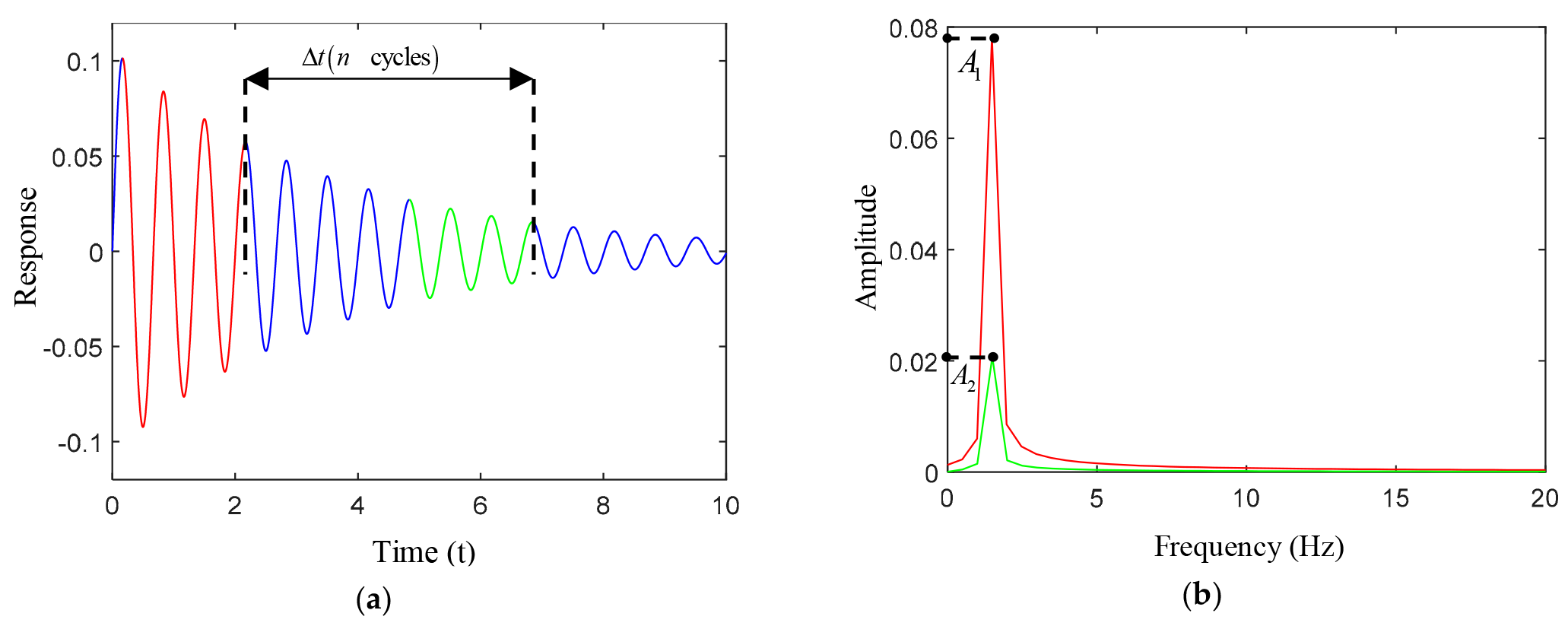
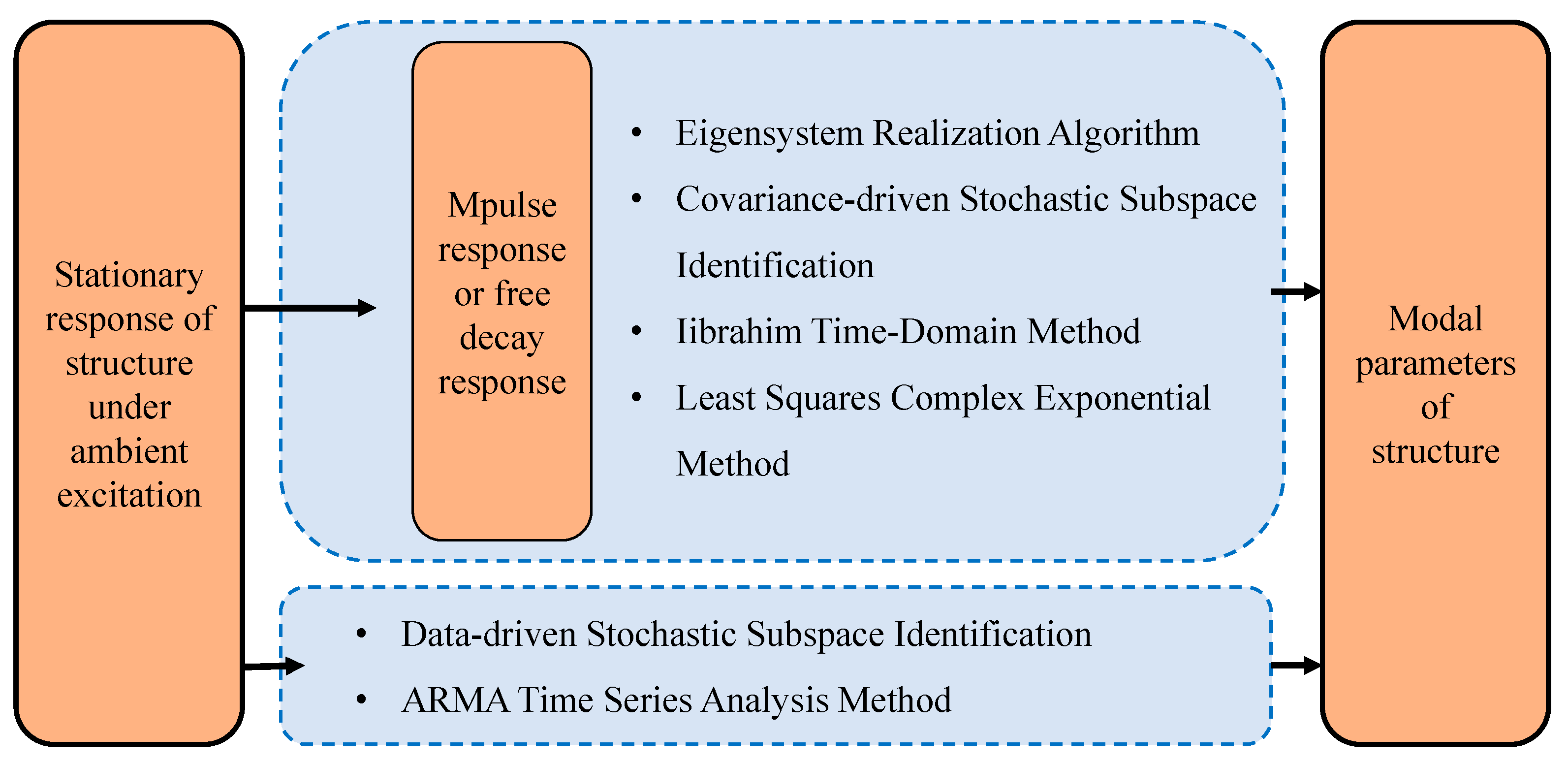
3.1.1. Time Domain Identification Method

Time domain identification methods directly use the time domain signals of structural responses for analysis and calculation, without the need for Fourier transformation, thus avoiding issues such as spectral leakage, sidelobe interference, and frequency resolution. In recent years, the most commonly used time domain identification methods in the field of civil engineering include the following:

• Logarithmic decrement method

The logarithmic attenuation method is the simplest and most commonly used time domain method for determining the viscous damping ratio through experiments. As shown in Figure 1, the basic principle of this method [42] is to calculate the modal damping ratio by measuring the amplitude ratio of the free attenuation response of a single-degree-of-freedom structure between two adjacent peaks, as shown in Equation (25). This is a method for calculating the damping ratio of single-degree-of-freedom structures, and the damping ratio identification accuracy of multi-degree-of-freedom structures is poor.

$$\xi ={\displaystyle \frac{v_n-v_{n+1}}{2\pi v_{n+1}}}$$

(25)

where $v_n$ is the nth peak of the damped free vibration response.

Shang et al. [43] proposed a method based on semantic segmentation of time series to extract the free decay segment from structural health monitoring (SHM) data, and successfully calculated the modal damping ratio of bridge structures using the logarithmic decrement method. This method based on time series semantic segmentation improves the applicability of the logarithmic attenuation method and makes it suitable for bridge health monitoring data. However, this method has high requirements for the quality of monitoring data, and the recognition accuracy is highly dependent on the quality of model training. Magalhaes et al. [44] compared the quality of the modal damping ratio based on the free vibration test and environmental vibration test, and the results show that the free vibration test can obtain more accurate damping ratio estimation. The short-term estimation of environmental vibration test time has high discreteness, and the long test time has the influence of aerodynamic damping, so the applicability of the above method based on time series semantic segmentation is further verified. For the damping ratio of a multi-degree-of-freedom structure, the spectral component of a certain mode is usually retained by band-pass filtering in the frequency domain and then converted to the time domain for calculation. For this problem, Lamarque et al. [45] studied a new method based on wavelet analysis to identify the damping of multi-degree-of-freedom systems. Compared with the traditional logarithmic decrement formula, the new method provides higher accuracy and better noise resistance in estimating the modal damping ratio. López-Aragón et al. [46] proposed a spectrum reduction method in the frequency domain instead of the logarithmic attenuation method in the time domain, as shown in Figure 2. The core idea is to intercept different intervals of the same free decay response and compare the amplitude reduction of the spectrum in two different intervals to calculate the modal damping ratio, as shown in Equation (26). This method can more clearly separate the contribution of each mode, making it more accurate to estimate the damping ratio of a specific mode in a multi-degree-of-freedom system. Frequency domain analysis usually has better robustness to noise, thereby reducing the impact of noise. The proposed method is applied to the modal parameter identification of the Arkonetal arch bridge and compared with the stochastic subspace method to ensure the feasibility of the proposed method.

$$\xi ={\displaystyle \frac{\ln \left(A_1/A_2\right)}{2\pi f\Delta t}}$$

(26)

where $A_1$ and $A_2$ are the spectral amplitudes corresponding to the selected time domain response, respectively. $f$ is the frequency of the response. $\Delta t$ is the time interval of the selected response.

2.

Eigensystem realization algorithm (ERA)

The eigensystem realization algorithm (ERA) uses the impulse response function of the multi-input multi-output system as its fundamental model. By constructing a generalized Hankel matrix, it employs singular value decomposition to derive the system matrix of minimum order, from which modal parameters are then extracted. The algorithm has rigorous theoretical derivation and recognition accuracy and has been widely applied in parameter identification under environmental excitation. By using singular value decomposition to obtain the system matrix, ERA can reduce the influence of noise on the results to a certain extent and improve the robustness and accuracy of the model. However, with the increase in the order of the system, the computational complexity and the time required will increase significantly. When multiple modes in the system are very close, modal aliasing is prone to occur, which affects the accuracy of parameter estimation.

The natural excitation technique (NExT) reveals that, under white noise excitation, the ratio of the autocorrelation function to the cross-correlation function of the response between two points of the structure is consistent with the impulse response function. This ratio can be used to replace the impulse response function, thereby allowing the ERA method to be conveniently used for identifying the modal parameters of the structure. Siringoringo et al. [47] used NExT-ERA to analyze the environmental vibration response of a suspension bridge and identified the first nine vertical bending modal damping ratios of the bridge. Compared with the Ibrahim time domain method, ERA shows higher efficiency in processing large-scale measurement data. Due to noise and calculation errors, the ERA algorithm will inevitably introduce false modes. In order to solve this problem, Zhang et al. [48] introduced the modal similarity index (MSI) and the modal energy level (MEL) to establish a hierarchical clustering technique to realize the automatic analysis method of the stability diagram of the ERA algorithm and used it to estimate the modal damping ratio of the Chaotianmen Bridge model. The damping ratio calculated by the multi-reference least squares complex frequency domain method is completely consistent, which verifies the effectiveness of the proposed method. The nonlinear relationship between eigenvalues and damping parameters of non-viscous damping systems proposed by Shen et al. [49] extended the improved eigensystem realization algorithm for modal parameter identification and relaxation parameters, from viscous damping systems to non-viscous damping systems. He et al. [50] took a suspension bridge as the research object and found that the bridge modal damping ratio identified by the NExT-ERA method with multiple reference points had great discreteness because the environmental excitation did not fully meet the broadband hypothesis and amplitude stability. Qu et al. [51] proposed a modal parameter identification method based on the combination of virtual frequency response function (VFRF) and ERA, considering that the actual engineering conditions often do not satisfy the assumption that the excitation is a stationary white noise, which improves the limitation of NExT-ERA technology to a certain extent.

At present, the ERA method is mainly applied to linear systems, and there are still some limitations to the identification of complex nonlinear systems. In the future, the relationship between eigenvalues and modal parameters of nonlinear systems can be further studied, and the ERA method suitable for complex nonlinear systems can be developed.

3.

Stochastic subspace identification (SSI)

The stochastic subspace identification (SSI) algorithm can be divided into covariance-driven stochastic subspace method and data-driven stochastic subspace method according to the way of processing and analyzing measurement data. The covariance-driven stochastic subspace method uses the random response covariance matrix of the structure to construct a Toeplitz matrix and then obtains the system state matrix through singular value decomposition, ultimately calculating the structural modal parameters. The data-driven stochastic subspace method constructs a Hankel matrix from measured data and obtains the observation matrix and state sequence of the system via QR decomposition. Finally, the system matrix of the structure is calculated using the least squares method, and the modal parameters of the structure are determined. This method exhibits strong anti-noise performance and can accurately identify the frequency, vibration modes, and modal damping ratios of the structure. This method has many advantages: modal parameter identification can be completed without input signal; it has strong anti-noise ability and can effectively identify the modal parameters of the structure from the noisy data. It has a wide range of applications, not only for linear systems but also for the analysis of nonlinear systems. The whole process can be highly automated. However, its computational complexity is high. In order to ensure the accuracy of the recognition results, a large amount of test data are needed. However, it is vulnerable to the interference of false modes.

Ozcelik et al. [52] used a data-driven SSI algorithm to identify three environmental vibration tests at different temperatures on a 199 + 325 m steel highway bridge in Usak, Turkey, and compared the identification results with the enhanced frequency domain decomposition method. The results show that the estimated damping ratio shows a high degree of variability. Lorenzoni et al. [53] used the SSI algorithm to identify the monitoring data of a multi-span reinforced concrete beam bridge for a total of 12 months and found that the modal damping estimation results had higher scattering than the natural frequency. Zabel et al. [54] extracted the first 12 modes of a concrete railway bridge by using the cooperative anti-difference driving SSI algorithm. Compared with the modal damping ratio estimated by the logarithmic attenuation method, the identified values of some modal damping ratios are larger. According to the difference in response data processing methods, the stochastic subspace identification method is divided into data-driven and covariance-driven stochastic subspace identification methods. Traditionally, these two methods are considered to be consistent in theory and practice. Xin et al. [55] studied these two different data processing methods and found that the limited amount of data will lead to a deviation between the estimated value and the true value. QR decomposition will also affect the estimation results in the parameter estimation process.

By summarizing the above literature, it is found that for all bridges, the estimation of natural frequency is more accurate and the standard deviation is lower. However, the estimation of modal damping is affected by many uncertain factors. The identification of modal damping ratio is affected by structural type, length of acquisition time, environmental noise, loading and environmental effects.

4.

Ibrahim time domain method (ITD)

The ITD identification method was proposed by Ibrahim in the 1970s. This technique was originally based on impulse response functions or general free decay for single-input multi-output modal analysis. The basic principle of this method is to construct two response matrices with specific time delay by using free vibration response data, and form an eigenvalue problem (EVP) through the delay relationship between the two matrices, and then solve the natural frequency, damping ratio and modal shape. Modal parameters such as mode shape. However, this method has problems in dealing with closely spaced modes, so it has not been widely used in the past few decades. The ITD method mainly depends on the free vibration response data, so it is very sensitive to noise and vulnerable to environmental interference. Moreover, this method has high computational complexity and a large amount of calculation in the process of constructing and solving eigenvalue problems.

After a long period of development, Brincker et al. [56] studied a more modern ITD technology, by adding a Toeplitz matrix to deal with a set of free attenuation, so as to realize the processing of multi-input data. The results show that this technology can effectively deal with the closely spaced modes. Tian et al. [57] obtained the free response signal of velocity by random decrement technique and then identified the modal parameters by the ITD method through the velocity signal. Anuar et al. [58] successfully identified the natural frequency of the steel plate structure by ITD identification method. Cárdenas et al. [59] compared the enhanced frequency domain decomposition method (EFDD) with the ITD identification method. The results showed that the ITD method could not identify all the modes. Due to the influence of spectral leakage, the damping ratio identified by the enhanced frequency domain decomposition method showed a large variability. The influence of different numbers of accelerometers and different excitation conditions on modal parameter identification is also considered in the study.

There are solutions to the limitations of the ITD identification method in dealing with closely spaced modes, but it is still difficult to solve the problems of environmental noise and complex calculation processes.

5.

ARMA time series model analysis method

ARMA model is a linear model widely used in time series analysis. It can be used to identify the modal parameters of the structure, which is usually used in the field of mechanical engineering. This method realizes modal parameter identification by converting the excitation and response expressed by high-order differential equations into time series difference equations based on different time points. The ARMA model consists of an autoregressive (AR) part and a moving average (MA) part, which can be expressed as a linear combination of past values and random perturbations. The ARMA model can use a limited amount of data, and the frequency transfer function obtained from the time series model can avoid the rounding error, so it has a wide range of application prospects.

Pi et al. [60] used the autoregressive moving average (ARMA) model of vibrating structures to identify modal parameters. The relationship between the structural autoregressive (AR) model and the moving average (MA) model is derived. The coefficient matrix sequence of the AR model is estimated by using the excitation and response data, and then the impulse response function matrix sequence of the structure is calculated by the relationship between the AR and MA models. The estimated impulse response function matrix and poles are used to identify the modal parameters of the structure. Pei et al. [61] simulated the acceleration response of a three-story reinforced concrete frame structure model under white noise excitation and identified modal parameters by the ARMA time series analysis method. The research shows that this method can effectively identify modal parameters. Its frequency identification accuracy is high and anti-noise ability is strong, but the accuracy in identifying modal damping ratio is low, especially for high-order modal damping ratio. Chen et al. [62] introduced a modal parameter estimation technique based on the random decrement de-noising autoregressive moving average (RDT-ARMA) method. The random decrement method is used to eliminate the noise in the free response, so as to obtain a more realistic free response signal. Then, the ARMA method is used to identify the modal parameters.

The ARMA time series method has high accuracy in frequency identification and can effectively resist the influence of noise, but the identification accuracy of the damping ratio is relatively low, especially for the high-order damping ratio. Order selection is an important research direction, and improper order selection may affect the accuracy and stability of the model.

6.

Least squares complex exponential (LSCE)

The least squares complex exponential method (LSCE) expresses the free vibration response of the system as a linear combination of a series of complex exponential functions. The free vibration response data of the system are processed by least squares fitting to extract modal parameters, such as modal frequency, modal damping ratio, and vibration mode. This method is especially suitable for modal identification of multi-mode and multi-degree-of-freedom systems.

Chen et al. [63] compared the least squares complex exponential method and the eigensystem realization algorithm (ERA) through the experiment of a cantilever beam and found that the recognition accuracy of ERA in a noisy environment is due to LSCE. Argentini et al. [64] compared the LSCE and frequency domain decomposition modal identification methods through the actual monitoring data of cable-stayed bridges and found that the combination of the LSCE method and random decrement technique can effectively identify the modal parameters of cable-stayed bridges. There are some differences between the modal damping ratios determined by the LSCE method and the FDD method. The difference may be due to the different data processing methods and the different principles and assumptions of the identification methods.

7.

Empirical Mode Decomposition (EMD)

Empirical mode decomposition (EMD) is a signal processing method used to decompose complex signals into a set of simple oscillation modes called intrinsic mode functions (IMF). The EMD method was originally proposed by Huang et al. [65] in 1998 to deal with non-linear and non-stationary signals. Since the measured vibration data are often multi-modal, the empirical mode decomposition technique can be used to decompose the multi-modal data into a series of quasi-single-modal intrinsic mode functions (IMFs). Then, ERA, SSI, ITD and other time domain methods can be used to identify modal parameters more conveniently and reduce the generation of false modes. The EMD method also has a good denoising effect. Bekara et al. [66] used empirical mode decomposition to remove random noise and coherent noise in seismic data and studied the surface denoising effect.

The traditional EMD method may encounter the problem of modal aliasing when dealing with actual signals, that is, an IMF contains components of different frequencies, as well as endpoint effects. In order to solve these problems, Huang et al. [67] proposed the EEMD method. The basic idea of EEMD is to add a series of white noise to the original signal, perform EMD decomposition on each group of noisy signals, and then average the results of all IMFs to obtain the final IMF component. Through this method, white noise can fill the missing part of the information in the signal, making the decomposition result more stable and reliable, and reducing the mode mixing phenomenon. Wang et al. [68] compared the effects of EMD and EEMD in processing signals and determined that EEMD can solve the problem of modal aliasing. Torres et al. [69] found that there is residual noise in the EEMD reconstructed signal, and different implementations may produce different numbers of IMFs. They proposed to add specific noise at each stage of decomposition, calculate the only residual to obtain each mode, and finally obtain a complete decomposition. The proposed new method reduces the number of iterations on the basis of solving modal aliasing.

From the development process of the EMD method, it can be seen that EMD and its derivative methods have always focused on improving the accuracy and stability of signal decomposition from the initial proposal to the subsequent continuous improvement and improvement. The development of these techniques has greatly promoted the development of nonlinear and non-stationary signal analysis and provided a powerful tool for the study of modal parameter identification.

8.

Recursive digital technique (RDT)

Recursive digital technique (RDT) is a recursive digital filtering technique that is mainly used for modal analysis and feature extraction in signal processing. By iteratively extracting different modal components in the signal, RDT performs well in dealing with nonlinear signals and is widely used in structural dynamics and vibration signal processing. Like EMD, it is also a signal processing method.

Feng et al. [70] proposed a consistent multi-level RDT-ERA method, using multiple trigger levels, and proposed to use consistency analysis to eliminate the identification results with large deviations from most trigger levels. Finally, the weighted average method is used to calculate the final estimation of modal parameters. Feng et al. [71] proposed an enhancement method based on the empirical mode decomposition–random decrement technique (EMD-RDT) for operational modal analysis, which has the advantage of separating the vibration mode and modal coordinates from the free decay modal response, thereby improving the efficiency of the identification process. He et al. [72] proposed a bridge modal parameter identification method combining EMD and RDT. By minimizing the error between the predicted free decay response and the measured free decay response, the natural frequency and the Yang’s ratio were calculated and the method was applied to the Nanjing Yangtze River Bridge.

With the increase in structural complexity, the computational efficiency of the random decrement technique (RDT) in modal parameter identification is becoming more and more prominent. Future research needs to further optimize the algorithm to reduce the computational time and resource consumption. In practical applications, the measurement data is often affected by noise and interference. Therefore, it is also an important development direction to improve the robustness of RDT so that it can work stably under various harsh conditions.

The first six of the above eight methods are used for modal parameter identification. The latter two methods are signal processing methods, which are only used to decompose multi-modal vibration signals into single-modal vibration signals or noise in out-of-response. The purpose is to preprocess the required signals for the first six modal identification methods. The time domain identification method can be divided into a one-step method and a two-step method, as shown in Figure 3. The one-step method is used to obtain the modal parameters directly from the response signal. The two-step method needs to calculate the approximate free attenuation signal through the response signal and then identify the modal parameters.

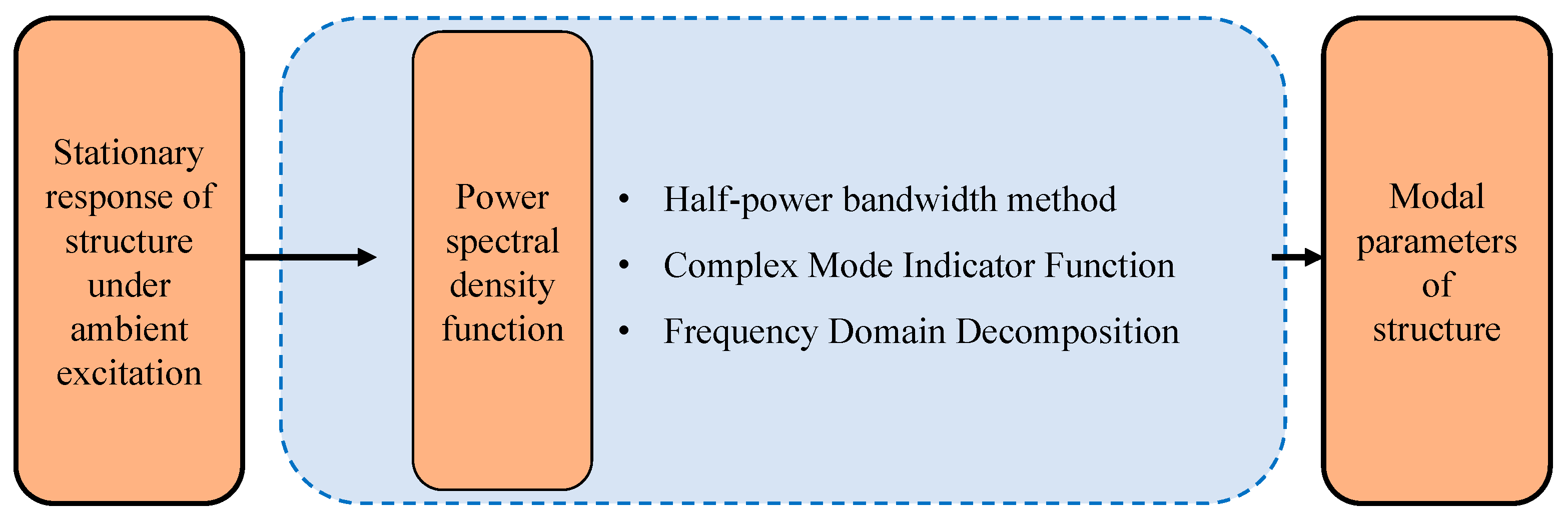
3.1.2. Frequency Domain Identification Method

In the operation modal analysis, the advantage of the frequency domain identification method is that the spectrum characteristics are intuitive and the modal distribution is clear. In the process of calculating the spectrum, the average technology is used for a long time to minimize the noise interference, so that the modal order problem can be solved. However, the spectrum quality directly affects the accuracy of modal parameter identification, so it is necessary to use high-precision sensors and sufficient sampling frequency and sampling time. At present, the most commonly used frequency domain identification methods in the field of civil engineering mainly include the following:

• Half-power bandwidth method

The half-power bandwidth method [73] is the simplest method for the tester to estimate the modal damping. The calculation principle is to solve the modal damping ratio by the ratio of the frequency difference corresponding to the left and right half power points of the frequency response function to the peak point frequency, as shown in Equation (27). This method is simple and intuitive, and the calculation process is convenient, as shown in Figure 4, but it cannot identify dense modes [74]. When the modal damping ratio is greater than 38.5%, this method will no longer be applicable. At the same time, the selection of the peak value of the natural frequency requires a multi-point spectrum comparison [75], which cannot effectively distinguish the real mode and the noise mode.

$$\xi ={\displaystyle \frac{{\omega }_2-{\omega }_1}{2{\omega }_0}}$$

(27)

where ${\omega }_1$ and ${\omega }_2$ are the frequencies corresponding to the left and right half power points, respectively; ${\omega }_0$ is the modal natural frequency.

Brownjohn et al. [76] windowed the acceleration spectrum of the Humber Bridge under ambient excitation and used this method to identify the modal damping ratio. It is considered that the damping decreases with the increase in frequency, and the estimated value of damping is too large. For the approximate calculation of the half-power bandwidth method, Wu et al. [77] proposed a third-order correction formula. The numerical simulation shows that the third-order correction formula effectively improves the recognition accuracy. Papagiannopoulos et al. [78] used the third-order correction formula to identify the modal damping ratio of a three-story building structure and verified the reliability of the third-order correction formula. At the same time, it was found that the identification error of the modal damping ratio of high-order modes was large. Olmos et al. [79] studied the applicability of the half-power bandwidth method to non-real modes. The results show that the half-power bandwidth method is also applicable to the modal damping ratio estimation of non-real modal systems.

The half-power bandwidth method is an approximate method. The calculated damping ratio is not an accurate solution. The third-order correction formula only improves the calculation accuracy and is not an accurate solution. The identification accuracy is lower when there are frequency domain problems such as spectrum leakage and spectrum aliasing. Moreover, the half-power bandwidth method can only calculate the damping ratio of a certain mode alone and inevitably receives the influence of other modes.

2.

Complex mode indicator function (CMIF)

The complex mode indicator function method [80] (CMIF) is the singular value decomposition of the measured frequency response function matrix corresponding to each discrete frequency point, and the number of peaks of the maximum singular value curve is used to determine the structural mode order, that is, the peak value of the singular value curve corresponds to the natural frequency of the structure, and the first left singular vector corresponding to each order frequency is the mode shape. For the modal damping ratio and modal scaling factor, the method uses the weakening orthogonality of each mode to decouple the measured frequency response matrix through the singular vector to form an enhanced frequency response function in the form of a single degree of freedom [81], and then uses the polynomial fitting method to identify the structural modal damping ratio. Therefore, this method requires that the arrangement of the measuring points should have good mode orthogonality, and in order to ensure the identification accuracy of the low-order modal parameters, the frequency resolution of the measured data is very high.

Tian et al. [82] carried out a multi-reference point impact test on a three-span concrete box girder and used CMIF to obtain modal parameters such as structural modal damping ratio, so as to predict structural deflection under arbitrary load. Gul et al. [83] conducted an environmental vibration test on a two-span bridge benchmark model. Based on the combination of CMIF and the random decrement method, the unscaled frequency response function was obtained from the output data set to identify the damping ratio. Compared with the modal damping ratio identification results of the impact test, the accuracy of the identification results was verified. Lin [84] proposed a complex modal indicator function based on singular value decomposition to identify structural systems with severe adjacent modes, which overcomes the difficulties of traditional modal identification techniques in dealing with closely distributed modes and non-classical damping structures, making the estimation of modal parameters more accurate and reliable. Bakir et al. [85] applied the complex modal indicator function method to the modal analysis of a building in a university in Turkey and compared it with the results of the stochastic subspace identification method. It was found that the CMIF technique can identify the modal shape most clearly, and the system identification technique based on stochastic subspace can better estimate the damping ratio.

The complex modal indicator function method shows high accuracy, strong robustness and wide adaptability in modal parameter identification, especially for structures with closely distributed modes and non-classical damping characteristics. However, this method has high computational complexity, strict requirements on the quality of measured data, and certain limitations in high-frequency modal parameter identification.

3.

Frequency domain decomposition (FDD)

Based on the peak picking method (PP) [86], Brincker proposed the frequency domain decomposition (FDD) [87]. This method is similar to the complex modal indicator function method, which can perform singular value decomposition on the frequency response function matrix or power spectral density matrix to obtain the frequency and mode shape of the structure. In order to obtain more accurate damping estimation results, it has gradually developed into an enhanced frequency domain decomposition method, that is, the single-degree-of-freedom attenuation curve is obtained by inverse Fourier transform of the frequency response data near the peak frequency of each order, and the structural modal damping ratio is identified by logarithmic attenuation method. This method can identify dense modes and has a strong anti-noise ability, which is suitable for operational modal analysis. However, in the process of modal damping ratio identification, it is converted from the frequency domain to the time domain, resulting in the loss of identification accuracy.

Ghalishooyan et al. [88] proposed an operational modal assignment algorithm to improve the identification program of modal frequency and modal damping ratio in the enhanced frequency domain decomposition method. According to the identification results of a four-story frame under random excitation, it is verified that the calculation error and deviation of the modal damping ratio of all vibration modes are significantly reduced. In order to make up for the deficiency of the frequency domain decomposition method in identifying the accuracy of the modal damping ratio, Qu et al. [89] proposed an iterative frequency domain decomposition method. The natural frequency and modal shape obtained by FDD are substituted into the output power spectrum formula to construct nonlinear equations, and then the iterative optimization method is used to solve these equations to obtain the modal damping ratio. Numerical examples verify the effectiveness of the method. When the two-order modal interval is close or the modal damping ratio is large, the frequency domain decomposition method cannot accurately identify the modal damping ratio, and the noise has a great influence on the FDD. In order to solve this problem, Brincker et al. [90] proposed an enhanced frequency domain decomposition method combined with time domain analysis. Hasan et al. [91] found that EFDD underestimates the damping of high damping systems and is affected by spectrum leakage and spectrum aliasing. In the structural vibration test, in order to reduce the influence of environmental noise, the response data is usually truncated. However, this approach will lead to spectrum leakage errors. In order to solve the leakage error caused by truncation, Qu et al. [92] derived the expression of spectrum leakage error from frequency response function and free attenuation data and applied it to FDD to compensate for spectrum leakage error by iterative method. The effectiveness of the method is verified by a four-layer frame benchmark model.

FDD and its variants perform well in operational modal analysis due to their wide application range, good anti-noise ability and easy implementation, especially for structural health monitoring under complex environmental conditions. However, when dealing with modal-intensive or high-damping systems, the accuracy of damping ratio identification is low. When the method also faces spectrum leakage and aliasing problems, these factors will significantly affect the final modal parameter identification results.

The frequency domain method needs to perform a Fourier transform on the response signal to obtain the frequency response function or power spectral density function, and then identify the modal parameters, as shown in Figure 5. The key problem of using the frequency domain method to identify structural modal parameters is the quality of the measured frequency response data. The measured frequency response data with good quality should meet the two conditions of ‘smooth’ and ‘full’. ‘Smooth’ means that the frequency response data is less disturbed by random environmental noise, the signal-to-noise ratio is high, and the curve is relatively smooth; fullness means that the measured frequency response function satisfies a certain frequency resolution, and there are enough data points near each mode to ensure the accuracy of modal parameter identification.

3.1.3. Time-Frequency Domain Identification Method

• Wavelet analysis (WA)

Wavelet analysis (WA) is a powerful tool in modal parameter identification, which is used to deal with non-stationary signals and multi-resolution analysis. Wavelet analysis can provide both time domain and frequency domain information, which is very useful for analyzing transient signals and capturing local features of signals. In the modal parameter identification, the core idea is to use the free vibration response of the structure or the intrinsic mode function (IMF) after the modal decomposition of the free vibration response of the structure. Based on the mapping relationship between the modal parameters and the signal distribution characteristics (amplitude, phase angle), the modal parameters such as the natural frequency and modal damping ratio of the structure are obtained by means of least square fitting and half power bandwidth.

Wavelet analysis was first proposed by Morlet in 1982 [93]. However, there is still a boundary effect problem in wavelet transform. Kijewski et al. [94] analyzed the boundary effect problem in detail and proposed to add data at the end to reduce the influence of boundary effect. By minimizing the wavelet transform entropy, Lardies et al. [95] obtained an improved sub-wavelet function form of time and frequency resolution, and proved that the natural frequency and modal damping ratio of the system can be estimated by the wavelet transform of the free response of the system. Traditional wavelet transform requires predefined wavelet basis functions. The selection of these basis functions is often fixed and may not always be the most suitable for all types of signals. For these problems, Gilles [96] proposed empirical wavelet transform (EWT), which is a new method for signal processing. EWT can effectively analyze non-stationary signals in the time and frequency domain by adaptively dividing the frequency band and extracting the corresponding wavelet according to the characteristics of the signal.

2.

Hilbert–Huang transform (HHT)

Hilbert–Huang transform (HHT) is a powerful tool for analyzing nonlinear and non-stationary signals. It is an adaptive processing method for analyzing nonlinear and non-stationary signals proposed by Huang in 1998 [65]. HHT combines empirical mode decomposition (EMD) and Hilbert transform, which can be used to extract the time-frequency characteristics of the signal and identify modal parameters such as natural frequency, modal damping ratio and vibration mode. Yan et al. [97] compared the effect of wavelet transform and Hilbert–Huang transform in signal processing and found that the Hilbert–Huang transform makes it difficult to separate dense modes, and both methods are affected by the end effect.

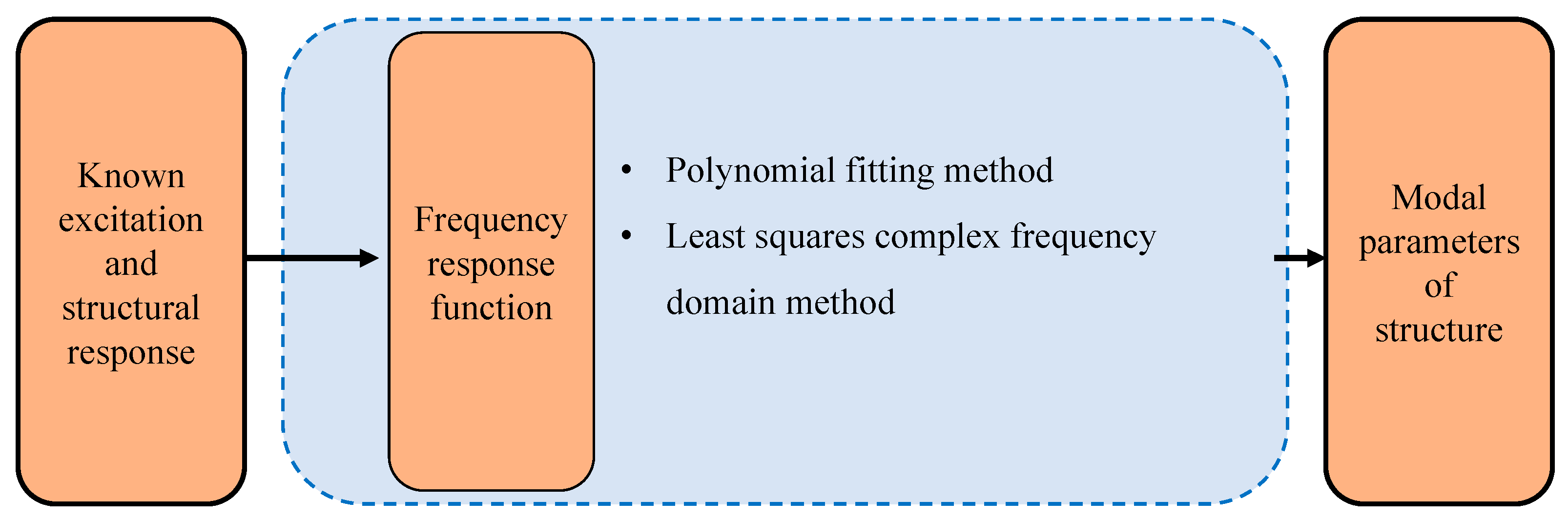
3.2. Modal Damping Ratio Identification of Bridge Structure Based on Response Under Artificial Excitation

The bridge modal damping ratio identified by operational modal analysis is very discrete because the environmental excitation does not fully meet the broadband assumption and amplitude stability. Compared with the artificial excitation of environmental excitation, the response data with a larger amplitude and higher signal-to-noise ratio can be obtained, and there is no assumption that the excitation is white noise, so the identified modal damping ratio is more accurate. The modal parameters of the bridge are identified based on the dynamic response signal generated by the artificial excitation method, which can be roughly divided into two categories: the known excitation method and the free vibration method. The known excitation method is used to measure the excitation data and response data by means of exciter, hammer and so on. The modal damping ratio is calculated by the half-power bandwidth method or the logarithmic attenuation method for the free attenuation signal generated by excitation methods such as sudden loading, sudden release, and jumping. This method is called the free vibration method. The method of identifying the damping ratio of bridge structure by free vibration response is the same as the method of identifying the damping ratio of bridge structure based on environmental excitation. When the excitation is known, the frequency response function of the structure can be calculated, and then the damping ratio of the bridge structure can be identified by fitting the frequency response function.

3.2.1. Polynomial Fitting Method

The earliest polynomial fitting method was the rational fractional polynomial method (RFP) proposed by Levy [98]. This method uses power polynomials as basis functions and fits the measured frequency response curve using a rational fractional mathematical model. Due to the precision of the theoretical model, it achieves high identification accuracy; however, solving high-order coefficient matrices results in ill-conditioned equations, reducing numerical stability. To address this issue, Richardson [99] proposed the orthogonal polynomial method for modal parameter identification, decoupling the coefficient matrix using Forsythe complex orthogonal polynomials [100], reducing the order of the equation system and enhancing computational stability. Arruda et al. [101] introduced the concept of minimizing the correlation coefficient between two curves as an objective function and demonstrated an iterative process where each step includes a least squares nonlinear fit with scaled curves, emphasizing the importance of selecting the objective function. Duan et al. [102] studied the weighted fitting of frequency response functions, defining an objective function to minimize the difference between measured and computed frequency response functions, and identified the modal frequencies and damping of the structure through a weighted fitting process.

The main principle of the polynomial fitting method is to obtain the modal parameters by fitting the measured frequency response function through the model. The models of the existing fitting methods are all ideal frequency response functions, but the actual frequency response functions measured by experiments do not conform to the model due to spectrum leakage and spectrum aliasing. Therefore, the next development direction should be to calculate the model under different sampling times and different sampling frequencies and define different models for different situations so as to accurately identify the modal damping ratio.

3.2.2. Least Square Complex Frequency Domain (LSCF)

The least square complex frequency domain method (LSCF) uses the common denominator matrix model in the z domain to fit the frequency response curve. The matrix coefficients are calculated by the compressed canonical equation and the right matrix is constructed on the basis of the matrix coefficients. The eigenvalue decomposition of the right matrix is carried out to obtain the frequency, damping and modal participation factors of the structure. Then, the least squares estimation of the frequency response function equations is used to obtain the vibration mode. In order to improve the identification ability of structural dense modes, Peeters [103] used the right matrix fractional model to replace the common denominator model and extended the least squares complex frequency domain method to the multi-reference point form, and finally formed the multi-reference point least squares complex frequency domain method. This method can also form a clear stability diagram under the condition of low signal-to-noise ratio and can identify the structural modal parameters in the wide frequency band at one time. It has good parameter identification results for strong damping and weak damping structures.

Brown John et al. [104] performed low-pass filtering on the acceleration response of the Humber Bridge to obtain a spectrum within 0~1 Hz. At the same time, the response data of different sections are combined to enhance the contribution of different types of modes in the power spectrum, and then the modal damping ratio of the first 12 bending modes is identified by the least square complex frequency domain method. The generalized total least squares (GTLS) algorithm proposed by Verboven et al. [105] achieves accurate modal parameter estimation by integrating the noise model into the parameter identification process. A new frequency-domain data merging method is proposed by Hızal [106]. The least square method is used to fuse multiple sets of measurement data in the pre-identification stage, which improves the quality of modal parameter estimation in operational modal analysis.

Similar to the polynomial fitting method, the least squares complex frequency domain method also extracts the modal parameters of the system from the fitting data by fitting the measured frequency response function. Therefore, the two have the same problem, that is, the fitting model is different from the measured frequency response function.

The above two frequency domain methods are used to identify the damping ratio of the bridge structure by fitting the frequency response function, and the calculation process is shown in Figure 6.

According to the number of input excitation points and output response points, the experimental modal analysis method can be divided into the single-input single-output (SISO) method [107], the single-input multiple-output (SIMO) method [56] and the multipleinput multiple-output (MIMO) method [108]. Among them, the single-input single-output method can only identify the natural frequency and modal damping ratio of the structure. Based on the requirements of identifying structural vibration modes, the single-input multi-output method and the multi-input multi-output method are generally used in practical engineering.

The SIMO method is adopted, which causes the input energy to be concentrated at one point. The amplitude of the measuring point near the excitation point is large, and the amplitude away from the excitation point is small, which will affect the accuracy of modal parameter identification. Moreover, only one row or one column of the frequency response function matrix can be obtained by using the single input multiple output method, which will also affect the recognition accuracy. Based on the above reasons, the SIMO method still has many limitations in the modal parameter identification of large and complex structures. In the SIMO method, the frequency response function of all measuring points is used to identify the modal damping and natural frequency. The core is the rational fraction orthogonal polynomial fitting method. According to the modal information such as frequency and damping ratio contained in the frequency response function, the modal parameters such as natural frequency and damping ratio are obtained by using the least squares principle.

In order to solve the disadvantages of the SIMO method, the MIMO method came into being. The core idea is to use several column frequency response functions obtained by multiple excitation points to identify the modal parameters. Its advantage is that the excitation energy distribution is uniform, the response signal-to-noise ratio of each measuring point is high, and the frequency response function matrix is used to identify the modal parameters with higher accuracy. The specific method of identifying modal parameters based on multi-input multi-output method is basically the same as that of operational modal analysis, and there are only differences in the assumption of input load.

3.3. Abnormal Data Processing and Modal Verification

3.3.1. Abnormal Data Processing

In recent years, with the rapid development of machine learning technology, it has shown great potential and value in solving the problem of structural modal parameter identification, which has brought a new perspective to the research of this traditional field. A convolutional neural network is a typical representative algorithm of deep learning. Its internal complex training mechanism can capture the nonlinear relationship and multi-modal distribution in the data and has good anomaly detection accuracy [109]. In recent years, when using a convolutional neural network for anomaly detection of structural health monitoring data, anomaly detection is often realized by converting time series data into image form and then using a convolutional neural network model for recognition and classification, as shown in Figure 7. When using the convolutional neural network model for recognition and classification to achieve anomaly detection, only the response data need to be converted into images for analysis, and the x-axis and y-axis do not need to be drawn. This method can make full use of the powerful image recognition ability of the convolutional neural network to better capture and learn the spatial patterns in the data and quickly realize automatic detection of large-scale data.

Lee et al. [110] converted acceleration data into images based on railway bridge data to train the convolutional neural network model to achieve data detection. Kim et al. [111] used convolutional neural networks to perform anomaly detection on multi-category imbalanced data. Before training, the data set was balanced by data supplementation, and the balanced data set achieved an overall accuracy of 97.6%. Zhang et al. [112] combined the convolutional neural network with the long-term and short-term memory network and used the time domain and frequency-domain dual-channel images converted from the original data to train the combined model to realize the anomaly detection of vibration data. Jana et al. [113] proposed a deep learning framework for anomaly detection and reconstruction of sensor signals. First, convolutional neural networks are used to detect the presence of faults and identify their types. Next, a set of individually trained convolutional autoencoder networks corresponding to each type of fault is used for data reconstruction.

3.3.2. Modal Verification

Modal verification or false modal elimination is an indispensable part of the field of modal identification, especially in dealing with modal identification under environmental excitation. In such scenarios, due to the difficulty in obtaining complete excitation and response data to construct the model, coupled with the influence of factors such as noise interference and insufficient excitation, the accuracy and accuracy of modal identification results are challenged, which in turn affects the robustness of the algorithm. In view of this, after the completion of modal identification, the use of effective modal verification methods to rigorously identify the identification results has become crucial. Modal verification methods mainly include two types, mathematical index verification and stability diagram verification. The verification of mathematical indicators focuses on quantitative analysis. By calculating specific mathematical indicators, the rationality of modal parameters is evaluated, such as coherence function and residual analysis. This method can provide more objective data support. Stability diagram (SD) is a commonly used system pole identification method based on system order sensitivity analysis. In view of the close relationship between modal parameters and system poles, this method can effectively improve the accuracy of verification.

• Mathematical indication verification method

At present, the commonly used mathematical index verification methods play an important role in modal verification. These methods can evaluate the reliability and accuracy of modal parameters from different angles. The following are several main mathematical index verification methods and their applications:

(1)

Modal assurance criterion (MAC)

MAC is an index used to measure the correlation between different modal shapes. It is usually used to match the calculated mode with the experimental mode and is often used to eliminate false modes or to compare the modal shapes of damaged and undamaged states to determine the degree of damage. In the modal verification, the autocorrelation and cross-correlation analysis of MAC can be carried out by using different order modes, and the histogram is drawn for observation, as shown in Figure 8. The matrix expression of MAC is as follows:

$$\mathrm{MAC}({\varphi }_i,{\varphi }_j)={\displaystyle \frac{\left({\varphi }_i^H{\varphi }_j\right)\left({\varphi }_j^H{\varphi }_i\right)}{\left({\varphi }_i^H{\varphi }_i\right)\left({\varphi }_j^H{\varphi }_j\right)}}$$

(28)

where ${\varphi }_i$ and ${\varphi }_j$ represent the $i$ and $j$ mode shapes, respectively. ${\left(•\right)}^H$ represents the conjugate transpose.

The MAC estimate is affected by the uncertainty derived from the mode shape estimate. The uncertainty of MAC is mainly due to the modal shapes estimated from the measured data. These estimates are limited by data length, ambient noise and unknown excitation conditions, resulting in MAC not necessarily equal to 1 even if the modal shapes are theoretically the same. In practical applications, especially when the MAC value is close to 1, the traditional Gaussian distribution approximation cannot accurately describe its uncertainty because the MAC is limited to the [0, 1] interval. Therefore, accurately quantifying this uncertainty is particularly important for more accurate statistical inference. To solve this problem, Greś et al. [114] proposed two methods to deal with MAC uncertainty, which are suitable for MAC estimation in different situations. When the two modes have different shapes and the MAC value is between 0 and 1, the uncertainty of MAC can be approximated by Gaussian distribution, and the confidence interval can be quantified and calculated based on the first-order Taylor expansion. When the two modal shapes are the same, the MAC value is close to 1. At this time, the chi-square distribution approximation of scaling and offset is used, and the uncertainty is better quantified by the second-order Taylor expansion. The author applies these uncertainty quantification frameworks to the monitoring data of the S101 bridge, which proves that the method can detect early damage with constant frequency.

(2)

Mode Phase Collinearity (MPC)

The main function of MPC is to measure the complexity of the modal shape, which is between 0 and 1. When MPC = 1, the modal shape is a real-valued vector. When the MPC is small, the modal shape is more complex, which may be a false mode introduced by noise. Although MPC itself is not a tool specifically for eliminating spurious modes, its results can assist in the identification of spurious modes. In modal analysis, spurious modes are usually represented by unstable modal parameters, such as frequency, damping ratio, etc. These spurious modes may be caused by noise or calculation errors. MPC can be used to analyze the collinearity of modal shapes, helping to distinguish which modes are physically effective and which may be spurious modes caused by data noise or non-physical factors.

The data length has a significant effect on the uncertainty quantification of MPC. As the data length increases, the Gaussian distribution approximation of the MPC estimation gradually becomes more accurate, and especially when the MPC value is close to 1, more data are needed to ensure the rationality of the Gaussian approximation. The more data, the closer the MPC estimate is to its true value, meaning that the confidence interval will shrink and the results will be more stable and reliable. Greś et al. [115] studied the uncertainty quantification of MPC under complex modal shapes and proposed a framework based on Gaussian distribution approximation to evaluate the variance and confidence interval of MPC estimation. The effectiveness of the proposed method is verified by Monte Carlo simulation, and it is applied to the measured data of an offshore meteorological tower in the North Sea to eliminate the spurious modes caused by noise.

2.

Stabilization Diagram (SD)

In the modal analysis of bridge structure operation, due to the problems of noise interference or insufficient excitation, it is often not feasible to determine the order of the calculation system by the number of singular non-zero values of the matrix in the process of modal identification, so it is necessary to determine the setting before the identification begins. In practical engineering, the order of the system is often difficult to determine. In this regard, by setting a sufficiently high calculation system order, the incomplete recognition results can be solved. However, the number of identified results may increase with the increase in the calculation order, that is, more modes are introduced, which will include real modes and false modes. The stability diagram method is an effective method to determine the order of the system and can distinguish the true and false modes from many modes. The principle is to use different system orders to complete the modal identification, through the identification of the system pole. Figure 9 is a schematic diagram of the stable diagram method to eliminate false modes.

4. Summary and Outlook

Damping is one of the basic characteristics of bridge structure, which reflects the ability of bridge structure to dissipate energy during vibration. In the design and maintenance of bridges, the damping ratio has a direct impact on the safety and service life of the structure, thus affecting its sustainability. This paper comprehensively summarizes the damping models proposed by scholars at home and abroad, summarizes the progress of bridge structure damping ratio identification methods, and compares the advantages and disadvantages of operational modal analysis and experimental modal analysis. It is found that the damping ratio of the bridge structure is affected by many factors. The measured values of the damping ratio under different temperatures and different environmental conditions are quite different. Even if the conditions are the same, the damping ratios identified by different identification methods are still quite different. Based on the existing research results at home and abroad, future research should be carried out with the following five aspects in mind:

(1) The damping models of bridges with different structures are developed. Although there are many damping models at this stage, they still cannot accurately describe the energy dissipation of bridge structures. In view of the different bridge structures, there are many types of suspension bridges, e.g., cable-stayed bridges, beam bridges, arch bridges, etc., and the materials and components of bridges are becoming more and more complex. The existing damping models do not consider the mechanism of damping at the material and component levels, so there is a large error between the damping theoretical model and the actual bridge structure. The bridge should be decomposed into many components, each of which is described by an appropriate damping model. Finally, the damping matrix of the whole bridge is synthesized to identify the damping ratio. Future research should build a comprehensive damping ratio database based on different types of bridge structures, develop a model to describe the damping of each component of the bridge structure in combination with experimental verification, and identify the damping ratio of different bridge structures accordingly. This will help to improve our understanding of the dynamic behavior of bridges and ultimately improve the design and safety of bridges.

(2) Considering the influence of the external environment on structural damping ratio. By summarizing the research results of scholars at home and abroad, it is shown that temperature, wind speed, traffic load, excitation size, amplitude size and other factors will affect the damping ratio of the structure. However, these factors usually act on the structure at the same time, and there may be complex interactions between them. Therefore, it is an important research direction to study the change law of structural damping ratio under the combined action of various environmental factors and how this change affects the dynamic response of the structure.

(3) The damping ratio test and identification method with higher precision are studied. The existing research results show that the identification method of bridge structure damping ratio is very complete, but due to the complexity of environmental excitation, the existing operational modal analysis method has a large discreteness in the identification of bridge structure damping ratio. Although the method based on artificial excitation can make up for the low accuracy of damping ratio identification in operational modal analysis, its test cost is high and it is difficult to be widely used. We suggest using the jump excitation to quickly obtain the response signal with a high signal-to-noise ratio. Aiming at the problem of the high time cost of collecting equipment arrangement, the machine vision method can be used to collect dense point vibration, which can not only solve the problem of long arrangement time but also solve the problem that the measuring points are not dense enough. Secondly, there is still further space and necessity for the development of a high-precision identification method of bridge damping under operational modal analysis, which can be achieved by targeted improvement and innovation of the shortcomings of existing technology.

(4) Research and development of Bayesian dynamic system identification theory system. When these methods are used to identify the structural damping ratio based on the measured data, the identification results are often discrete and the identification accuracy is difficult to evaluate. In the case that the existing damping model theory is incomplete and the identification technology is not effective, it is necessary to introduce probability and statistics methods into structural damping identification to quantify the impact of these uncertainties.

(5) In the experimental modal analysis, due to the lack of sampling time and sampling frequency, the calculation process of frequency response function will be affected by spectrum leakage, spectrum aliasing and fence effect factors, resulting in a decrease in the accuracy of modal damping ratio identification. For the problem of sampling time, the leakage error of the frequency response function under different sampling times should be quantified. In view of the lack of frequency, the aliasing degree of frequency response function under different sampling frequencies should be analyzed, and how to reduce the aliasing error should be considered. For the fence effect, how to refine the spectrum and improve the frequency resolution should be studied.

References

1. Qin, S.; Gao, Z. Developments and Prospects of Long-Span High-Speed Railway Bridge Technologies in China. Engineering 2017, 3, 787–794. [Google Scholar] [CrossRef]
2. Zhou, X.; Zhang, X. Thoughts on the Development of Bridge Technology in China. Engineering 2019, 5, 1120–1130. [Google Scholar] [CrossRef]
3. Liu, J.P.; Chen, B.C.; Li, C.; Zhang, M.J.; Mou, T.M.; Tabatabai, H. Recent Application of and Research on Concrete Arch Bridges in China. Struct. Eng. Int. 2023, 33, 394–398. [Google Scholar] [CrossRef]
4. Liu, J.; Li, X.; Liu, H.; Chen, B. Recent Application and Development of Concrete-Filled Steel Tube Arch Bridges in China. In Advances in Civil Engineering Materials; Nia, E.M., Ling, L., Awang, M., Emamian, S.S., Eds.; Lecture Notes in Civil Engineering; Springer Nature Singapore: Singapore, 2023; Volume 310, pp. 263–272. ISBN 978-981-19802-3-7. [Google Scholar]
5. Xie, Y.; Li, X. Influence of the Coupling Effect of Ocean Currents and Waves on the Durability of Pier Structure of Cross-Sea Bridges. J. Coast. Res. 2020, 110, 87–90. [Google Scholar] [CrossRef]
6. Zhou, M.; Liao, J.; An, L. Effect of Multiple Environmental Factors on the Adhesion and Diffusion Behaviors of Chlorides in a Bridge with Coastal Exposure: Long-Term Experimental Study. J. Bridge Eng. 2020, 25, 04020081. [Google Scholar] [CrossRef]
7. Ma, K.-C.; Yi, T.-H.; Yang, D.-H.; Li, H.-N.; Liu, H. Nonlinear Uncertainty Modeling between Bridge Frequencies and Multiple Environmental Factors Based on Monitoring Data. J. Perform. Constr. Facil. 2021, 35, 04021056. [Google Scholar] [CrossRef]
8. Kashani, M.M.; Maddocks, J.; Dizaj, E.A. Residual Capacity of Corroded Reinforced Concrete Bridge Components: State-of-the-Art Review. J. Bridge Eng. 2019, 24, 03119001. [Google Scholar] [CrossRef]
9. Yang, X.-M.; Yi, T.-H.; Qu, C.-X.; Li, H.-N. Modal Identification of Bridges Using Asynchronous Responses through an Enhanced Natural Excitation Technique. J. Eng. Mech. 2021, 147, 04021106. [Google Scholar] [CrossRef]
10. Konar, T.; Ghosh, A. (Dey) A Review on Various Configurations of the Passive Tuned Liquid Damper. J. Vib. Control. 2023, 29, 1945–1980. [Google Scholar] [CrossRef]
11. Papagiannopoulos, G.A. On the Modal Damping Ratios of Mixed Reinforced Concrete—Steel Buildings. Soil Dyn. Earthq. Eng. 2024, 178, 108481. [Google Scholar] [CrossRef]
12. Zahid, F.B.; Ong, Z.C.; Khoo, S.Y. A Review of Operational Modal Analysis Techniques for In-Service Modal Identification. J. Braz. Soc. Mech. Sci. Eng. 2020, 42, 398. [Google Scholar] [CrossRef]
13. Prashant, S.W.; Chougule, V.N.; Mitra, A.C. Investigation on Modal Parameters of Rectangular Cantilever Beam Using Experimental Modal Analysis. Mater. Today Proc. 2015, 2, 2121–2130. [Google Scholar] [CrossRef]
14. Pereira, S.; Magalhães, F.; Gomes, J.P.; Cunha, Á. Modal Tracking under Large Environmental Influence. J Civ. Struct Health Monit 2022, 12, 179–190. [Google Scholar] [CrossRef]
15. Qu, C.-X.; Zhang, H.-M.; Yi, T.-H.; Pang, Z.-Y.; Li, H.-N. Anomaly Detection of Massive Bridge Monitoring Data through Multiple Transfer Learning with Adaptively Setting Hyperparameters. Eng. Struct. 2024, 314, 118404. [Google Scholar] [CrossRef]
16. Qu, C.-X.; Jiang, J.-Z.; Yi, T.-H.; Li, H.-N. Computer Vision-Based 3D Coordinate Acquisition of Surface Feature Points of Building Structures. Eng. Struct. 2024, 300, 117212. [Google Scholar] [CrossRef]
17. JTG/T3360-01-2018; Code for Wind Resistance Design of Highway Bridges. China Communications Press: Beijing, China, 2018.
18. JTG/T2231-01-2020; Code for Seismic Design of Highway Bridges. China Communications Press: Beijing, China, 2020.
19. Wang, S.; He, J.; Fan, J.; Sun, P.; Wang, D. A Time-Domain Method for Free Vibration Responses of an Equivalent Viscous Damped System Based on a Complex Damping Model. J. Low Freq. Noise Vib. Act. Control 2023, 42, 1531–1540. [Google Scholar] [CrossRef]
20. Šána, V. Different Approaches to Modeling of Proportional Damping. AMM 2015, 769, 166–171. [Google Scholar] [CrossRef]
21. Wilson, E.L.; Penzien, J. Evaluation of Orthogonal Damping Matrices. Int. J. Numer. MethodsEng. 1972, 4, 5–10. [Google Scholar] [CrossRef]
22. Yang, F.; Zhi, X.; Fan, F. Effect of Complex Damping on Seismic Responses of a Reticulated Dome and Shaking Table Test Validation. Thin-Walled Struct. 2019, 134, 407–418. [Google Scholar] [CrossRef]
23. Fay, T.H. Coulomb Damping. Int. J. Math. Educ. Sci. Technol. 2012, 43, 923–936. [Google Scholar] [CrossRef]
24. Biot, M.A. Variational Principles in Irreversible Thermodynamics with Application to Viscoelasticity. Phys. Rev. 1955, 97, 1463–1469. [Google Scholar] [CrossRef]
25. Puthanpurayil, A.M.; Carr, A.J.; Dhakal, R.P. A Generic Time Domain Implementation Scheme for Non-Classical Convolution Damping Models. Eng. Struct. 2014, 71, 88–98. [Google Scholar] [CrossRef]
26. Su, L.; Mei, S.-Q.; Pan, Y.-H.; Wang, Y.-F. Experimental Identification of Exponential Damping for Reinforced Concrete Cantilever Beams. Eng. Struct. 2019, 186, 161–169. [Google Scholar] [CrossRef]
27. Quan, Y.; Gu, M.; Tamura, Y. Experimental Evaluation of Aerodynamic Damping of Square Super High-Rise Buildings. Wind Struct. 2005, 8, 309–324. [Google Scholar] [CrossRef]
28. Wu, Y.; Chen, X. Identification of Nonlinear Aerodynamic Damping from Stochastic Crosswind Response of Tall Buildings Using Unscented Kalman Filter Technique. Eng. Struct. 2020, 220, 110791. [Google Scholar] [CrossRef]
29. Su, C.; Han, D.J.; Yan, Q.S.; Au, F.T.K.; Tham, L.G.; Lee, P.K.K.; Lam, K.M.; Wong, K.Y. Wind-Induced Vibration Analysis of the Hong Kong Ting Kau Bridge. Proc. Inst. Civ. Eng. Struct. Build. 2003, 156, 263–272. [Google Scholar] [CrossRef]
30. Jiang, Z.; Kim, S.J.; Plude, S.; Christenson, R. Real-Time Hybrid Simulation of a Complex Bridge Model with MR Dampers Using the Convolution Integral Method. Smart Mater. Struct. 2013, 22, 105008. [Google Scholar] [CrossRef]
31. Asadollahi, P.; Li, J. Statistical Analysis of Modal Properties of a Cable-Stayed Bridge through Long-Term Wireless Structural Health Monitoring. J. Bridge Eng. 2017, 22, 04017051. [Google Scholar] [CrossRef]
32. Kim, S.; Kim, S.; Kim, H.-K. High-Mode Vortex-Induced Vibration of Stay Cables: Monitoring, Cause Investigation, and Mitigation. J. Sound Vib. 2022, 524, 116758. [Google Scholar] [CrossRef]
33. Ni, Y.-C.; Zhang, Q.-W.; Liu, J.-F. Dynamic Property Evaluation of a Long-Span Cable-Stayed Bridge (Sutong Bridge) by a Bayesian Method. Int. J. Struct. Stab. Dyn. 2019, 19, 1940010. [Google Scholar] [CrossRef]
34. Chu, X.; Cui, W.; Xu, S.; Zhao, L.; Guan, H.; Ge, Y. Multiscale Time Series Decomposition for Structural Dynamic Properties: Long-Term Trend and Ambient Interference. Struct. Control Health Monit. 2023, 2023, 1–18. [Google Scholar] [CrossRef]
35. Hwang, D.; Kim, S.; Kim, H.-K. Long-Term Damping Characteristics of Twin Cable-Stayed Bridge under Environmental and Operational Variations. J. Bridge Eng. 2021, 26, 04021062. [Google Scholar] [CrossRef]
36. Dan, D.; Yu, X.; Han, F.; Xu, B. Research on Dynamic Behavior and Traffic Management Decision-Making of Suspension Bridge after Vortex-Induced Vibration Event. Struct. Health Monit. 2022, 21, 872–886. [Google Scholar] [CrossRef]
37. Sun, L.; Shang, Z.; Xia, Y.; Bhowmick, S.; Nagarajaiah, S. Review of Bridge Structural Health Monitoring Aided by Big Data and Artificial Intelligence: From Condition Assessment to Damage Detection. J. Struct. Eng. 2020, 146, 04020073. [Google Scholar] [CrossRef]
38. Li, H.; Ou, J. The State of the Art in Structural Health Monitoring of Cable-Stayed Bridges. J. Civ. Struct. Health Monit. 2016, 6, 43–67. [Google Scholar] [CrossRef]
39. Rao, H.; Zhao, H.; Li, S.; Li, M.Z. Design and Implementation of Bridge Structural Health Monitoring System. AMR 2012, 442, 346–350. [Google Scholar] [CrossRef]
40. Desjardins, S.; Lau, D. Advances in Intelligent Long-Term Vibration-Based Structural Health-Monitoring Systems for Bridges. Adv. Struct. Eng. 2022, 25, 1413–1430. [Google Scholar] [CrossRef]
41. He, Z.; Li, W.; Salehi, H.; Zhang, H.; Zhou, H.; Jiao, P. Integrated Structural Health Monitoring in Bridge Engineering. Autom. Constr. 2022, 136, 104168. [Google Scholar] [CrossRef]
42. Cooper, J.E. Extending the Logarithmic Decrement Method to Analyse Two Degree of Freedom Transient Responses. Mech. Syst. Signal Process. 1996, 10, 497–500. [Google Scholar] [CrossRef]
43. Shang, Z.; Xia, Y.; Chen, L.; Sun, L. Damping Ratio Identification Using Attenuation Responses Extracted by Time Series Semantic Segmentation. Mech. Syst. Signal Process. 2022, 180, 109287. [Google Scholar] [CrossRef]
44. Magalhães, F.; Cunha, Á.; Caetano, E.; Brincker, R. Damping Estimation Using Free Decays and Ambient Vibration Tests. Mech. Syst. Signal Process. 2010, 24, 1274–1290. [Google Scholar] [CrossRef]
45. Lamarque, C.-H.; Pernot, S.; Cuer, A. Damping Identification in Multi-Degree-of-Freedom Systems via a Wavelet-Logarithmic Decrement—Part 1: Theory. J. Sound Vib. 2000, 235, 361–374. [Google Scholar] [CrossRef]
46. López-Aragón, J.A.; Puchol, V.; Astiz, M.A. Influence of the Modal Damping Ratio Calculation Method in the Analysis of Dynamic Events Obtained in Structural Health Monitoring of Bridges. J Civ. Struct. Health Monit. 2024, 14, 1191–1213. [Google Scholar] [CrossRef]
47. Siringoringo, D.M.; Fujino, Y. System Identification of Suspension Bridge from Ambient Vibration Response. Eng. Struct. 2008, 30, 462–477. [Google Scholar] [CrossRef]
48. Zhang, G.; Ma, J.; Chen, Z.; Wang, R. Automated Eigensystem Realisation Algorithm for Operational Modal Analysis. J. Sound Vib. 2014, 333, 3550–3563. [Google Scholar] [CrossRef]
49. Shen, R.; Qian, X.; Zhou, J.; Lee, C.-L. An Eigensystem Realization Algorithm for Identification of Modal Parameters of Nonviscous Damping Structure System. Int. J. Struct. Stab. Dyn. 2024, 24, 2450052. [Google Scholar] [CrossRef]
50. He, X.; Moaveni, B.; Conte, J.P.; Elgamal, A.; Masri, S.F. System Identification of Alfred Zampa Memorial Bridge Using Dynamic Field Test Data. J. Struct. Eng. 2009, 135, 54–66. [Google Scholar] [CrossRef]
51. Qu, C.; Yi, T.; Li, H. Mode Identification by Eigensystem Realization Algorithm through Virtual Frequency Response Function. Struct. Control Health Monit. 2019, 26, e2429. [Google Scholar] [CrossRef]
52. Ozcelik, O.; Yormaz, D.; Amaddeo, C.; Girgin, O.; Kahraman, S. System Identification of a Six-Span Steel Railway Bridge Using Ambient Vibration Measurements at Different Temperature Conditions. J. Perform. Constr. Facil. 2019, 33, 04019001. [Google Scholar] [CrossRef]
53. Lorenzoni, F.; De Conto, N.; Da Porto, F.; Modena, C. Ambient and Free-Vibration Tests to Improve the Quantification and Estimation of Modal Parameters in Existing Bridges. J. Civ. Struct. Health Monit. 2019, 9, 617–637. [Google Scholar] [CrossRef]
54. Zabel, V.; Gössinger, J. Modal Analysis and Numerical Models of a Typical Railway Bridge. In Dynamics of Civil Structures, Volume 4; Catbas, F.N., Ed.; Conference Proceedings of the Society for Experimental Mechanics Series; Springer International Publishing: Cham, Switzerland, 2014; pp. 351–358. ISBN 978-3-319-04545-0. [Google Scholar]
55. Xin, J.; Sheng, J.; Sui, W. Study on the Reason for Difference of Data-Driven and Covariance-Driven Stochastic Subspace Identification Method. In Proceedings of the 2012 International Conference on Computer Science and Electronics Engineering, Hangzhou, China, 23–25 March 2012; pp. 356–360. [Google Scholar]
56. Brincker, R.; Olsen, P.; Amador, S.; Juul, M.; Malekjafarian, A.; Ashory, M. Modal Participation in Multiple Input Ibrahim Time Domain Identification. Math. Mech. Solids 2019, 24, 168–180. [Google Scholar] [CrossRef]
57. Tian, G.; Zhang, Y.; Fan, H.-B.; Wu, D.-H. A New Modal Parameter Identification Method Based on Velocity Response Signals. In Proceedings of the Design, Manufacturing and Mechatronics, Wuhan, China, 17–18 April 2015; pp. 699–705. [Google Scholar]
58. Anuar, M.A.; Roslan, L.; Mat Isa, A.A. Dynamic Parameter Identification Using Ambient Response Analysis and Ibrahim Time Domain Approach: A Case Study on a Steel Plate Structure. AMM 2011, 110–116, 2395–2399. [Google Scholar] [CrossRef]
59. Cárdenas, E.M.; Castillo-Zúñiga, D.F.; Medina, L.U.; Góes, L.C.S. In-Flight Modal Identification by Operational Modal Analysis. J. Braz. Soc. Mech. Sci. Eng. 2023, 45, 278. [Google Scholar] [CrossRef]
60. Pi, Y.L.; Mickleborough, N.C. Modal Identification of Vibrating Structures Using ARMA Model. J. Eng. Mech. 1989, 115, 2232–2250. [Google Scholar] [CrossRef]
61. Pei, Q.; Li, L. Structural Modal Parameter Identification Based on ARMA Model. AMM 2013, 477–478, 736–739. [Google Scholar] [CrossRef]
62. Chen, W.; Yao, J.; Liu, Y.; Zhou, L.; Mou, Y.; Liu, J.; Zhao, X. A Novel Method for Modal Parameters Estimate Based on RDT—ARMA with Measured Acceleration. In Proceedings of the 2018 5th International Conference on Information Science and Control Engineering (ICISCE), Zhengzhou, China, 20–22 July 2018; pp. 1040–1044. [Google Scholar]
63. Chen, D.D.; Wu, L.; Xiang, J.W. The Comparison Investigation of OMA Methods on Time Domain. AMR 2011, 422, 443–447. [Google Scholar] [CrossRef]
64. Argentini, T.; Belloli, M.; Rosa, L.; Sabbioni, E.; Villani, M. Modal Identification of Stays and Deck of a Cable-Stayed Bridge. In Proceedings of the International Conference on Noise and Vibration Engineering (ISMA2012), Leuven, Belgium, 17–19 September 2012; Volume 2, pp. 1031–1044. [Google Scholar]
65. Huang, N.E.; Shen, Z.; Long, S.R.; Wu, M.C.; Shih, H.H.; Zheng, Q.; Yen, N.-C.; Tung, C.C.; Liu, H.H. The Empirical Mode Decomposition and the Hilbert Spectrum for Nonlinear and Non-Stationary Time Series Analysis. Proc. R. Soc. Lond. A 1998, 454, 903–995. [Google Scholar] [CrossRef]
66. Bekara, M.; Van Der Baan, M. Random and Coherent Noise Attenuation by Empirical Mode Decomposition. Geophysics 2009, 74, V89–V98. [Google Scholar] [CrossRef]
67. Yeh, J.-R.; Shieh, J.-S.; Huang, N.E. Complementary Ensemble Empirical Mode Decomposition: A Novel Noise Enhanced Data Analysis Method. Adv. Adapt. Data Anal. 2010, 2, 135–156. [Google Scholar] [CrossRef]
68. Wang, T.; Zhang, M.; Yu, Q.; Zhang, H. Comparing the Applications of EMD and EEMD on Time–Frequency Analysis of Seismic Signal. J. Appl. Geophys. 2012, 83, 29–34. [Google Scholar] [CrossRef]
69. Torres, M.E.; Colominas, M.A.; Schlotthauer, G.; Flandrin, P. A Complete Ensemble Empirical Mode Decomposition with Adaptive Noise. In Proceedings of the 2011 IEEE International Conference on Acoustics, Speech and Signal Processing (ICASSP), Prague, Czech Republic, 22–27 May 2011; pp. 4144–4147. [Google Scholar]
70. Feng, Z.; Shen, W.; Chen, Z. Consistent Multilevel RDT-ERA for Output-Only Ambient Modal Identification of Structures. Int. J. Str. Stab. Dyn. 2017, 17, 1750106. [Google Scholar] [CrossRef]
71. Feng, Z.Q.; Zhao, B.; Hua, X.G.; Chen, Z.Q. Enhanced EMD-RDT Method for Output-Only Ambient Modal Identification of Structures. J. Aerosp. Eng. 2019, 32, 04019046. [Google Scholar] [CrossRef]
72. He, X.H.; Hua, X.G.; Chen, Z.Q.; Huang, F.L. EMD-Based Random Decrement Technique for Modal Parameter Identification of an Existing Railway Bridge. Eng. Struct. 2011, 33, 1348–1356. [Google Scholar] [CrossRef]
73. Wang, I. An Analysis of Higher Order Effects in the Half Power Method for Calculating Damping. J. Appl. Mech. 2011, 78, 014501. [Google Scholar] [CrossRef]
74. Wang, J.-T.; Jin, F.; Zhang, C.-H. Estimation Error of the Half-Power Bandwidth Method in Identifying Damping for Multi-DOF Systems. Soil Dyn. Earthq. Eng. 2012, 39, 138–142. [Google Scholar] [CrossRef]
75. Magalhães, F.; Caetano, E.; Cunha, Á. Challenges in the Application of Stochastic Modal Identification Methods to a Cable-Stayed Bridge. J. Bridge Eng. 2007, 12, 746–754. [Google Scholar] [CrossRef]
76. Brownjohn, J.; Dumanoglu, A.; Severn, R.; Taylor, C. Ambient Vibration Measurements of the Humber Suspension Bridge and Com Parison with Calculated Characteristics. Proc. Inst. Civ. Eng. 1987, 83, 561–600. [Google Scholar] [CrossRef]
77. Wu, B. A Correction of the Half-Power Bandwidth Method for Estimating Damping. Arch. Appl. Mech. 2015, 85, 315–320. [Google Scholar] [CrossRef]
78. Papagiannopoulos, G.A.; Hatzigeorgiou, G.D. On the Use of the Half-Power Bandwidth Method to Estimate Damping in Building Structures. Soil Dyn. Earthq. Eng. 2011, 31, 1075–1079. [Google Scholar] [CrossRef]
79. Olmos, B.A.; Roesset, J.M. Evaluation of the Half-power Bandwidth Method to Estimate Damping in Systems without Real Modes. Earthq. Eng. Struct. Dyn. 2010, 39, 1671–1686. [Google Scholar] [CrossRef]
80. Shih, C.Y.; Tsuei, Y.G.; Allemang, R.J.; Brown, D.L. Complex Mode Indication Function and Its Applications to Spatial Domain Parameter Estimation. Mech. Syst. Signal Process. 1988, 2, 367–377. [Google Scholar] [CrossRef]
81. Catbas, F.N.; Brown, D.L.; Aktan, A.E. Parameter Estimation for Multiple-Input Multiple-Output Modal Analysis of Large Structures. J. Eng. Mech. 2004, 130, 921–930. [Google Scholar] [CrossRef]
82. Tian, Y.; Zhang, J.; Xia, Q.; Li, P. Flexibility Identification and Deflection Prediction of a Three-Span Concrete Box Girder Bridge Using Impacting Test Data. Eng. Struct. 2017, 146, 158–169. [Google Scholar] [CrossRef]
83. Gul, M.; Catbas, F.N. Ambient Vibration Data Analysis for Structural Identification and Global Condition Assessment. J. Eng. Mech. 2008, 134, 650–662. [Google Scholar] [CrossRef]
84. Lin, C.-S. System Identification of Structures with Severe Closely Spaced Modes Using Parametric Estimation Algorithms Based on Complex Mode Indicator Function with Singular Value Decomposition. KSCE J. Civ. Eng. 2020, 24, 2716–2730. [Google Scholar] [CrossRef]
85. Bakir, P.G.; Eksioglu, E.M.; Alkan, S. Reliability Analysis of the Complex Mode Indicator Function and Hilbert Transform Techniques for Operational Modal Analysis. Expert Syst. Appl. 2012, 39, 13289–13294. [Google Scholar] [CrossRef]
86. Shi, W.; Shan, J.; Lu, X. Modal Identification of Shanghai World Financial Center Both from Free and Ambient Vibration Response. Eng. Struct. 2012, 36, 14–26. [Google Scholar] [CrossRef]
87. Brincker, R.; Zhang, L.; Andersen, P. Modal Identification of Output-Only Systems Using Frequency Domain Decomposition. Smart Mater. Struct. 2001, 10, 441–445. [Google Scholar] [CrossRef]
88. Ghalishooyan, M.; Shooshtari, A.; Abdelghani, M. Output-Only Modal Identification by in-Operation Modal Appropriation for Use with Enhanced Frequency Domain Decomposition Method. J. Mech. Sci. Technol. 2019, 33, 3055–3067. [Google Scholar] [CrossRef]
89. Qu, C.-X.; Liu, Y.-F.; Yi, T.-H.; Li, H.-N. Structural Damping Ratio Identification through Iterative Frequency Domain Decomposition. J. Struct. Eng. 2023, 149, 04023042. [Google Scholar] [CrossRef]
90. Brincker, R.; Zhang, L.; Andersen, P. Modal Identification from Ambient Responses Using Frequency Domain Decomposition. In Proceedings of the IMAC 18: Proceedings of the International Modal Analysis Conference (IMAC), San Antonio, TX, USA, 7–10 February 2000; pp. 625–630. [Google Scholar]
91. Hasan, M.D.A.; Ahmad, Z.A.B.; Salman Leong, M.; Hee, L.M. Enhanced Frequency Domain Decomposition Algorithm: A Review of a Recent Development for Unbiased Damping Ratio Estimates. J. Vibroengineering 2018, 20, 1919–1936. [Google Scholar] [CrossRef]
92. Qu, C.-X.; Liu, Y.-F.; Yi, T.-H.; Li, H.-N. Structural Damping Ratio Identification with Iterative Compensation for Spectral Leakage Errors Using Frequency Domain Decomposition. Eng. Struct. 2024, 321, 119027. [Google Scholar] [CrossRef]
93. Morlet, J. Sampling Theory and Wave Propagation. In Issues in Acoustic Signal—Image Processing and Recognition; Chen, C.H., Ed.; Springer: Berlin/Heidelberg, Germany, 1983; pp. 233–261. ISBN 978-3-642-82004-5. [Google Scholar]
94. Kijewski, T.; Kareem, A. Wavelet Transforms for System Identification in Civil Engineering. Comput. Aided Civ. Eng 2003, 18, 339–355. [Google Scholar] [CrossRef]
95. Lardies, J.; Ta, M.N.; Berthillier, M. Modal Parameter Estimation Based on the Wavelet Transform of Output Data. Arch. Appl. Mech. 2004, 73, 718–733. [Google Scholar] [CrossRef]
96. Gilles, J. Empirical Wavelet Transform. IEEE Trans. Signal Process. 2013, 61, 3999–4010. [Google Scholar] [CrossRef]
97. Yan, B.; Miyamoto, A. A Comparative Study of Modal Parameter Identification Based on Wavelet and Hilbert-Huang Transforms. Comp-Aided Civ. Eng 2006, 21, 9–23. [Google Scholar] [CrossRef]
98. Levy, E.C. Complex-Curve Fitting. IRE Trans. Automat. Contr. 1959, AC-4, 37–43. [Google Scholar] [CrossRef]
99. Richardson, M.H.; Formenti, D.L. Parameter Estimation from Frequency Response Measurements Using Rational Fraction Polynomials. In Proceedings of the 1st International Modal Analysis Conference, Orlando, FLL, USA, 8–10 November 1982. [Google Scholar]
100. Forsythe, G.E. Generation and Use of Orthogonal Polynomials for Data-Fitting with a Digital Computer. J. Soc. Ind. Appl. Math. 1957, 5, 74–88. [Google Scholar] [CrossRef]
101. Arruda, J.R.F. Objective Functions for the Nonlinear Curve Fit of Frequency Response Functions. AIAA J. 1992, 30, 855–857. [Google Scholar] [CrossRef]
102. Duan, Y.; Zhu, L.; Xiang, Y. Damping Identification Using Weighted Fitting of Frequency-Response-Function (WFF) Method. In Proceedings of the 2011 International Conference on Multimedia Technology, Hangzhou, China, 26–28 July 2011; pp. 5349–5352. [Google Scholar]
103. Peeters, B.; Van Der Auweraer, H.; Guillaume, P.; Leuridan, J. The PolyMAX Frequency-Domain Method: A New Standard for Modal Parameter Estimation? Shock Vib. 2004, 11, 395–409. [Google Scholar] [CrossRef]
104. Brownjohn, J.M.W.; Magalhaes, F.; Caetano, E.; Cunha, A. Ambient Vibration Re-Testing and Operational Modal Analysis of the Humber Bridge. Eng. Struct. 2010, 32, 2003–2018. [Google Scholar] [CrossRef]
105. Verboven, P.; Guillaume, P.; Cauberghe, B.; Parloo, E.; Vanlanduit, S. Frequency-Domain Generalized Total Least-Squares Identification for Modal Analysis. J. Sound Vib. 2004, 278, 21–38. [Google Scholar] [CrossRef]
106. Hızal, Ç. Frequency Domain Data Merging in Operational Modal Analysis Based on Least Squares Approach. Measurement 2021, 170, 108742. [Google Scholar] [CrossRef]
107. Zhukov, A.O. Recursive Identification of Discrete Dynamical Systems with Single Input and Single Output. J. Automat Inf. Sci. 2009, 41, 44–57. [Google Scholar] [CrossRef]
108. Peres, M.; Kallmeyer, C.; Witter, M.; Carneiro, R.; Marques, F.; de Oliveira, L. Advantages of Multiple-Input Multiple-Output Testing. Sound Vib. 2015, 49, 8–12. [Google Scholar]
109. Entezami, A.; Sarmadi, H.; Behkamal, B.; De Michele, C. On Continuous Health Monitoring of Bridges under Serious Environmental Variability by an Innovative Multi-Task Unsupervised Learning Method. Struct. Infrastruct. Eng. 2024, 20, 1975–1993. [Google Scholar] [CrossRef]
110. Lee, J.S.; Min Kim, H.; Il Kim, S.; Min Lee, H. Evaluation of Structural Integrity of Railway Bridge Using Acceleration Data and Semi-Supervised Learning Approach. Eng. Struct. 2021, 239, 112330. [Google Scholar] [CrossRef]
111. Kim, S.-Y.; Mukhiddinov, M. Data Anomaly Detection for Structural Health Monitoring Based on a Convolutional Neural Network. Sensors 2023, 23, 8525. [Google Scholar] [CrossRef]
112. Zhang, X.; Zhou, W. Structural Vibration Data Anomaly Detection Based on Multiple Feature Information Using CNN-LSTM Model. Struct. Control. Health Monit. 2023, 2023, 1–19. [Google Scholar] [CrossRef]
113. Jana, D.; Patil, J.; Herkal, S.; Nagarajaiah, S.; Duenas-Osorio, L. CNN and Convolutional Autoencoder (CAE) Based Real-Time Sensor Fault Detection, Localization, and Correction. Mech. Syst. Signal Process. 2022, 169, 108723. [Google Scholar] [CrossRef]
114. Greś, S.; Döhler, M.; Mevel, L. Uncertainty Quantification of the Modal Assurance Criterion in Operational Modal Analysis. Mech. Syst. Signal Process. 2021, 152, 107457. [Google Scholar] [CrossRef]
115. Greś, S.; Döhler, M.; Andersen, P.; Mevel, L. Uncertainty Quantification for the Modal Phase Collinearity of Complex Mode Shapes. Mech. Syst. Signal Process. 2021, 152, 107436. [Google Scholar] [CrossRef]
Figure 1. Free vibration response of low damping system, the dotted line represents the damped decay curve, and the red dots indicate the vibration peaks at each cycle.
Sustainability 16 09410 g001
Figure 2. Diagram of spectrum reduction method. (a) Time domain response selection part, the red line and the green line represent the intercepted two impulse responses respectively. (b) Select part of the spectrum, the red line and the green line represent the spectrum of the intercepted two impulse responses respectively.
Sustainability 16 09410 g002
Figure 3. Identification process of time domain identification method for operational modal analysis.
Sustainability 16 09410 g003
Figure 4. Amplitude spectrum of single-mode frequency response function.
Sustainability 16 09410 g004
Figure 5. Identification process of frequency domain identification method for operational modal analysis.
Sustainability 16 09410 g005
Figure 6. Identification process of frequency domain identification method for experimental modal analysis.
Sustainability 16 09410 g006
Figure 7. Post-visualisation image.
Sustainability 16 09410 g007
Figure 8. MAC histogram.
Sustainability 16 09410 g008
Figure 9. A diagram of the stability diagram.
Sustainability 16 09410 g009
Disclaimer/Publisher’s Note: The statements, opinions and data contained in all publications are solely those of the individual author(s) and contributor(s) and not of MDPI and/or the editor(s). MDPI and/or the editor(s) disclaim responsibility for any injury to people or property resulting from any ideas, methods, instructions or products referred to in the content.