Article

Quantitative Evaluation and Evolution of Overpressure in the Deep Layers of a Foreland Basin: Examples from the Lower Cretaceous Bashijiqike Formation in the Keshen Area, Kuqa Depression, Tarim Basin, China

State Key Laboratory of Continental Dynamics, Department of Geology, Northwest University, Xi’an 710069, China
*
Author to whom correspondence should be addressed.
Sustainability 2024, 16(24), 10884; https://doi.org/10.3390/su162410884
Submission received: 25 September 2024 / Revised: 9 November 2024 / Accepted: 11 November 2024 / Published: 12 December 2024

Abstract

:
The Kuqa area comprises a foreland basin located near the southern border of the South Tianshan Mountains which is considered as a major hydrocarbon-producing basin in NW China. The Keshen area is an important zone for hydrocarbon accumulation. The main oil-bearing reservoirs in the Keshen area are documented in the Bashijiqike Formation (Lower Cretaceous), located at depths ranging from 6000 to 8000 m, where overpressure (maximum up to 85 MPa) is prevalent. The origin of overpressure in the Bashijiqike Formation (Lower Cretaceous) includes mudstone disequilibrium compaction, tectonic compression, and fracture transfer overpressures. In this work, mathematical modeling is key to evaluate different types of overpressure quantitatively. The coupling evolution of different overpressures is also crucial. The results showed that the overpressures due to disequilibrium compaction, tectonic compression, and fracture transfer were 5–10, 25–30, and 10–15 MPa. The evolution characteristics of polygenic pressure are as follows: before 23.3 Ma, the overpressure was almost 0; from 23.3–10 Ma, the overpressure was mainly caused by disequilibrium compaction, and the residual pressure gradually increased to 18 MPa; and after 10 Ma, the overpressure was mainly caused by the combination of the disequilibrium compaction type of overpressure, tectonic extrusion type of overpressure, and fracture transfer overpressure. The residual pressure rapidly increased to 60 Mpa and then slowly released due to formation uplift. This research is of great significance for the quantitative evaluation of different origins of overpressure and the study of the evolution of multi-cause overpressure in deep layers of foreland basins. This research of deep oil and gas exploration provides the possibility to realize further sustainable oil.

1. Introduction

As a non-renewable resource, oil reserves are limited. Over time, the reserves of oil resources will gradually decrease and eventually be depleted. The future needs to balance the use of oil and find alternative energy sources to achieve sustainable development. However, in recent years, oil resources seem to be “used more and more”, mainly due to technological progress and the improvement of exploration technology, so more deep oil has been detected, and the exploration and research of deep oil has further promoted the sustainable development of oil. Therefore, deep oil and gas research is very important.
The existence of overpressure is common in petroliferous basins. Understanding their distribution characteristics, origins, and quantitative characteristics is fundamental for predicting pore pressure and for studying the migration and accumulation of petroleum. The accuracy of pressure prediction depends on the accurate quantitative evaluation of different origins of pressure [1,2]. Therefore, identifying overpressure mechanisms, quantitative evaluating their possible contributions, and determining pressure evolution processes are a key step in the study of overpressure.
Previous studies have shown that there are two main categories of overpressure. The first relates to the stress applied to compressible rocks; the second relates to fluid expansion [3,4,5,6,7,8]. There are many ways to identify the causes of overpressure, among which the most commonly used methods are log combination analysis, the Bowers method, porosity comparison, and comprehensive analysis [5,9,10]. There are obvious differences in the identification and quantitative evaluation methods of overpressure under different geological backgrounds. At present, the cause and quantitative evaluation of pressure are mainly concentrated in middle and shallow reservoirs and under the background of relatively single pressure causes [11,12,13,14]. The pressure formation and quantitative evaluation methods, especially the quantitative evaluation methods, in the deep background of foreland basins are very lacking.
At present, there are two main methods to study paleo-fluid pressure, which are fluid inclusions and numerical simulation by using basin simulation software, among which petromode simulation software (PetromodeTM 2012) is widely used [15,16]. Most studies on the evolution of overpressure have focused on single origins, such as the evolution of the tectonic compressive stress field and the instantaneous flow field in fracture propagation [14,17]. The coupling of overpressure caused by multi-genetic pressure and analyzing its evolution remains a weak link in the study of overpressure.
The Kuqa Foreland Basin (KFB) is considered the main petroliferous area within the Tarim Basin. Overpressure is prevalent in the Kuqa Depression in the Tarim Basin of China, which has experienced intense tectonic compression [4,6]. The primary causes of overpressure include abnormal pressure due to disequilibrium compaction, tectonic compression, and fracture transfer [4,14,18]. Most studies on overpressure in the KFB focus on the middle-to-shallow layer [17,19], but the deep-to-ultra-deep region remains largely unexplored.
The Keshen gas field is located in the middle of the Kelasu tectonic belt (Figure 1). Its exploration and development is currently underway. The major gas-bearing reservoirs are in the Lower Cretaceous Bashijiqike Formation, situated at depths ranging from 6000 to 8000 m. The suitability of the previously adopted approach for deep levels requires further demonstration. Therefore, this study takes the Keshen area as an example for the following purposes: (1) to establish an overpressure evaluation model suitable for the deep strata of the foreland basin and (2) to determine the cause of overpressure and calculate the overpressure induced by different causes and (3) to analyze the evolutionary characteristics of the multi-genetic overpressure formation mechanism.

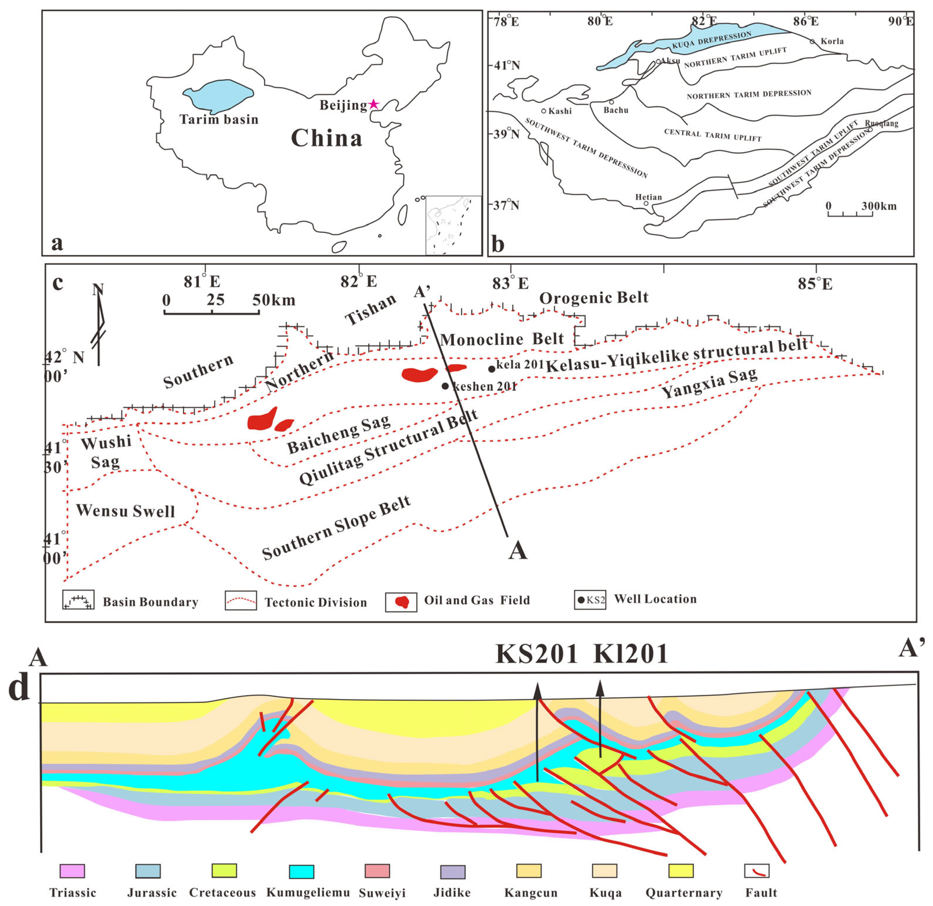
2. Geological Setting

2.1. Structural System

The Tarim Basin in NW China is an important hydrocarbon-producing basin, bordered by the Tianshan Mountains to the north and the Kunlun and Altun Mountains to the south. The basin spans an area of ~560,000 km2 (Figure 1a). The Kuqa Depression is a secondary structural unit located in the northern part of the Tarim Basin (Figure 1b) and is bounded by the South Tianshan Mountains to the north and Northern Tarim Uplift to the south. This basin comprises six structural zones: the Northern Monocline Belt, Kelasu–Yiqikelike Structural Belts, Baicheng–Yangxia Sags, Qiulitag Thrust Belt, Southern Gentle Slope, and Wushi Sag (Figure 1c). The Kelasu–Yiqikelike and Qiulitag Thrust Belts are distinct zones for hydrocarbon accumulation and have resulted in structural systems developed during compressional phases in the time periods shown in Figure 1d. Several giant gas fields, including the Kela-2, DN2, and Dabei gas fields, have been discovered within the Cretaceous and Palaeogene strata [4,18].
Strata in Kuqa Depression were gradually filled from the Triassic to Quaternary periods (Figure 2). During the Triassic period, Ehuobulake (T1oh), Kelamayi (T2k), Huangshanjie (T3h), and Taliqike (T3t) Formations were deposited successively. During the Jurassic period, Ahe (J1a), Yangxia (J1y), Kezilenuer (J2k), and Qiakemale (J2q) Formations were deposited successively. During the Cretaceous period, Yageliemu (K1y), Shushanhe (K1s), Baxigai (K1b), and Bashijiqike (K1bs) Formations were deposited successively. During the Palaeogene period, Kumugeliemu (E1–2km), Suweiyi (E3s), Neogene Jidike (N1j), Kangcun (N1k), and Kuqa (N2k) Formations were deposited successively. This was followed by Quaternary(Q) substratum deposits.

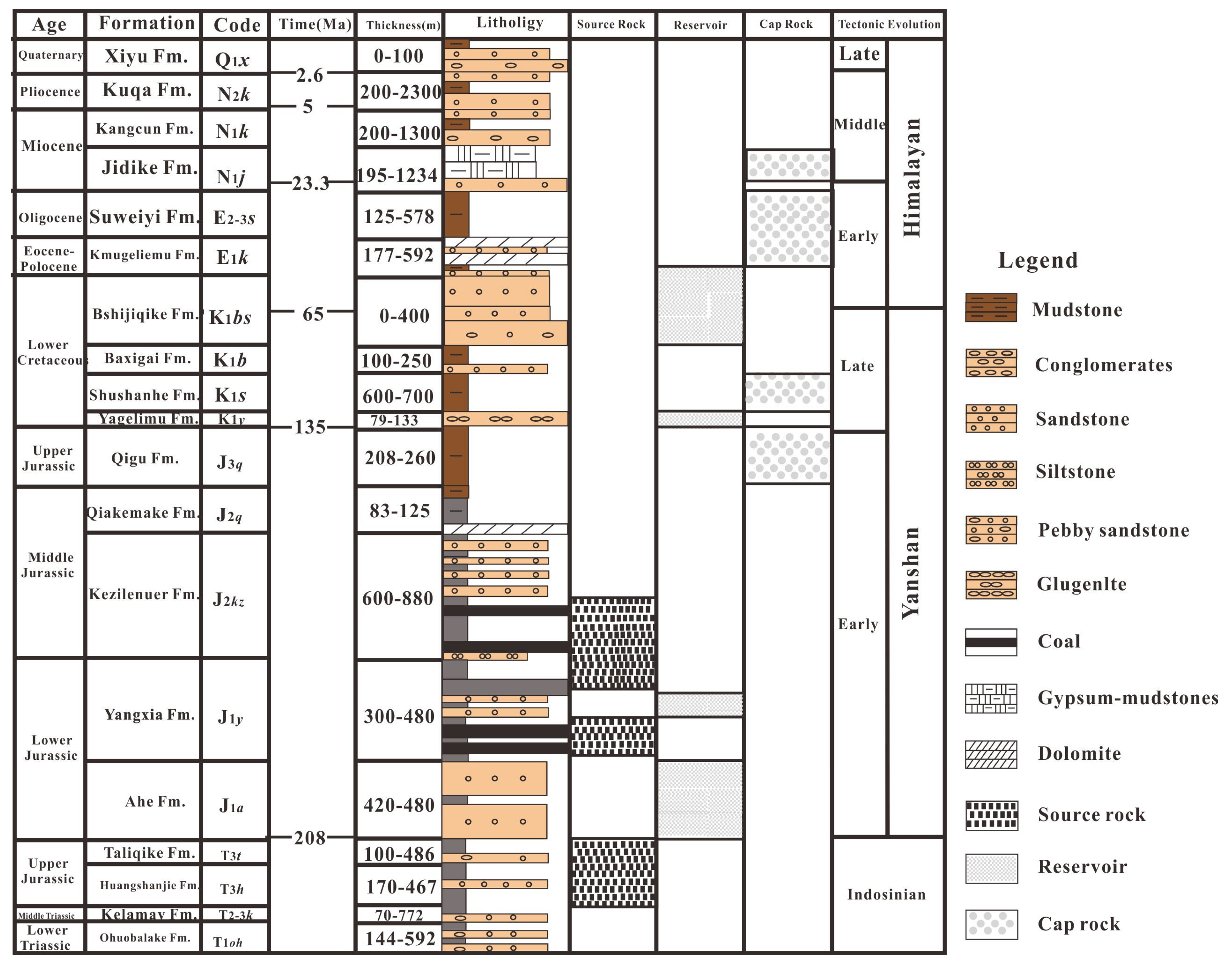
2.2. Petroleum System

The main petroleum source rocks in the Kuqa foreland basin are lacustrine mudstone of Upper Triassic series and lacustrine mudstone of Middle and Lower Jurassic series. The main reservoirs include the following: the sandstone intervals in the Triassic Ehuobulake (T1oh) and Kelamayi (T2k) Formations; the Jurassic Ahe (J1a), Yangxia (J1y), and Kezilenuer (J2k) Formations; and the Cretaceous Baxigai (K1b) and Bashijiqike (K1bs) Formations. The salt and gypsum units in the Eocene Kumugeliemu (E1–2km) and Neogene Jidike (N1j) Formations serve as excellent regional seal rocks. The existence of this fine cap layer is very important for the preservation of oil and gas and the development of abnormal high pressure [18,20].

3. Data and Methods

3.1. Drill Stem Test and Mud Weight Data

Drill stem test (DST) data are the most direct and accurate type of data that can reflect sub-surface pressure. The DST data used in this paper were collected in the report of the Tarim Oilfield Company, PetroChina (Beijing, China). In total, nine DST points were acquired from five wells in the Keshen gas field (KS5, KS501, KS2, KS201, and KS806).
Due to the limited DST data points, which cannot reflect the longitudinal distribution characteristics of pressure, mud density was used to supplement the pressure data. The main advantage of mud density pressure calculation is that it can supplement data points that are not actually measured, and although the corrected data are not completely accurate, direct measurements like the DST data, they are more than enough to reflect the longitudinal distribution of pressure characteristics.
Mud data should be selected before use to ensure their reliability, and the relative error between the mud density and the DST data should be within 10%. Mud weights from four wells (KS801/KS802/KS501/KS201) in the Keshen gas field were finally obtained.

3.2. Well Log and Compaction Curve

Overpressure-related information was extracted from the logging curve to predict and analyze the pressure, owing to the lack of measured data. The logging curves of 10 wells in the Bashijiqike Formation in the Keshen gas field were acquired from the Tarim Oilfield Company, PetroChina.
In pressure research, the accuracy of the compaction curve compilation is vital to ensure a successful evaluation. Compiling compaction curves requires filtering error information and selecting strict data point criteria.
The purpose of compiling the mudstone compaction curve is to extract the pressure-related information from the log, so it is necessary to filter out other useless information. Because of its small specific surface area, mudstone can better preserve pressure information in geological history than sandstone, especially thick mudstone. Compaction and drainage are not smooth, which is more likely to cause unbalanced compaction and cause overpressure.
The expanding effect causes an abnormal acoustic time difference, so the information of the expanding part was not used. In order to ensure that it was mudstone, gamma logging was used to determine that the mudstone content was greater than 75%. In order to ensure the thickness of the mudstone, mudstone with a thickness greater than 10 m was selected. In order to ensure the continuity of the final result, an effective data point was required to be taken within 20 m.

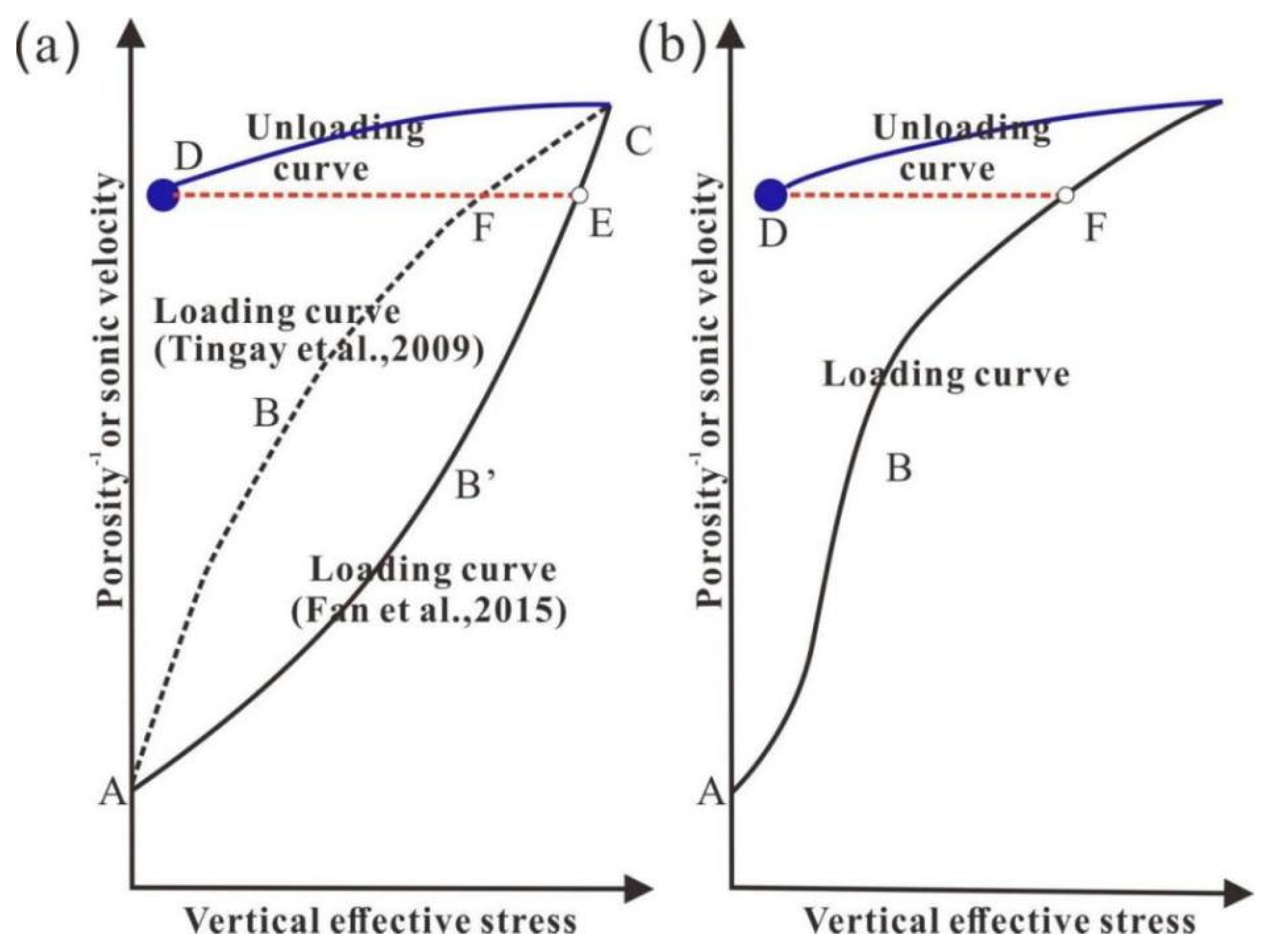
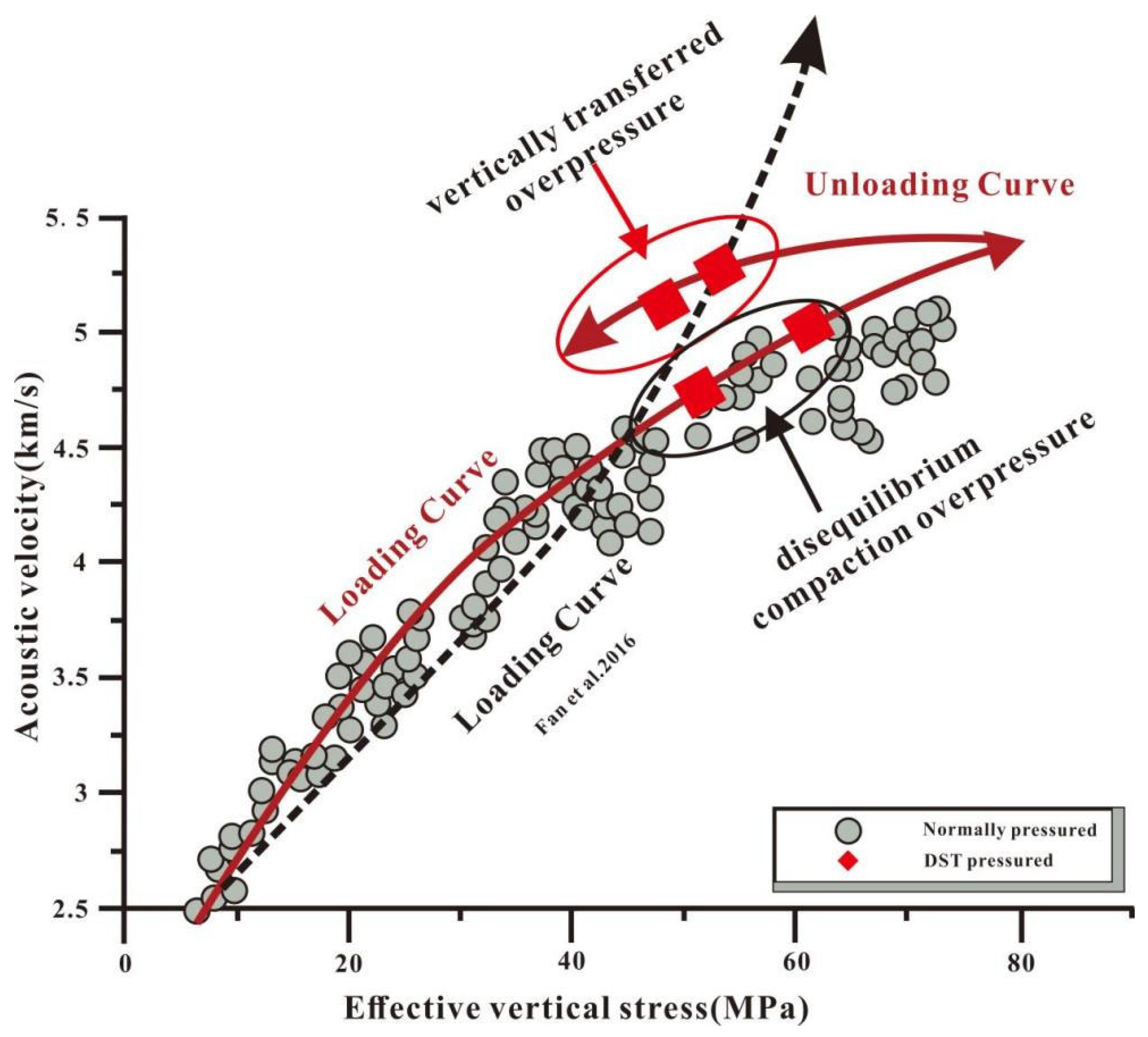
3.3. Acoustic Transit–Vertical Effective Stress Crossplots

Two typical wells (KS201 and KS8003) in the Keshen area were selected. The vertical effective stress equals the difference between the overburden (static rock pressure) and the pore pressure. The static rock pressure was calculated using the formula in Appendix A. The pore pressure was calculated from the compacting curve using the equivalent depth method. The sound velocity was calculated by the reciprocal of the acoustic time difference, thus yielding the loading curve of the sound velocity–effective stress chart.

3.4. Earth Stress Field Simulation

In this study, Rhino software (version 10.0) and Ansys Workbench 17.0 were used to establish the geological model and simulate the ground stress, respectively.
The simulation was divided into four steps. ① Steps to determine the model type: determine the analysis type and model type. ② Pre-processing steps: build imported geometric models, define material properties, and divide grids. ③ Solution step: apply the load and constraint and solve. ④ Post-processing: view the conclusion, draw a conclusion, and test the correctness of the result (Figure 3).
The analysis type of this study is static analysis; the unit type is the entity unit.
The imported geometric model was the geological model of the Bashiqik Formation. Material properties were determined by selecting the physical properties of the sand and mud data. Previous research obtained the physical parameters of rocks in the northern Tarim Basin by studying the common uniaxial and triaxial rock mechanics [14]. The grid division used the hexahedral type. The solution step meant that the direction and magnitude of the applied load were constrained by the experimental results. In this study, previous experimental data on paleo-tectonic deformation and the magnetic fabric of rocks were used to determine the direction of the stress field in the Kuqa Depression. This paper quotes the research results of previous research [14]. Acoustic emission testing was used to determine the size of the paleo-tectonic stress field. In the postprocessing, finally, a tectonic compression stress of 100 MPa was applied to the northern part of the model. A displacement constraint was imposed on the fixed boundary in the south, and an additional 70 MPa stress was applied to the fixed boundary displacement constraints in the east and west. The load and gravity were applied vertically to account for the weight of the overburden. The relative error between the final result and the experimental result was less than 10%.

3.5. Basin Simulation

The 1D/2D module of PetroMod2012 software (Schlumberger) was used to simulate pressure evolution. The simulation process calibrated the burial, lithology (porosity), and pressure processes. The data required in the simulation process can be divided into three categories: basic data (non-adjustable), adjustable parameters, and calibration data. The simulation first built the basic data, adjusted the parameters, and continuously approximated the calibration data.
The basic data used to simulate the burial history were the top and bottom depth, erosion thickness, formation deposition time, and erosion time of each layer. The above data were acquired from the Tarim Oilfield Company, PetroChina. The parameters to be adjusted were the geological framework generated during the simulation. The calibration data represented the actual geological situation.
The basic data for the simulation of the lithology (porosity) were the sedimentary facies distribution and well lithology information. The porosities of the sand and mudstone were calculated using the Wiley formula (see Appendix A) after the compaction curve was compiled from the logging curve. The effective stress of the sand and mudstone was obtained by subtracting the pore pressure (calculated by the equivalent depth method after the compaction curve was compiled by the log) from the overburden (S = ρgh). The parameter to be adjusted was the porosity (Figure 4c)–effective stress (Figure 4b) relationship. The calibration data were the measured porosities. The sedimentary facies, well lithology information, and the measured porosity were all obtained from the Tarim Oilfield Company, PetroChina.
The basic parameter of the overpressure simulation of the disequilibrium compaction type was the porosity (which was calibrated during the simulation). The parameters to be adjusted were the permeability, porosity relationship, and compaction coefficient. The calibration data were the pressures calculated using the equivalent depth method after the compaction curve had been compiled using the logging curve.
This time, the results of structural extrusion after quantitative evaluation were added to the results of the unbalanced compaction type of overpressure in the form of boundary conditions.
The basic parameters of the fracture transfer overpressure simulation were the shape and distribution characteristics of the fracture and the opening time of the fracture. The parameter to be adjusted was the permeability of the fault, and the calibration data were the amounts of fault transfer overpressure after quantitative evaluation. The Tarim Oilfield Company, PetroChina, provided the fault morphology and distribution characteristics. Between 2.48 and 1.75 Ma, all faults are considered open and active, allowing fluid flow [4,18].
Limitations of modeling: the limitations of the model are that the tectonic extrusion and fracture transfer overpressure are only considered to be instantaneous events, and the model could be improved if there is a better idea in the future.
Circumscribed effects: The limitation of the assumption that tectonic compressions are instantaneous affects the accuracy of the evolutionary results of tectonic compressions. The assumption that the fault transmission type overpressure is also an instantaneous opening is not consistent with actual fault curtain openings. But, there is no better way to solve the model’s aim.

4. Results

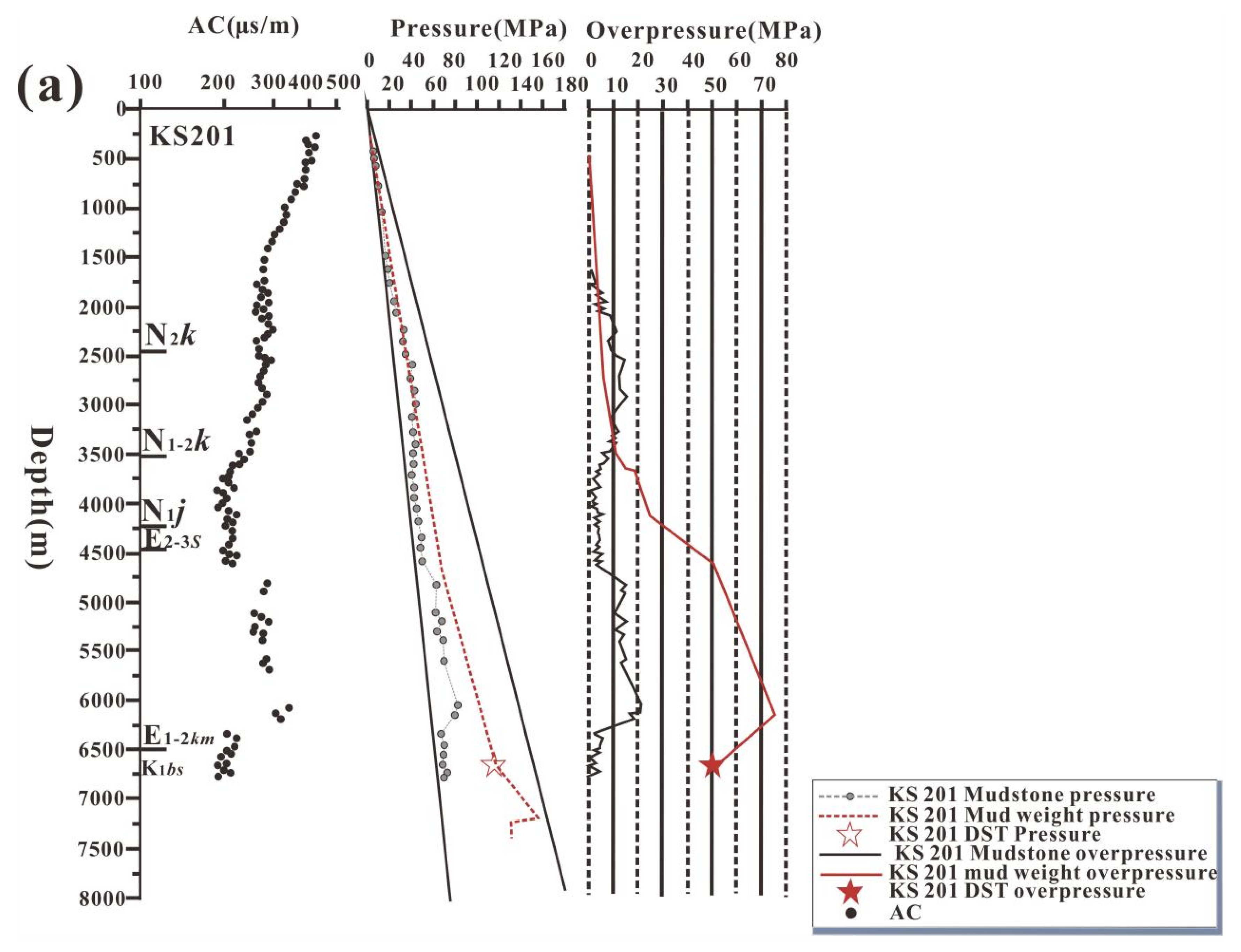
4.1. Overpressure in Sandstones

The residual pressure in the Keshen area showed a trend of gradually increasing from top to bottom and then decreasing. However, the residual pressure distribution in the longitudinal direction in different well areas was slightly different. In the Keshen 8 well area, the distribution of residual pressure in the longitudinal direction showed an obvious four-stage pattern. The residual pressures in the 0–2000 m, 2000–6500 m, 6500–7000 m, and 7000–8000 m ranges were 0–5 MPa, 5–50 MPa, 50–90 MPa, and 60–90 MPa, respectively. In the Keshen 5 well area, the residual pressure distribution in the longitudinal direction showed an obvious three-stage pattern. The residual pressures in the 0–2000 m, 2000–5000 m, and 5000–7000 m ranges were 0–20 MPa, 20–60 MPa, and 40–60 MPa, respectively. In the Keshen 2 well area, the longitudinal distribution of the residual pressure showed an obvious four-stage pattern. The residual pressures in the 0–3500 m, 3500–4500 m, 4500–6500 m, and 6500–7000 m were 0–10 MPa, 10–60 MPa, 60–90 MPa, and 50–90 MPa, respectively (Figure 5).

4.2. Characteristics of Mudstone Compaction Curve

Two typical wells (KS201 and KS802) in the Keshen area were selected to study the characteristics of the mudstone compaction curves (Figure 6). The gamma, resistivity, and sonic time difference curves showed prominent four-stage characteristics in the longitudinal direction. In the Kuche Formation, the gamma curve showed a basic stable value, and the resistivity curve showed a linear increase. The time difference curve of the sound wave decreased linearly. The gamma curve in the Kangcun Formation, Gidike Formation, and Suweiyi Formation showed a basic stable value. The resistivity curve showed a trend of first increasing and then decreasing, and the sonic time difference curve showed a trend of first decreasing and then increasing. In the Kumglimu Formation, the gamma curve showed a basic stable value; the resistivity curve reached the minimum, and the sonic lag curve reached the maximum. The gamma curve was basically stable in the Bashijiqike group. The resistivity increased, and the time difference in the sound wave decreased.

4.3. Characteristics of Acoustic Transit–Vertical Effective Stress Crossplot

Two typical wells (KS201 and KS802) in the Keshen area were selected to study the characteristics of the intersection diagram (Figure 7). The characteristics of the intersection diagram of sound velocity and effective stress in the Keshen region were as follows. The effective stress ranged from 0 to 85 MPa, and the sound velocity ranged from 2.5 to 5.5 km/s. The loading curve presented a log-like feature. The data points calculated for the measured pressure included those on the loading curve and those on the unloading curve, and the degree of deviation from the loading curve varied among the wells. The degree of deviation from the loading curve was weak in well KS201 and strong in well KS8003.

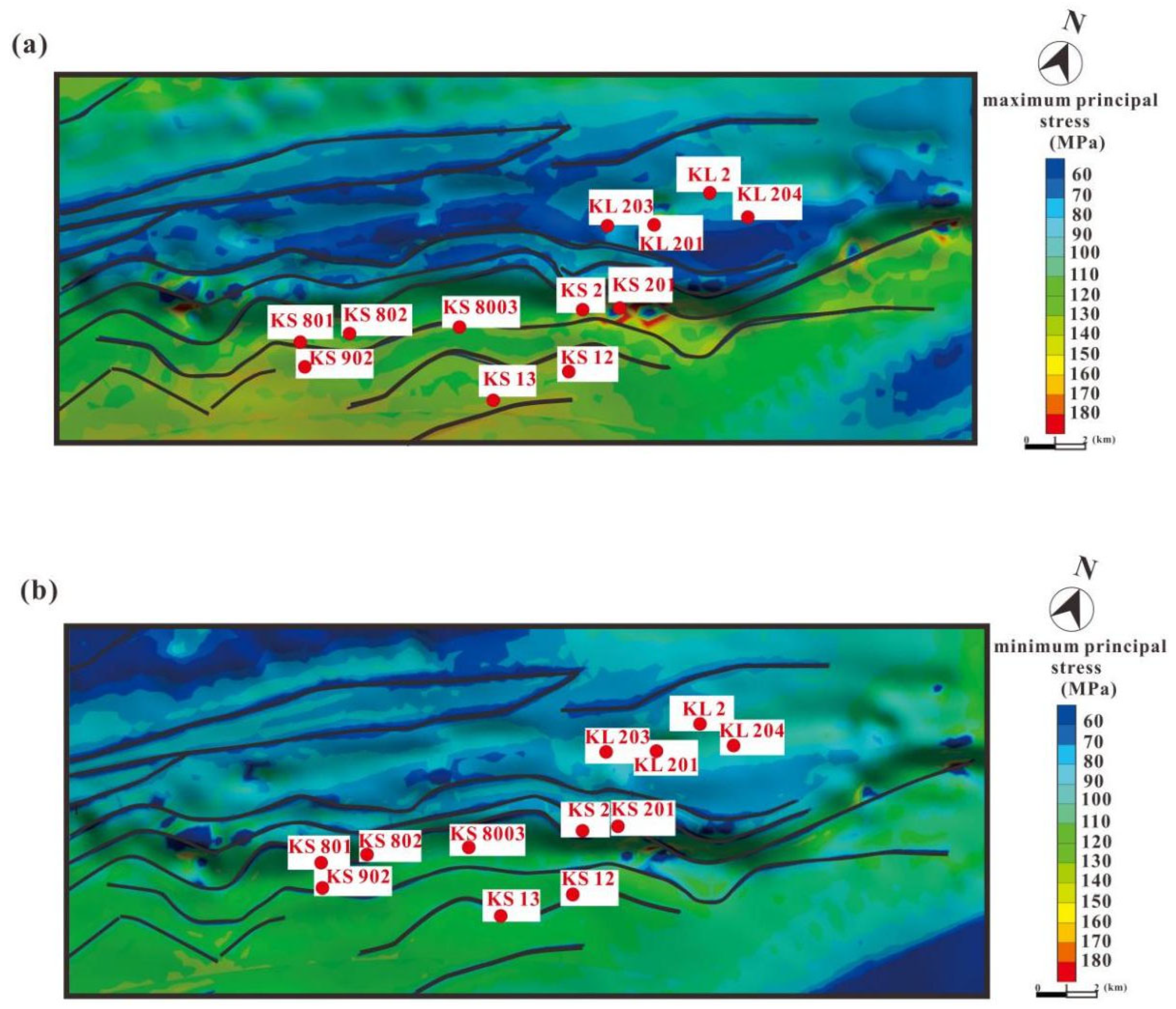
4.4. Earth Stress Distribution

Figure 8a shows the distribution characteristics of the maximum principal stress in the surrounding regions of Keshen. Except for the fault region, the maximum principal stress ranged from 150 to 180 MPa in the Keshen region, with the lowest value observed near the fault at ~60 MPa. The highest value area was located near the well KS2, measuring ~180 MPa. The well KS8 experienced a maximum principal stress value of 150–160 MPa, while the well KS9 exhibited a similar range of 150–160 MPa for its maximum principal stress. In the well Keshen 2, the residual pressure fell between 150 and 180 MPa. Figure 8b shows the distribution characteristics of the minimum principal stress in the relevant areas surrounding the Keshen region. Excluding the fault area, the minimum principal stress within this region ranged from 80 to 120 MPa, reaching its lowest point near both faults and northwest regions at ~60 MPa while peaking in the southwest areas at 110–120 MPa. The minimum principal stresses for the wells KS8 and KS9 fell within 110–130 MPa, whereas the minimum principal stress for the Keshen well 2 was between 70 and 100 MPa.

4.5. Basin Modelling Results

The simulation results of a single well, Keshen 201, serve as an illustrative example. The porosity simulation revealed a range of 2–40%, with the Bashijiqike Formation exhibiting a porosity of 7%, which is in good agreement with the measured data (Figure 9a). The pressure simulation results indicated that the residual pressure resulting from disequilibrium compaction was approximately 15 MPa, while the excess pressure caused by structural extrusion amounted to approximately 30 MPa. In addition, the excess pressure attributed to fracture transfer was ~15 MPa (Figure 9b). The simulation results of the burial history suggest that before 23.3 Ma, minimal alterations occurred in the strata. In contrast, between 10 and 23.3 Ma, the depth of the strata increased significantly by up to 4000 m. Subsequently, from 2.48 Ma to the 21st century, there was a rapid increase in the burial depth, reaching up to 8000 m for the stratum (Figure 9c). The simulation results indicate that before 23.3 Ma, the deposition rate remained extremely low, approaching zero. Between 10 and 23.3 Ma, the deposition rate was below 0.2 km/Ma. From 2.48 to 10 Ma, there was a rapid increase in the deposition rate, reaching up to 2 km/Ma. A significant decline in the deposition rate was observed from 2.48 Ma until the present (Figure 9d).

5. Discussion

5.1. Quantitative Evaluation of Overpressure

5.1.1. Mudstone Disequilibrium Compaction Overpressure

The integrated compaction curve method is one of the most reliable methods for identifying the causes of pressure, especially for the identification of disequilibrium overpressure. The abnormal pressure caused by disequilibrium compaction is shown in the compaction curve in that the acoustic wave propagation time of abnormally high-pressure mudstone is longer and the resistivity is lower even if there is no porosity anomaly [21,22].
Two representative wells (KS201 and KS802) in the Keshen area were used to study the unbalanced compaction. Figure 6 presents the acoustic time difference, gamma data, and resistivity. The resistivity and acoustic time difference in the Kuche Formation showed a normal compaction trend. The acoustic time difference and resistivity curves from the bottom of the Kucha Formation showed a significant deviation from the normal compaction trend, and both responded to disequilibrium compaction. The degree of deviation from the bottom of the Kucha Formation was different and could be divided into a weak unbalanced compaction section, a strong unbalanced compaction section, and a medium unbalanced compaction section from top to bottom. The weak unbalanced compaction sections were the Kangcun, Jidike, and Suweiyi Formations. The strong disequilibrium compaction section was the Kumgremu Formation and the medium disequilibrium compaction section was the Bashijiqike Formation.
The quantitative evaluation of the overpressure of a disequilibrium compaction type is usually conducted using the equivalent depth method (Figure 10) on a compiled mudstone compaction curve (Figure 6). The equivalent depth method was used to calculate the acoustic time difference logs of three typical wells in the Keshen area to study the pressure induced by disequilibrium compaction (Figure 7). The overpressures resulting from disequilibrium compaction varied significantly across the vertical profile in the Keshen area. The residual pressure originated from the base of the Kuqa Formation, with the residual pressure range in the Kangcun, Jidike, and Suweiyi Formations being 0–10 MPa. The residual pressure ranges of the Kumgelemu and Bashijiqike Formations were 15–40 and 5–10 MPa, respectively. The overpressure induced by disequilibrium compaction in the Bashijiqike Formation was compared with the measured DST data. The results reveal a significant difference. Therefore, the overpressure in the Bashijiqike Formation in the Keshen area was caused by multiple factors.

5.1.2. Transfer Overpressure

The intersection diagram of sound velocity and vertical effective stress can be used to determine the cause of different overpressures, and the location of the unloading curve indicates that the overpressure is due to fluid transfer (vertical or lateral fluid flow) or fluid expansion [5,9,23]. In permeable sandstone, points located on the unloading curve are usually caused by fracture transmission [12].
The fracture transfer overpressure deviates from the loading curve in the intersection diagram of sound velocity and vertical effective stress (Figure 6). It remains on the unloading curve, with a slight decrease in the sound velocity and a significant decrease in the vertical effective stress. The quantitative calculation of fracture transfer overpressure is usually carried out by applying a suitable mathematical quantitative evaluation model to a sound velocity–effective stress chart. Previously, a quantitative evaluation method for fracture transmission was established [11]. However, the loading curve in its exponential form was inapplicable to the deep area under the tectonic compression background of Keshen (Figure 6). Therefore, this study improved this loading curve by establishing a more suitable quantitative evaluation model of fault-transmitted overpressure in the deep foreland basin (see Appendix A). The calculation revealed a transfer overpressure of 15–20 MPa in the Keshen area.

5.1.3. Tectonic Compression Overpressure

When the minimum principal stress is relatively high, or even close to the vertical effective stress, the overpressure caused by horizontal structural extrusion is considered an important pressure formation mechanism [13]. According to the above calculation, the vertical effective stress in the Keshen area was approximately 130–150 MPa. The maximum horizontal principal stress (150–180 MPa; Figure 7a) > the vertical overlying rock pressure (130–150 MPa) > the minimum horizontal principal stress (80–120 MPa; Figure 7b) of the Bashijiqike Formation in the Keshen Area. Several studies have also shown that tectonic compressional overpressure is the main formation mechanism of overpressure in the Kuqa Depression [14,18]. Overpressure caused by tectonic compression can be considered unbalanced lateral compaction, which reduces porosity and permeability and leads to poor drainage, resulting in the tectonic compression type of overpressure. Therefore, the role of tectonic stress in overpressure generation in the Keshen area cannot be ignored.
The quantitative evaluation of structural extrusion overpressure is usually based on the obtained data of maximum and minimum principal stresses (Figure 7), which are brought into a corresponding mathematical model. Tectonic compression and pressurization are important mechanisms of overpressure formation, and the burial depth in the Keshen area is significant (4000–7100 m). Byerlee’s friction slip curve and the plastic deformation curve were established according to Byerlee’s friction law and the Goetze criterion. The Keshen area is characterized by brittle–brittle plasticity. Therefore, the quantitative evaluation model of the pore fluid compression and pressurization of brittle—brittle plastic rocks was selected (see Appendix A).
According to the equation, the residual pressure generated by the structural compression type of overpressure in the Keshen area was 25–30 MPa.

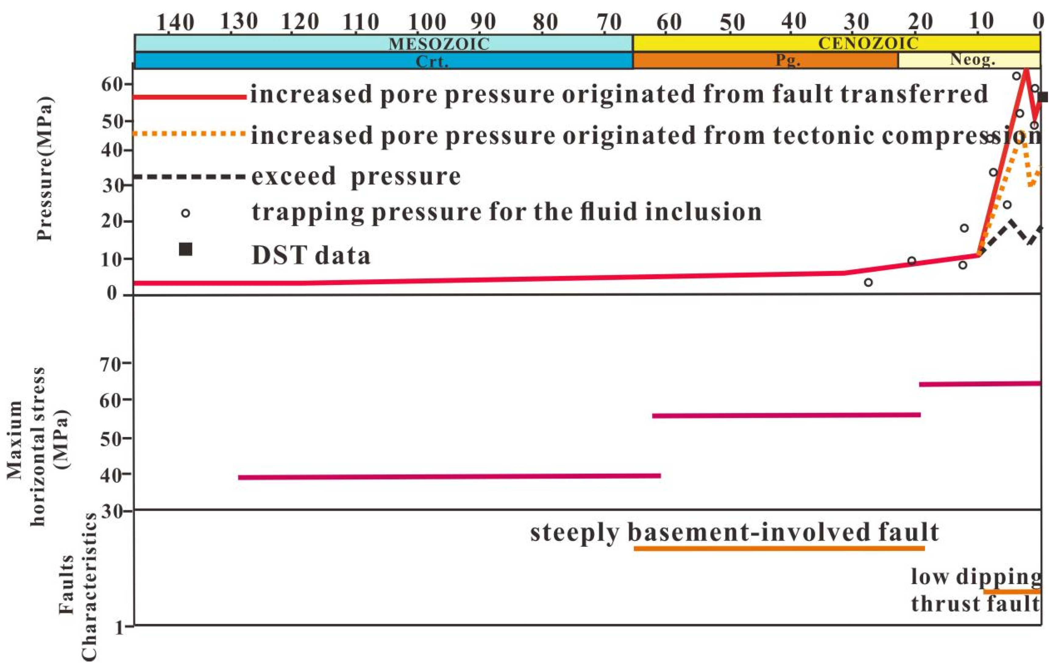
5.2. Overpressure Evolution

The restoration and reconstruction of paleo-pressure poses significant challenges in petroliferous basins. Herein, the evolution characteristics of deep overpressure in the foreland basin (Figure 11) and the coupling evolution characteristics of multi-genetic pressure were analyzed (Figure 12) by combining the formation mechanism of the overpressure with the characteristics of the tectonic compression, fault development, burial history, and deposition rate, considering the DST-measured pressures as constraints.

5.2.1. Individual Well Pressure Evolution

The evolution of the disequilibrium compaction overpressure is consistent with the sedimentation rate. Before the deposition of the Neogene Formation (23.3 Ma), the sedimentation rate was very low and the unevenly compacted overpressure was almost zero. The deposition rate of the formation was <0.2 km/Ma before the rapid burial of the formation (10–23.3 Ma). During this period, the compaction and drainage were balanced, and the overpressure due to the disequilibrium compaction was <10 MPa. The deposition rate increased rapidly with the rapid burial of the formation, leading to a corresponding increase in the disequilibrium compaction overpressure. This pressure reached a maximum of 18 MPa at the maximum burial depth of the formation (2.48 Ma). At 2.48 Ma, the tectonic compression was enhanced and the residual pressure reached ~50 MPa under the pressurization of the tectonic compression. At 1.75–2.48 Ma, the fracture activity was enhanced, leading to the generation of the fracture transfer overpressure. Under its influence, the residual pressure exceeded 60 MPa. Subsequently, there was a slight pressure release as the formation underwent uplift.

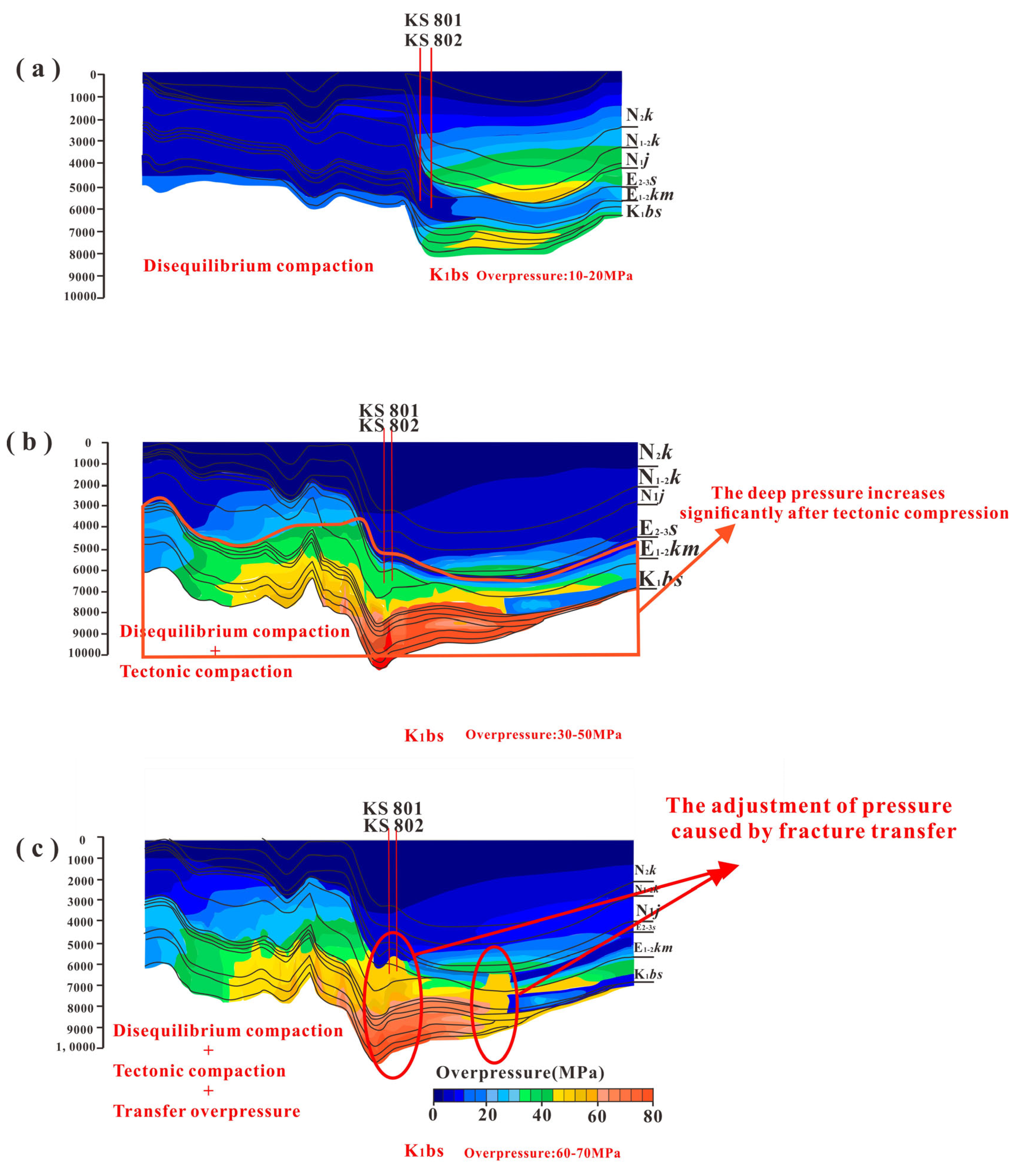
5.2.2. Multi-Genetic Profile Pressure Evolution Profile

Considering the profile of well 8 in the Keshen area as a typical example, this study analyzed the characteristics of multi-genetic pressure coupling evolution in the Keshen area (Figure 12).
The residual pressure of the disequilibrium compaction type was low in the shallow part and high in the deep part. The thick ductile salt layer, source rock, and Baicheng Sag showed high residual pressures (Figure 12a).
After the tectonic compression, the residual pressure increased from top to bottom in the profile, and the residual pressure increased significantly in the deep part (Figure 12b). This observation was attributed to the maximum principal stress of the Kuqa Depression being inconsistent at different depths, showing a good linear relationship with the depth. The maximum principal stress increased as the depth increased until the structural extrusion type of overpressure was observed.
After fracture transmission occurs, the two completely separate pressure systems are connected through an open fault, and the pressure is re-adjusted through the fault, eventually reaching a new equilibrium, and the two pressure systems are spatially regrouped and ordered [23,24]. This phenomenon is called “pumping” action. Therefore, after the fracture transfer action, the residual pressure in the ductile salt layer near the fracture increased, decreasing significantly in the deep layer near the fracture (Figure 12c).

6. Conclusions

In the Keshen area of the Kuqa Depression, the following conclusions were obtained through the combination of measured well data (DST and mud data), well logging data, experimental data (acoustic emission experiment), a mathematical quantitative evaluation model (fault transmission and tectonic extrusion), and numerical simulations (Petromode and Ansysworkbench).
The overpressure of the Bashijiqike Formation in the Keshen area of the Kuqa Depression was quantitatively evaluated as follows. The overpressure caused by disequilibrium compaction was 5–10 MPa, the overpressure caused by tectonic extrusion was 25–30 MPa, and the overpressure caused by fault transmission was 10–15 MPa.
The characteristics of pressure evolution in a single well in the Keshen area were as follows. Before the deposition of the Neogene strata (23.3 Ma), the disequilibrium compaction overpressure was basically zero. Subsequently, with the gradual increase in deposition, the residual pressure caused by disequilibrium compaction reached 18 MPa at the maximum burial depth of the formation. Simultaneously, the tectonic compression was enhanced, and the residual pressure reached ~50 MPa under the pressurization of tectonic compression. Subsequently, the fracture activity was enhanced, and the formation underwent an uplift.
The profile coupling characteristics of multi-genetic pressure in the Keshen area were as follows. The residual pressures of the tectonic compression overpressure were low and high in the shallow and deep parts, respectively. The thick ductile salt layer, source rock, and Baicheng Sag showed high residual pressure values. After tectonic compression, the residual pressure increased from top to bottom in the profile, and the residual pressure increased significantly in the deep part. After fracture transmission, owing to the “pumping” effect, the residual pressure in the ductile salt layer near the fracture increased significantly, whereas it decreased significantly in the deep layer near the fracture.

Author Contributions

Writing—original draft, C.W.; Writing—review & editing, C.W.; Project administration, Z.W.; Funding acquisition, Z.W. All authors have read and agreed to the published version of the manuscript.

Funding

This study was co-funded by the Important National Science Foundation (2017ZX05008004-004).

Institutional Review Board Statement

Not applicable.

Informed Consent Statement

Not applicable.

Data Availability Statement

Data are contained within the article.

Acknowledgments

We thank PetroChina Tarim Oilfield Company for providing well data.

Conflicts of Interest

The authors declare no conflict of interest.

Appendix A

  • Technical terms
  • Mudstone disequilibrium compaction overpressure
Disequilibrium compaction is essentially due to an imbalance between compaction and drainage. Previous studies have shown that the main factors affecting disequilibrium compaction are the deposition rate and mud content. The greater the deposition rate, the less favorable the directional arrangement of mudstone particles, and the more likely it is to lead to an imbalance between compaction and drainage, resulting in disequilibrium overpressure. In the sand–mudstone interlayer, the high sandstone content makes the overpressure in mudstone easy to transfer upward and downward, and the drainage is smooth, which is not conducive to the formation of the unbalanced compaction type of overpressure. However, in principle, the factors that can cause an imbalance between compaction and drainage can produce the disequilibrium compaction type of overpressure.
  • Transfer overpressure
When two pressure systems are connected by an open fault, the fluid pressure quickly adjusts to reach hydrostatic equilibrium, and a new pressure system is formed, which is caused by the spatial realignment of the fault into a fault-transmitted overpressure.
  • Tectonic compression overpressure
The tectonic extrusion type of overpressure is lateral compaction caused by tectonic extrusion.
  • Multi-genetic overpressure
Multi-cause pressure means that the cause of pressure is not a single cause but that, in the process of geological evolution, there have appeared different causes of pressure or there have been two kinds of pressure simultaneously.
  • Pressure evolution
This refers to the change in pressure over time in geological history.
  • Static rock pressure
S = ρgh
where S represents the static rock pressure, ρ denotes the average density of the overburden material, g represents the average gravitational acceleration, and h denotes a certain depth.
  • Wiley formula
φ = ( t t m a ) C p ( t f t m a )
  • Brittle deformation
Brittle deformation refers to the deformation of an object without significant strain (less than 5%).
  • Plastic deformation
    Plastic deformation is a deformation that cannot be restored by itself. Engineering materials and components will be permanently deformed after the load exceeds the elastic deformation range, that is, after the load is removed, there will be unrecoverable deformation, or residual deformation, which is plastic deformation.
  • Quantitative evaluation model of fault-transfer overpressure in the deep layers of a foreland basin:
The process of developing the new model is as follows:
Under normal compaction, porosity is exponential concerning depth:
φ = φ 0 e c z
where φ and φ 0 represent the Z depth and surface mudstone porosity (Z = 0), respectively; e is the base of the natural logarithm; and C is a constant.
The relationship between porosity and acoustic time difference can be expressed by the Wiley equation:
φ = ( t t m a ) C p ( t f t m a )
where φ is the acoustic time difference to calculate porosity.
t m a  and  t f are the acoustic time difference in the rock skeleton and formation fluid. C p is the acoustic compaction correction coefficient. t is the acoustic time difference logging value of the target layer.
According to Equation (A1), we can obtain the following:
z = [ g ( ρ b ρ w ) ] 1 σ
where ρ b is the density of the rock, ρ w is the density of water, g is the acceleration due to gravity, and σ is the effective vertical stress.
Furthermore,
v = 1 t
where t is the acoustic time difference logging value of the target layer and v is the sound velocity value of the target layer.
By substituting Equations (A1)–(A3) into Equation (A4), the relationship between sound velocity and effective stress can be obtained as follows:
v = 1 C p ( t m a ) φ 0 e c g ( ρ b ρ w ) σ + t m a
where v is the sound velocity value of the target layer, t m a  and  t f are the acoustic time difference in the rock skeleton and formation fluid, and C p is the acoustic compaction correction coefficient. In addition, ρ b is the density of the rock, ρ w is the density of water, g is the acceleration due to gravity, and σ is the effective vertical stress. Furthermore, φ 0 represents the surface mudstone porosity (Z = 0), e is the base of the natural logarithm, and C is a constant.
To determine the shape of the loading curve, Equation (A5) is considered a function. It is found to be monotonically increasing; upon evaluating its second derivative, it exhibits both concave and convex regions. Consequently, the improved loading curve exhibits an initial phase of exponential growth followed by logarithmic growth (Figure A1b). The improved loading curve is more consistent with the compaction process. During deposition, as the burial depth increases, the vertical effective stress rises, resulting in a decrease in porosity and an increase in sound velocity. However, as the overburden increases, the rates of change in vertical effective stress, porosity, and sound velocity vary significantly across different sedimentary periods. At the beginning of deposition, pore fluid compaction and drainage are balanced, with the overburden fluid pressure borne by the fluid and the overburden skeleton pressure borne by the skeleton. Consequently, porosity decreases rapidly with increasing vertical effective stress, and sound velocity increases rapidly with increasing vertical effective stress, exhibiting a quasi-exponential shape on the loading curve (section AB of Figure A1b). As compaction begins and pore fluid compaction and drainage become imbalanced, the pressure that would otherwise be borne by the skeleton is now borne by the fluid. Consequently, porosity slowly decreases as vertical effective stress increases, and the speed of sound increases slowly with increasing effective vertical stress. On the loading curve, it presents a log-like shape (section AC of Figure A1b). The net effect of compaction is a gradual reduction in porosity towards zero, although it never fully reaches zero. Similarly, the speed of sound approaches the skeleton speed but never quite reaches it, as depicted by the asymptotic line in Figure 8b.
Figure A1. Comparison between the new quantitative evaluation model of fracture transfer overpressure and the original model. (a) Original sonic velocity−effective stress schematic [5,11]. (b) Newly established sonic velocity−effective stress schematic suitable for deep foreland basins.
Sustainability 16 10884 g0a1
It can be seen from the previous analysis that fracture transmission will cause a reduction in the effective stress of the pressurized section, and the reduction (section DF in Figure A1b) is exactly equal to the transmitted overpressure value. Based on this, the calculation formula of fracture transfer overpressure can be approximated as follows:
P t δ F δ D = l n 1 v F t m a φ 0 C p ( t t m a ) · g ( ρ b ρ w ) c δ D = l n 1 v D t m a φ 0 C p ( t t m a ) · g ( ρ b ρ w ) c
where P t is the amount of overpressure caused by the fracture transmission, δ F is the effective vertical stress at point F, δ D is the effective vertical stress at point D, vF is the sound velocity value at point F, vD is the sound velocity value at point D, t m a ,   t f are the acoustic time difference in the rock skeleton and formation fluid, and C p is the acoustic compaction correction coefficient. In addition, ρ b is the density of the rock, ρ w is the density of water, g is the acceleration due to gravity, and σ is the effective vertical stress. Furthermore, φ 0 represents the surface mudstone porosity (Z = 0), e is the base of the natural logarithm, and C is a constant.
  • Advantages of model
The fracture transfer overpressure model is compared with the existing model:
The original fracture transfer overpressure model is exponential, and it is found that it cannot fully fit the acoustic velocity effective stress template in the deep foreland basin during fitting. Therefore, if the previous method was to be used for calculation, the error would be large. The new model is logarithmic and has a good fit with the acoustic velocity and effective stress in the deep background of the foreland basin, with a higher calculation accuracy.
Figure A2. Sonic velocity–effective stress (SV-ES) schematic obtained by calculation in the well KS201, fitting the original and newly established loading curves. The original loading curve is in the form of quasi-exponential; it cannot be fitted to the actual situation of well KS201. The newly established loading curve has a log-like morphology; it is more in line with the actual situation of well KS201 [11].
Sustainability 16 10884 g0a2
  • Limitations of the model
It is only suitable for deep foreland basins.
  • Application of model
Keshen 201 is taken as an example to illustrate the results of this model. First, the template diagram of the effective stress of the sound velocity is prepared, as shown in Figure 7. According to the A6 formula, two DST data points on the unloading curve can be put into the above formula to obtain the amount of fracture transfer type overpressure.
  • Quantitative evaluationmodel of tectonic compressional overpressure in deep foreland basin
The deformation of brittle and brittle–plastic rocks can be divided into two main stages: elastic deformation and plastic deformation. By analyzing the physical process of structural compression deformation, the elastic deformation and plastic deformation of brittle and brittle–plastic rocks can be further categorized into volume deformation and shape deformation.
Elastic   deformation :   ε e = ε e v + ε e θ
Plastic   deformation :   ε p = ε p v + ε p θ
where εe is the elastic deformation; εev and εeθ are the volume deformation and shape deformation in the elastic deformation process, respectively; εp is the plastic deformation; and εpv and εpθ are the volume deformation and shape deformation in the plastic deformation process, respectively.
Based on the above analysis, we assume a certain functional relationship between the volume deformation and shape deformation in the deformation of brittle and brittle–plastic rocks, as follows:
ε v ε θ = F ( σ )
where εe and εθ are the volume deformation and shape deformation in rock deformation, respectively, and indicate the stress experienced by the rock.
Thus, the relationship between plastic deformation and elastic deformation can be further expressed as follows:
ε p ε e = ε p v + ε p θ ε e v + ε e θ = [ 1 + ( F ( σ ) ) ] ε p v [ 1 + ( F ( σ ) ) ] ε e v = k
where k is the ratio of volume deformation in plastic deformation to volume deformation in elastic deformation.
Thus, the deformation in the rock can be expressed as follows:
ε = ε e + ε p = ( 1 + k ) · ε e
According to the stress–strain relationship at the elastic stage, the porous elastic equation can be expressed as follows:
ε e i j = 1 2 u ( σ i j 1 3 σ m δ i j ) + 1 3 B σ m δ i j
By substituting Equation (A6) into Equation (A5), we obtained the stress–strain equation of the rock, as follows:
ε ij = ( 1 + k ) ε e i j = ( 1 + k ) [ 1 2 u ( σ i j 1 3 σ m δ i j ) + 1 3 B σ m δ i j ]
where εij is the strain tensor; σij is the effective stress tensor; σm is the average effective stress; u and B are the shear and volume moduli, respectively; and δij is the Kronecker symbol. Tectonic compression produces additional deformation, e, along the horizontal direction e, where σ 33 = σ v is the vertical effective stress, σ 22 = σ H is the horizontal maximum effective stress, and σ 11 = σ h is the horizontal minimum effective stress, given that ε 11 = 0 , ε 22 = e , ε i j = 0   ( i j ) , σ 33 = σ v , and σ i j = 0   ( i j ) .
By solving Equation (A6), the stress relationship of brittle and brittle–plastic rocks at the point of failure can be obtained as follows:
σ v = σ h v σ H
where v is Poisson’s ratio of the rock.
The fluid pressure at the fracture point (maximum fold stage) can be calculated using the characteristic equation, as follows:
P r = S v σ v
where Sv is the overburden of the rock at the point of rupture.
Thus, the pressurization amount of tectonic extrusion fluid is as follows:
Δ P = P r P m
where Pm is the fluid pressure during the maximum burial depth of the rock.
  • Advantages of model
Comparison between the structural extrusion overpressure model and the existing model:
A lot of work has been conducted on the relationship between rock structural stress and abnormal pore fluid pressure, and the corresponding quantitative evaluation model of tectonic compression and pressurization has been proposed. It includes the following: the quantitative evaluation of the upper limit of the contribution of structural extrusion to overpressure based on a plane stress field, the quantitative evaluation of the contribution of structural extrusion based on a plane stress field to overpressure in a semi-closed system, the quantitative evaluation of the contribution of a numerical simulation based on a three-dimensional stress state to overpressure, etc. However, these models have many solving parameters, are easily affected by human factors, or lack the consideration of rock deformation process, deformation mechanisms, and pressure evolution, which limits the applicability and operability of the models to a certain extent.
  • Limitations of the model
It is only suitable for deep foreland basins.

References

  1. Hao, F.; Zou, H.; Gong, Z.; Yang, S.; Zeng, Z. Hierarchies of overpressure retardation of organic matter maturation: Case studies from petroleum basins in China. AAPG Bull. 2007, 91, 1467–1498. [Google Scholar] [CrossRef]
  2. Zhang, J.C. Effective stress, porosity, velocity, and abnormal pore pressure prediction accounting for compaction disequilibrium and unloading. Mar. Petrol. Geol. 2013, 45, 2–11. [Google Scholar] [CrossRef]
  3. Guo, X.; He, S.; Liu, K.; Song, G.; Wang, X.; Shi, Z. Oil generation as the dominant overpressure mechanism in the cenozoic dongying depression, Bohai Bay basin, China. AAPG Bull. 2010, 94, 1859–1881. [Google Scholar] [CrossRef]
  4. Guo, X.; Liu, K.; Jia, C.; Song, Y.; Zhao, M.; Zhuo, Q.; Lu, X. Constraining tectonic compression processes by reservoir pressure evolution: Overpressure generation and evolution in the kelasu thrust belt of kuqa foreland basin, NW China. Mar. Pet. Geol. 2016, 72, 30–44. (In Chinese) [Google Scholar] [CrossRef]
  5. Tingay, M.R.; Hillis, R.R.; Swarbrick, R.E.; Morley, C.K.; Damit, A.R. Origin of overpressure and pore-pressure prediction in the Baram province, Brunei. AAPG Bull. 2009, 93, 51–74. [Google Scholar] [CrossRef]
  6. Wang, X.; He, S.; Wei, A.; Liu, Q.; Liu, C. Typical disequilibrium compaction caused overpressure of paleocene dongying formation in northwest liaodongwan depression, Bohai Bay basin, China. J. Petrol. Sci. Eng. 2016, 147, 726–734. [Google Scholar] [CrossRef]
  7. Yang, Z.; He, S.; Li, Q.; Lin, S.; Pan, S. Geochemistry characteristics and significance of two petroleum systems near top overpressured surface in central Junggar Basin, NW China. Mar. Petrol. Geol. 2016, 75, 341–355. [Google Scholar] [CrossRef]
  8. Zhang, J.; He, S.; Wang, Y.; Wang, Y.; Hao, X.; Luo, S.; Li, P.; Dang, X.; Yang, R. Main mechanism for generating overpressure in the paleogene source rock series of the chezhen depression, Bohai Bay basin, China. J. Earth Sci. 2018; in press. [Google Scholar]
  9. Bowers, G.L. Detecting high overpressure. Lead. Edge 2002, 21, 174–177. [Google Scholar] [CrossRef]
  10. Li, J.; Zhao, J.; Hou, Z.; Zhang, S.; Chen, M. Origins of overpressure in the central Xihu depression of the East China Sea shelf basin. AAPG Bull. 2021, 105, 1627–1659. [Google Scholar] [CrossRef]
  11. Fan, C.Y.; Wang, Z.L. Identification and calculation of transfer overpressure in the northern Qaidam Basin, northwest China. AAPG Bull. 2016, 100, 23–39. [Google Scholar] [CrossRef]
  12. Li, C.; Zhang, L.K.; Luo, X.R.; Lei, Y.H.; Yu, L.; Cheng, M.; Wang, Y.S.; Wang, Z.L. Overpressure generation by disequilibrium compaction or hydrocarbon generation in the Paleocene Shahejie Formation in the Chezhen Depression: Insights from logging responses and basin modeling. Mar. Petrol. Geol. 2021, 133, 105–258. [Google Scholar] [CrossRef]
  13. Luo, X.; Wang, Z.; Zhang, L.; Yang, W.; Liu, L. Overpressure generation and evolution in a compressional tectonic setting, the southern margin of Junggar Basin, northwestern China. AAPG Bull. 2007, 91, 1123–1139. [Google Scholar] [CrossRef]
  14. Zeng, L.B.; Wang, H.J.; Gong, L.; Liu, B.M. Impacts of the tectonic stress field on natural gas migration and accumulation: A case study of the Kuqa Depression in the Tarim Basin, China. Mar. Petrol. Geol. 2010, 27, 1616–1627. [Google Scholar] [CrossRef]
  15. Aplin, A.C.; Larter, S.R.; Bigge, M.A.; Macleod, G.; Swarbrick, R.E.; Grunberger, D. PVTX history of the North Sea’s Judy oilfield. J. Geochem. Explor. 2000, 69–70, 641–644. [Google Scholar] [CrossRef]
  16. Gutierrez, M.; Wangen, M. Modeling of compaction and overpressuring in sedimentary basins. Mar. Petrol. Geol. 2005, 22, 351–363. [Google Scholar] [CrossRef]
  17. Wang, B.; Qiu, N.; Amberg, S.; Duan, Y.; Littke, R. Modelling of pore pressure evolution in a compressional tectonic setting: The Kuqa Depression, Tarim Basin, northwestern China. Mar. Petrol. Geol. 2022, 146, 105936. [Google Scholar] [CrossRef]
  18. Jia, C.Z.; Li, Q.M. Petroleum geology of Kela-2, the most productive gas field in China. Mar. Petrol. Geol. 2008, 25, 335–343. [Google Scholar]
  19. Kong, L.T.; Chen, H.H.; Ping, H.W.; Zhai, P.Q.; Liu, Y.H.; Zhu, J.Z. Formation pressure modeling in the Baiyun Sag, northern South China Sea: Implications for petroleum exploration in deep-water areas. Mar. Petrol. Geol. 2018, 97, 154–168. [Google Scholar] [CrossRef]
  20. Liang, D.; Zhang, S.; Chen, J.; Wang, F.; Wang, P. Organic geochemistry of oil and gas in the Kuqa depression, Tarim Basin, NW China. Org. Geochem. 2003, 34, 873–888. [Google Scholar] [CrossRef]
  21. Milliken, K.L.; Rudnicki, M.; Awwiller, D.N.; Zhang, T. Organic matter-hosted pore system, Marcellus Formation (Devonian), Pennsylvania. AAPG Bull. 2013, 97, 177–200. [Google Scholar] [CrossRef]
  22. Mastalerz, M.; Schimmelmann, A.; Drobniak, A.; Chen, Y. Porosity of Devonian and Mississippian New Albany Shale across a maturation gradient: Insights from organic petrology, gas adsorption, and mercury intrusion. AAPG Bull. 2013, 97, 1621–1643. [Google Scholar] [CrossRef]
  23. Zhang, L.; Li, C.; Luo, X.; Zhang, Z.; Zeng, Z.; Ren, X.; Lei, Y.; Zhang, M.; Xie, J.; Cheng, M.; et al. Vertically transferred overpressures along faults in mesozoic reservoirs in the central junggar basin, northwestern China: Implications for hydrocarbon accumulation and preservation. Mar. Pet. Geol. 2023, 150, 106152. [Google Scholar] [CrossRef]
  24. Luo, X.; Dong, W.; Yang, J.; Yang, W. Overpressuring mechanisms in the Yinggehai Basin, South China Sea. AAPG Bull. 2003, 87, 629–645. [Google Scholar] [CrossRef]
Figure 1. (a) The map shows the geographical location of the Tarim Basin, which is located in northwest China. (b) The map shows the tectonic units of the Tarim Basin and the geographical location of the Kuqa Depression. (c) The map shows the distribution of the major gas fields in the Kelasu–Yiqikelike Thrust Belts, tectonic sub-units, and cross-section AA′. (d) AA′ cross-section illustrating numerous thrust faults and associated folds developed in the Keshen 2 area.
Sustainability 16 10884 g001
Figure 2. Lithostratigraphy and tectonic evolution of the Kuqa Foreland Basin, showing the primary lithology of formation and symbols, as well as the key tectonic events and major petroleum system elements, including the source rocks, multiple reservoir intervals, and cap rocks.
Sustainability 16 10884 g002
Figure 3. Flow chart of in situ stress simulation.
Sustainability 16 10884 g003
Figure 4. Pressure simulation parameters and a correction plate (take well KS201 as an example) indicate the acquisition of parameters required for the simulation and the real reliability of the simulation results. (a) Data points (filled dots) of mudrocks and sandstone on acoustic logs. (b) Calculated vertical effective stress of the sand and mudstone. (c) Calculated sand and mudstone porosity. (d) Comparison of the disequilibrium compaction, tectonic compression, and pressure transfer overpressure simulated results and measured pressure.
Sustainability 16 10884 g004
Figure 5. Distribution of overpressure measured in DSTs (squares) and mud weights (dashed lines) in well areas KS8, KS5, and KS2 in the Keshen gas field. The map shows the longitudinal distribution of overpressure.
Sustainability 16 10884 g005
Figure 6. Mudstone compaction in wells KS201 (a) and KS802 (b) in the Keshen gas field, indicating the disequilibrium compaction overpressure. For each well, the panel shows the interval time data points (filled dots) of mudrocks on acoustic, resistivity, and gamma-ray logs reflecting the trends of the normal compaction and undercompaction of the mudrocks. Red line is the fitting line of the normal compaction section.
Sustainability 16 10884 g006
Figure 7. Sonic velocity–effective stress schematic in the wells (a) KS201 and (b) KS8003 in the Keshen gas field, indicating disequilibrium compaction overpressure (in the loading curve) and vertically transferred overpressure (in the unloading curve).
Sustainability 16 10884 g007aSustainability 16 10884 g007b
Figure 8. Numerical simulation results showing the in situ stress magnitudes within the Lower Cretaceous Bashijiqike Formation of the Keshen gas field: (a) maximum and (b) minor principal stresses.
Sustainability 16 10884 g008
Figure 9. Basin modeling evolution results of well Keshen 201. (a) Porosity modeling results of well Keshen 201 (b) Pressure modeling results of well Keshen 201. (c) Modeling results of burial history of Bashijiqike Formation in well Keshen 201. (d) Evolution of sedimentation rate of Bashijiqike Formation in well Keshen 201.
Sustainability 16 10884 g009
Figure 10. Mudstone compaction, pressure, and overpressure longitudinal distribution in wells (a) KS201 and (b) KS802 in the Keshen gas field. For each well, the left panel shows the selected appropriate mudstone acoustic time difference data points. The middle panel shows the longitudinal distribution of pressure in the mudstone, as estimated from acoustic logs (black curve line), mudweight (red curve line), and drill stem test (DST) measurements in the permeable rocks (stars) and calculated lithostatic and hydrostatic pressure (solid black line). The right panel shows the longitudinal distribution of overpressure in the mudrocks as estimated from acoustic logs (black curve line), mudweight (red curve line), and DST measurements in the permeable rocks (stars).
Sustainability 16 10884 g010aSustainability 16 10884 g010b
Figure 11. Evolution of the disequilibrium compaction, tectonic compression, and fracture transfer type of overpressure of the Bashijiqike Formation in the Keshen area.
Sustainability 16 10884 g011
Figure 12. Multi-genetic pressure evolution profile in well 8 of the Keshen area. (a) Evolution characteristics of disequilibrium compaction. (b) Characteristics of pressure evolution under the combined action of disequilibrium compaction and tectonic compression. (c) Evolution characteristics of disequilibrium compaction, tectonic compression, and fault transfer overpressure.
Sustainability 16 10884 g012
Disclaimer/Publisher’s Note: The statements, opinions and data contained in all publications are solely those of the individual author(s) and contributor(s) and not of MDPI and/or the editor(s). MDPI and/or the editor(s) disclaim responsibility for any injury to people or property resulting from any ideas, methods, instructions or products referred to in the content.

