Sustainable Management of Pollutant Transport in Defective Composite Liners of Landfills: A Semi-Analytical Model

Abstract

This study presents an analytical model for two-dimensional pollutant transport within a three-layer composite liner system, which comprises a geomembrane (GM), a geosynthetic clay liner (GCL), and a soil liner (SL), with particular attention to defects in the geomembrane. The model integrates key processes such as convection, diffusion, adsorption, and degradation, offering a more accurate prediction of pollutant behavior. Through Laplace and Fourier transforms, pollutant concentration distributions are derived, providing a comprehensive view of pollutant migration in landfill settings. Verification against COMSOL 6.0 simulations underscores the model’s robustness. Results show that there is an optimal thickness for the SL that balances the effectiveness of pollutant containment and material usage, while higher diffusion coefficients and advection velocity accelerate migration. The degradation of organic pollutants reduces concentrations over time, especially with shorter half-lives. These findings not only improve the design of landfill liners but also support more sustainable waste management practices by reducing the risk of environmental contamination. This research contributes to the development of more effective, long-lasting landfill containment systems, enhancing sustainability in waste management infrastructure.

1. Introduction

Landfills serve as a critical component of waste management systems, particularly for the disposal of municipal solid wastes and industrial by-products [1,2,3,4]. However, one of the major concerns associated with landfills is the potential for leachate migration from the waste into the surrounding environment [5,6,7]. To mitigate this, composite liner systems are widely used [8,9,10,11]. These systems typically consist of a geomembrane (GM), a geosynthetic clay liner (GCL), and a soil layer (SL) [12]. Specifically, GCLs are known for their low hydraulic conductivity and self-healing properties when hydrated. They excel in reducing leachate permeability, even under significant deformation, making them effective barriers in landfill containment systems. However, they are more susceptible to chemical degradation over time, particularly when exposed to high concentrations of contaminants, as highlighted by recent studies [13,14,15,16]. In contrast, SLs, composed of compacted natural soils, provide a robust layer that contributes to overall structural stability and serves as a secondary barrier. The combination of these two liners in composite systems capitalizes on the strengths of both materials, providing enhanced containment and durability in landfill applications. However, despite the effectiveness of these composite liners under ideal conditions, defects in the GM liner can occur due to various factors such as construction issues, material degradation, or external stresses such as temperature fluctuations and chemical exposure [17,18,19,20]. These defects play a critical role in altering pollutant migration dynamics by creating preferential pathways for contaminants to bypass the intended barriers. Such defects significantly increase the permeability of the GM and accelerate the breakthrough of pollutants into the underlying layers. Traditional models often neglect or oversimplify these effects, leading to inaccurate predictions of containment performance.

The study of pollutant transport through landfill liners has been an area of considerable research over the past few decades. Numerous models have been developed to describe the transport of contaminants through liner systems. Traditionally, one-dimensional models have been used, focusing on vertical transport through the layers. For instance, Xie et al. [21] developed a 1D model using Laplace transform to describe the diffusion of organic pollutants through a three-layer composite liner, providing an analytical solution as an alternative to numerical models. Similarly, Yu et al. [22] proposed a migration and transformation model for pollutants in 1D layered porous media, comprehensively considering the effects of adsorption and biodegradation. Other researchers, such as Pu et al. [23] and Feng et al. [24], developed models that considered the diffusion and transient migration of pollutants, respectively, further refining the predictions of pollutant behavior in composite liners.

However, while 1D models have provided valuable insights into pollutant transport mechanisms, they often oversimplify the multi-dimensional nature of real-world landfill scenarios. Specifically, 1D models primarily address vertical transport, neglecting lateral migration and the coupled dynamics that occur in defective liners. For example, organic pollutants often diffuse more extensively in 2D due to their high solubility and interaction with liner defects, while heavy metals, being less mobile, tend to accumulate near defect sites. These complex behaviors are inadequately captured by 1D frameworks, which can lead to inaccurate risk assessments. In contrast, two-dimensional (2D) models offer significant advantages by incorporating both vertical and lateral pollutant migration [25,26]. For instance, Dominijanni and Manassero [27] provided analytical solutions for pollutant concentrations in both directions, enabling a more comprehensive evaluation of composite liner performance. Similarly, Rouholahnejad and Sadrnejad [28] used a 2D advection–diffusion linear sorption model to clarify the transport of leachate contaminants after surface leakage, highlighting interactions across multiple dimensions. Such models provide deeper insights into pollutant behaviors, including spreading patterns and hotspots caused by lateral dispersion, which are critical for designing more effective containment systems.

Despite the progress made in modeling pollutant transport through composite liners, several critical challenges remain. A major issue is the limited consideration of defects in the GM layer. These defects can drastically alter the containment efficacy of liner systems, leading to significant deviations from the predictions made by models that assume intact conditions. For instance, Xie et al. [29] modeled the steady-state transport of pollutants through a defective GM and demonstrated that defects could substantially affect pollutant migration patterns, especially when varying GM conditions are considered. Moreover, current models often do not fully account for the coupled physical processes—such as diffusion, advection, retardation, and degradation—that occur within the liner system. These processes interact in complex and nonlinear ways, particularly in the presence of defects, making it challenging to accurately predict pollutant transport. The need for more precise initial concentration distributions, as highlighted by Xie et al. [30] and Sun et al. [31], further complicates the modeling of defective systems. Additionally, a significant gap exists in understanding how defects affect different pollutant types, such as heavy metals and organic compounds. For instance, heavy metals often exhibit slower degradation rates compared to organic pollutants, while organic compounds, due to their high diffusivity, tend to spread more extensively across defective areas. These differences underscore the necessity of adopting 2D models that can better capture pollutant-specific transport dynamics.

Given these challenges, this study aims to fill critical gaps in the understanding of pollutant transport in defective GM/GCL/SL composite liners. The primary objective is to present an innovative 2D analytical model that comprehensively examines convection, diffusion, adsorption, and degradation under defect conditions, supported by precise mathematical derivations and numerical verification. The findings are expected to enhance the effectiveness of containment strategies, ultimately leading to better protection of the environment from landfill-related pollution.

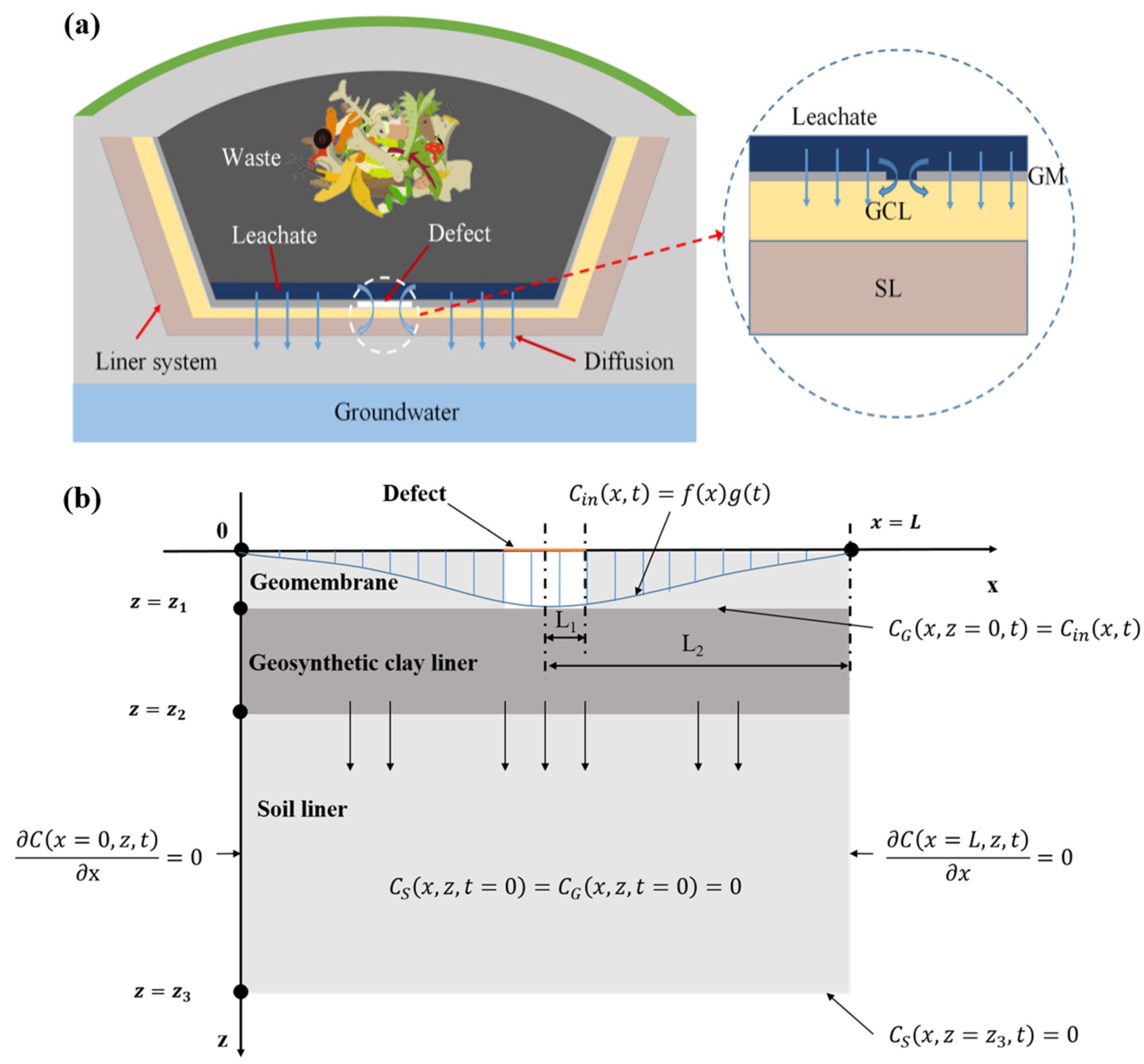
2. Mathematical Model

2.1. Basic Assumptions

As shown in Figure 1a, the composite liner system considered in this study comprises a GM, GCL, and SL (Figure 1b). The GM layer is assumed to be in a defective state, allowing direct contact with the leachate. In the context of the model, z₁ represents the thickness of the GM, z₂ represents the combined thickness of the GM and GCL, and z₃ represents the combined thickness of the GM, GCL, and SL. L₁ represents the width of the leak. The model is based on the following assumptions: (1) the flow of leachate within the liner is steady-state and obeys Darcy’s law; (2) migration of metal pollutants through the non-defective GM is neglected; (3) both the GCL and SL are assumed to be fully saturated and have uniform properties [32]; (4) the effects of convection, diffusion, adsorption, and degradation are considered; and (5) a linear, instantaneous, and reversible adsorption and first-order biodegradation reaction model are assumed.

2.2. Governing Equations and Boundary Conditions

Based on the above assumptions, the two-dimensional transport of pollutants in the GM/GCL/SL composite liner can be described by the equations of convection, diffusion, adsorption, and degradation.

For the GCL:

$${\mathrm{R}}_{\mathrm{d},\mathrm{G}}{\displaystyle \frac{\partial {\mathrm{C}}_{\mathrm{G}}}{\partial \mathrm{t}}}={\mathrm{D}}_{\mathrm{x},\mathrm{G}}{\displaystyle \frac{{\partial }^2{\mathrm{C}}_{\mathrm{G}}}{\partial {\mathrm{x}}^2}}+{\mathrm{D}}_{\mathrm{z},\mathrm{G}}{\displaystyle \frac{{\partial }^2{\mathrm{C}}_{\mathrm{G}}}{\partial {\mathrm{z}}^2}}-{\mathrm{v}}_{\mathrm{G}}{\displaystyle \frac{\partial {\mathrm{C}}_{\mathrm{G}}}{\partial \mathrm{z}}}-{\mathsf{\lambda }}_{\mathrm{G}}{\mathrm{C}}_{\mathrm{G}}$$

(1)

For the SL:

$${\mathrm{R}}_{\mathrm{d},\mathrm{S}}{\displaystyle \frac{\partial {\mathrm{C}}_{\mathrm{S}}}{\partial \mathrm{t}}}={\mathrm{D}}_{\mathrm{x},\mathrm{S}}{\displaystyle \frac{{\partial }^2{\mathrm{C}}_{\mathrm{S}}}{\partial {\mathrm{x}}^2}}+{\mathrm{D}}_{\mathrm{z},\mathrm{S}}{\displaystyle \frac{{\partial }^2{\mathrm{C}}_{\mathrm{S}}}{\partial {\mathrm{z}}^2}}-{\mathrm{v}}_{\mathrm{S}}{\displaystyle \frac{\partial {\mathrm{C}}_{\mathrm{S}}}{\partial \mathrm{z}}}-{\mathsf{\lambda }}_{\mathrm{S}}{\mathrm{C}}_{\mathrm{S}}$$

(2)

where C_i(i = G,S) represents the concentration of pollutants in the liner layer, which is a function of position and time; R_d,i represents the adsorption retardation factor of the i-th layer of the liner; D_x,i and D_z,i represent the diffusion coefficient in the x and z directions of the i-th layer, respectively; v_i is the convection coefficient in the liner layer; and λ_i represents the degradation constant of organic pollutants.

The expressions for the adsorption retardation factor (R_d) and degradation coefficient (λ) are, respectively:

$$R_d=1+{\displaystyle \frac{\rho K_d}{n}}$$

(3)

$$\lambda ={\displaystyle \frac{ln2}{t_{1/2}}}$$

(4)

where $\rho$ is the density of the liner, K_d is the distribution coefficient of the liner, and t_1/2 is the half-life of an organic pollutants.

Assuming the liner system has not been contaminated at the outset, the initial conditions of the liner system are:

$$C_S\left(x,z,t=0\right)=C_G\left(x,z,t=0\right)=0$$

(5)

where $C_S\left(x,z,t\right)$ represents the concentration of SL and $C_G\left(x,z,t\right)$ represents the concentration of GCL. The boundary conditions for the entrance of the GM defect can be represented by a concentration function in terms of width (x) and time (t):

$$C_M\left(x,z=0,t\right)=C_{in}\left(x,t\right)$$

(6)

where $C_M\left(x,z,t\right)$ represents the concentration of GM and the function $C_{in}\left(x,t\right)$ represents the concentration of the pollutant source, which is the product of a function $f\left(x\right)$ related to the width and a function g(t) related to time.

$$C_{in}\left(x,t\right)=f\left(x\right)g\left(t\right)$$

(7)

The lower boundary of the composite liner is assumed to be groundwater, a flushing boundary (i.e., zero concentration boundary):

$$C_S\left(x,z=z_3,t\right)=0$$

(8)

The left and right boundary condition of the model can be written as:

$${\displaystyle \frac{\partial C\left(x=0,z,t\right)}{\partial x}}=0$$

(9)

$${\displaystyle \frac{\partial C\left(x=L,z,t\right)}{\partial x}}=0$$

(10)

The concentration and flux at the interface between GCL and SL are equal, with expressions as follows:

$$C_G\left(x,z=z_1,t\right)=C_S\left(x,z=z_1,t\right)$$

(11)

$$-n_G{D}_G{\displaystyle \frac{\partial C_G\left(x,z=z_1,t\right)}{\partial z}}+n_G{v}_G{C}_G\left(x,z=z_1,t\right)=-n_S{D}_S{\displaystyle \frac{\partial C_S\left(x,z=z_1,t\right)}{\partial z}}+n_S{v}_S{C}_S\left(x,z=z_1,t\right)$$

(12)

where z₁ represents the thickness of GCL and $n_i(i=G,S)$ represents the porosity of the i-th layer. And, in the equations above, $n_G{v}_G=n_S{v}_S=v_d$, $v_d$ is Darcy’s velocity. Compared with previous studies, the governing equation of this study considers four kinds of contaminant transport behaviors in the liner and introduces the nonuniform concentration distribution function into the equation, which makes the mathematical expression of the problem clearer.

2.3. Analytical Solution

By applying the Laplace transform to the governing equations, the following equations can be obtained:

$$\overline{g}\left(s\right)=L\left(g\left(t\right)\right)={\int }_0^{+\mathrm{\infty }}g\left(t\right){\mathrm{e}}^{-st}\mathrm{d}t$$

(13)

For the GCL:

$$D_{x,G}{\displaystyle \frac{{\partial }^2{\overline{C}}_G\left(x,z,s\right)}{{\partial x}^2}}{+D}_{z,G}{\displaystyle \frac{{\partial }^2{\overline{C}}_G\left(x,z,s\right)}{{\partial z}^2}}-v_G{\displaystyle \frac{\partial {\overline{C}}_G\left(x,z,s\right)}{\partial z}}-\left(R_{d,G}s+{\lambda }_G\right){\overline{C}}_G\left(x,z,s\right)=0$$

(14)

For the SL:

$$D_{x,S}{\displaystyle \frac{{\partial }^2{\overline{C}}_S\left(x,z,s\right)}{{\partial x}^2}}{+D}_{z,S}{\displaystyle \frac{{\partial }^2{\overline{C}}_S\left(x,z,s\right)}{{\partial z}^2}}-v_S{\displaystyle \frac{\partial {\overline{C}}_S\left(x,z,s\right)}{\partial z}}-\left(R_{d,S}s+{\lambda }_S\right){\overline{C}}_S\left(x,z,s\right)=0$$

(15)

where ${\overline{C}}_G\left(x,z,s\right)$ and ${\overline{C}}_S\left(x,z,s\right)$ are the Laplace transform of $C_G\left(x,z,t\right)$ and $C_S\left(x,z,t\right)$, respectively. $s$ is the Laplace transform parameter.

Applying the Fourier series transform to the equation yields the following equation:

$$\widehat{F}\left(k\right)=F_c\left[f\left(x\right)\right]={\displaystyle \frac{2}{L}}{\int }_0^{L}f\left(x\right)\mathit{cos}\left({\displaystyle \frac{k\pi x}{L}}\right)\mathrm{d}x$$

(16)

For the GCL:

$$D_{z,G}{\displaystyle \frac{{\partial }^2{\widehat{\overline{C}}}_G\left(k,z,s\right)}{{\partial z}^2}}-v_G{\displaystyle \frac{\partial {\widehat{\overline{C}}}_G\left(k,z,s\right)}{\partial z}}-\left(R_{d,G}s+{\lambda }_G+{\displaystyle \frac{k^2{\pi }^2{D}_{x,G}}{L^2}}\right){\widehat{\overline{C}}}_G\left(k,z,s\right)=0$$

(17)

For the SL:

$$D_{z,S}{\displaystyle \frac{{\partial }^2{\widehat{\overline{C}}}_S\left(k,z,s\right)}{{\partial z}^2}}-v_S{\displaystyle \frac{\partial {\widehat{\overline{C}}}_S\left(k,z,s\right)}{\partial z}}-\left(R_{d,S}s+{\lambda }_S+{\displaystyle \frac{k^2{\pi }^2{D}_{x,S}}{L^2}}\right){\widehat{\overline{C}}}_S\left(k,z,s\right)=0$$

(18)

where ${\widehat{\overline{C}}}_G\left(k,z,s\right)$ and ${\widehat{\overline{C}}}_S\left(k,z,s\right)$ are the finite cosine form of ${\overline{C}}_G\left(x,z,s\right)$ and ${\overline{C}}_S\left(x,z,s\right)$, respectively. $k$ is the corresponding transform parameter.

Applying the same transform to both the boundary conditions and the equations, we obtain the following equations.

For the boundary conditions:

$${\widehat{\overline{C}}}_G\left(k,z=0,s\right)={\widehat{\overline{C}}}_{in}\left(k,s\right)=\widehat{f}\left(k\right)\overline{g}\left(s\right)$$

(19)

$${\widehat{\overline{\mathrm{C}}}}_{\mathrm{S}}\left(k,z=z_3,s\right)=0$$

(20)

For the equivalent interfacial concentration:

$${\widehat{\overline{C}}}_G\left(k,z=z_1,s\right)={\widehat{\overline{C}}}_S\left(k,z=z_1,s\right)$$

(21)

For the equivalent interfacial flux:

$$n_G{v}_G{\displaystyle \frac{\partial {\widehat{\overline{C}}}_G\left(k,z=z_1,s\right)}{\partial z}}=n_S{v}_S{\displaystyle \frac{\partial {\widehat{\overline{C}}}_S\left(k,z=z_1,s\right)}{\partial z}}$$

(22)

The homogeneous general solution of the concentration function can be written as:

$${\widehat{\overline{C}}}_i\left(k,z,s\right)=M_i{e}^{{\alpha }_{i}z}+N_i{e}^{{\beta }_{i}z}$$

(23)

where α_i, β_i can be expressed as:

$${\alpha }_i{,\beta }_i={\displaystyle \frac{\left\{v_i\pm \sqrt{v_i^2+4D_{z,i}\left(R_{d,i}s+{\lambda }_i+\frac{k^2{\pi }^2{D}_{x,i}}{L^2}\right)}\right\}}{2D_{z,i}}}$$

(24)

The matrix equation:

$$\left[\begin{array}{c}{M}_S\\ N_S\end{array}\right]=A\left[\begin{array}{c}{M}_{k,G}\\ N_{k,G}\end{array}\right]$$

(25)

Expression for coefficient $A$:

$$A={\displaystyle \frac{1}{{\alpha }_S{-\beta }_S}}\left[\begin{array}{cc}\left(\gamma {\alpha }_G-{\beta }_S\right)e^{{(\alpha }_G{-\alpha }_S)z_1}& \left(\gamma {\beta }_G-{\beta }_S\right)e^{{(\beta }_G{-\alpha }_S)z_1}\\ \left({\alpha }_S-\gamma {\alpha }_G\right)e^{{(\alpha }_G{-\beta }_S)z_1}& \left({\alpha }_S-\gamma {\beta }_G\right)e^{{(\beta }_G{-\beta }_S)z_1}\end{array}\right]$$

(26)

Expression for coefficient γ:

$$\gamma ={\displaystyle \frac{n_G{D}_{z,G}}{n_S{D}_{z,S}}}$$

(27)

Coefficient $A$ in matrix form is expressed as:

$$A=\left[\begin{array}{cc}{A}_{11}& A_{12}\\ A_{21}& A_{22}\end{array}\right]$$

(28)

Translation of the concentration expression when $z$ is zero is as follows:

$${\widehat{\overline{C}}}_G\left(k,z=0,s\right)=M_G+N_G=\widehat{f}\left(k\right)\overline{g}\left(s\right)$$

(29)

Translation of the concentration expression when $z$ equals $z_3$ is as follows:

$${\widehat{\overline{C}}}_S\left(k,z=z_3,s\right)=M_S{e}^{{\alpha }_S{z}_3}+N_S{e}^{{\beta }_S{z}_3}=0$$

(30)

The correlation between concentration expression and matrix form is as follows:

$$\left[\begin{array}{c}{M}_G\\ N_G\end{array}\right]=\left[\begin{array}{c}{\displaystyle \frac{{-A}_{12}{e}^{{\alpha }_s{z}_3}-A_{22}{e}^{{\beta }_s{z}_3}}{A_{11}{e}^{{\alpha }_S{z}_3}{-A}_{12}{e}^{{\alpha }_s{z}_3}+A_{21}{e}^{{\beta }_s{z}_3}-A_{22}{e}^{{\beta }_s{z}_3}}}\\ {\displaystyle \frac{A_{11}{e}^{{\alpha }_s{z}_3}+A_{21}{e}^{{\beta }_s{z}_3}}{A_{11}{e}^{{\alpha }_S{z}_3}{-A}_{12}{e}^{{\alpha }_s{z}_3}+A_{21}{e}^{{\beta }_s{z}_3}-A_{22}{e}^{{\beta }_s{z}_3}}}\end{array}\right]\widehat{f}\left(k\right)\overline{g}\left(s\right)$$

(31)

Applying the inverse transform to the equation, the solution for the original problem is finally obtained.

For the GCL (0 < z₁ ≤ z ≤ z₂):

$${\overline{C}}_G\left(x,z,s\right)={\displaystyle \frac{1}{2}}{(M}_G{e}^{{\alpha }_G\left(k=0,s\right)z}+N_G{e}^{{\beta }_G\left(k=0,s\right)z})+\sum _{k=1}^{+\mathrm{\infty }}{(M}_{k, G}{e}^{{\alpha }_{G}z}+N_{k, G}{e}^{{\beta }_{G}z})\mathit{cos}\left({\displaystyle \frac{k\pi x}{L}}\right)$$

(32)

For the SL (z₂ ≤ z ≤ z₃):

$${\overline{C}}_S\left(x,z,s\right)={\displaystyle \frac{1}{2}}{(M}_S{e}^{{\alpha }_S(k=0,s)z}+N_S{e}^{{\beta }_S(k=0,s)z})+\sum _{k=1}^{+\mathrm{\infty }}{(M}_{k, S}{e}^{{\alpha }_{S}z}+N_{k, S}{e}^{{\beta }_{S}z})\mathit{cos}\left({\displaystyle \frac{k\pi x}{L}}\right)$$

(33)

Since the solution presented in Equations (32) and (33) is written in terms of s, which is the Laplace complex number, this study adopts the Talbot’s version algorithm [33] to solve the equations to obtain the solution in the real time domain.

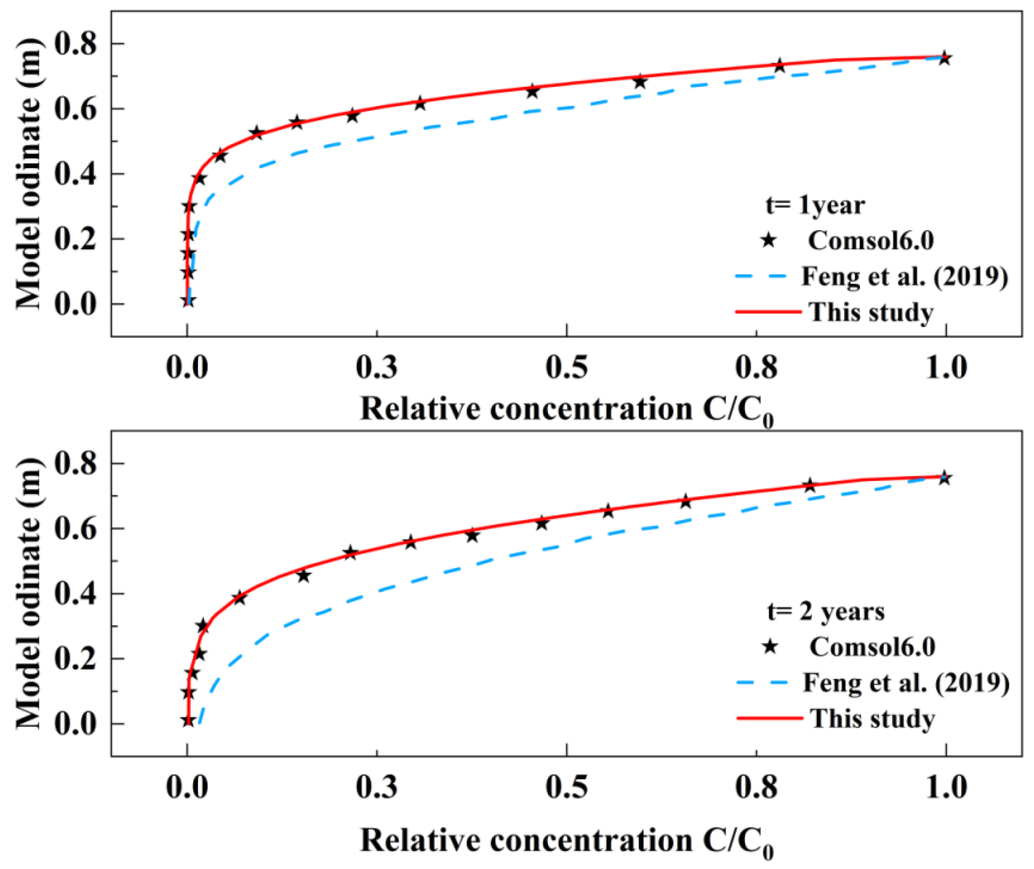
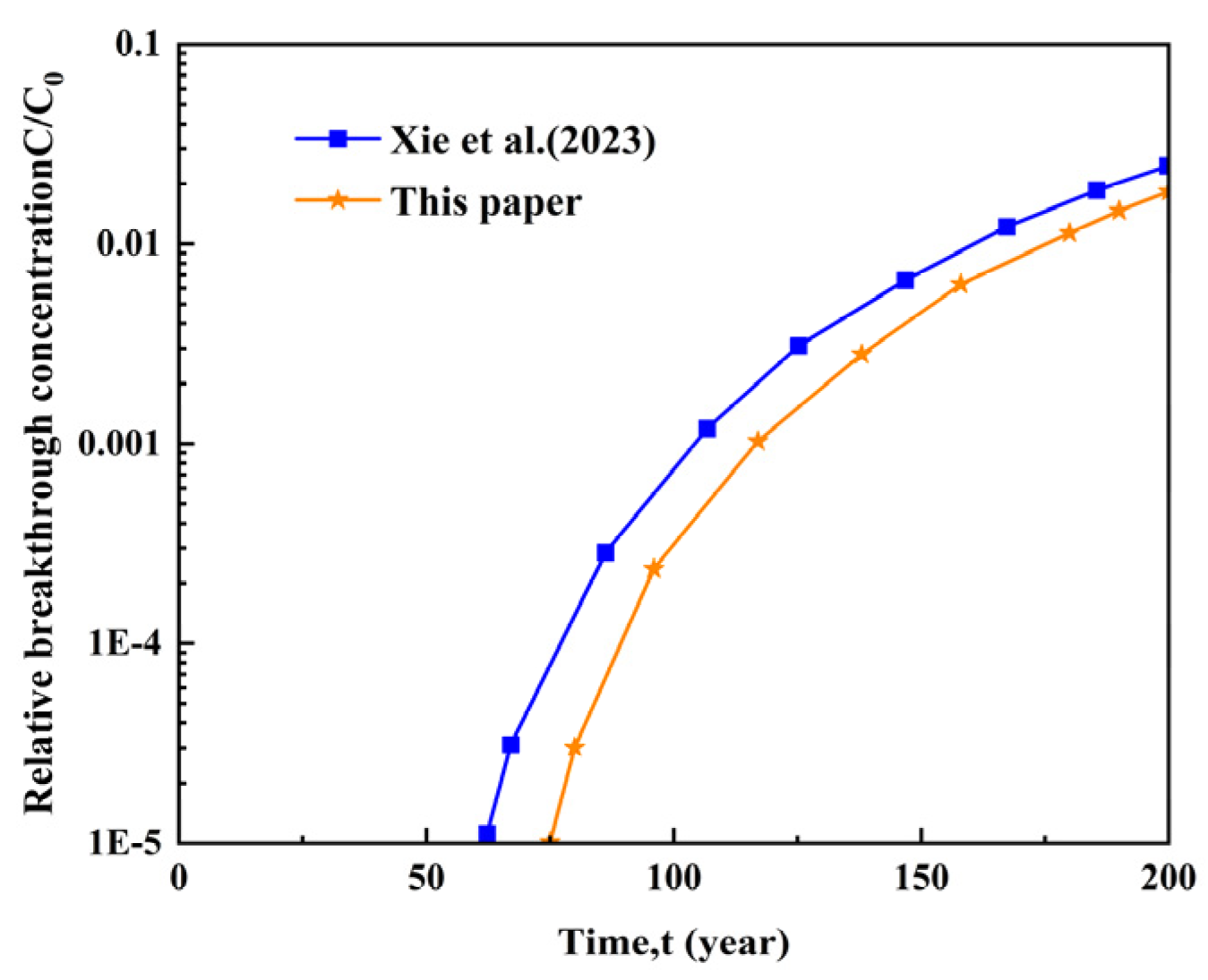
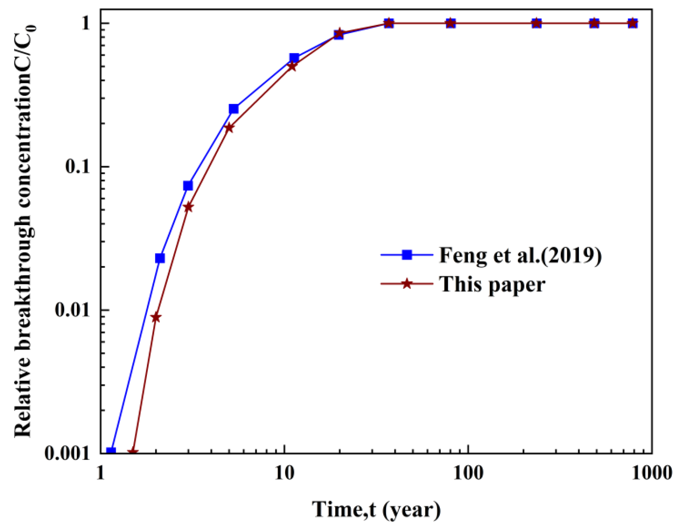
3. Model Verification

To validate the effectiveness and reasonableness of the analytical solution in this study, an analytical solution for solute transport in double-layered finite porous media was chosen as a benchmark. The liner system model used in this study consists of a 1.5 mm GM, a 1 cm GCL, and a 75 cm SL. The analytical solution was validated using the one-dimensional analytical solution provided by Feng et al. [24]. In this study, the water head was set at 0.3 m, and the other coefficients are provided in

Table 1. Parameters used in this study [30,32,34,35].

Parameter	Pollutants	GM	GCL	SL
Thickness, L (m)	-	0.0015	0.01	0.75
Porosity, n	-	-	0.7	0.3
Dry density, ρd (g/cm3)	-	-	0.79	1.62
Hydraulic conductivity, k (m/s)	-	-	0.5 × 10−10	1 × 10−7
Effective diffusion coefficient, D (m2 /s)	-	3 × 10−13	3 × 10−10	8 × 10−10
	Zn2+	6 × 10−15	7.15 × 10−10	8.9 × 10−10
	TOL	3 × 10−13	3 × 10−10	8 × 10−10
Distribution coefficient, Kd (mL/g)	-	0	0	0
Partition coefficient, Kg	-	100	-	-

below.

The results, as shown in Figure 2, indicate that, at the two-year mark, the pollutant concentration calculated by the model shows some differences from the data in the reference literature at distances further from the GCL. This discrepancy is attributed to the consideration of pollutant degradation within the liner in this study, resulting in lower pollutant concentrations at greater distances compared to the reference literature.

To further verify the model’s accuracy in two dimensions, COMSOL Multiphysics 6.0 was used to compare the concentrations of pollutants after one year and two years. The results demonstrate a high degree of consistency between the COMSOL model and the analytical solution utilized in this study, providing robust verification for these research outcomes. The parameters used are as follows.

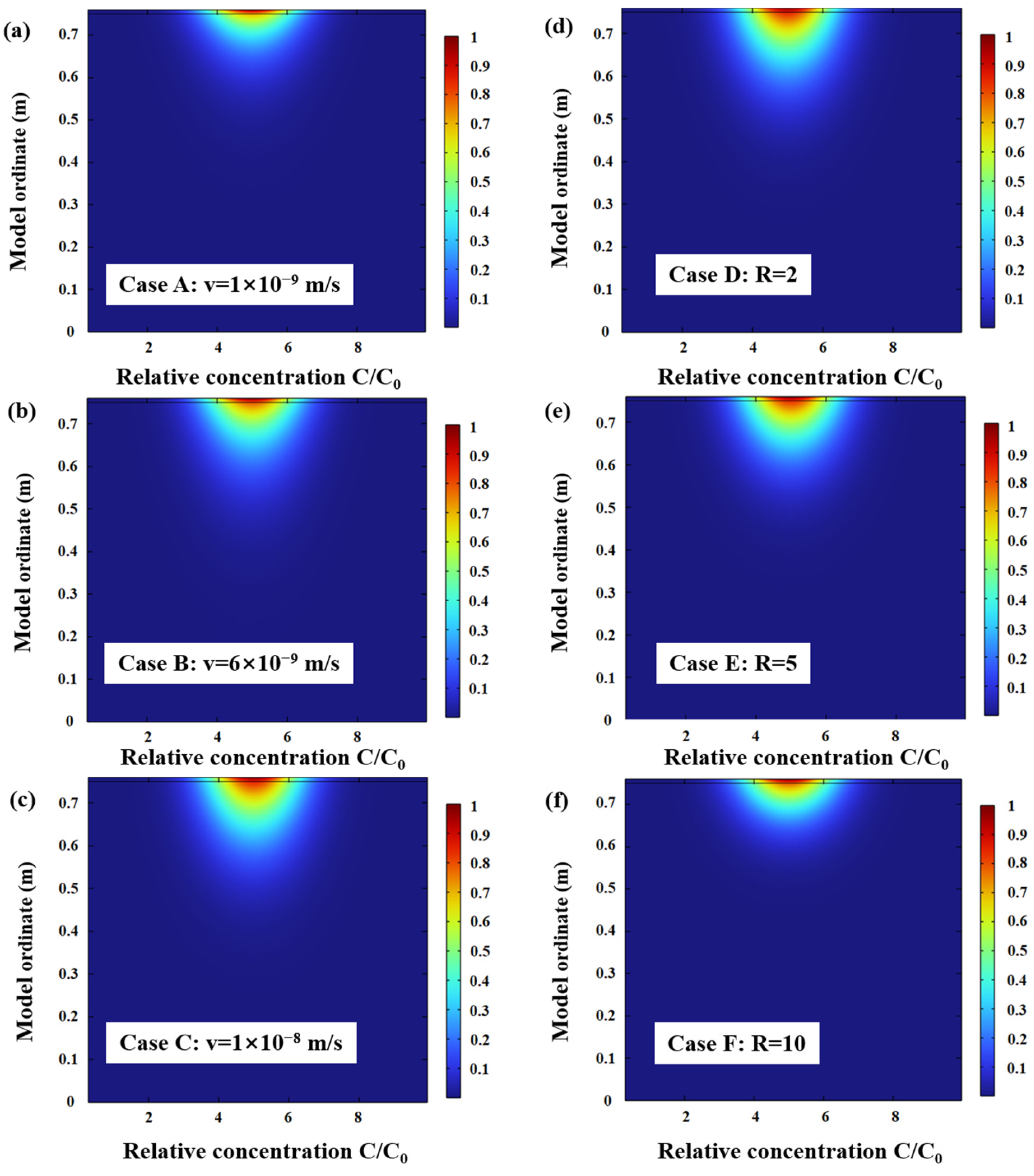
4. Uneven Distribution of Pollutant Concentrations at the Liner Leak Points

Damage to the GM in the liner system results in a nonuniform distribution of pollutant concentrations during the subsequent transport through the liner. As shown in Figure 3, the diffusion coefficient of heavy metal pollutants in the GM is significantly smaller than that in the defective areas. Therefore, this study employs distinct concentration functions for heavy metal pollutants and organic pollutants. Specifically, for heavy metal ion pollutants, this study uses the concentration function proposed by Xie et al. [30].

$$C=C_0{K}_g$$

(34)

Here, the contaminant concentration in the leachate is assumed as a constant $C_0$ and $K_g$ is the partition coefficient, which is the ratio of pollutant concentration in leachate to that in the geomembrane. Since heavy metal ions cannot degrade in the liner, the control equation can be simplified accordingly:

$$R_{d,i}{\displaystyle \frac{\partial C_i}{\partial t}}=D_{x,i}{\displaystyle \frac{{\partial }^2{C}_i}{\partial x^2}}+D_{z,i}{\displaystyle \frac{{\partial }^2{C}_i}{\partial z^2}}-v_i{\displaystyle \frac{\partial C_i}{\partial z}}$$

(35)

For organic pollutants, the concentration distribution can be more accurately described using the standard Gaussian function, as mentioned by Ding et al. [34], to provide a more precise description of the concentration distribution.

$$\mathrm{C}=C_{in,max}\times exp({-(x-\mu )}^2/2{\sigma }^2)$$

(36)

where C_in,max represents the largest concentration of the pollutant source, μ represents the abscissa of C_in,max, and σ represents the distribution range of the high concentration.

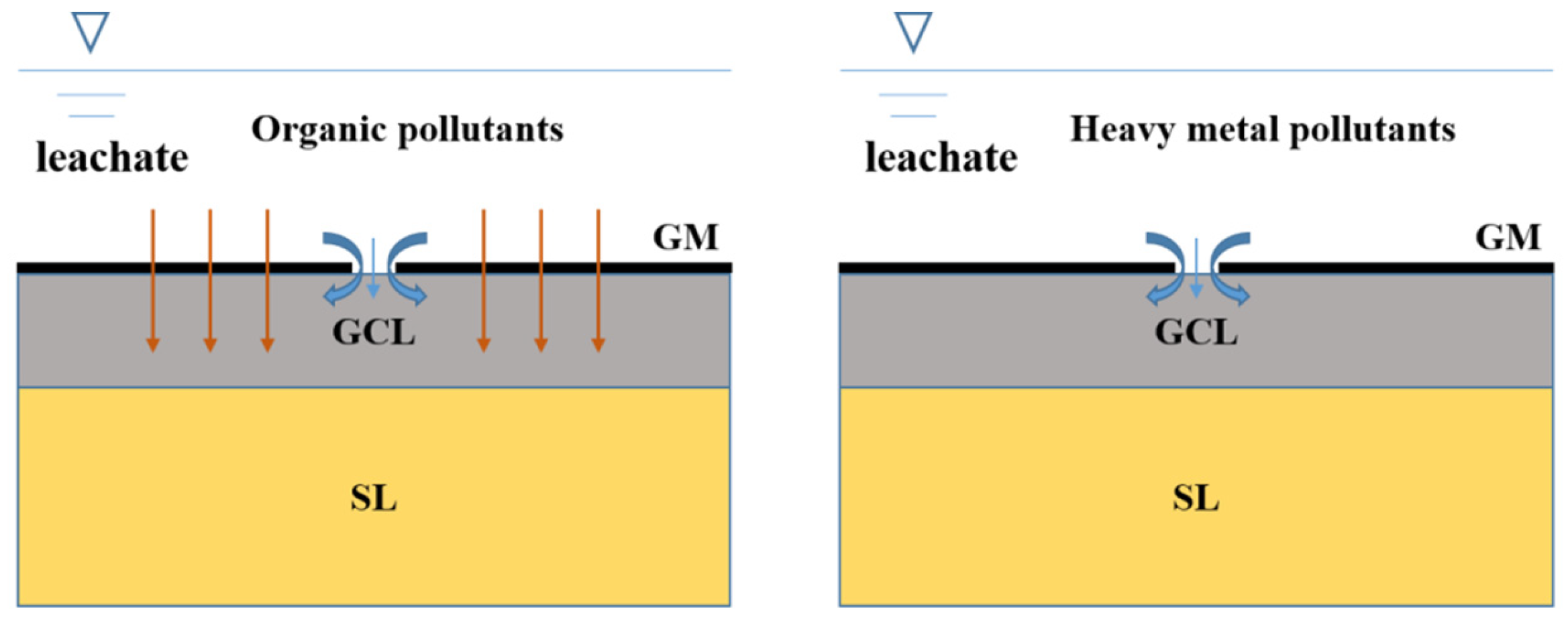
5. Pollution Prevention Performance of Composite Liner Systems

5.1. Heavy Metal Ion Zinc (Zn²⁺)

Zn²⁺ is a common heavy metal pollutant found in leachate. Therefore, this heavy metal ion was selected for analysis. The only significant pathway for contaminant transport is through defects in the geomembrane [35]. Using Equation (34) as the initial concentration distribution function for Zn²⁺, Figure 4 presents the breakthrough concentration of Zn²⁺ within the liner system over different time intervals. As time elapses, the breakthrough concentration of Zn²⁺ in the liner increases. However, the results of this paper are consistently slightly lower than the results of Xie et al. [36]. This is caused by the differences in concentration distribution functions. As time increases, the deviation in breakthrough concentration gradually decreases. This indicates that this function can be used to describe the transport of heavy metal ions.

5.2. Organic Pollutant Toluene (TOL)

Leachate typically contains a substantial quantity of organic pollutants. If these organic pollutants were to leak through the GM and migrate through the composite liner system, they could cause significant damage to the soil and groundwater. Using Equation (36) as the initial concentration distribution function, therefore, this study focuses on TOL as a representative organic pollutant to investigate its migration within the composite liner system, as illustrated in Figure 5.

Organic pollutants, such as TOL, exhibit a higher diffusion capacity within the liner compared to heavy metal pollutants, making them more likely to penetrate the GM. Due to its faster diffusion rate within the liner system, the breakthrough time of TOL is less than the time of Zn²⁺. When the migration time is short, there is a subtle difference between this study and Feng et al. [24]. However, after 20 years, the breakthrough concentration of the two become basically consistent. These findings underscore that that function can be used to describe the transport of organic pollutants.

6. Results and Discussion

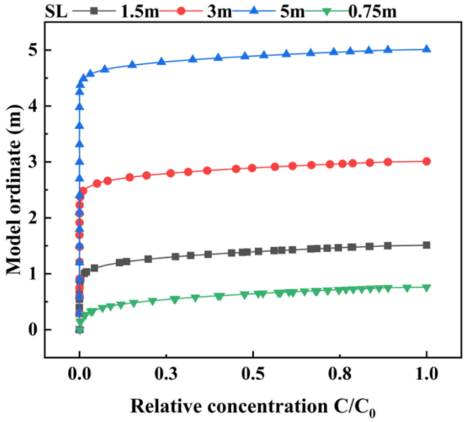
For the GM/GCL/SL composite liner system, this study analyzed the effects of changes in SL thickness, diffusion coefficients of GCL and SL, hydraulic conductivity, and adsorption hindrance factors on the migration of pollutants within the liner layer. The parameters of the reference model are provided in Table 1. When one parameter is changed, the other parameters are kept constant.

6.1. SL Thickness

The thickness of the SL plays a crucial role in both the migration time of contaminants within the liner and the economic cost of the liner system. Determining the optimal SL thickness is crucial for the efficient design of landfill liner systems, balancing both environmental protection and economic considerations. To investigate this, SL thicknesses of 0.75 m, 1.5 m, 3 m, and 5 m were selected for further research and analysis.

As illustrated in Figure 6, increasing the SL thickness from 0.75 m to 1.5 m does not significantly impact the concentration of contaminants near the GM and GCL. Instead, the concentration curve shifts upward, indicating an increase in the thickness at which the concentration becomes zero. However, as the SL thickness continues to increase beyond 1.5 m, the concentration of contaminants near the GM remains relatively constant. For SL thicknesses of 0.75 m, 1.5 m, 3 m, and 5 m, the concentrations are essentially identical, suggesting that the SL thickness does not significantly affect contaminant migration within the liner system.

These findings align with the work of Pandey and Babu [37], who reported that contaminant diffusion rates stabilize beyond a certain liner thickness due to the diminishing permeability and adsorption capacity of the materials used. In contrast, Brown and Thomas [38] found that, for highly volatile organic compounds, even slight increases in liner thickness could significantly reduce diffusion rates, although their study focused on specialized industrial waste applications. Additionally, economic analyses by Sarkar et al. [39] suggest that the cost–benefit ratio becomes unfavorable as SL thickness exceeds the optimal range, with increased material and construction costs not justifying the marginal gains in containment efficacy. This economic perspective is crucial for environmental engineering, where cost efficiency must be balanced with environmental protection.

In practice, our results suggest that there is an optimal thickness for the soil layer (SL) that balances the effectiveness of pollutant containment and material usage. Beyond this optimal thickness, increases in SL do not significantly improve the performance of the liner system in terms of contaminant migration. Therefore, selecting an appropriate SL thickness is crucial to achieve a balance between environmental protection and cost efficiency, ensuring that the liner provides adequate containment without unnecessary material overuse.

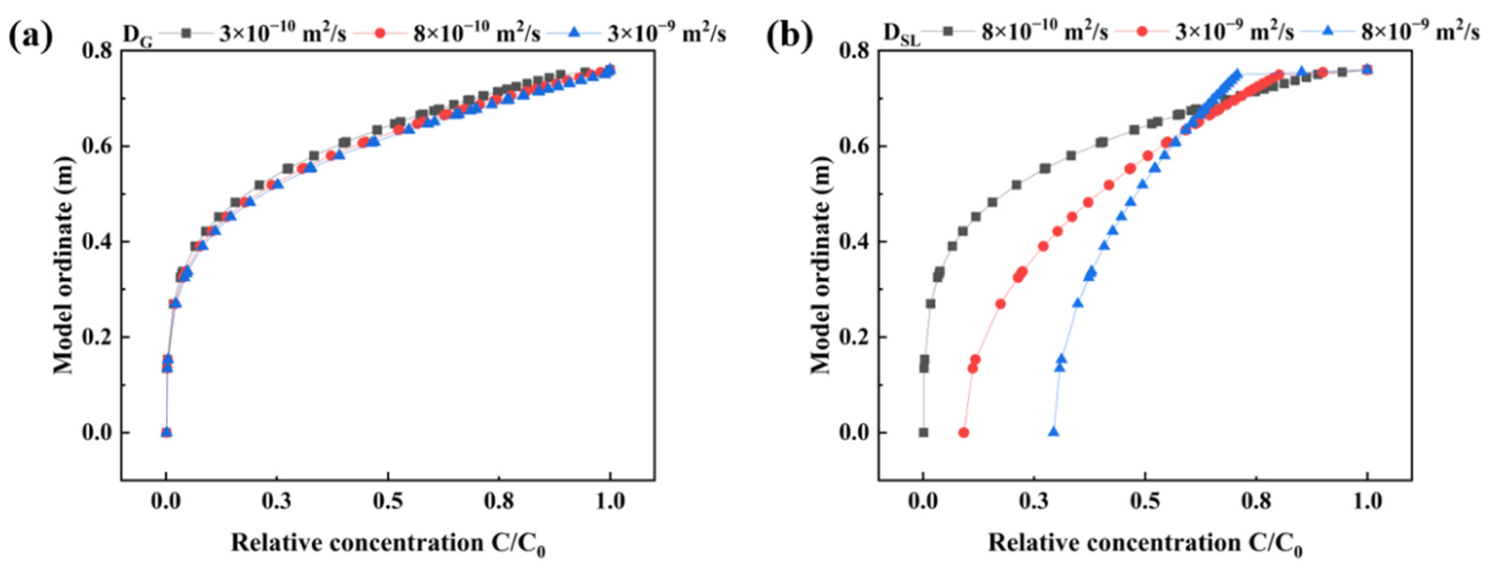
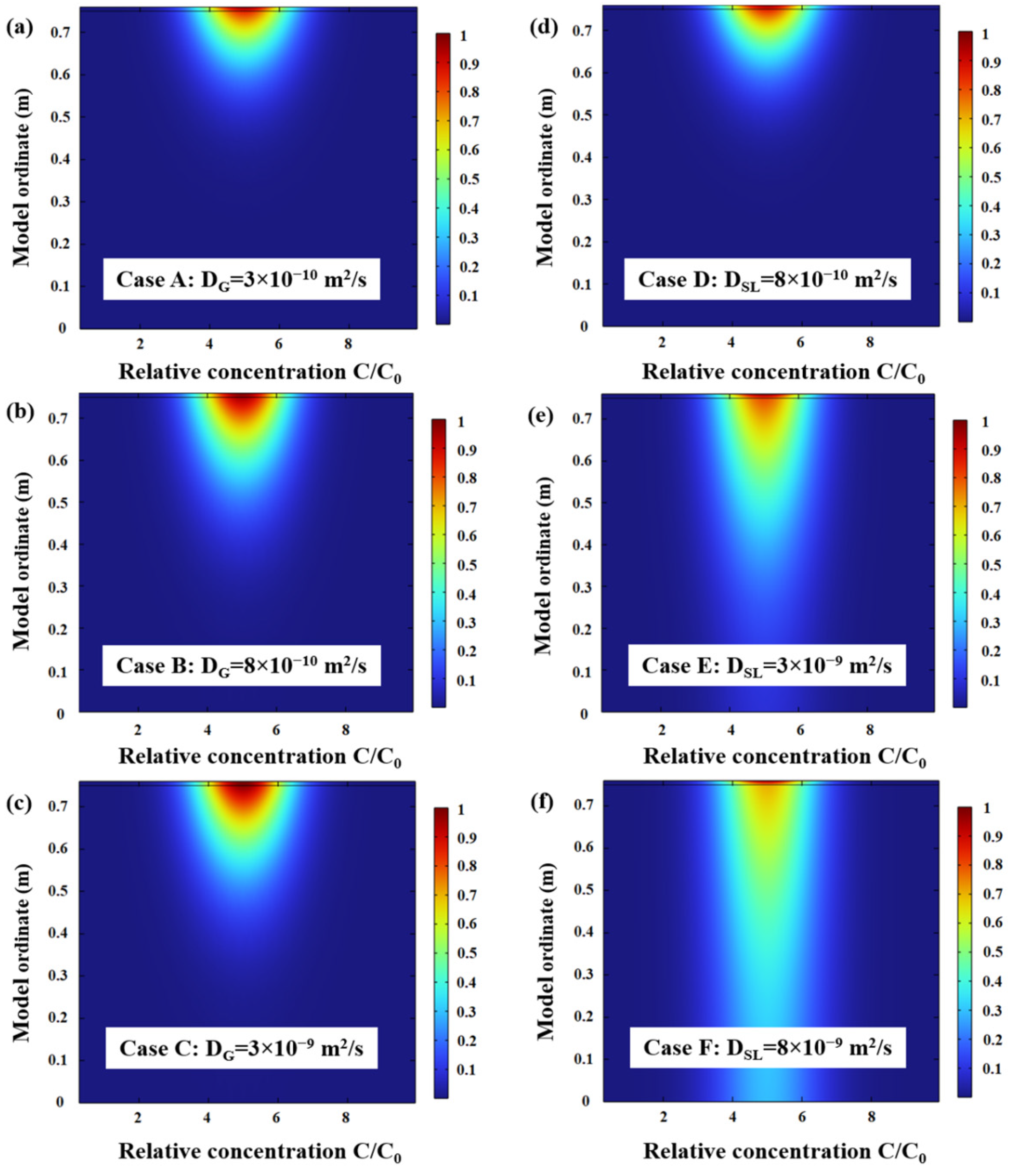
6.2. Diffusion Coefficient

The diffusion coefficient is a pivotal factor in understanding contaminant migration within a liner, reflecting the varied material properties of GCL and SL. This study investigated the impacts of different diffusion coefficients for GCL and SL on contaminant dispersion. Specifically, diffusion coefficients for GCL were considered at 3 × 10⁻¹⁰ m²/s, 8 × 10⁻¹⁰ m²/s, and 3 × 10⁻⁹ m²/s; for SL, the coefficients were 8 × 10⁻¹⁰ m²/s, 3 × 10⁻⁹ m²/s, and 8 × 10⁻⁹ m²/s.

Figure 7a,b analyze the effects of these varying diffusion coefficients on contaminant migration within the composite liner. Figure 8 simulates pollutant concentrations, with Figure 8a–c highlighting the impacts of varying GCL diffusion coefficients and Figure 8d–f showcasing those for SL. Variations in the GCL diffusion coefficient from 3 × 10⁻¹⁰ m²/s to 3 × 10⁻⁹ m²/s demonstrate a measurable influence on contaminant migration. The concentration profiles indicate that, as the diffusion coefficient increases, the relative concentration of contaminants near the GM also increases. However, due to the relatively thin nature of GCL layers, this impact remains moderate. The contour plots reveal steeper concentration gradients with higher diffusion coefficients, indicating more rapid contaminant migration through the GCL. Conversely, changes in the SL diffusion coefficient result in a more pronounced increase in contaminant concentrations near the GCL interface. As the diffusion coefficient of SL increases from 8 × 10⁻¹⁰ m²/s to 8 × 10⁻⁹ m²/s, there is a significant increase in the spread of contaminants. This is attributed to the greater thickness and permeability of the SL compared to the GCL. The broader spread of contaminants with higher SL diffusion coefficients underscores the stronger influence of SL on contaminant migration within the liner system.

Xie et al. [21] found that increases in the diffusion coefficient in similar composite liners lead to significantly enhanced migration rates of hydrophobic organic contaminants, particularly when the liners exhibit higher permeability. Moreover, studies by Anisimov et al. [40] further corroborate that the material characteristics of SL can amplify the diffusion effects due to its greater thickness and the interaction of multiple soil layers. Interestingly, the discrepancies between the diffusion effects in GCL and SL highlighted in this study are also reflected in the work of Majumder et al. [41], who observed that diffusion in geosynthetic layers tends to stabilize more rapidly than in soil layers, primarily due to the structured nature of geosynthetics compared to the heterogeneous composition of soil. The results suggest that careful consideration of diffusion properties is essential for designing effective composite liner systems. Optimizing the diffusion coefficients for both GCL and SL can significantly enhance the containment performance of these systems.

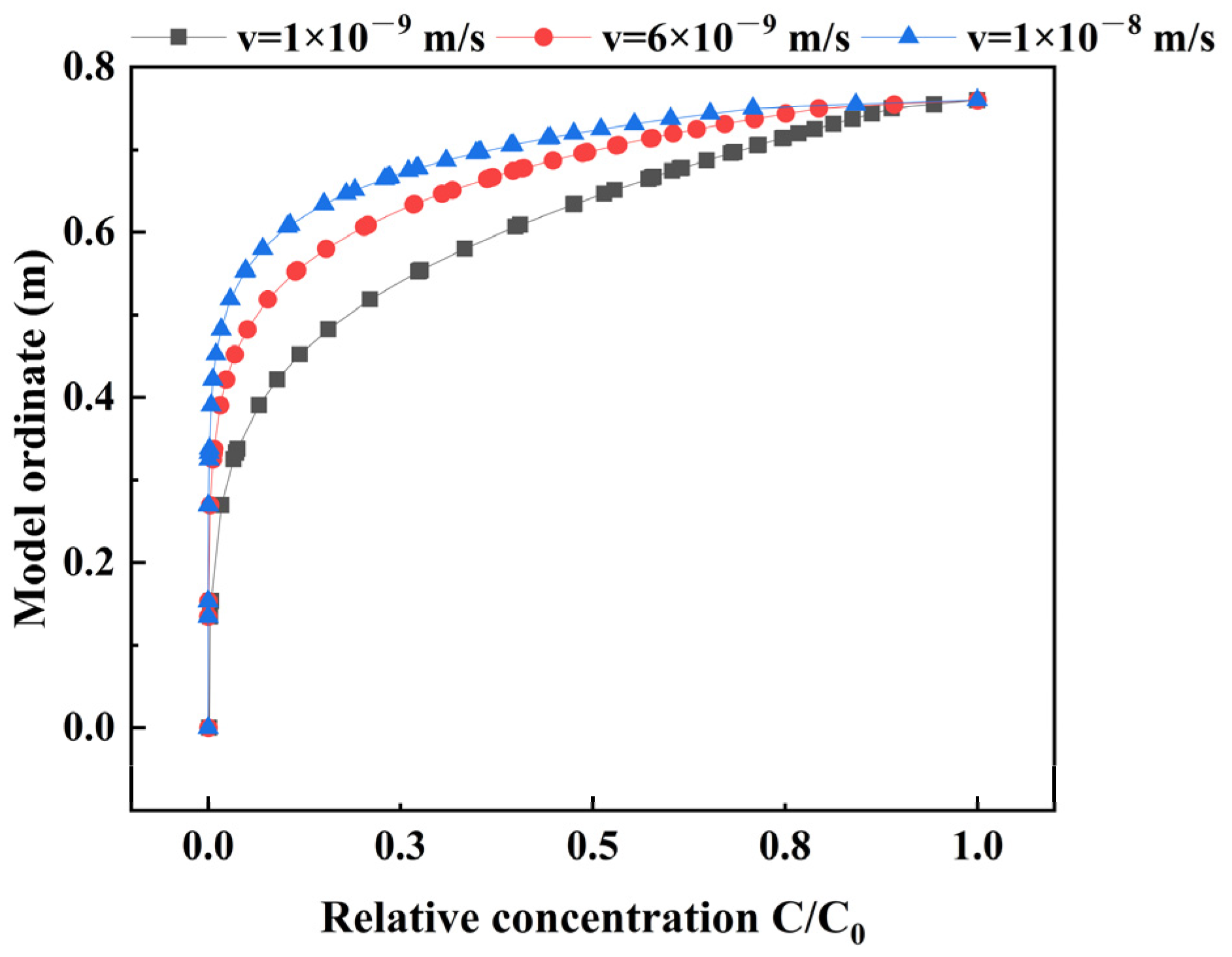
6.3. Advection Velocity

The advection velocity plays a pivotal role in contaminant transport within liner systems, significantly impacting both GCL and SL layers. To elucidate the role of convection in contaminant migration, advection velocities of 1 × 10⁻⁹ m/s, 6 × 10⁻⁹ m/s, and 1 × 10⁻⁸ m/s were selected for analysis.

Figure 9 demonstrates that, as the advection velocity increases, the diffusion distance of contaminants gradually increases as they penetrate deeper into the liner. Specifically, Figure 10a–c illustrate the effects of these varying advection velocities. When the advection velocity reaches 1 × 10⁻⁸ m/s, the contaminant diminishes to approximately zero after migrating 0.55 m. Conversely, with an advection velocity of 1 × 10⁻⁹ m/s, the concentration decreases to zero after migrating 0.3 m. Clearly, the advection velocity significantly influences contaminant migration within the liner. Thus, in the practical design of landfill projects, careful consideration of the advection velocity is imperative to ensure the rational adjustment of liner materials and design. Yeo et al. [42] demonstrated that higher advection velocity significantly accelerates contaminant migration in synthetic liners due to enhanced advection processes. Similarly, research by Ameijeiras-Mariño et al. [43] in soil liners found that increases in advection velocity could reduce the residence time of contaminants within the liner, potentially compromising the containment effectiveness unless compensated by other design modifications. In practical applications, especially in landfill project design, it is crucial to consider the advection velocity to ensure the effective containment of contaminants by making appropriate adjustments to liner materials and system designs.

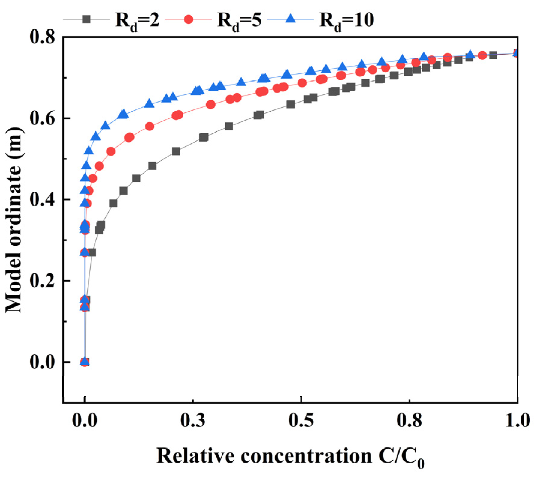
6.4. Adsorption Retardation Factor

The adsorption retardation factor has a certain effect on impeding the rapid migration of contaminants within the liner layer. Adsorption retardation factors of 2, 5, and 10 were employed to simulate contaminant migration within the composite liner. Figure 10d–f illustrate the effects of adsorption retardation factor.

Figure 11 demonstrates the impact of these differing adsorption retardation factors on contaminant migration. As the adsorption retardation factor increases, the migration of contaminants decelerates. For instance, with a retardation factor of 2, the contaminant concentration decreases to zero after migrating 0.55 m within the liner layer. When the retardation factor is increased to 5, the concentration drops to zero after migrating 0.35 m. Furthermore, with a retardation factor of 10, the concentration reaches zero after migrating 0.25 m. This indicates that, as the adsorption retardation factor increases, the migration of contaminants slows down, although the retarding effect on the contaminants decreases accordingly.

These findings align with the observations of Chrysikopoulos et al. [44], who reported that the sorption effect significantly slows down pollutant migration. Additionally, studies by Lin and Yeh [45] corroborate that the larger the adsorption factor, the shorter the migration distance of pollutants. Therefore, if the adsorption retardation effect in the liner is significant, it is essential to incorporate the retardation factor into the mathematical model to accurately predict contaminant behavior.

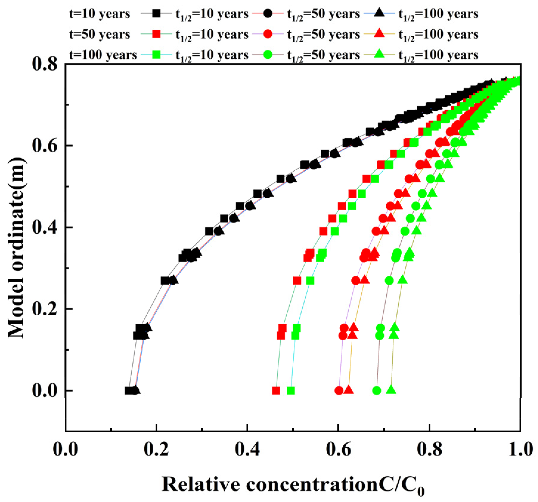
6.5. Degradation Coefficient

Figure 12 illustrates the effect of the degradation coefficient of organic pollutants in SL, considering different half-lives set at 10 years, 50 years, and 100 years. The concentrations are compared for migration times of 10 years, 50 years, and 100 years.

When the migration time (t) is 10 years, the three concentration curves exhibit minimal differences. However, as the half-life decreases, the pollutant concentration also decreases. At t = 50 years, significant differences between the concentration curves emerge, with the concentration under the 10-year half-life scenario notably lower than that under the 50-year and 100-year scenarios. The concentration is highest under the 100-year half-life scenario. As t increases to 100 years, these concentration differences become even more pronounced.

The results indicate that the half-life of organic pollutants in the composite liner system significantly affects the concentration of pollutants within the liner. However, due to the long degradation time and minimal degradation of organic pollutants over a short period, variations in degradation coefficients have a limited effect on preventing the migration of pollutants in the composite liner. Feng et al. [46] and Peng et al. [47] also proposed that, when the half-life is short, the degradation effect is more pronounced. However, when the half-life is long, the degradation effect can be neglected in the short term. Understanding the degradation coefficients and their impact on pollutant migration is crucial for designing effective composite liner systems. While short-term degradation may not significantly influence pollutant concentration, long-term degradation can substantially reduce contaminant levels, enhancing the liner’s protective performance.

7. Limitations

One fundamental limitation of the proposed model in this study is its assumption of uniformity and isotropy within the same liner layer. This simplification overlooks the potential for heterogeneity and anisotropy, which are commonly observed in real-world landfill systems. Additionally, the model simplifies convection to only the vertical direction to enable an analytical solution, focusing on gravity-driven vertical leachate migration. However, this excludes horizontal flow and associated hydraulic dispersion, which may influence pollutant transport in certain scenarios. Furthermore, the model assumes diffusion anisotropy in the liner materials, attributing higher horizontal diffusion coefficients compared to vertical diffusion coefficients due to the preferential alignment of particles and compaction-induced anisotropy in clay and soil layers. This assumption aligns with observed structural characteristics of GCL and SL but may not fully capture all real-world anisotropic behaviors.

Another limitation is the exclusion of macroscopic features such as cracks or joints within the liner system, which can serve as preferential paths for the migration of contaminants. While the model assumes a defective GM, it does not specifically simulate the complex flow dynamics that can occur around these defects, nor does it consider the potential for repair or mitigation measures that might be applied in practical settings.

8. Summary

Considering the uneven distribution of pollutants behind the GM in composite liners, a two-dimensional model was developed to investigate the contaminant migration behavior. This model accounts for convection, diffusion, adsorption, and degradation processes within the liner and has been verified through the one-dimensional analytical solution and the two-dimensional numerical results computed using the COMSOL model. Analysis of key factors led to the following conclusions:

(1)

The concentration distributions of organic pollutants and metal pollutants in the liner differ to some extent and, using the same function to describe these distributions can affect the extent of contamination. Employing two distinct concentration distribution functions enhances accuracy.

(2)

Compared to alternative analytical solutions and COMSOL verification results, the proposed analytical solution demonstrates a satisfactory level of accuracy, effectively describing pollutant migration processes in composite liners.

(3)

The concentration curve of pollutants is more sensitive to changes in the diffusion coefficient of SL than to changes in the diffusion coefficient of GCL. Specifically, as the diffusion coefficient of SL increases from 8 × 10⁻¹⁰ m²/s to 8 × 10⁻⁹ m²/s, the concentration curves intersect. However, when the diffusion coefficient of GCL increases from 3 × 10⁻¹⁰ m²/s to 3 × 10⁻⁹ m²/s, the concentration distribution curve of pollutants exhibits minimal changes, indicating comparable pollution prevention capabilities in both scenarios.

References

1. Gómez-García, R.; Campos, D.A.; Aguilar, C.N.; Madureira, A.R.; Pintado, M. Valorisation of food agro-industrial by-products: From the past to the present and perspectives. J. Environ. Manag. 2021, 299, 113571. [Google Scholar] [CrossRef] [PubMed]
2. Ghosh, A.; Kumar, S.; Das, J. Impact of leachate and landfill gas on the ecosystem and health: Research trends and the way forward towards sustainability. J. Environ. Manag. 2023, 336, 117708. [Google Scholar] [CrossRef] [PubMed]
3. Ling, X.; Chen, W.; Schollbach, K.; Brouwers, H. Low permeability sealing materials based on sewage, digestate and incineration industrial by-products in the final landfill cover system. Constr. Build. Mater. 2024, 412. [Google Scholar] [CrossRef]
4. Qian, Y.; Hu, P.; Lang-Yona, N.; Xu, M.; Guo, C.; Gu, J.-D. Global landfill leachate characteristics: Occurrences and abundances of environmental contaminants and the microbiome. J. Hazard. Mater. 2023, 461, 132446. [Google Scholar] [CrossRef]
5. Sobral, B.; Samper, J.; Montenegro, L.; Mon, A.; Guadaño, J.; Gómez, J.; Román, J.S.; Delgado, F.; Fernández, J. 2D model of groundwater flow and total dissolved HCH transport through the Gállego alluvial aquifer downstream the Sardas landfill (Huesca, Spain). J. Contam. Hydrol. 2024, 265, 104370. [Google Scholar] [CrossRef]
6. Wu, L.; Zhan, L.; Lan, J.; Chen, Y.; Zhang, S.; Li, J.; Liao, G. Leachate migration investigation at an unlined landfill located in granite region using borehole groundwater TDS profiles. Eng. Geol. 2021, 292, 106259. [Google Scholar] [CrossRef]
7. Zhang, J.; Zhang, J.-M.; Xing, B.; Liu, G.-D.; Liang, Y. Study on the effect of municipal solid landfills on groundwater by combining the models of variable leakage rate, leachate concentration, and contaminant solute transport. J. Environ. Manag. 2021, 292, 112815. [Google Scholar] [CrossRef]
8. Abiriga, D.; Vestgarden, L.S.; Klempe, H. Groundwater contamination from a municipal landfill: Effect of age, landfill closure, and season on groundwater chemistry. Sci. Total. Environ. 2020, 737, 140307. [Google Scholar] [CrossRef]
9. Shu, S.; Zhu, W.; Shi, J. A new simplified method to calculate breakthrough time of municipal solid waste landfill liners. J. Clean. Prod. 2019, 219, 649–654. [Google Scholar] [CrossRef]
10. Teng, C.; Zhou, K.; Peng, C.; Chen, W. Characterization and treatment of landfill leachate: A review. Water Res. 2021, 203, 117525. [Google Scholar] [CrossRef]
11. Wijekoon, P.; Koliyabandara, P.A.; Cooray, A.T.; Lam, S.S.; Athapattu, B.C.; Vithanage, M. Progress and prospects in mitigation of landfill leachate pollution: Risk, pollution potential, treatment and challenges. J. Hazard. Mater. 2022, 421, 126627. [Google Scholar] [CrossRef] [PubMed]
12. Trauger, R.; Tewes, K. Design and Installation of a State-of-the-Art Landfill Liner System in Geosynthetic Clay Liners; CRC Press: Boca Raton, FL, USA, 2020; pp. 175–181. [Google Scholar]
13. Li, D.; Zhao, H.; Tian, K. Hydraulic conductivity of bentonite-polymer geosynthetic clay liners to aggressive solid waste leachates. Geotext. Geomembr. 2024, 52, 900–911. [Google Scholar] [CrossRef]
14. Guan, C.; Xie, H.; Wang, Y.; Chen, Y.; Jiang, Y.; Tang, X. An analytical model for solute transport through a GCL-based two-layered liner considering biodegradation. Sci. Total. Environ. 2014, 466, 221–231. [Google Scholar] [CrossRef]
15. Li, T.; Sun, D.; Chen, Z.; Wang, L. Semi-analytical solution for two-dimensional contaminant transport through composite liner with strip defects. Constr. Build. Mater. 2024, 440, 137404. [Google Scholar] [CrossRef]
16. Zainab, B.; Wireko, C.; Li, D.; Tian, K.; Abichou, T. Hydraulic conductivity of bentonite-polymer geosynthetic clay liners to coal combustion product leachates. Geotext. Geomembr. 2021, 49, 1129–1138. [Google Scholar] [CrossRef]
17. Touze-Foltz, N.; Xie, H.; Stoltz, G. Performance issues of barrier systems for landfills: A review. Geotext. Geomembr. 2021, 49, 475–488. [Google Scholar] [CrossRef]
18. Rowe, R.K.; Hamdan, S. Performance of GCLs after long-term wet–dry cycles under a defect in GMB in a landfill. Geosynth. Int. 2023, 30, 225–246. [Google Scholar] [CrossRef]
19. Rowe, R.K.; Reinert, J.; Li, Y.; Awad, R. The need to consider the service life of all components of a modern MSW landfill liner system. Waste Manag. 2023, 161, 43–51. [Google Scholar] [CrossRef]
20. Sun, X.-C.; Xu, Y.; Liu, Y.-Q.; Nai, C.-X.; Dong, L.; Liu, J.-C.; Huang, Q.-F. Evolution of geomembrane degradation and defects in a landfill: Impacts on long-term leachate leakage and groundwater quality. J. Clean. Prod. 2019, 224, 335–345. [Google Scholar] [CrossRef]
21. Xie, H.; Thomas, H.R.; Chen, Y.; Sedighi, M.; Zhan, T.L.; Tang, X. Diffusion of organic contaminants in triple-layer composite liners: An analytical modeling approach. Acta Geotech. 2013, 10, 255–262. [Google Scholar] [CrossRef]
22. Yu, C.; Liu, J.; Ma, J.; Yu, X. Study on transport and transformation of contaminant through layered soil with large deformation. Environ. Sci. Pollut. Res. 2018, 25, 12764–12779. [Google Scholar] [CrossRef] [PubMed]
23. Pu, H.; Qiu, J.; Zhang, R.; Zheng, J. Analytical solutions for organic contaminant diffusion in triple-layer composite liner system considering the effect of degradation. Acta Geotech. 2019, 15, 907–921. [Google Scholar] [CrossRef]
24. Feng, S.-J.; Peng, M.-Q.; Chen, Z.-L.; Chen, H.-X. Transient analytical solution for one-dimensional transport of organic contaminants through GM/GCL/SL composite liner. Sci. Total Environ. 2018, 650, 479–492. [Google Scholar] [CrossRef] [PubMed]
25. Ding, X.H.; Feng, S.J.; Zhu, Z.W. Analytical model for reactive contaminant back-diffusion from low-permeability aquitards with internal source zones. J. Hydrol. 2025, 646, 132306. [Google Scholar] [CrossRef]
26. Ding, X.-H.; Luo, B.; Zhou, H.-T.; Chen, Y.-H. Generalized solutions for advection–dispersion transport equations subject to time- and space-dependent internal and boundary sources. Comput. Geotech. 2024, 178, 106944. [Google Scholar] [CrossRef]
27. Dominijanni, A.; Manassero, M. Steady-state analysis of pollutant transport to assess landfill liner performance. Environ. Geotech. 2021, 8, 480–494. [Google Scholar] [CrossRef]
28. Rouholahnejad, E.; Sadrnejad, S.A. Numerical Simulation of Leachate Transport Into the Groundwater at Landfill Sites. In Proceedings of the 18th World IMACS Congress and MODSIM09 International Congress on Modelling and Simulation, Cairns, Australia, 13–17 July 2009; pp. 13–17. [Google Scholar]
29. Xie, H.; Chen, Y.; Lou, Z. An analytical solution to contaminant transport through composite liners with geomembrane defects. Sci. China Technol. Sci. 2010, 53, 1424–1433. [Google Scholar] [CrossRef]
30. Xie, H.; Jiang, Y.; Zhang, C.; Feng, S. An analytical model for volatile organic compound transport through a composite liner consisting of a geomembrane, a GCL, and a soil liner. Environ. Sci. Pollut. Res. 2014, 22, 2824–2836. [Google Scholar] [CrossRef]
31. Sun, D.; Li, T.; Peng, M.; Wang, L.; Chen, Z. Semi-analytical solution for the two-dimensional transport of organic contaminant through geomembrane with strip defects to the underlying soil liner. Int. J. Numer. Anal. Methods Géoméch. 2022, 47, 392–409. [Google Scholar] [CrossRef]
32. Wu, X.; Shi, J.; He, J. Rule of diffusion of organic pollutants through GCL + AL liners considering biodegradation. J. Hohai Univ. (Nat. Sci.) 2015, 43, 16–21. (In Chinese) [Google Scholar]
33. Talbot, A. The Accurate Numerical Inversion of Laplace Transforms. IMA J. Appl. Math. 1979, 23, 97–120. [Google Scholar] [CrossRef]
34. Ding, X.-H.; Feng, S.-J.; Zheng, Q.-T.; Peng, C.-H. A two-dimensional analytical model for organic contaminants transport in a transition layer-cutoff wall-aquifer system. Comput. Geotech. 2020, 128, 103816. [Google Scholar] [CrossRef]
35. Foose, G.J.; Benson, C.H.; Edil, T.B. Comparison of Solute Transport in Three Composite Liners. J. Geotech. Geoenviron. Eng. 2002, 128, 391–403. [Google Scholar] [CrossRef]
36. Xie, H.; Cai, P.; Yan, H.; Zhu, X.; Thomas, H.R.; Chen, Y.; Chen, Y. Analytical model for contaminants transport in triple composite liners with depth-dependent adsorption process. J. Hydrol. 2023, 625, 130162. [Google Scholar] [CrossRef]
37. Pandey, M.R.; Babu, G.S. Effects of Compaction and Initial Degree of Saturation on Contaminant Transport Through Barrier. In Proceedings of the PanAm Unsaturated Soils, Dallas, TX, USA, 12–15 November 2017; pp. 168–176. [Google Scholar]
38. Brown, K.; Thomas, J. A comparison of the convective and diffusive flux of organic contaminants through landfill liner systems. Waste Manag. Res. J. A Sustain. Circ. Econ. 1998, 16, 296–301. [Google Scholar] [CrossRef]
39. Sarkar, R.; Daalia, A.; Narang, K.; Garg, S.; Agarwal, P.; Mudgal, A. Cost Effectiveness of flexible pavement on stabilised expansive soils. Int. J. Geomate. 2016, 10, 1595–1599. [Google Scholar] [CrossRef]
40. Anisimov, V.S.; Dikarev, D.V.; Kochetkov, I.V.; Ivanov, V.V.; Anisimova, L.N.; Tomson, A.V.; Korneev, Y.N.; Frigidov, R.A.; Sanzharov, A.I. The study of the combined effect of soil properties on the rate of diffusion of 60Co. Environ. Geochem. Health 2020, 42, 4385–4398. [Google Scholar] [CrossRef]
41. Majumder, M.; Venkatraman, S.; Bheda, M.; Patil, M. Numerical Studies on the Performance of Geosynthetic Reinforced Soil Walls Filled with Marginal Soil. Indian Geotech. J. 2023, 53, 805–826. [Google Scholar] [CrossRef]
42. Yeo, K.H.; Zhou, T.; Leong, K.C. Experimental Study of Passive Heat Transfer Enhancement in a Drag-Reducing Flow. Heat Transf. Eng. 2007, 28, 9–18. [Google Scholar] [CrossRef]
43. Ameijeiras-Mariño, Y.; Opfergelt, S.; Schoonejans, J.; Vanacker, V.; Sonnet, P.; de Jong, J.; Delmelle, P. Impact of low denudation rates on soil chemical weathering intensity: A multiproxy approach. Chem. Geol. 2017, 456, 72–84. [Google Scholar] [CrossRef]
44. Chrysikopoulos, C.V.; Kitanidis, P.K.; Roberts, P.V. Analysis of one-dimensional solute transport through porous media with spatially variable retardation factor. Water Resour. Res. 1990, 26, 437–446. [Google Scholar] [CrossRef]
45. Lin, Y.-C.; Yeh, H.-D. A simple analytical solution for organic contaminant diffusion through a geomembrane to unsaturated soil liner: Considering the sorption effect and Robin-type boundary. J. Hydrol. 2020, 586, 124873. [Google Scholar] [CrossRef]
46. Feng, S.-J.; Peng, M.-Q.; Chen, H.-X.; Chen, Z.-L. Fully transient analytical solution for degradable organic contaminant transport through GMB/GCL/AL composite liners. Geotext. Geomembr. 2019, 47, 282–294. [Google Scholar] [CrossRef]
47. Peng, C.-H.; Feng, S.-J.; Chen, H.-X.; Ding, X.-H.; Yang, C.-B. An analytical model for one-dimensional diffusion of degradable contaminant through a composite geomembrane cut-off wall. J. Contam. Hydrol. 2021, 242, 103845. [Google Scholar] [CrossRef]
Figure 1. The migration of leachate through the composite liner system: (a) schematic diagram; (b) mathematical model. Cs: concentration of pollutants in the soil liner; CG: concentration of pollutants in the GCL; Cin: initial concentration of pollutants entering the system, representing the source term.
Sustainability 16 10954 g001
Figure 2. Comparison of the solution in this study with COMSOL and the existing solution [24].
Sustainability 16 10954 g002
Figure 3. Transportation process of organic pollutants and heavy metal pollutants.
Sustainability 16 10954 g003
Figure 4. Comparison of breakthrough concentration of Zn2+ under different time [36].
Sustainability 16 10954 g004
Figure 5. Comparison of breakthrough concentration of TOL under different time [24].
Sustainability 16 10954 g005
Figure 6. The variation in pollutant concentration with the thickness of SL at different depths of co-ordinates.
Sustainability 16 10954 g006
Figure 7. The variation in pollutant concentration with the diffusion coefficient at different depths of co-ordinates: (a) diffusion coefficient of GCL; (b) diffusion coefficient of SL.
Sustainability 16 10954 g007
Figure 8. Spatial distribution of pollutant concentration under diffusion coefficient: (ac) diffusion coefficient of GCL; (df) diffusion coefficient of SL.
Sustainability 16 10954 g008
Figure 9. The variation in pollutant concentration with the advection velocity at different depths of co-ordinates.
Sustainability 16 10954 g009
Figure 10. Spatial distribution of pollutant concentration under advection velocity and adsorption retardation factor: (ac) advection velocity; (df) retardation factor.
Sustainability 16 10954 g010
Figure 11. The variation in pollutant concentration with the adsorption retardation factor at different depths of co-ordinates.
Sustainability 16 10954 g011
Figure 12. The variation in pollutant concentration with the degradation factor at different depths of co-ordinates in the SL.
Sustainability 16 10954 g012