Abstract
Accurate residential load forecasting is crucial for the stable operation of the energy internet, which plays a significant role in advancing sustainable development. As the construction of the energy internet progresses, the proportion of residential electricity consumption in end-use energy consumption is increasing, the peak load on the grid is growing year on year, and seasonal and regional peak power supply tensions, mainly for household electricity consumption, grow into common problems across countries. Residential load forecasting can assist utility companies in determining effective electricity pricing structures and demand response operations, thereby improving renewable energy utilization efficiency and reducing the share of thermal power generation. However, due to the randomness and uncertainty of user load data, forecasting residential load remains challenging. According to prior research, the accuracy of residential load forecasting using machine learning and deep learning methods still has room for improvement. This paper proposes an improved load-forecasting model based on a time-localized attention (TLA) mechanism integrated with LSTM, named TLA-LSTM. The model is composed of a full-text regression network, a date-attention network, and a time-point attention network. The full-text regression network consists of a traditional LSTM, while the date-attention and time-point attention networks are based on a local attention model constructed with CNN and LSTM. Experimental results on real-world datasets show that compared to standard LSTM models, the proposed method improves R2 by 14.2%, reduces MSE by 15.2%, and decreases RMSE by 8.5%. These enhancements demonstrate the robustness and efficiency of the TLA-LSTM model in load forecasting tasks, effectively addressing the limitations of traditional LSTM models in focusing on specific dates and time-points in user load data.
1. Introduction
As the most significant energy supply method available today, electricity is essential to the stability and safety of urban development [1]. With a rapidly growing economy, massive consumption of non-renewable energy, the deterioration of people’s living environment, and the energy crisis, how to improve energy utilization and achieve the coordinated development of economy and energy have become the focus of attention for countries around the globe [2]. One of the effective ways to improve renewable energy utilization is to reduce peak and valley and dispatch electricity in a reasonable manner. As the construction of the energy internet progresses, the proportion of residential electricity consumption in end-use energy consumption is increasing. An accurate forecast of residential electricity load can help power suppliers formulate reasonable demand response strategies, prompt residents to change their inherent electricity consumption habits, reduce customers’ electricity costs, and achieve the purpose of peak and valley reduction.
With the widespread adoption of smart meters, and as the construction of the energy internet progresses, the collection of load data has gradually shifted from system-level loads such as regional and feeder loads to user-level loads. Smart meter data provides important information such as load profiles and individual consumption habits, which can be used to improve the accuracy of both individual and overall load forecasts or help utility companies determine effective electricity pricing structures and demand response operations [3]. In order to improve energy efficiency, integrate renewable energy, lower carbon emissions, maintain grid stability, and reap economic and social benefits, user load forecasting is a crucial tool for advancing energy sustainability. However, due to issues such as the limited data processing capabilities of power companies, the user load data, although continuously collected and stored, has not been effectively utilized [4]. Given that electricity consumption behaviors are highly random and uncertain, the uncertainty in individual users’ electricity consumption behaviors and the timing of their activities introduces more randomness and noise compared to system-level aggregated load curves. Thus, residential load forecasting is more challenging than traditional load forecasting [5].
In the field of power load forecasting, a large body of research exists, which can generally be categorized into three types based on the models used: statistical methods, machine learning methods, and deep learning methods [6].
Statistical methods include models such as Multiple Linear Regression (MLR) and Autoregressive Integrated Moving Average (ARIMA). References [7,8] used the ARIMA model to construct load forecasting models, while References [9,10] employed the MLR method. Statistical methods offer good interpretability and computational efficiency; however, they generally struggle to learn the nonlinear characteristics of load curves. As a result, models based on statistical learning face limitations in handling residential load forecasting tasks.
Machine learning is already widely used in energy systems [11]. As early approaches to artificial intelligence, machine learning methods include algorithms such as Artificial Neural Networks (ANN) and Support Vector Machines (SVM). Compared to statistical methods, machine learning methods have made significant progress in extracting nonlinear features. SVM has been proven effective in many nonlinear classification and regression tasks. Before the widespread application of deep learning, many load forecasting tasks achieved good results using SVM [12,13]. ANN, the precursor to deep learning models, has attracted attention for its ability to extract nonlinear features and its fault tolerance. Deep learning techniques have proven effective in extracting nonlinearity from load data, as seen in References [14,15], where ANN was used for load forecasting. Machine learning models are more commonly applied to system-level load forecasting. Due to the large volume, high frequency, and strong randomness of household load data, machine learning models are rarely used in residential load forecasting.
With the rapid advancement of computing power, leveraging the capabilities of deep learning methods has become crucial in the fast-evolving energy industry [16]. Unlike traditional mathematical statistical methods and machine learning approaches, deep learning models, built using multi-layer stacked network units, have massive numbers of parameters. This allows them to effectively learn the nonlinear features of load data and construct high-precision load forecasting models. Deep neural networks come in various structures, including Stacked Autoencoders (SAE) [17], Deep Belief Networks (DBN) [18], Convolutional Neural Networks (CNN) [19,20], and Recurrent Neural Networks (RNN) [21], among others.
LSTM is a variant model based on the RNN structure. In recent decades, LSTM architecture and its variants have become the most popular foundations for time series forecasting and have started to be widely applied in various fields [22]. The load curve itself is a time series, with each sampling point containing the temporal context between points. Many researchers have built residential load-forecasting models based on LSTM. In Reference [23], the LSTM-based load forecasting method was introduced at the user level. By comparing it with the aggregated level LSTM predictions, the feasibility of LSTM for user-level forecasting was demonstrated.
To improve the performance of LSTM in residential load forecasting, many researchers have considered constructing combined models based on LSTM, such as combining it with a CNN and attention mechanisms. A CNN performs convolution operations using multiple filters, which can extract and perceive local features of input data. Since the convolution operation shares parameters within the same filter, it effectively reduces the number of model parameters, helping to decrease the number of layers in the neural network and mitigate the risk of overfitting [24]. Attention mechanisms (AMs), inspired by cognitive science, can compute weights for the input data to a neural network. AMs have been widely used in Natural Language Processing (NLP) [25] and Computer Vision (CV) [26]. By combining the attention mechanism, it is possible to apply weighting to vectors or features input to the RNN network, enhancing important time steps or features [27].
Reference [28] developed a CNN-LSTM forecasting framework for household load prediction. Compared to a single LSTM model, the addition of the CNN provides feature extraction and noise filtering capabilities. Experimental results show that this combination helps reduce the number of layers in the neural network and mitigate the risk of overfitting. Reference [29] constructed a CNN-LSTM forecasting model by considering the correlation between multiple device data. The convolutional and pooling layers of the CNN extract spatial features from multivariate time series variables, while filtering out noise from the data. The extracted features are then input to the LSTM layer for prediction. These combined CNN-LSTM models integrate the advantages of CNN in handling multivariate data and noise filtering with LSTM’s long-term memory capability. Considering exogenous factors that affect the load, this approach demonstrates good performance. However, since CNNs fundamentally extract local features using convolutional windows, the window size of the convolution kernel determines the spatial perception of the CNN in feature extraction. Assuming that the kernel size represents a convolution window that can extract local features of time steps and factors, after multiple convolutions, the outputs of these windows are concatenated to form the CNN network’s output feature map. The output feature map effectively reconstructs the input data, and while extracting important features, the locality of convolution also introduces the risk of losing global information.
Input attention mechanisms can also be used to assess the contribution of exogenous variables. In Reference [30], a deterministic attention mechanism based on a fully connected structure was added to the LSTM network. The time vectors are soft attention-weighted, and in ablation experiments, it was verified that the AM could effectively improve the original model’s performance. Similarly, in Reference [31], researchers used attention to enhance the features of data input into a Bi-LSTM prediction network. By comparing it with a model that did not use AMs, they demonstrated that adding attention could enhance model performance. These researchers used the attention mechanism for feature selection of input data. Compared to traditional feature selection methods that calculate correlations with the load, the model using attention mechanisms is more flexible and can dynamically adjust its focus. Additionally, since input attention is based on soft attention calculations, global information is preserved, thus avoiding the risk of information loss in the structure.
Currently, the CNN-LSTM structure and input attention mechanism proposed by researchers are both used to assess exogenous variables. Deep learning methods, which perform more intelligently with large datasets, can enhance the model’s ability to perceive load changes by incorporating exogenous variables related to load, thereby improving forecasting accuracy. However, this approach requires a large amount of data, and in real-world scenarios, it is often difficult to obtain so many exogenous variables for load forecasting.
Since LSTM is designed for sequential computation based on time steps, when load data are input into the model at an hourly or minute-level resolution and arranged as a one-dimensional vector in chronological order, LSTM can only operate in that sequence. Given that user behavior exhibits certain repeatability, users are likely to display similar behaviors during the same time period each day. For example, at an hourly resolution, with hourly loads from 0 to 23 h every day, when inputting a week’s worth of load data into LSTM, if the resident tends to rest around 11 p.m. every day, in a sequential input pattern, the time steps 24, 48, 72, 96, 120, 144, and 168 would be related, but in this input pattern, LSTM cannot map the relationships between these time-points. Similarly, when considering a 24 h cycle, which represents one full day, in a one-dimensional chronological input, LSTM still cannot correlate the input time segments from 1 to 24 h with those from 25 to 48 h across two consecutive natural days.
Some researchers have improved LSTM’s handling of time step contributions without emphasizing certain time-points, based on time attention mechanisms. In Reference [32], a probabilistic attention-based interpretable LSTM load forecasting model was proposed. By computing attention within the LSTM hidden state, this model provides interpretability to LSTM’s time-point emphasis, allowing it to represent the importance of time. Reference [33] added attention from both feature selection and time attention perspectives to the LSTM model. The two-stage model computes deterministic attention on exogenous variables influencing the load during the encoding phase. During the decoding phase, time attention is applied to multiple LSTM hidden states generated by the encoder, enhancing the model’s focus on feature selection and time-point selection. However, these studies focus time attention only on the contextual relationships between consecutive time-points. The user load still exhibits patterns at the level of dates and similar times, which these methods do not capture.
Additionally, some models enhance their nonlinear capabilities and improve prediction performance through feature selection mechanisms. In Reference [34], a linear network Elastic Net (EN) combining L1 and L2 penalties was used for feature selection, effectively improving the feature selection process in semi-empirical models and further enhancing the prediction performance. In Reference [35], mutual information was employed as a feature selection method, utilizing GRU as the predictive model, and a framework suitable for large-scale load forecasting was proposed. However, for household-level load forecasting, capturing latent features from single-variable load data holds greater significance compared to introducing additional external variables.
In summary, in the field of residential load forecasting, many studies have improved LSTM performance by integrating CNNs and attention mechanisms. CNNs are good at extracting local features and noise reduction, but when using only the local features extracted by the CNN for forecasting, there is a risk of losing global information. Furthermore, these improvements are often based on modeling with exogenous variables, which requires more stringent data conditions and is difficult to apply in many real-world scenarios. Because LSTM perceives time relationships in a sequential and coherent manner, and since household load exhibits certain repetitive patterns, current LSTM models lack the ability to focus on temporal importance. Some studies have attempted to improve LSTM with time attention, but these methods still only measure importance for individual time-points and fail to account for relationships across multiple time periods in a user’s one-dimensional time series load data.
To address these shortcomings, this paper constructs a predictive model based on an improved time-localized attention mechanism. The overall model consists of three parallel baseline networks: a full-text regression network, a date-attention network, and a time-point attention network. The full-text regression network uses a standalone LSTM to learn the input one-dimensional load sequence. The date-attention and time-point attention networks are built based on the time-localized attention mechanism. The time-localized attention mechanism incorporates a CNN for local feature extraction, LSTM for time vector learning, and bilinear dot product attention. In the time-localized attention calculation, the input one-dimensional load data are reorganized into a two-dimensional feature matrix. In the date-attention calculation, the matrix rows represent all the load data for a user on a particular day. In the time-point attention calculation, the rows represent the user’s load at the same time across multiple days. The reorganized feature matrix undergoes local feature extraction through the CNN, resulting in a local feature map matrix. The LSTM learns the sequential patterns of the feature matrix row by row to produce the time vectors. These time vectors are used as query vectors, and bilinear dot product attention calculates the attention relationships between the column vectors of the local feature map and the time vectors. The resulting soft attention vectors are added element-wise to the time vectors. The final output of the model is obtained by aggregating the outputs from the date-attention, time-attention, and full-text regression networks. The innovations and contributions of this paper are summarized as follows:
- A load time-localized attention mechanism is proposed. CNN is used to extract features from the multi-period load of consecutive days, generating multiple sets of load feature vectors. These vectors are then used in bilinear attention calculations to obtain attention vectors for the current time series.
- A multi-baseline predictive neural network is constructed that integrates load-localized attention. This model decomposes load forecasting into full-text regression baselines, local time period feature baselines, and local date feature baselines. The final prediction output is obtained by aggregating the outputs from these three baselines.
- An empirical study on real-world datasets validates the effectiveness of the model. The model is applied to real user load data from the UMASSHome dataset and compared with the performance of SVR, RNN, and LSTM networks, demonstrating its effectiveness and advantages.
The rest of this paper is organized as follows. Section 2 introduces the time-localized attention mechanism and the predictive model built on this mechanism. Section 3 discusses the UMASSHome dataset, model training, and prediction parameters, and analyzes the prediction results and error analysis for the proposed model. Section 4 concludes the paper.
2. Proposed Method for Residential Load Forecasting
2.1. Time-Localized Attention Model
First, this paper provides a brief introduction to the time-localized attention mechanism, which mainly includes feature reconstruction, LSTM time series vector learning, CNN local feature learning, and attention calculation.
2.1.1. Feature Reconstruction
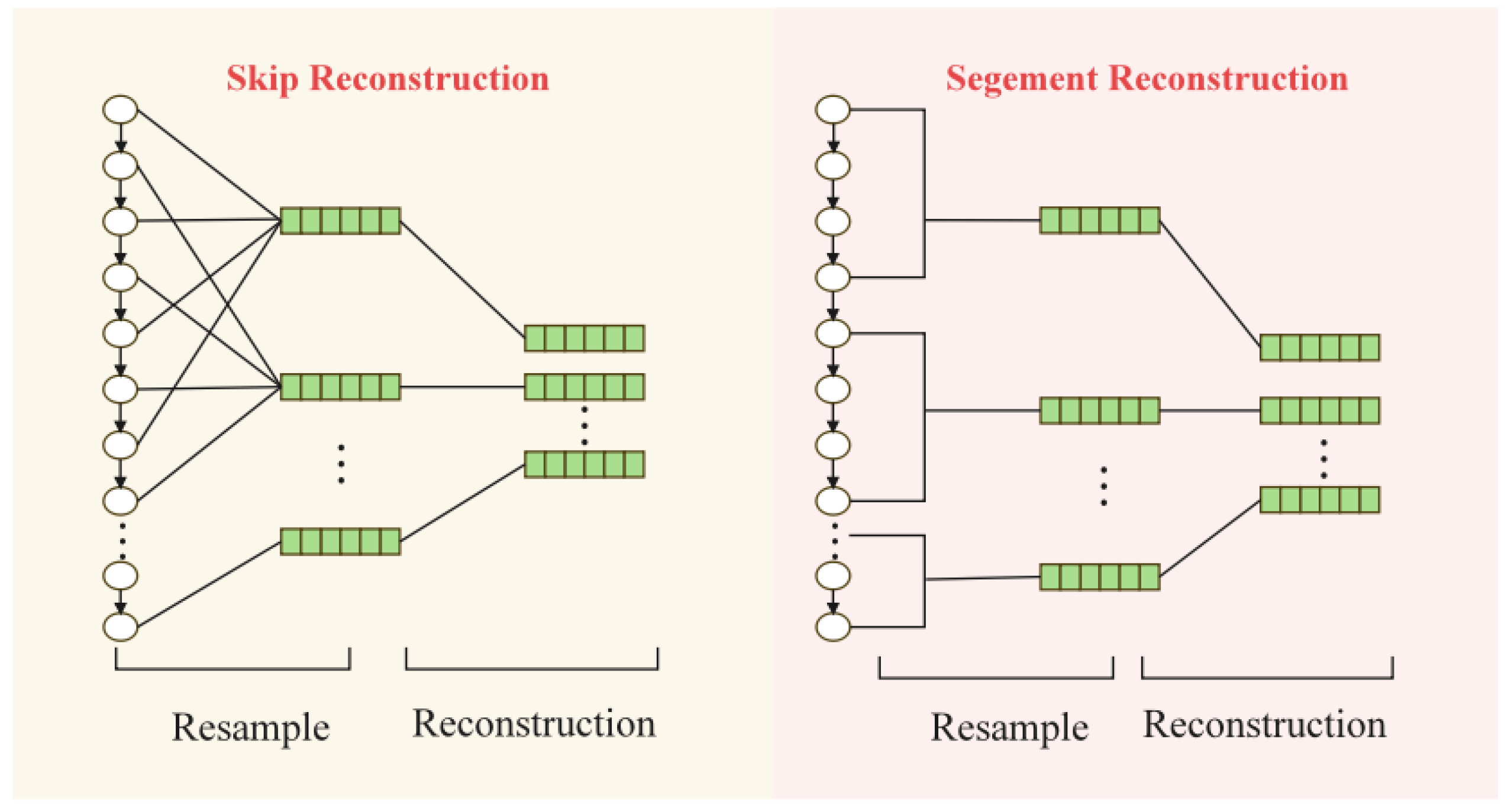
Before conducting time-localized attention calculations, the continuous one-dimensional load data needs to be reconstructed into a feature matrix, transforming it from a vector format into a matrix format. Given a historical load data sequence , with as the total number of historical load samples, the goal of feature reconstruction is to convert this sequence into a matrix with dimensions . As shown in Figure 1, there are two methods for feature reconstruction: the first method is to perform jump sampling on the original load sequence at intervals of , creating column vectors ; the second method segments the sequence at intervals of , with each segment forming column vectors . The matrices formed by these two methods are transposed versions of each other.
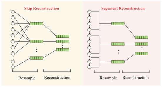
Figure 1.
Load feature reconstruction.
2.1.2. LSTM-Based Time Series Vector Learning
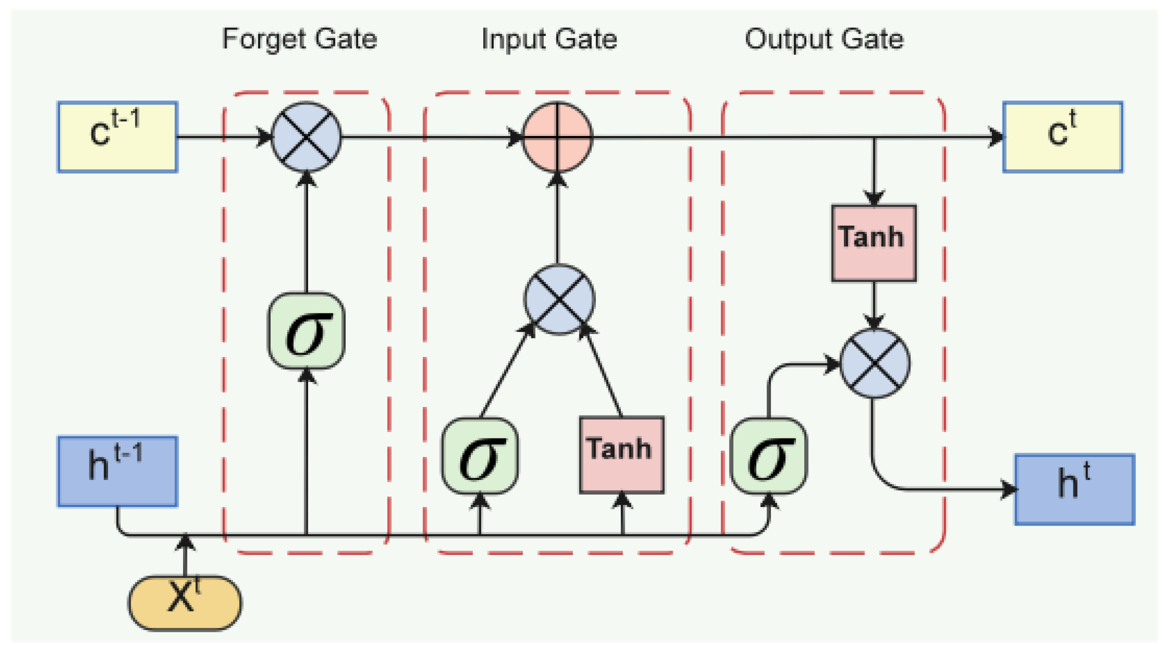
Compared to traditional RNNs with only one hidden state, LSTM introduces the concept of cell states, considering the temporal correlation hidden in long-term states. The cell structure of LSTM is shown in Figure 2.

Figure 2.
LSTM neuron structure.
Based on the recurrent neural network, LSTM adds input, forget, and output gates to control information flow input, output, and cell state, respectively, thereby managing the update of cell states. To calculate the output of an LSTM cell, calculations must be performed in the input gate, forget gate, and output gate, considering both the current input and the previous cell state. The LSTM neural cell computation formula at time is as follows:
where is the cell state of the memory cell at time ; denotes the cell state at the previous moment; denotes the candidate state of the input; is all the outputs of the LSTM unit at time ; , , , and are the matrices of the coefficients and the vectors of the biases, respectively; is the activation function Sigmoid; is the input at time ; , and , are the inputs at time t and the outputs of the input, forget and output gates at time t, respectively.
The LSTM neural network in the encoder has a multi-layer network structure, where each layer is composed of multiple neural cells. The calculation formula for the hidden state at time given input at time is as follows:
where is the LSTM network and is the output of the LSTM at the previous moment. The cyclic learning process of LSTM for the complete sequence from to is illustrated in Figure 3.
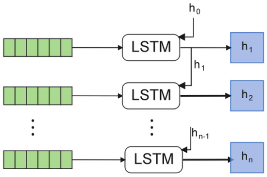
Figure 3.
LSTM learns time series vectors.
2.1.3. CNN-Based Time-Localized Convolution
The CNN, proposed by Lecun Y et al. in 1998, has been widely used in various deep learning fields such as image and speech processing [36]. The CNN extracts local features from data through local connections, weight sharing, and spatial pooling, demonstrating strong abstraction capabilities. As shown in Figure 4, its main structure includes convolutional, pooling, and fully connected layers [37]. The main formula for the CNN network is as follows:
where is the -th output of the -th convolutional layer, denotes the convolution operation, is the -th weight of the -th convolution kernel in the -th convolution layer, is the -th bias coefficient of the -th convolution layer, is the activation function, and is the activated output of the -th convolution in the -th layer.

Figure 4.
Convolutional network.
During local feature extraction, the CNN uses a convolution kernel of size to perform convolution operations on input . By adding padding as shown in Formula (3), the convolution output retains the same size as the original input matrix, resulting in an output with column vector form .
2.1.4. Attention Calculation
After obtaining the time sequence vector and time-localized features, attention scores are calculated for the time sequence vector based on the local features. This paper uses bilinear dot product to generate attention scores, and the calculation of attention scores for local features with respect to is as follows:
where is the linear transformation matrix, which scales the matrix multiplication.
This paper uses a soft attention method for local feature attention weighting. First, the attention weights for all local features are calculated. The attention weight calculation formula for local features is as follows:
where , and through weighting, the attention vector is obtained. Here, represents the fully connected network, with the calculation formula . In this formula, is the activation function, denotes the network parameters, is the input vector, and represents the bias term. Finally, the experiment compared three fusion methods: vector concatenation, element-wise product (Hadamard product), the matrix addition. The results indicated that the element-wise product performed the best. Therefore, this method was chosen to fuse the attention-weighted local vector with the time sequence vector , resulting in the time sequence output under local attention. The formula is as follows:
where represents the Hadamard product operation.
2.2. Temporal Local Attention LSTM Load Forecasting Network
The load forecasting network constructed in this paper divides the predicted output into three components: full-context regression output, date attention network output, and time-point attention network output. Each component value corresponds to a sub-neural network, and the overall structure is shown in Figure 5.
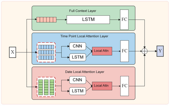
Figure 5.
Temporal Local Attention LSTM structure.
Full-context regression network: The full-context regression forecasting network comprises a conventional LSTM network. The LSTM processes data according to Formulas (1) and (2). Following the LSTM, a fully connected layer performs a linear transformation on the LSTM hidden layer to produce the output component .
Time-point local attention network: The time-point attention network is constructed based on the previously proposed temporal local attention mechanism. The purpose of this network is to identify the historical time-points that most significantly affect load forecasting. In the feature reconstruction step, jump sampling is used to construct the feature matrix. Using a daily interval as the sampling interval , and assuming that the load data are sampled at an hourly resolution, there will be 24 load values per day (i.e., ). The reconstructed feature matrix is input as column vectors into the LSTM sequentially, with the hidden state of the LSTM corresponding to the last input of used as the time series vector. Simultaneously, is input as a feature map into a CNN network, yielding the time-local convolution output . The time-point attention vector is calculated based on Formulas (4)–(6). After a final linear transformation through a fully connected layer, the time-point attention component is obtained.
Date local attention network: Similarly to the time-point local attention network, the date attention network is also built on the temporal local attention mechanism. The purpose of this network is to identify the historical dates with the most significant impact on predictive performance. Unlike the time-point local attention network, this network uses segmented sampling to construct the feature matrix during the feature reconstruction phase. Assuming an hourly sampling resolution, each segment size is , resulting in . The remaining steps are the same as in the time-point local attention network. The final output of the date local attention network is .
After computing the outputs from the three sub-networks, their components are combined to produce the final prediction output .
3. Case Studies
The experiments in this paper were conducted on a server running Ubuntu 16.04, equipped with an NVIDIA GTX 3090 GPU and an Intel i9-10100 CPU. All code was implemented primarily using Python 3.8, PyTorch 1.18, and Sci-Learn 1.11.
3.1. Dataset
The UMass Smart Dataset, 2017 release home dataset, contains electricity usage data for seven households from 2014 to 2016. It provides detailed records, at a 30 min frequency, of various household appliances’ power loads, including washing machines, air-conditioning units, and lighting systems. The model proposed in this paper uses hourly data from a week to predict the electricity load for the next hour. Therefore, the training employs a sliding window approach, with the window size being one week (i.e., 168 h) and the interval being one hour. Under extreme conditions, such as abnormal load data recorded by the meter leading to completely random data or prolonged periods of zero, the prediction performance may be affected, which is also unavoidable in other models.
To evaluate the performance of the model, this paper selected external datasets from 2014 to 2016 based on data quality and fluctuation (standard deviation). These datasets consist of half-hourly data. The data were first categorized by year (2014, 2015, 2016), and load anomalies (values equal to zero) were removed. The standard deviation of the data for each year was then calculated: 0.453 for 2014, 0.234 for 2015, and 0.224 for 2016. Consequently, the 2014 dataset, which exhibited greater variability, was selected. Furthermore, the fourth quarter of 2014, containing a higher concentration of anomalous data, was excluded, resulting in the final training and testing datasets. The dataset was split into training, validation, and test sets in an 8:1:1 ratio. Among them, the load of all electrical equipment and systems is summed, and the total household electricity load obtained is used as the prediction target, so there is no need for feature selection. In addition, max-min normalization was adopted for data preprocessing.
3.2. Error Evaluation Metrics
This paper uses MAE, MSE, RMSE, MAPE, and sMAPE to evaluate prediction errors, where smaller values indicate more accurate model predictions. Additionally, R2 is employed to measure the model’s ability to explain the variance in the target variable, with values closer to one indicating a better fit. The formulas are as follows:
where represents the number of load values, the actual load values, and the predicted values from the model.
3.3. Comparison of Models and Parameter Settings
Currently, traditional models such as LSTM and RNN remain among the best baseline models [38,39,40]. Therefore, this paper selects four traditional models—SVR, RFR, RNN, and LSTM—as comparison models.
3.3.1. Loss Function Configuration
The neural network is trained using a backpropagation algorithm. During training, the Adam Optimizer [41] with an MSE loss function is selected, with the MSE loss function defined as follows:
where represents all trainable parameters in the model.
3.3.2. Hyperparameter Configuration
The proposed model includes a total of four hyperparameters, with representing the number of LSTM layers, and the kernel size of the CNN network. All model hyperparameters are summarized in Table 1.

Table 1.
Hyperparameter configuration.
3.4. Prediction Performance
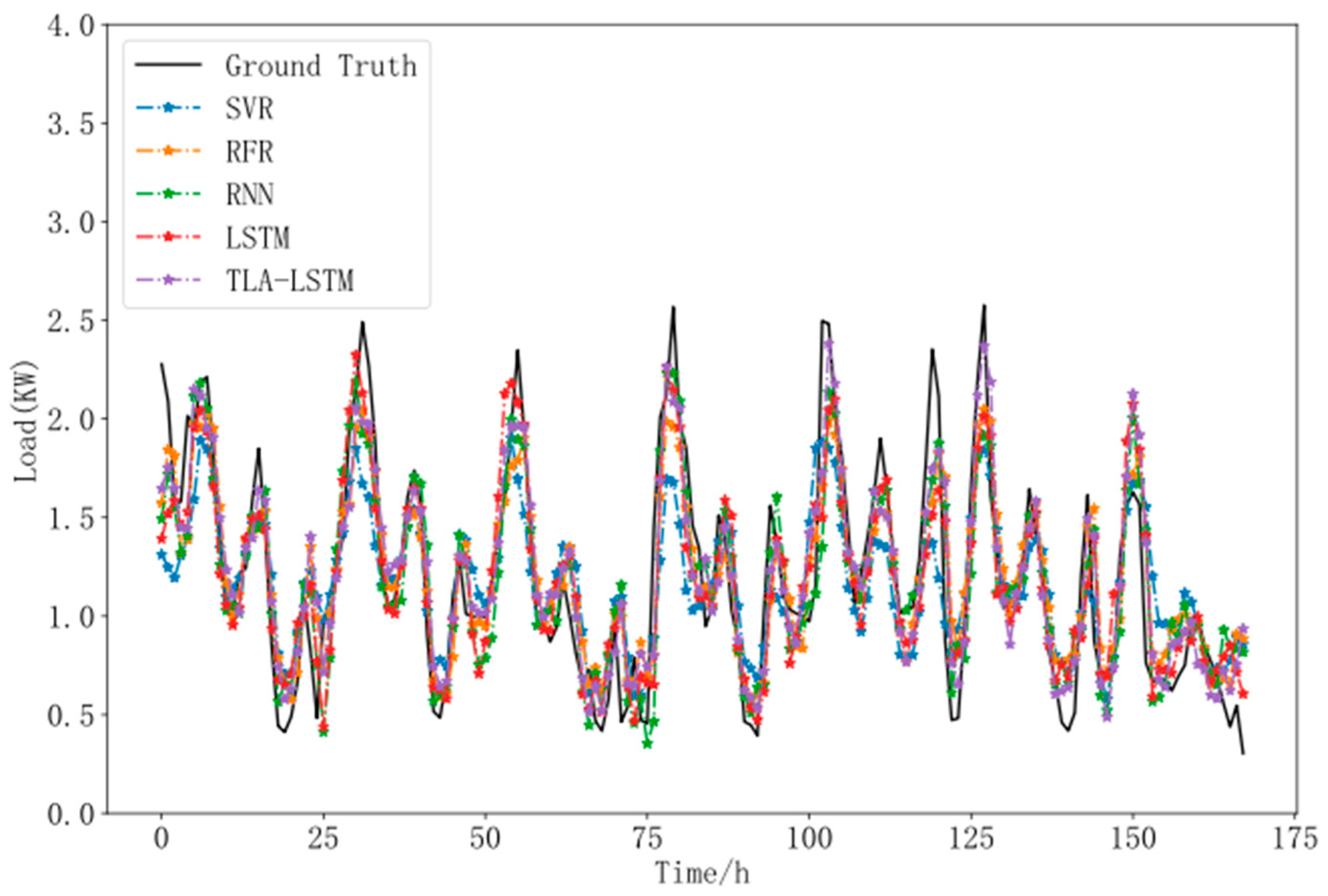
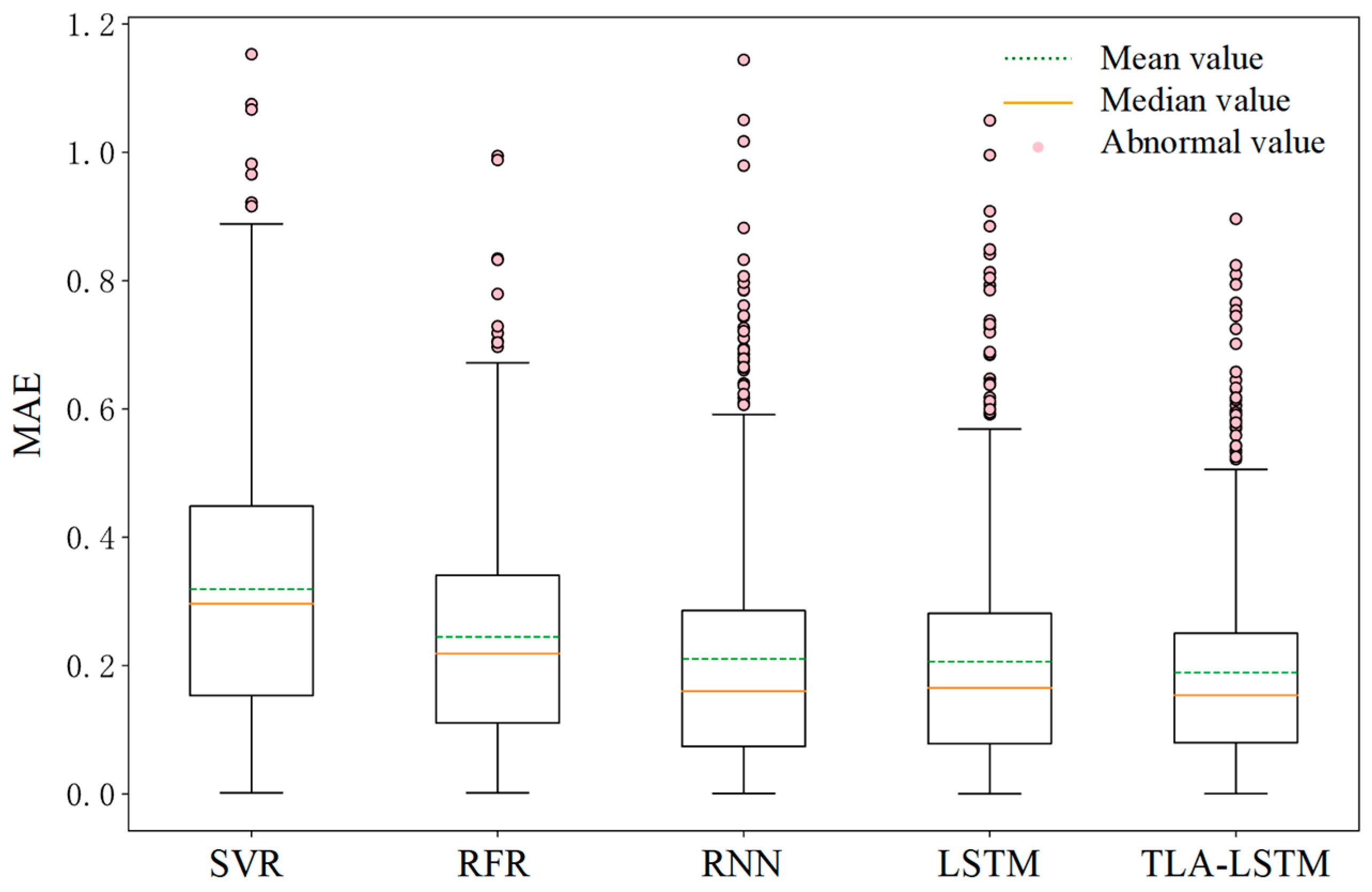
From Figure 6 and Table 2, it is evident that the traditional machine learning model, SVR, performs the worst across all error metrics. The RFR algorithm, utilizing ensemble learning by combining multiple weak classifiers, shows a significant improvement in predictive performance over the SVR model; however, its R2 error indicates that its accuracy still requires enhancement. The RNN deep learning model demonstrates better suitability for residential load forecasting than traditional machine learning models such as SVR and RFR. By leveraging the recurrent design of the neural units, the RNN effectively captures the sequential dependency of time series and closely fits the trend of the load curve. However, it still has room for improvement in accurately capturing peak values and rapidly fluctuating load curves. The LSTM model, with its incorporation of memory and forget gates, improves the time dependency perception over the original RNN, achieving better performance than the RNN in R2, MAE, MSE, RMSE, and sMAPE metrics. However, it shows slightly inferior performance to the RNN in the MAPE metric, possibly due to rapid peak changes in the load curve. Additionally, as household energy usage is generally low, some extreme values may amplify error in the MAPE metric. Conversely, MAE and MSE are less affected by extreme low values, making LSTM significantly better than the RNN in absolute error and R2 performance.
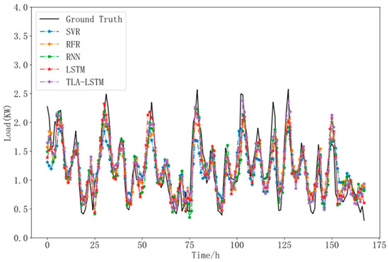
Figure 6.
Prediction results comparison.

Table 2.
Error statistics for all models.
Compared to the best-performing LSTM and RNN models, the TLA-LSTM model demonstrates notable enhancements across R2, MAE, MSE, RMSE, MAPE, and sMAPE metrics. Specifically, compared with the LSTM model, TLA-LSTM achieves a 14.2% improvement in R2, 8.2% in MAE, 15.2% in MSE, 8.5% in RMSE, and 6.4% in sMAPE, with a 3.8% improvement over the RNN in MAPE. By incorporating both date features and specific time-points into its temporal local attention mechanism, TLA-LSTM demonstrates strong robustness, delivering the most accurate predictions among all models tested.
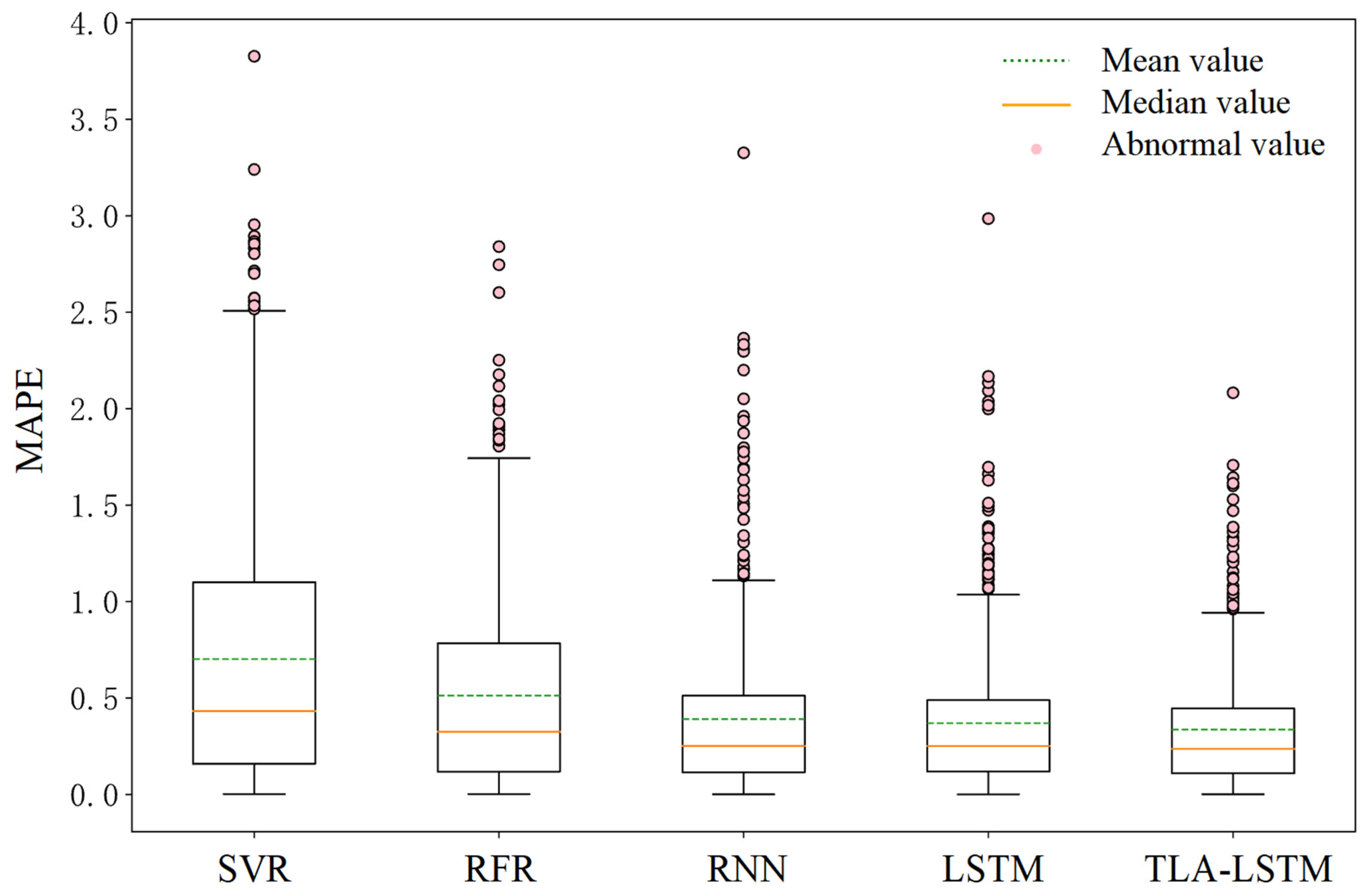
This paper compares the proposed TLA-LSTM model with SVR, RFR, RNN, and LSTM models in terms of predictive performance using box plots, with MAE and MAPE metrics employed to evaluate the stability of the results. As shown in Figure 7 and Figure 8, the proposed TLA-LSTM framework demonstrates superior error stability compared to the competing models. However, frequent outliers in the box plots can be attributed to the instability of load data and the scope for further improvement in predictive performance. From the prediction results, it can be observed that for certain regular load patterns, the proposed framework outperforms commonly used models in residential load forecasting in terms of accuracy.
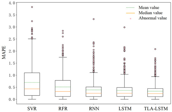
Figure 7.
Box plot of MAPE error.
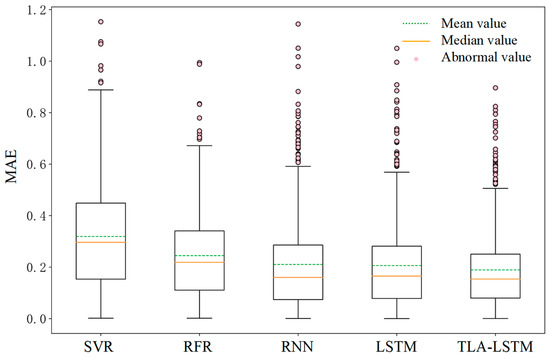
Figure 8.
Box plot of MAE error.
3.5. Window Size Experiment
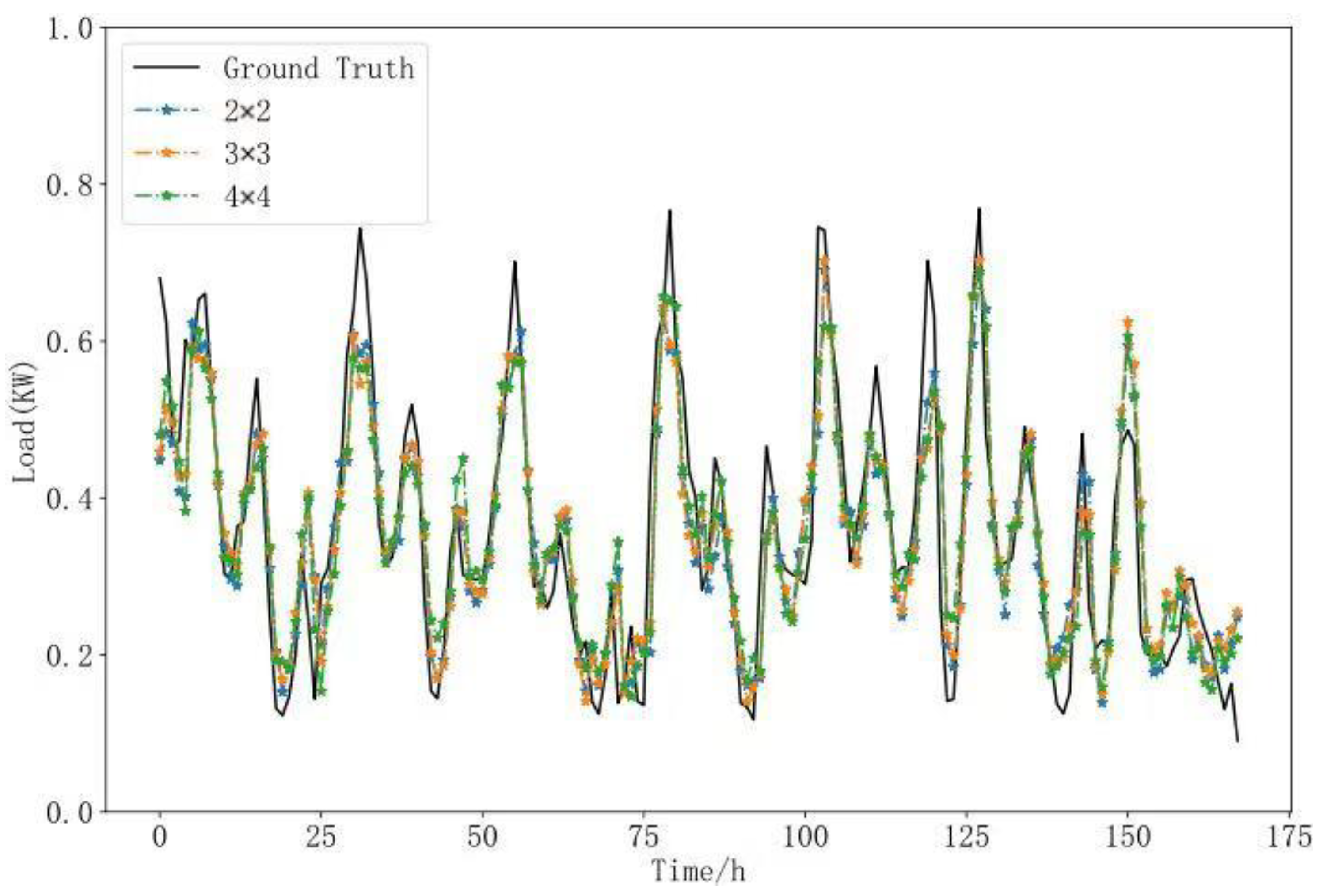
To further investigate the effect of the CNN convolutional window size in local time attention on network performance, the study validated prediction performance using convolution kernel sizes of 2 × 2 and 4 × 4 under identical experimental conditions. The prediction results are shown in Figure 9 below.
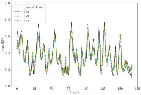
Figure 9.
Prediction results of window size experiment.
As shown in Table 3, compared with the 2 × 2 local convolution window size, the 3 × 3 window size has a larger receptive field, enhancing network performance. Although a 4 × 4 convolution window further expands the receptive field, it results in decreased performance compared to the 3 × 3 network due to noise information in the larger local window. Compared with the 2 × 2 window size, the 4 × 4 window demonstrates better performance in R2, with minimal differences in MAE, MSE, and MAPE. However, in the MAPE metric, the 4 × 4 window shows a noticeable decrease in performance, while it achieves better sMAPE, suggesting that a larger local window size may impact prediction performance for certain extreme values.

Table 3.
Error statistics for window size experiment.
4. Conclusions
This paper proposes a residential load forecasting model (TLA-LSTM) based on the TLA mechanism and LSTM network. By introducing the time-localized attention mechanism and combining CNN for local feature extraction from load data, the modeling capability of LSTM for time series data is further enhanced. Experimental results show that, compared to traditional models such as SVR, RFR, RNN, and standard LSTM, TLA-LSTM demonstrates significant improvements across multiple metrics.
In addition to the improvement in prediction accuracy, this research also provides positive support for achieving sustainability goals. As smart grids and distributed energy systems continue to develop, accurate residential load forecasting can effectively help power companies optimize pricing structures, reduce energy waste, and enhance energy efficiency. Furthermore, the TLA-LSTM model is better at sensing and adapting to the volatility and complexity of household loads, supporting personalized demand response strategies, and contributing to the goals of a low-carbon economy and green power systems.
Although the experimental results on offline data demonstrate the model’s effectiveness, future research could further enhance the model’s real-time learning capabilities to address dynamically changing load demands. Moreover, with the inclusion of more exogenous variables, the model’s predictive power is expected to improve further. In the future, by integrating continuous learning mechanisms and optimizing with real-time data, the TLA-LSTM model can be applied to develop demand-corresponding strategies to contribute to peak-and-valley reduction in electricity loads.
Author Contributions
Conceptualization, W.C. and Y.Z.; methodology, W.C. and H.L.; software, H.L. and X.Z.; validation, X.Z. and Y.Z.; formal analysis, W.C. and H.L.; investigation, Y.Z. and X.Z.; data curation, W.C. and H.L.; writing—original draft, W.C. and H.L.; writing—review and editing, W.C., Y.Z. and H.L.; visualization, W.C. and H.L.; supervision W.C. and Y.Z.; project administration, Y.Z.; funding acquisition, W.C. All authors have read and agreed to the published version of the manuscript.
Funding
This work was supported in part by the National Natural Science Foundation of China (Grant no. 72274058), the Hunan Province Education Department General Project for Teaching Reform in Colleges and Universities (Grant no. HNJG-20230794), the Major Project of Xiangjiang Laboratory in China (Grant no. 23XJ01008), and the Interdisciplinary Research Project at Hunan University of Technology and Business, China (Grant no. 2023SZJ01).
Institutional Review Board Statement
Not applicable.
Informed Consent Statement
Not applicable.
Data Availability Statement
The data presented in this study are available on request from the first author.
Conflicts of Interest
The authors declare no conflicts of interest.
References
- Imani, M.; Ghassemian, H. Residential load forecasting using wavelet and collaborative representation transforms. Appl. Energy 2019, 253, 113505. [Google Scholar] [CrossRef]
- Danish, M.S.S.; Sabory, N.R.; Ahmadi, M.; Senjyu, T.; Majidi, H.; Abdullah, M.A.; Momand, F. Energy and Environment Efficiencies Towards Contributing to Global Sustainability. In Sustainability Outreach in Developing Countries; Springer: Singapore, 2020; pp. 1–13. [Google Scholar] [CrossRef]
- Yildiz, B.; Bilbao, J.; Dore, J.; Sproul, A. Recent advances in the analysis of residential electricity consumption and applications of smart meter data. Appl. Energy 2017, 208, 402–427. [Google Scholar] [CrossRef]
- Yang, Y.; Li, W.; Gulliver, T.; Li, S. Bayesian Deep Learning-Based Probabilistic Load Forecasting in Smart Grids. IEEE Trans. Ind. Inform. 2020, 16, 4703–4713. [Google Scholar] [CrossRef]
- Zhang, L.; Zhang, B. Scenario Forecasting of Residential Load Profiles. IEEE J. Sel. Areas Commun. 2020, 38, 84–95. [Google Scholar] [CrossRef]
- Haben, S.; Arora, S.; Giasemidis, G.; Voss, M.; Vukadinović, G. Review of low voltage load forecasting: Methods, applications, and recommendations. Appl. Energy 2021, 304, 117798. [Google Scholar] [CrossRef]
- Li, Y.; Han, D.; Yan, Z. Long-term system load forecasting based on data-driven linear clustering method. J. Mod. Power Syst. Clean Energy 2018, 6, 306–316. [Google Scholar] [CrossRef]
- Lee, C.; Ko, C. Short-term load forecasting using lifting scheme and ARIMA models. Expert Syst. Appl. 2011, 38, 5902–5911. [Google Scholar] [CrossRef]
- Haben, S.; Giasemidis, G.; Ziel, F.; Arora, S. Short term load forecasting and the effect of temperature at the low voltage level. Int. J. Forecast. 2019, 35, 1469–1484. [Google Scholar] [CrossRef]
- Litjens, G.; Worrell, E.; van Sark, W. Assessment of forecasting methods on performance of photovoltaic-battery systems. Appl. Energy 2018, 221, 358–373. [Google Scholar] [CrossRef]
- Danish, M.S.S. A Framework for Modeling and Optimization of Data-Driven Energy Systems Using Machine Learning. IEEE Trans. Artif. Intell. 2023, 5, 2434–2443. [Google Scholar] [CrossRef]
- Chen, Y.; Xu, P.; Chu, Y.; Li, W.; Wu, Y.; Ni, L.; Bao, Y.; Wang, K. Short-term electrical load forecasting using the Support Vector Regression (SVR) model to calculate the demand response baseline for office buildings. Appl. Energy 2017, 195, 659–670. [Google Scholar] [CrossRef]
- Chen, B.; Chang, M.; Lin, C. Load Forecasting Using Support Vector Machines: A Study on EUNITE Competition 2001. IEEE Trans. Power Syst. A Publ. Power Eng. Soc. 2004, 19, 1821–1830. [Google Scholar] [CrossRef]
- Xu, L.; Wang, S.; Tang, R. Probabilistic load forecasting for buildings considering weather forecasting uncertainty and uncertain peak load. Appl. Energy 2019, 237, 180–195. [Google Scholar] [CrossRef]
- Raza, M.; Nadarajah, M.; Hung, D.; Baharudin, Z. An intelligent hybrid short-term load forecasting model for smart power grids. Sustain. Cities Soc. 2017, 31, 264–275. [Google Scholar] [CrossRef]
- Danish, M.S.S.; Ahmadi, M.; Ibrahimi, A.M.; Dinçer, H.; Shirmohammadi, Z.; Khosravy, M.; Senjyu, T. Data-Driven Pathways to Sustainable Energy Solutions; Springer Nature: Cham, Switzerland, 2024; pp. 1–31. [Google Scholar] [CrossRef]
- Khodayar, M.; Kaynak, O.; Khodayar, M. Rough Deep Neural Architecture for Short-Term Wind Speed Forecasting. IEEE Trans. Ind. Inform. 2017, 13, 2770–2779. [Google Scholar] [CrossRef]
- Dedinec, A.; Filiposka, S.; Dedinec, A.; Kocarev, L. Deep belief network based electricity load forecasting: An analysis of Macedonian case. Energy 2016, 115, 1688–1700. [Google Scholar] [CrossRef]
- Kuo, P.; Huang, C. A High Precision Artificial Neural Networks Model for Short-Term Energy Load Forecasting. Energies 2018, 11, 213. [Google Scholar] [CrossRef]
- Afrasiabi, M.; Mohammadi, M.; Rastegar, M.; Kargarian, A. Probabilistic deep neural network price forecasting based on residential load and wind speed predictions. IET Renew. Power Gener. 2019, 13, 1840–1848. [Google Scholar] [CrossRef]
- Rahman, A.; Srikumar, V.; Smith, A. Predicting electricity consumption for commercial and residential buildings using deep recurrent neural networks. Appl. Energy 2018, 212, 372–385. [Google Scholar] [CrossRef]
- Qin, J.; Zhang, Y.; Fan, S.; Hu, X.; Huang, Y.; Lu, Z.; Liu, Y. Multi-task short-term reactive and active load forecasting method based on attention-LSTM model. Int. J. Electr. Power Energy Syst. 2022, 135, 107517. [Google Scholar] [CrossRef]
- Kong, W.; Dong, Z.; Jia, Y.; Hill, D.; Xu, Y.; Zhang, Y. Short-Term Residential Load Forecasting Based on LSTM Recurrent Neural Network. IEEE Trans. Smart Grid 2019, 10, 841–851. [Google Scholar] [CrossRef]
- Cheng, X.; Wang, L.; Zhang, P.; Wang, X.; Yan, Q. Short-term fast forecasting based on family behavior pattern recognition for small-scale users load. Clust. Comput. 2022, 25, 2107–2123. [Google Scholar] [CrossRef]
- Luong, M.; Pham, H.; Manning, C. Effective Approaches to Attention-based Neural Machine Translation. arXiv 2015. [Google Scholar] [CrossRef]
- Li, L.; Tang, S.; Zhang, Y.; Deng, L.; Tian, Q. GLA: Global–Local Attention for Image Description. IEEE Trans. Multimed. 2018, 20, 726–737. [Google Scholar] [CrossRef]
- Cinar, Y.G.; Mirisaee, H.; Goswami, P.; Gaussier, E.; Aït-Bachir, A. Period-aware content attention RNNs for time series forecasting with missing values. Neurocomputing 2018, 312, 177–186. [Google Scholar] [CrossRef]
- Alhussein, M.; Aurangzeb, K.; Haider, S. Hybrid CNN-LSTM Model for Short-Term Individual Household Load Forecasting. IEEE Access 2020, 8, 180544–180557. [Google Scholar] [CrossRef]
- Kim, T.; Cho, S. Predicting residential energy consumption using CNN-LSTM neural networks. Energy 2019, 182, 72–81. [Google Scholar] [CrossRef]
- Zang, H.; Xu, R.; Cheng, L.; Ding, T.; Liu, L.; Wei, Z.; Sun, G. Residential load forecasting based on LSTM fusing self-attention mechanism with pooling. Energy 2021, 229, 120682. [Google Scholar] [CrossRef]
- Wang, S.; Wang, X.; Wang, S.; Wang, D. Bi-directional long short-term memory method based on attention mechanism and rolling update for short-term load forecasting. Int. J. Electr. Power Energy Syst. 2019, 109, 470–479. [Google Scholar] [CrossRef]
- Li, C.; Dong, Z.; Ding, L.; Petersen, H.; Qiu, Z.; Chen, G. Interpretable Memristive LSTM Network Design for Probabilistic Residential Load Forecasting. IEEE Trans. Circuits Syst. I Regul. Pap. 2022, 69, 2297–2310. [Google Scholar] [CrossRef]
- Lin, J.; Ma, J.; Zhu, J.; Cui, Y. Short-term load forecasting based on LSTM networks considering attention mechanism. Int. J. Electr. Power Energy Syst. 2022, 137, 107818. [Google Scholar] [CrossRef]
- Yousaf, S.; Bradshaw, C.R.; Kamalapurkar, R.; San, O. Investigating critical model input features for unitary air conditioning equipment. Energy Build. 2023, 284, 112823. [Google Scholar] [CrossRef]
- Aseeri, A. Effective RNN-Based Forecasting Methodology Design for Improving Short-Term Power Load Forecasts: Application to Large-Scale Power-Grid Time Series. J. Comput. Sci. 2023, 68, 101984. [Google Scholar] [CrossRef]
- Lecun, Y.; Bottou, L.; Bengio, Y.; Haffner, P. Gradient-based learning applied to document recognition. Proc. IEEE 1998, 86, 2278–2324. [Google Scholar] [CrossRef]
- Chen, K.; Chen, F.; Lai, B.; Jin, Z.; Liu, Y.; Li, K. Dynamic Spatio-Temporal Graph-Based CNNs for Traffic Flow Prediction. IEEE Access 2020, 8, 185136–185145. [Google Scholar] [CrossRef]
- Singh, G.; Bedi, J. A federated and transfer learning based approach for households load forecasting. Knowl.-Based Syst. 2024, 299, 111967. [Google Scholar] [CrossRef]
- Lin, W.; Wu, D.; Jenkin, M. Electric Load Forecasting for Individual Households via Spatial-temporal Knowledge Distillation. IEEE Trans. Power Syst. 2024, 1–13. [Google Scholar] [CrossRef]
- Mubarak, H.; Stegen, S.; Bai, F.; Abdellatif, A.; Sanjari, M. Enhancing interpretability in power management: A time-encoded household energy forecasting using hybrid deep learning model. Energy Convers. Manag. 2024, 315, 118795. [Google Scholar] [CrossRef]
- Kingma, D.; Ba, J. Adam: A Method for Stochastic Optimization. arXiv 2017. [Google Scholar] [CrossRef]
Disclaimer/Publisher’s Note: The statements, opinions and data contained in all publications are solely those of the individual author(s) and contributor(s) and not of MDPI and/or the editor(s). MDPI and/or the editor(s) disclaim responsibility for any injury to people or property resulting from any ideas, methods, instructions or products referred to in the content. |
© 2024 by the authors. Licensee MDPI, Basel, Switzerland. This article is an open access article distributed under the terms and conditions of the Creative Commons Attribution (CC BY) license (https://creativecommons.org/licenses/by/4.0/).

