Optimizing Energy Consumption of Industrial Robots with Model-Based Layout Design

Abstract

The paper describes the development of an optimization model for the layout of an industrial robot relative to known locations of served machines and operations to be performed. Robotized material handling applications, defined by trajectories (paths, speed profiles) and final points, are considered in this research. An energy-monitoring framework set up by joint velocities provides input data that are fed to the optimization model. The physical placement of the robot base stands for the decisional variables, while the objective function is represented by the total distance covered by individual joints along established task routes transposed into energy consumption. The values of the decisional variables are restricted by trajectory constraints (waypoints on paths), joint operating values and link dimensions. Modelling technique and practical results using the Microsoft Solver optimization tool from Excel for Microsoft 365, Version 2312 are reported for SCARA-type robots. The performance of the optimization model is compared with actual measurements of consumed energy on an Adept Cobra S600 SCARA robot.

1. Introduction

The number of machines with digital control equipment used in industrial processes is constantly increasing [1,2,3], allowing high levels of precision, speed, and determinism to be achieved. At the same time, the recent period is characterized by large increases in energy costs, which led to a general pressure to reduce energy consumption (EC) in industrial processes [4,5]. Energy efficiency of equipment has become an increasingly important feature of industrial applications [6,7,8,9].

As a result, the process of ensuring energy efficiency must start from the application design and solution implementing stage and continue with the detailed analysis of the current functioning and the identification of equipment that can be upgraded or whose operation can be optimized by adjusting parameters or by globally reconfiguring tasks.

The automation of distributed industrial processes has led to the consolidation of IP/Ethernet networks in factories, creating new opportunities for connecting equipment aimed at increasing the awareness of EC. The appearance of Wi-Fi devices (802.11) in industrial environments and implicitly the development of networks of this type further supports the growth of the Internet of Things (IoT) segment due to the ease of implementing such solutions [10,11].

An analysis of the most efficient strategies that optimize EC of industrial robots is presented in [12]. Thus, optimizing path planning and trajectory generation involves efficient programming to limit unnecessary robot movements and changes in directions of joint displacements [13], reduce overall travel distances and tune parameters of the speed profile (cruise speed, acceleration, deceleration), select the best energy-saving robot configuration (e.g., righty/lefty) for the assigned motions [14], apply minimum jerk trajectory control [15], and generally use the continuous-path motion feature [16].

EC can be significantly reduced by including energy-saving features in the robot operating mode. Power management systems can be programmed to switch the robot to a low-power state when it is idle, in standby, or at the occurrence of some types of events; in such cases, power is temporarily disabled for some components or shut off for the entire robot manipulator [17]. Reducing idle times of industrial robots waiting for material components (e.g., parts travelling on conveyor belts), acknowledge signals from partner equipment (e.g., Programmable Logic Controller (PLCs), storage controllers), and confirmations from human operators implies a proper synchronization of robot tasks with inventory, transport, and processing material flows to reduce EC [18].

Regenerative braking can be used to recuperate the energy that is normally lost during braking time of industrial robots working schedules [19]. In applications like part handling, product palletizing and assembling, industrial robots perform many downward or lateral movements during which the actuators dissipate energy, thereby potentially generating electricity. Intelligent braking management systems and the temporal storage of energy in a capacitive buffer have been proposed to recover energy. The work [20] presents two approaches for saving the recuperated energy: a capacitive energy buffer on the robot’s DC-bus and the robot EnergyTeam principle. The latter consists in the DC-bus of industrial robot power controllers enabling a controlled energy flow in a resource team (robot cluster) among the robots that currently decelerate and therefore recuperate the energy, and those that require simultaneously a peak power supply to accelerate. These methods imply, however, important adaptations in robot hardware, which involve high initial investment costs and therefore limit their frequent adoption. In older robot systems on the market, the resulting energy is converted to waste heat by control technology through electrical resistance and dissipated into the environment. With the rapid progress of electric vehicles in recent years, the systematization and application of knowledge in one of the areas of electric vehicle control, i.e., energy management issues when using braking controllers, has also addressed robotics [21,22].

At present, Yaskawa offers a technical solution for the recovery of robot braking energy into the power grid—as a standard and without additional hardware and can be thus reused. All larger Motoman robot series with a payload upwards of approximately 50 kg and the latest YRC1000 robot controls can convert kinetic energy from down and sideways movements directly into 400 V AC at 50 Hz and feed it back into the net [23]; depending on its movement pattern, the robot’s energy requirements are thereby significantly reduced.

More recent data-driven optimization strategies exploit big data streaming, data analytics, machine learning, and artificial intelligence techniques to optimize EC of industrial robots. The analysis of historical time series and large amounts of real-time data is used to identify EC patterns and predict consumptions for robot operations at production batch horizon, assign operation types to robots in energy-aware mode, adjust motion parameters, and provide operative insights for energy-saving and optimization strategies. These strategies mainly provide support for energy-efficient trajectory planning and predict EC to weight the participation of robots in production tasks.

Data-driven optimized motion planning is approached in [24], where a set of predefined motion trajectories are followed by an industrial robot while the EC is measured. The data sets obtained by associating trajectory data with measured energy data are then used to train a machine learning model which provides a fitness function to evolution based or swarm-intelligence algorithms to obtain a near-optimal EC robot trajectory. In the study [25], the authors apply metaheuristic theories (genetic algorithm and particle swarm optimization) to obtain energy efficiency in different dual-arm robot configurations for part retrieval and placing on a conveyor belt. Neural network methods are used in [26] to identify non-linear dependencies in EC models for industrial robots that perform processes characterized by complex trajectories: palletizing packages, loading/unloading of machines, and contact welding. These models are then used to adjust motion parameters (speed, acceleration) to minimize EC.

Predicting EC of industrial robots integrated in intelligent manufacturing systems offers premises for efficiency. A methodology for the reliable prediction of EC of robots serving in manufacturing processes is given in [27]; the established EC models help to allocate energy cost to products, to calculate the product carbon footprint, and to define and validate measures to improve energy efficiency in production. The research reported in [28] describes a data-driven modelling approach using a batch-normalized long short-term memory (BN-LSTM) network to construct a robust energy-consumption prediction model for industrial robots before they are used in production systems.

Global optimization of the energy consumed by robot teams in batch production using machine learning (ML) techniques is applied in large-scale manufacturing systems. In [29], an architecture is proposed that uses big data concepts and map-reduce algorithms to process the information streams in multiple-robot manufacturing systems, focusing on EC aggregated at various layers. Once the EC information is aggregated in logical streams and consolidated based on relevant meta-data, a neural network is trained and used to determine possible faults or variations from the normal patterns of EC at each layer. This novel approach allows accurate forecasting of EC patterns in real time in the production cycle, by using long short-term memory (LSTM) neural networks and real-time classifiers in two stages:

• For energy-aware batch planning—over the long term: real-time optimization of operations scheduling/products and their allocation/robot for the entire batch of products to be executed based on the prediction of EC of robots for each type of operation; the minimization of the total energy consumed by all active robots is considered.
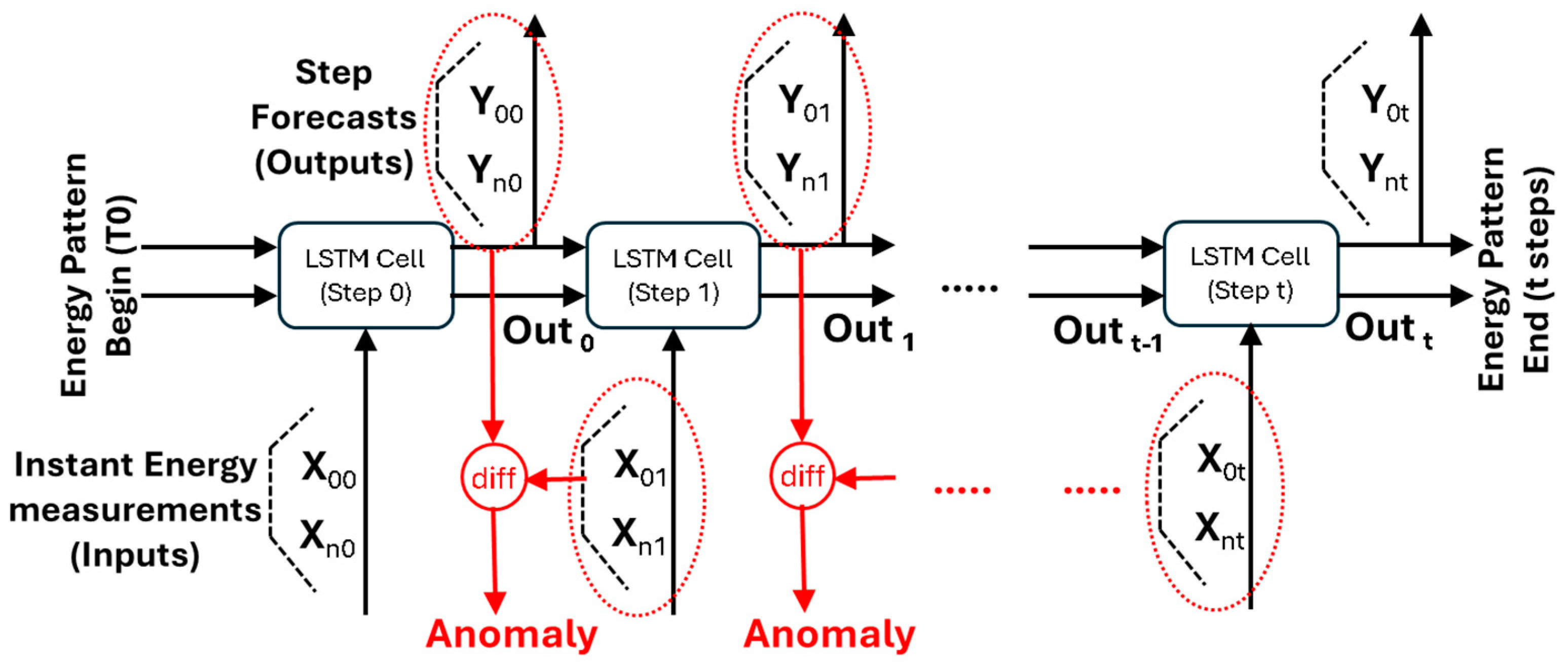
• For robot health monitoring—in the short term: whenever an anomaly or a significant increase in the energy consumed by a robot is detected, the resource is isolated and its maintenance program is launched.

The LTSM module is used for the prediction of instant EC of robots to provide a more accurate input for the cloud-based System Scheduler, i.e., the optimization module that performs mixed product and operation scheduling plus allocation on resources (robots): instead of the last recorded EC values, forecasted values at batch execution horizon are used as input for optimization (Figure 1). The parameters that are used as input data for the optimization engine are the operation execution time and the EC per operation of each robot. In this architecture, the ML-based prediction module and the centralized optimization module work in parallel, being interconnected by a multi-dimensional energy data buffer which is:

• Updated by the prediction module each time the complete execution of an operation is recorded, and
• Read by the optimization module each time a new production schedule needs to be computed.

Most of the developed EC optimization strategies impose monitoring the energy consumed by robots during their working period, which assumes (a) continuously measuring EC and computing the consumption values accumulated during significant periods: operation completion, product construction, batch execution; (b) identifying patterns of EC for motion types, segments, and sequences at the operation level; (c) setting up EC models and comparing their data with EC data collected in real time to detect deviations and generate ad hoc decisions for robot health protection; (d) combining energy measurements with historical data to globally optimize production tasks performed with multiple industrial robots.

From the analysis of the available literature, a set of measures taken in the design phase of industrial processes and infrastructures have been identified to reduce at run time the EC of industrial robots integrated in production [3,30,31]. Among these, proper robot selection for specific operations reduces EC during working periods, and equipping robots with energy-efficient components such as actuators, transmission elements, batteries, and sensors additionally will reduce EC in real time. The design solutions reported in these papers consider: mechanical design, e.g., proper manipulator construction using light materials for links and motors; mathematical approaches, e.g., computation of energy-efficient motion paths with parameterized speed profiles; simulation approaches with model-driven digital twins [32] to relate motion to EC; and data-driven approaches that use smart meters to evaluate the electrical power flow from the supply network to the robot components, thus modelling the overall EC of the robot.

One common finding from these papers that report solutions minimizing by design the energy consumed by robots is the necessity to continuously observe robot operations and identify the factors that influence EC: imposed parameters of the speed profile and trajectory smoothness. This approach is preferable to mathematical modelling since it limits complexity and does not use motor load profiles (angular velocity, torque, elasticity, friction) which are only accessible to the manufacturers of industrial robots [6].

A novel method that can be applied off-line in the workstation design phase minimizes the overall EC of industrial robots during their entire lifecycle; this method, proposed in the current paper, computes the most energy-efficient positioning of the robot relative to a predetermined layout of the shop floor resources, e.g., computer numerically controlled (CNC) machines, conveyor belt, storage units, with which it interacts. The novelty of the approach consists in designing an energy-efficient shop floor layout that integrates the placement of industrial robots, selected according to reachability and payload requirements, relative to pre-established resource placements (e.g., machines) to be served in pre-assigned tasks.

The optimization solution presented in the article is designed to be applied to standard types of open kinematic (serial) industrial robots executing joint movements. Linear or linked movements (as in the case of Delta-type robots) are not considered. The idea is to separate a material-handling trajectory between fixed points into individual joint movements and compute the EC based on the distances covered by each joint.

The remainder of the manuscript is organized as follows: Section 2 associates the characteristics of an industrial robot which influence its EC to the optimization model from a systemic point of view (I/O approach) and describes the customized EC measurement solution which will provide the input to the optimization model. Section 3 presents the optimization problem for the placement of the robot executing closed trajectories, e.g., pick-and-place motion sequences. Section 4 presents how the input data are created from physical measurements and robot dimensions. Section 5 presents a case study which is validated against real consumption measured from the physical system. The last section consists of conclusions and future research directions.

2. Energy Consumption and Formation of the Optimization Model

2.1. Overview of Factors Affecting Energy Consumption by Industrial Robots

An industrial robot is an autonomous system comprising a physical manipulator driven by a computer-based controller that runs a program to perform specific operations in a manufacturing or processing line. The movement of the manipulator along with other controlled tasks contribute to the total EC [33,34,35] which is influenced by:

(a)

Types of industrial robots (anthropomorphic, SCARA, Delta, Cartesian, etc.): The design of articulated arms allows the mechanical structure to perform complex tasks, and demands significant power to move and maintain stability, especially when handling heavy payloads or moving at high speeds. The continuous need to counteract gravity, particularly when operating along the Z axis to lift objects, further increases the EC. Unlike simpler robots (e.g., SCARA, Cartesian, and other task-specific structures) which have limited planes of movement, e.g., serving primarily in a horizontally plane, vertical articulated robots work more frequently against gravitational forces.

(b)

Physical factors such as weight and inertia (distribution of weight) of segments: to provide repeatability and rigidity, robot segments are manufactured of heavier materials which influence the motors’ dimensions and hence their EC. This category also includes the end-effector design and payload limitations.

(c)

Robot programming through path specification (minimize motion commands, create smooth trajectories with fewer stop points) and motion control (adjust speed, acceleration, and deceleration according to process specifications) reduces EC either directly, by limiting motor consumption or indirectly, through cycle time reduction. This is the case in applications where the end-effector and its active time impacts the total EC of the workstation (e.g., laser cutting, welding) [36,37].

(d)

Control components such as sensors, joint controllers, and end-effector actuators influence the overall EC of the robot system. This EC is directly proportional to the operating time as in the case of robots with welding equipment.

(e)

Environmental factors such as ambient temperature, moving constraints, trajectory points (linked motions consume more energy than non-linked ones [38]), trajectory precision (using final points which force the robot to stop at designed points is more energy intensive than using fly-by points which are used to bring the tool control point in a certain point vicinity, not reducing the robot speed to zero [12]).

(f)

Alternation between stand-by mode, which uses mechanic brakes and working state, where electric breaks are activated, greatly influences EC in industrial applications where equipment is enabled only during production time.

A typical process employing an industrial robot for material handling is depicted in Figure 2, where the robot moves parts between a local storage (pick position) and a conveyor (place position) while passing through a safe position. When such a process is automated, the points of interest are fixed and there is flexibility when mounting the base of the robot [12]. Considering the elements presented above, it is possible to design a robotized workstation with the objective of minimizing EC. While techniques such as variable cruise speed and acceleration [12] or dynamic trajectory generation [13,24] have been studied, robot placement relative to the workplace has not been studied yet, to the best of our knowledge, considering the reported references.

In this respect, we propose a solution (Figure 2) that forms an EC model offline which is used as input for an optimization algorithm to compute the robot’s placement that will minimize EC at task execution. Input data fall into three categories: (a) data available from the robot manufacturer (robot type and link dimensions), (b) data available from the process (placement of points of interest on the route and obstacles to avoid), and (c) data that need to be created and represent the consumption of each joint drive for a unit of movement at different speed limitations.

These speed limitations must be considered because a simple movement between two points of interest is done with a speed profile obtained by scaling the velocity of each joint according to the ‘leading axis’ principle that ensures that all joint motions start and end at the same time. This process is depicted in Figure 3 and emphasizes the need for a robot EC model that will be created using the custom-made solution described in Section 3.

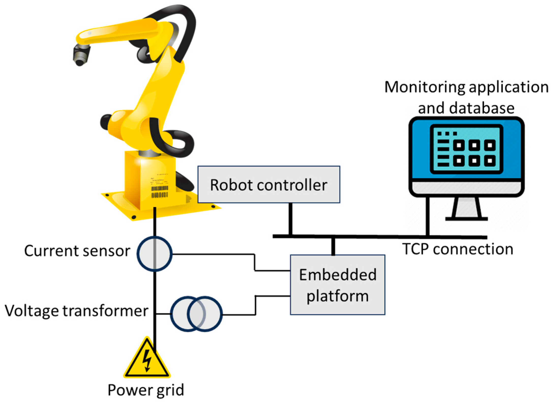
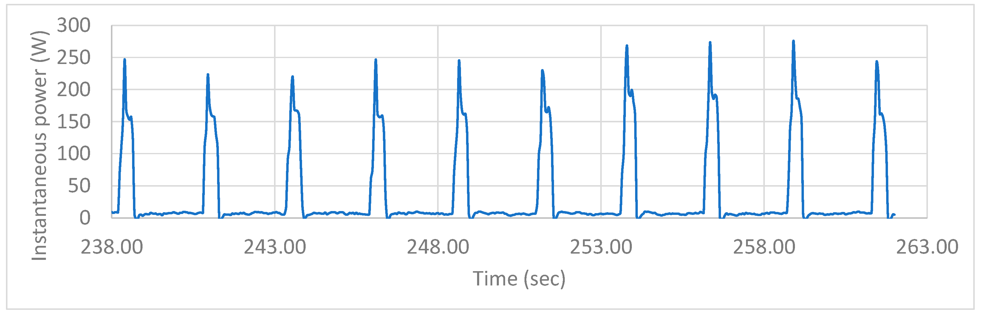
2.2. Measurement and Monitoring Technique

Commercial smart meters [38,39] are used in applications such as automated billing to compute the total EC over longer periods of time, and have fixed communication protocols [32,40]. They can generate power profile charts, but the resolution is not compatible with the needs of industrial robots which have small cycle times with fine power profiles that significantly influence the total EC of the application. To capture the particularities of robot trajectories, a special smart meter has been developed with the scope of generating the offline EC model used to establish the optimal robot placement with respect to known tasks and resource serving points that will minimize EC at run time.

The smart meter consists of a current clamp and a voltage transformer connected to an Intelligent Embedded Device (IED) capable of: (a) processing high volumes of data in real-time for filtering inputs, integrating voltage and current signals, and adjusting the phase shifts introduced by the measuring transformers, (b) communicating over the TCP/IP network in order to form the digital EC model and synchronize with the monitored process (robot motion operations), and (c) parallel processing in order to separate the instantaneous power integration from the synchronization and communication processes. Figure 4 shows a schematic representation of the connected smart meter.

Different commercial IED models have been studied, as shown in

Table 1. Commercial IED models.

Device	Characteristics
$\mathrm{Arduino} (\mathrm{with} \mathrm{Atmel} \mathrm{AVR} 8-\mathrm{bit} \mu$controller, 8 × 10-bit ADC)	Needs an external Wi-Fi interface. Reduced computing resources which are insufficient for network communication, data processing, and further software extensions/improvements.
ESP8266 (1 Tensilica 32-bit L106 core, 1 × 10-bit ADC)	Only one analog-to-digital converter (ADC) channel, insufficient for both voltage and current measurement.
ESP32 (Tensilica Xtensa LX6 microprocessor)	Dual-core processor, integrated Wi-Fi/Bluetooth. Absence of external analogue voltage reference connection can reduce ADC accuracy and increase noise. ADC and radio (Wi-Fi) on same chip package increase ADC noise. A valid option only if using an external ADC chip for signal acquisition.
STM32F4/F7/H7 (1 ARM Cortex-M 32-bit, 3 × 12-bit ADC)	No platform options featuring an integrated wireless interface. Single core processor limits future development.
Raspberry Pi Pico W (2 ARM Cortex-M 32-bit cores, 3 × 12-bit ADC, network interface)	Includes a tightly integrated, on-board network interface. Multiple high-resolution analogue inputs. ADC reference available for external filtering. Wi-Fi chip is on a different package, reducing additional ADC noise. Two processor cores provide sufficient computing power for both signal processing and network stack; also allows for future software improvements.

, which also details their advantages and disadvantages. As a partial conclusion, ESP32 and Raspberry Pi Pico are good choices which satisfy the requirements specified above.

The resource on which the experiments were conducted is an Adept Cobra S600 SCARA robot with 4 joints (RRPR; R: rotation joint, P: prismatic joint). Repetitive movements (Figure 5) were executed for each joint at different speed limitations, resulting in the EC model presented in

Table 2. Robot EC model.

#	Speed Limit (%)	Energy J1 (Wsec)	Time J1 (s)	Energy J2 (Wsec)	Time J2 (s)	Energy J3 (Wsec)	Time J3 (s)	Energy J1 (Wsec)	Time J1 (s)
1	10	47.5	3	22	1.65	6.3	0.6	5.41	0.6
2	20	47.63	1.6	20.68	0.9	3.46	0.4	7.49	0.8
3	30	53.34	1.1	20.03	0.6	5.59	0.4	3.87	0.4
4	40	55.07	0.8	25.52	0.6	3.81	0.3	2.07	0.25
5	50	67.42	0.65	21.61	0.4	4.19	0.25	1.77	0.2
6	60	71.39	0.55	23.78	0.4	3.89	0.2	1.78	0.2
7	70	68.13	0.5	28.96	0.4	4.15	0.2	1.28	0.15
8	80	73.25	0.4	30.83	0.4	4.5	0.15	1.61	0.15

(joint movements were executed with different speed limitations and the instantaneous power was recorded).

For the creation of the EC model in Table 2, the assumption was made that the EC is directly proportional to the absolute distance travelled by each joint for an imposed acceleration/deceleration. With these data, we determined the relation between distance and energy (Wsec/degree or Wsec/mm).

This relation will be used in the decision-making expression of the optimization model. From the measured values, it can be seen that consumption of joints 1 and 2 contribute the most to the total EC (joints 1 and 2 move over longer distances than joints 3 and 4 and consume much more energy) the optimization model will further take into cosideration only these first two joints.

3. Energy-Efficient Design of Robotized Manufacturing Cells

An industrial robot is an open kinematic chain where the composition of the relative motion of all joints defines the trajectory of the end effector [41,42,43]. In this respect, the location of the industrial robot base relative to the workspace can significantly affect the usage of the actuators and, as a direct consequence, the EC. If the base segment is placed such that the robot frequently needs to extend its arm to the maximum reach or move through a larger section of its range of motion to accomplish tasks, it consumes more energy. Thus, the intelligent placement of the robot base segment can be modelled as an optimization problem [44,45,46] where:

(a)

The robot type, structure, and characteristics, along with the predefined points of interest for the trajectory, form the input data.

(b)

The position and orientation of the base segment represent the decisional variables.

(c)

The sum of all distances covered by each joint weighted by their speed limitation and specific EC represents the objective function.

(d)

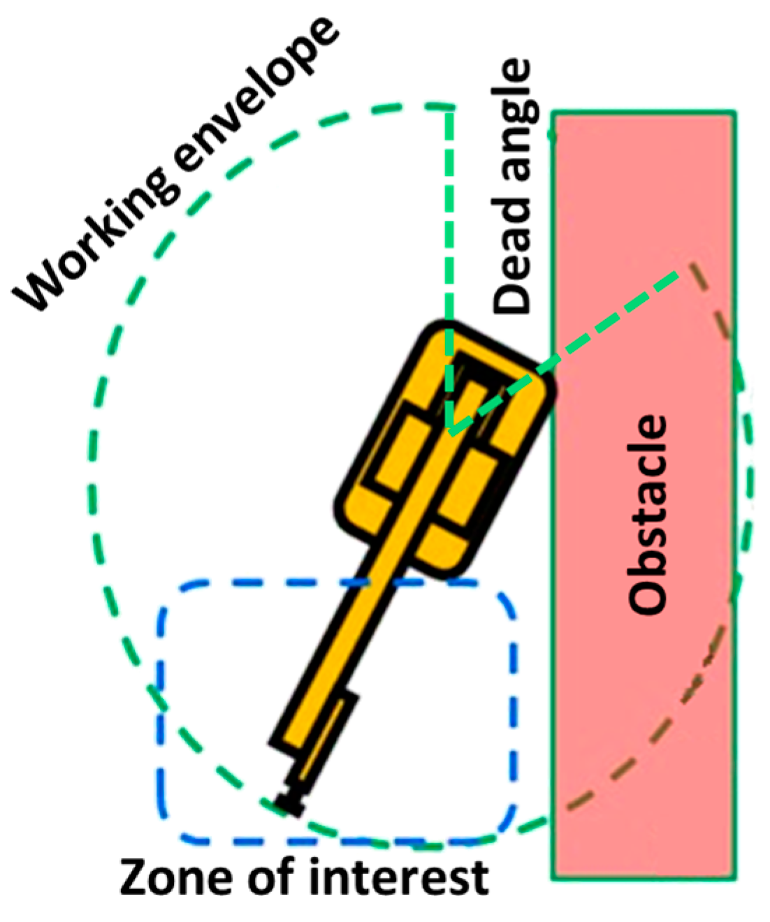
The physical restrictions of the workstation define the constraints of the optimization problem (e.g., invalid robot configurations, singularities, obstacles, etc.).

The idea is to link the decisional variables to the objective function through a set of decisional expressions represented by the robot inverse kinematic (IK) model [47,48,49,50]:

• ${\mathsf{\theta }}_j=f\left(\mathrm{P}i\right(\mathrm{x},\mathrm{y},\mathrm{z},\mathrm{R}\mathrm{x},\mathrm{R}\mathrm{y},\mathrm{R}\mathrm{z}\left)\right)$, $j=1, \dots , \mathrm{n}\mathrm{o}.\mathrm{o}\mathrm{f}\mathrm{d}.\mathrm{o}.\mathrm{f}=\mathrm{d}\mathrm{i}\mathrm{m} (\mathrm{j}\mathrm{o}\mathrm{i}\mathrm{n}\mathrm{t} \mathrm{s}\mathrm{p}\mathrm{a}\mathrm{c}\mathrm{e} \mathrm{q}=\mathsf{\theta })$
• Denavit-Hartenberg (DH) parameters of the robot manipulator [41,51]
• Robot working configuration in each point of interest on the robot trajectory,

where: i = 1…number of robot points of interest in the motion sequence, θ_j is the value of joint j, Pi is the location (position and orientation) to be reached by the robot in the point of interest i, and the DH parameters depend on the joint types, the transmission elements, and the physical dimensions of robot links. For the further analysis, P0 represents the ‘safe’ robot point from which the motion starts and where it ends (the global path is closed).

A graphical illustration of the trajectory is given in Figure 6. Both the desired points (fixed, modelled as input data) and the robot placement (variable, modelled as decisional variables) are expressed in the World Coordinate System (WCS). Inverse kinematics are computed for the relative position of the points of interest in the robot coordinate system (RCS) to determine the individual motions of each joint; then, the individual joint motions are transformed, using the robot EC model, into the total EC for the given trajectory.

The optimization problem is formulated as follows: given the position of the points of interest, the motion sequence and its parameters, and the type of robot, it is requested to compute the location of the robot base relative to the served points of interest so that the EC of the robot is minimized. The optimization problem is described in terms of data, decision variables and expressions, objective function, and constraints [52]. For optimization-specific robot placement, these elements are further detailed:

The data declaration represents the input information for the optimization model. It is composed of:

i

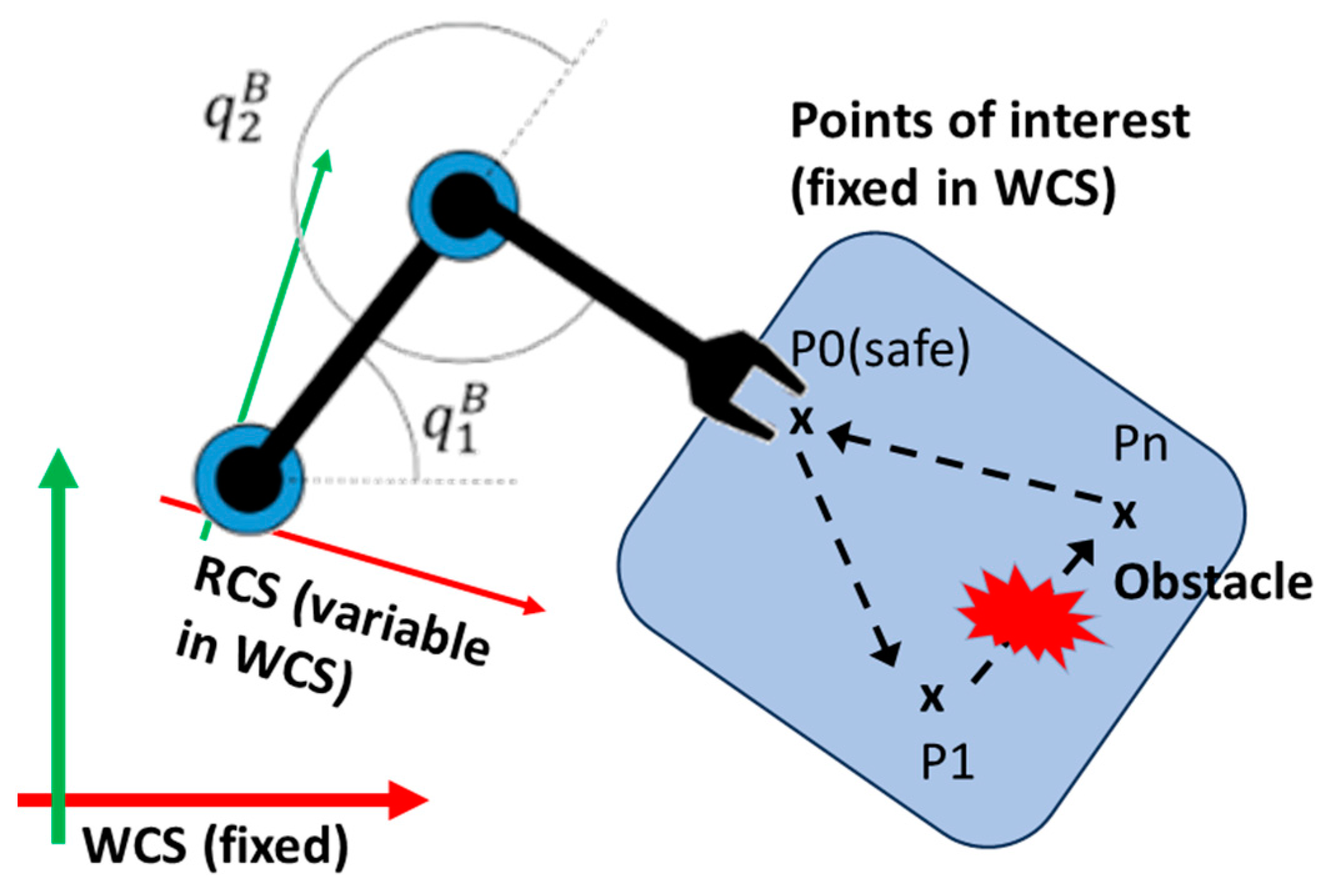
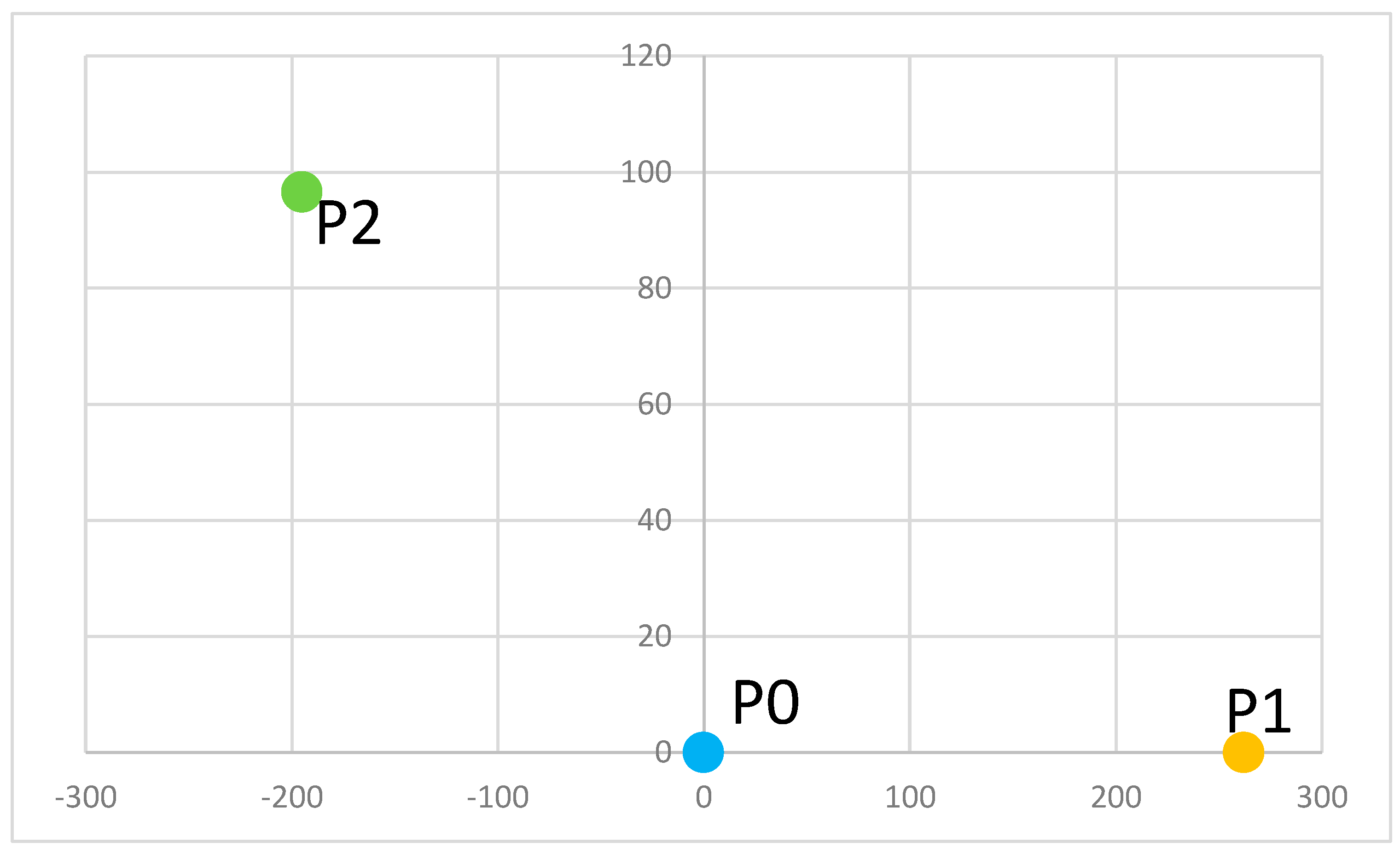
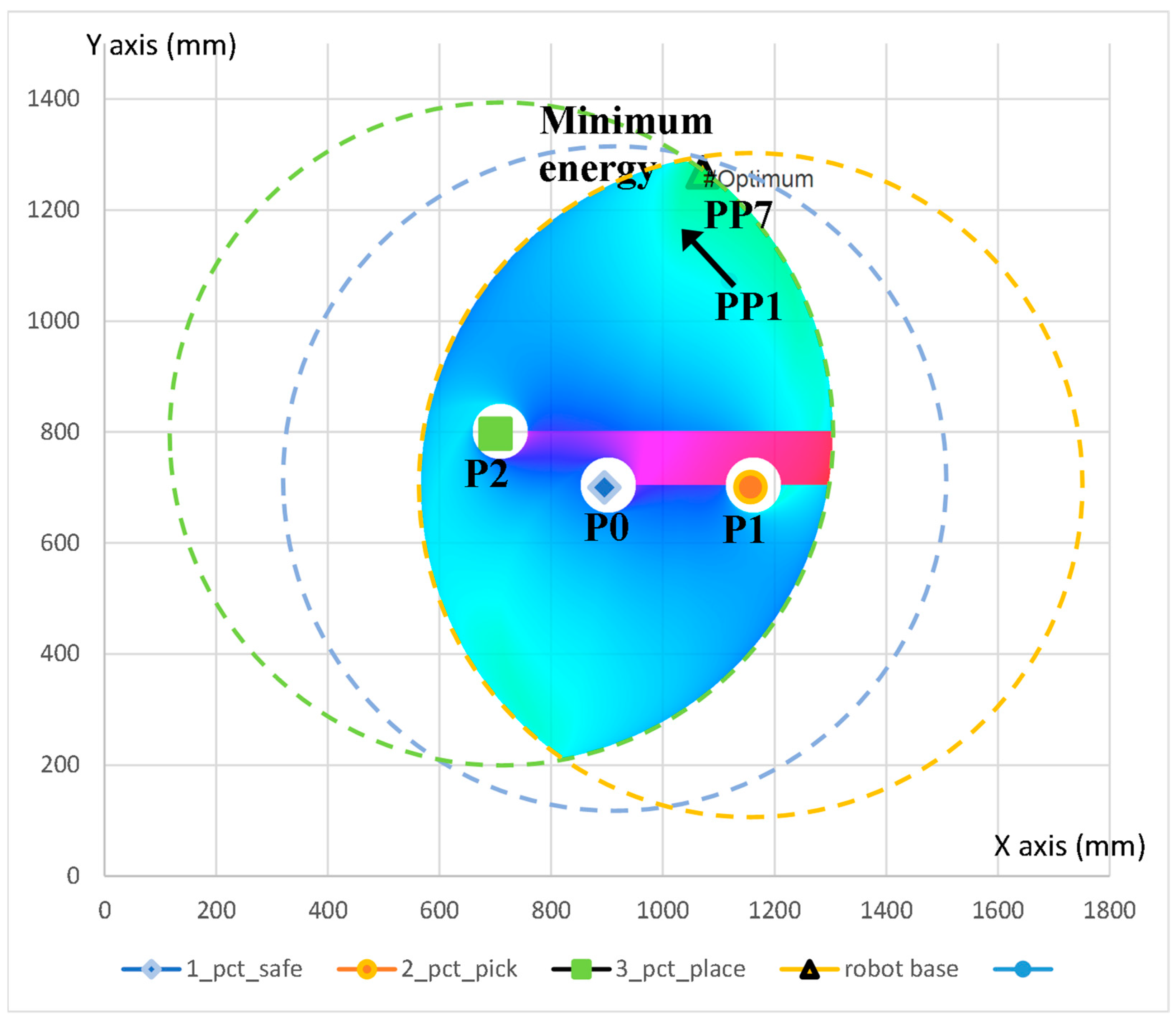
The position and orientation of the trajectory points of interest expressed in the WCS – $\mathrm{P}i(\mathrm{x},\mathrm{y},\mathrm{z},\mathrm{R}\mathrm{x},\mathrm{R}\mathrm{y},\mathrm{R}\mathrm{z}), i=1\dots n$, n being the total number of points. In the present analysis, a minimum number of three interest points is considered for a pick-and-place motion sequence, where P0 is the safe position where the robot waits for cycle code, P1 is the picking position where the robot picks the object to be handled, and P2 is the placing position where the robot releases the object [39].

ii

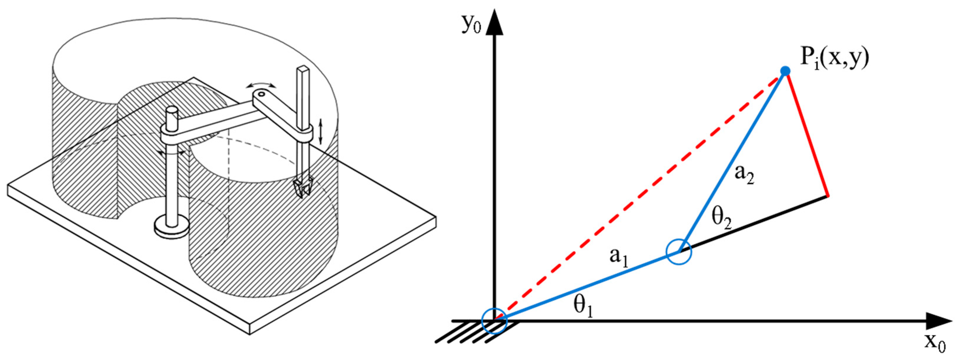
The robot type (e.g., SCARA, vertical articulated, etc.), which defines the types and succession of simple joints (prismatic or revolute).

iii

The Denavit-Hartenberg parameters of the robot, depending on the dimensions (length) and relative orientation (twist angle) of its segments.

iv

The robot EC model used to transform motion data into energy information. Items ii and iii contribute to the computation of the IK function $f\left(\mathrm{P}i\right)$ previously introduced, that expresses the robot points of interest from the WCS to the robot internal variables (joint) space.

The decision variables represent the position of the RCS relative to the WCS: position (x_rob, y_rob, z_rob) and orientation (Rx_rob, Ry_rob, Rz_rob) of the robot base segment. Based on the decision variables, the internal joint variables will be computed using decisional expressions for each point of interest ($\mathrm{P}i, i=1\dots n$): ${\theta }_j^{Pi}=f({\mathrm{x}\_\mathrm{r}\mathrm{e}\mathrm{l} }^{\mathrm{P}i},{\mathrm{y}\_\mathrm{r}\mathrm{e}\mathrm{l}}^{\mathrm{P}i},{\mathrm{z}\_\mathrm{r}\mathrm{e}\mathrm{l}}^{\mathrm{P}i},$ ${\mathrm{R}\mathrm{x}\_\mathrm{r}\mathrm{e}\mathrm{l}}^{\mathrm{P}i},{\mathrm{R}\mathrm{y}\_\mathrm{r}\mathrm{e}\mathrm{l}}^{\mathrm{P}i},{\mathrm{R}\mathrm{z}\_\mathrm{r}\mathrm{e}\mathrm{l}}^{\mathrm{P}i})$ where ${\mathrm{x}\_\mathrm{r}\mathrm{e}\mathrm{l}}^{Pi}$ and ${\mathrm{R}\mathrm{x}\_\mathrm{r}\mathrm{e}\mathrm{l}}^{Pi}$ respectively represent the position on x and rotation about x of the frame attached in point Pi expressed in RCS. The decisional expressions are dependent of the robot type (e.g., SCARA, vertical articulated, etc.).

The objective function represents the minimization of the total energy represented as a function of the total distance covered by all joints for the complete application path.

In all industrial applications the robot trajectory is a closed route which starts from a standard point defined as the ‘safe’ position (or loop-start point) and has a set of intermediate points resulting from the task specification (points of interest), the movement specification (intermediary points resulting from trajectory planning as is the case for linear movements in the WCS), and a set of fly-by points (needed to avoid obstacles). The number of intermediate points can vary from a small set of points for simple pick-and-place applications characterized by joint movements to a large set of points for complex trajectories characterized by both joint and linear/circular movements [12,53]. These points must be reached successively by the robot from P0 to Pn and back to P0; P0 is the ‘safe’ location where the robot waits for a cycle code.

Thus, the objective function is defined as the sum of all joint displacements between successive points, each joint motion being weighted by its actuator EC factor and scaled by the fraction of speed calculated according to the ‘leading axis’ principle that makes all joint motions start and stop simultaneously for the robot motion between any two successive points of interest $\mathrm{P}i,\mathrm{P}i+1$ (see Figure 3, right). Thus, joint velocity limitations are computed for each motion segment $\overline{\mathrm{P}i,\mathrm{P}i+1}$ by scaling down the robot cruise speed assigned to the ‘leading axis’ (the robot axis that travels the longest distance for that motion segment) with the ratio between the displacements of the current axis and of the leading axis (see the computational example in Table 2).

Hence, the computational model of the total EC cost of robot motion is expressed in Equation (1):

$$Total cost=\sum _{j=1}^{number of joints}\left[\left(\sum _{i=0}^n\left({\theta }_j^{P_{i+1}}-{\theta }_j^{P_i}\right)+{\theta }_j^{P_1}-{\theta }_j^{P_n}\right)\ast \left({joint}_j consumption weight\right)\ast ({joint}_j speed limitation) \right]$$

(1)

where: n is the total number of points of interest according to Figure 6 (the ‘safe’ robot position P0 is considered separate from the points of interest); θ_j is the value of joint j for reaching point Pi; joint_j consumption weight represents the unitary EC for 1 degree of moment of joint j; and joint_j speed limitation is the reduction in speed for any non-leading (non-dominant) axis. The total cost thus represents the total EC for a closed trajectory.

The constraints of the optimization problem involve zones and points in the search space which are not valid due to limitations of the working envelope (e.g., most types of industrial robots can rotate the first joint less than 360 degrees (Figure 7)) and obstacles such as other manufacturing resources, security fences, etc., as depicted in Figure 6 and Figure 7. Singular points are taken into consideration by the optimization solution. There are two types of singularities: frontier and internal. Frontier singularities are avoided by imposing constraints on the location of points of interest relative to the robot base. As for internal singularities, these are reflected with high EC into the objective function and hence eliminated from the optimized set. Since we consider only the first two links of the SCARA robot arm (placement of the control point) executing joint movements, we do not encounter such situations.

The theoretical problem is characterized by a large search space (six decision variables which have real values: position and orientation), a large number of points of interest Pi (which form the constraints of the problem) and nonlinear and complex functions to express decisional variables [54,55,56,57,58]. Since the interest is on minimizing EC, which is greatly influenced by the consumption of the robot arm (positioning of the arm end point, without orientation that features much less EC), the generic optimization problem can be reduced to a simplified form for the standard types of open kinematic (serial) industrial robots.

Because the optimization problem will be used in engineering applications (the outcome of the optimization is materialized by fastening the robot in the resulting location within its workspace – a complex task, prone to error because of the manipulator’s weight, which can be >800 kg, as in the case of ABB IRB6600 arms) it makes sense to further reduce the search space for the optimal solution by approximating the positioning values to integers representing millimetres.

In the following section, the simplified optimization model for SCARA-type robots with 2-link horizontally articulated mechanism and simple revolute joints will be presented (see Figure 8).

This simplified model of the EC optimization problem is justified by the fact that the actuators of the first two joints of an industrial robot have the largest share in the global EC of an industrial robot, regardless of its kinematic structure—anthropomorphic, SCARA, and others. In this simplified optimization model, the decisional variables are computed as integers representing millimetres, and all the robot points of interest $\mathrm{P}1, \dots , \mathrm{P}n$ are in the same Z plane being reached by the controlled end tip point through rotations of the two joints.

4. Localization of the Points of Interest in the WCS

This section describes the method used to digitize and position the points of interest along the robot trajectory within the WCS, starting from their relative position in the physical space. The relative positions of the points of interest are measured on the physical system, after which the algorithm described below will be applied for their positioning in the WCS.

Step 1: Measure the distances between the physical points of interest and store the resulting data as shown in

Table 3. Relative location of robot points of interest in the physical space.

#Point	Description	Distance Value (mm)
1	d01: Safe→P1	d01
2	d02: Safe→P2	d02
	…
n	d0n: Safe→Pn	d0n
N + 1	d12: P1→P2	d12
	…
n + n – 1	d1n: P1→Pn	d1n

.

Step 2: P0→P1 is the X axis, the Z axis is normal to the XOY plane, and OY is chosen according to the right-hand rule: P0 has coordinates (0,0), P1 has coordinates (d01,0).

Step 3: with the cosine theorem, locate the points P2…Pn in the coordinate system determined in Step 2. Out of the two possible locations for points 2…n, the one corresponding to the physical layout will be chosen. For the practical problem addressed in this paper, three points will be considered (safe position—P0, pick position—P1, place position—P2), and Table 3 will be customized as described in

Table 4. Relative location of the three points of interest in the physical space for the considered problem.

#Point	Description	Distance Value (mm)
1	d01: Safe→P1	262
2	d02: Safe→P2	217
3	d12: P1→P2	467

.

Based on these values, the following positions will result (Figure 9):

Step 4: choose a specific robot class for the application; depending on the class of the robot, a working envelope results and also implicitly an area where the robot can be positioned relative to each point of interest.

Step 5: The points P0→Pn are translated so that the optimization problem operates in the positive quadrant (X+, Y+): the minimum values for X and Y are chosen, then each point P0…n is offset by the same values on X and Y so that all points are in the positive quadrant (see Figure 10). For the practical problem addressed in this paper with a robot having a workspace radius of 600 mm (Adept Cobra S600), the offsets will be 600 mm (to the working envelope) + 100 mm (safety value) + 195 mm (position X of point P2) on X, and respectively 600 mm (working envelope) + 100 mm (safety value) + 0 mm (position Y of points ‘safe’ and P1) on Y.

Step 6: The optimization procedure described in Step 3 is called and the position of the robot base point is obtained.

Step 7: With the position of the base point, the relative distance of this point to the points of interest is calculated; in this way the robot will be placed in the physical space. Because for most industrial robots modelled as open kinematic chains the working envelope has an inaccessible area (behind the robot, see Figure 7 and Figure 8 left), the X axis is placed so that the points of interest are in the accessible zone.

5. Case Study

The resource on which the experiments were conducted is an Adept Cobra S600 SCARA robot with a two-link positioning mechanism in a horizontal plane mechanism, link lengths $a1=325 \mathrm{m}\mathrm{m}$ and $a2=275 \mathrm{m}\mathrm{m}$ and the total reach of the arm of 600 mm.

A simple pick-and-place procedure was considered for analysis. The pick-and-place procedure is a common automation task in manufacturing and logistics. This procedure involves the robot picking up an object from one location and placing it in another location, considering constraints such as (a) collisions with objects from the environment and (b) delicate operations which require fixed paths. Due to the previously stated constraints, this procedure can be characterized by several fly-by points and only three final points: safe position (P0), picking position (P1), and placing position (P2). The points of interest for this handling procedure are located in the local storage device and on the pallet transported by the conveyor.

The described research considers these points as fixed final points, and the robot should be placed in an optimized fashion relative to them. In this respect, a World Coordinate System (WCS) will be defined for the workstation where both fixed and variable points will be expressed. Using the relative position of the pick (P1), place (P2), and safe (P0) points, the WCS is defined in such a manner that all points of interest, including the possible positions of the robot base (as a function of its segments of lengths a1 and a2), are located in the positive quadrant:

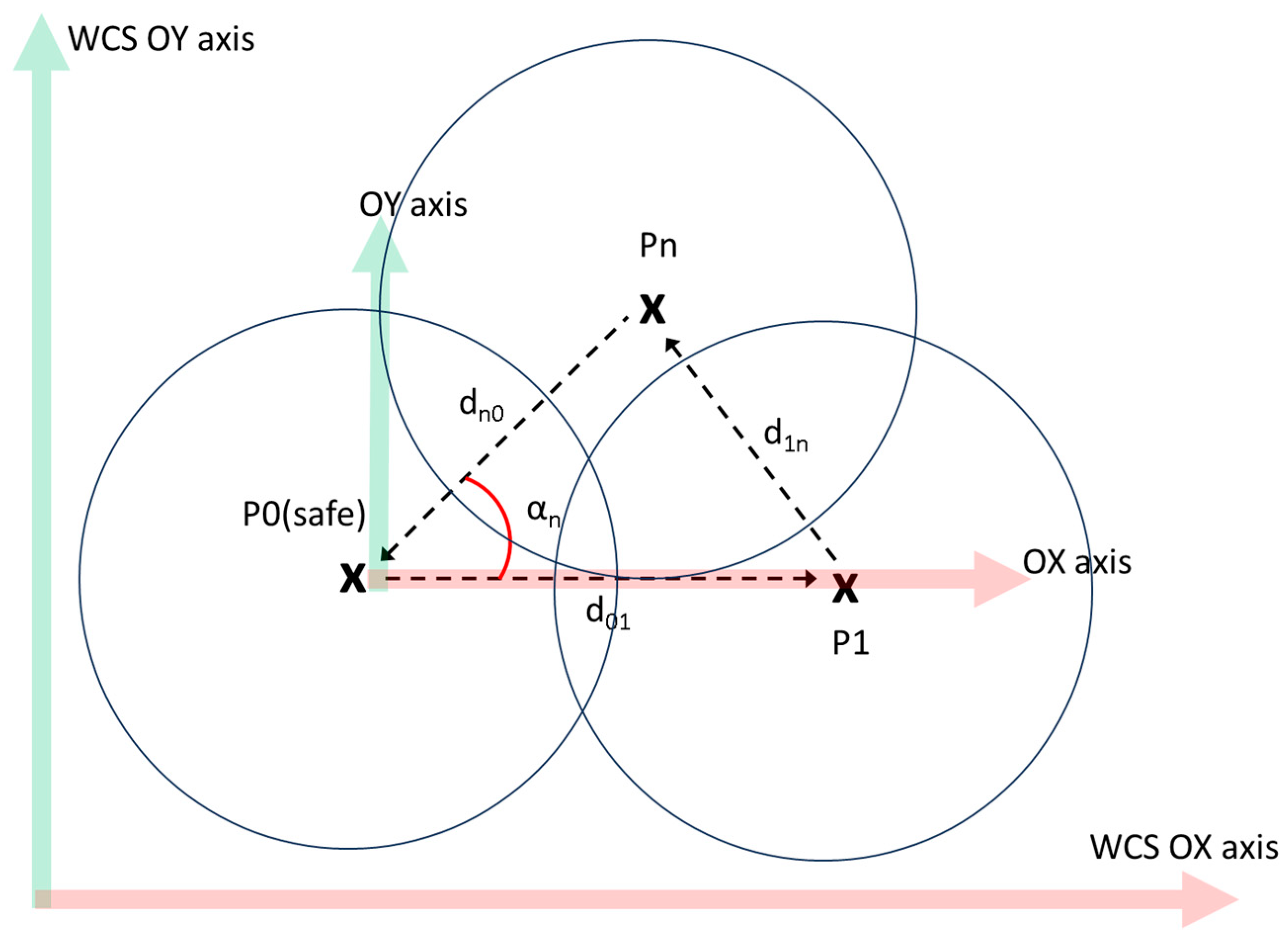
• The reverse robot working envelope (RRWE) is defined for each point of interest (a circle in the case of the two-link mechanism with the radius being the sum of the two link lengths: a1 + a2).
• The intersection of all RRWE is the search space of the optimization problem.
• The lower and left bounds are the locations of the WCS axes.

This process is described in Figure 11. The blue (safe—P0), orange (pick—P1), and green (place—P2) circles represent the possible positions of the robot base in order to reach the specific point. The search space is constructed with the data used in the steps presented in Section 4.

Based on the above assumptions, for a SCARA industrial robot, the values of the joint variables as a function of the XY position of the end-effector (considering only one operating configuration) are given by the equations:

$${\theta }_2=\pm \mathrm{acos}\left(\frac{x^2+y^2-a_1^2-a_2^2}{2a_1{a}_2}\right)$$

(2)

$${\theta }_1=atan\left(\frac{y}{x}\right)\mp atan\left(\frac{a_2\sin \left({\theta }_2\right)}{a_1+a_2\cos \left({\theta }_2\right)}\right)$$

(3)

These formulas are used to link the fixed positions of the pick-and-place procedure to the variable position of the robot base in the XY plane of the WCS. The computed joint variables will be further used to calculate the objective function. The weight of each joint is the energy consumed for a unit movement (Wsec/degree), from which the total energy consumed to complete the pick-and-place procedure results.

In this context, the objective is to determine the best position of the robot base which minimizes the EC when executing the 3-segment trajectory P0→P1→P2→P0. The problem, as formulated above, is an optimization problem characterized by:

(a)

Input data for the optimization engine (known values): positions (P0…2), robot dimensions (a1, a2), and robot configuration (θ₂ positive, + sign in Equation (2) and − sign in Equation (3)) meaning a righty configuration).

(b)

Decisional variables: position of the robot base ($x_{rob}$, $y_{rob}$).

(c)

Decision expressions computed using Equations (2) and (3): values of the joints for each point of the pick-and-place procedure ${\mathsf{\theta }}_1^{\mathrm{P}1\dots \mathrm{P}3},{\mathsf{\theta }}_2^{\mathrm{P}1\dots \mathrm{P}3}$.

(d)

The optimization function which should be minimized: total energy, as defined in Equation (1).

(e)

Constraints: the position of the robot base is an integer in the intervals [500 mm, 1300 mm] for the X axis and [200 mm, 1300 mm] for the Y axis (see Figure 11).

Based on these numerical values, an optimization model was developed using the Excel Solver engine which employs the generalized reduced gradient (GRG) method which is adequate for the nonlinear structure of the equation describing the decisional expressions (inverse kinematics). The GRG algorithm adjusts the variables of the function to find the optimal solution by considering the gradients (or rates of change) of the objective function and the constraints, making it effective for problems where the relations between variables are not linear. Possible robot placements without IK solutions have been excluded using the IFERROR Excel function which returns a maximum energy value outside the range of possible energy values defined for this project. The result is depicted in Figure 12.

The runtime of the optimization model implemented in Excel Solver using GRG nonlinear is 96 s, yielding a minimum energy of 67 Wsec. Alternatively, the whole search space was computed and plotted (Figure 13). From the graphical representation it can be observed that the minimum is in a zone (green) of minimum energy, which is good from a practical point of view because it is difficult to precisely position the robot base with mm accuracy.

In the second part of the experiment, tests were conducted to measure the actual EC for a similar system. Because the robot base was fixed in this case (Figure 2), the pick-and-place procedure was carried out using variable final points, simulating different placements of the robot. In this case, the locations of P1, P2, and P0 started from the values described in Table 3 and were all translated with 10 mm away from the robot (in the direction of the black arrow in Figure 11). From Figure 11 and Figure 13, it can be observed that the farther away the robot base is, the lower is the EC, which complies with the search space colour notation (green—low: EC $<$100 Wsec; light blue—medium: EC $\in (100 \mathrm{W}\mathrm{s}\mathrm{e}\mathrm{c},250 \mathrm{W}\mathrm{s}\mathrm{e}\mathrm{c})$, purple—high: $\mathrm{E}\mathrm{C}\in (250 \mathrm{W}\mathrm{s}\mathrm{e}\mathrm{c},500 \mathrm{W}\mathrm{s}\mathrm{e}\mathrm{c})$, red—very high: $\mathrm{E}\mathrm{C}>500 \mathrm{W}\mathrm{s}\mathrm{e}\mathrm{c}$.

6. Conclusions and Future Research Direction

This article has investigated how robot placement influences the total EC for a simple material-handling procedure performed by industrial robots—pick-and-place. An IED-based smart meter was developed to analyse instantaneous power absorption for both individual joint motions and robot trajectory. These data were used to develop an EC model for a specific robot type—the SCARA Cobra S600 robot from Adept. A simplified optimization model was implemented using input data previously collected from the energy meter. The optimization model was then validated through comparison with the EC measured during the execution of the pick-and-place procedure.

Although the evaluation and calculation of EC in a real scenario (all actuators for the robot arm with end-effector, all intermediate points, linear movements in Cartesian, and environment constraints for both the controlled point (the end-tip point) and the robot links) require an important modelling and calculation effort, the reported research shows that an intelligent positioning of the robot base can bring advantages in terms of energy consumed. A visual description of the search space (distribution of EC, see Figure 7) helps because the robot mounting position is decided to a considerable degree by the physical constraints of the application and has limited precision in comparison with the mathematical model. Thus, finding zones of reduced consumption is better than going for the global optimum. Alternatively, different optimization criteria can be followed, such as the balanced use of motors to avoid situations in which one of the robot axes fails due to intensive wear of its actuator.

Being implemented in the design stage of a manufacturing workstation’s layout, the benefits of the proposed method consist of providing a base level of EC saving over the entire lifecycle of industrial robots working in a known environment, to which energy-saving features and trajectory parameter adjustments can be further added in the context of application variance (e.g., changes in the weight of handled parts, accessing moving parts, planning robot motion with vision system, etc.)

Further development directions are considered:

(a)

Increasing the complexity of the model by considering all degrees of freedom, increasing the decision variables from placement in the XY plane to placement in the operational space (XYZ and rotation, usually over Z), increasing the number of fly-by points as this is the case for real scenarios, considering linear motion paths in the operational space, and accounting for possible collisions of the robot segments with workplace equipment.

(b)

Analysing how the alternation between mechanical brakes and servo brakes influences the EC in the situations when the equipment is not used, e.g., the robot is waiting for a pallet to arrive in the workstation.

(c)

Adjusting the speed according to the workload of the workstation: if the work queue is full, the robot operates at a lower speed, reducing EC.

References

1. IEA (International Energy Agency). World Energy Outlook 2022. 2022. Available online: https://www.iea.org/reports/world-energy-outlook-2022 (accessed on 12 October 2023).
2. Müller, C. World Robotics 2022—Industrial Robots, IFR Statistical Department, VDMA Services GmbH, Frankfurt am Main, Germany. 2022. Available online: https://ifr.org/img/worldrobotics/Executive_Summary_WR_Industrial_Robots_2022.pdf (accessed on 17 December 2023).
3. Fujimori, S.; Matsuoka, Y. Development of method for estimation of world industrial energy consumption and its application. Energy Econ. 2011, 33, 461–473. [Google Scholar] [CrossRef]
4. Binderbauer, P.J.; Woegerbauer, M.; Nagovnak, P.; Kienberger, T. The effect of “energy of scale” on the energy consumption in different industrial sectors. Sustain. Prod. Consum. 2023, 41, 75–87. [Google Scholar] [CrossRef]
5. Olanrewaju, O.; Jimoh, A.; Kholopane, P. Integrated IDA–ANN–DEA for assessment and optimization of energy consumption in industrial sectors. Energy 2012, 46, 629–635. [Google Scholar] [CrossRef]
6. Pellicciari, M.; Berselli, G.; Leali, F.; Vergnano, A. A method for reducing the energy consumption of pick-and-place industrial robots. Mechatronics 2013, 23, 326–334. [Google Scholar] [CrossRef]
7. Othman, A.; Belda, K.; Burget, P. Physical modelling of energy consumption of industrial articulated robots. In Proceedings of the 2015 15th International Conference on Control, Automation and Systems (ICCAS), Busan, Republic of Korea, 13–16 October 2015; pp. 784–789. [Google Scholar]
8. Zhao, G.; Liu, Z.; He, Y.; Cao, H.; Guo, Y. Energy consumption in machining: Classification, prediction, and reduction strategy. Energy 2017, 133, 142–157. [Google Scholar] [CrossRef]
9. McKerracher, C.; Torriti, J. Energy consumption feedback in perspective: Integrating Australian data to meta-analyses on in-home displays. Energy Effic. 2013, 6, 387–405. [Google Scholar] [CrossRef]
10. Babiuch, M.; Foltynek, P.; Smutny, P. Using the ESP32 Microcontroller for Data Processing. In Proceedings of the 2019 20th International Carpathian Control Conference (ICCC), Krakow, Poland, 26–29 May 2019; pp. 1–6. [Google Scholar]
11. Zhang, M.; Yan, J. A data-driven method for optimizing the energy consumption of industrial robots. J. Clean. Prod. 2020, 285, 124862. [Google Scholar] [CrossRef]
12. Soori, M.; Arezoo, B.; Dastres, R. Optimization of energy consumption in industrial robots, a review. Cogn. Robot. 2023, 3, 142–157. [Google Scholar] [CrossRef]
13. Kim, S.; Jin, H.; Seo, M.; Har, D. Optimal Path Planning of Automated Guided Vehicle using Dijkstra Algorithm under Dynamic Conditions. In Proceedings of the 2019 7th International Conference on Robot Intelligence Technology and Applications (RiTA), Daejeon, Republic of Korea, 1–3 November 2019; pp. 231–236. [Google Scholar]
14. Paes, K.; Dewulf, W.; Elst, K.V.; Kellens, K.; Slaets, P. Energy Efficient Trajectories for an Industrial ABB Robot. Procedia CIRP 2014, 15, 105–110. [Google Scholar] [CrossRef]
15. Aggogeri, F.; Borboni, A.; Pellegrini, N. Jerk Trajectory Planning for Assistive and Rehabilitative Mechatronic Devices. Int. Rev. Mech. Eng. (IREME) 2016, 10, 543. [Google Scholar] [CrossRef]
16. Omron. eV+Language Reference Guide, v2.x, 18319–000 Rev A, Omron Adept Technologies. 2016, pp. 138–141. Available online: https://assets.omron.eu/downloads/manual/en/v3/i605_ev%2B_language_reference_manual_en.pdf (accessed on 17 December 2023).
17. Yamamoto, T.; Hayama, H.; Hayashi, T.; Mori, T. Automatic Energy-Saving Operations System Using Robotic Process Automation. Energies 2020, 13, 2342. [Google Scholar] [CrossRef]
18. Mura, M.D.; Dini, G. Designing assembly lines with humans and collaborative robots: A genetic approach. CIRP Ann. 2019, 68, 1–4. [Google Scholar] [CrossRef]
19. Vodovozov, V.; Raud, Z.; Petlenkov, E. Review on Braking Energy Management in Electric Vehicles. Energies 2021, 14, 4477. [Google Scholar] [CrossRef]
20. Meike, D.; Ribickis, L. Recuperated energy savings potential and approaches in industrial robotics. In Proceedings of the 2011 IEEE International Conference on Automation Science and Engineering (CASE 2011), Trieste, Italy, 24–27 August 2011; pp. 299–303. [Google Scholar]
21. Palomba, I.; Wehrle, E.; Carabin, G.; Vidoni, R. Minimization of the Energy Consumption in Industrial Robots through Regenerative Drives and Optimally Designed Compliant Elements. Appl. Sci. 2020, 10, 7475. [Google Scholar] [CrossRef]
22. Wu, F.; Howard, M. Energy Regenerative Damping in Variable Impedance Actuators for Long-Term Robotic Deployment. IEEE Trans. Robot. 2020, 36, 1778–1790. [Google Scholar] [CrossRef]
23. Yaskawa Europe. Yaskawa Robots with Regenerative Braking. Energy-Efficient Robots. 2022. Available online: https://www.yaskawa.eu.com/header-meta/news-events/article/yaskawa-robots-with-regenerative-braking_n18865 (accessed on 17 December 2023).
24. Yin, S.; Ji, W.; Wang, L. A machine learning based energy efficient trajectory planning approach for industrial robots. Procedia CIRP 2019, 81, 429–434. [Google Scholar] [CrossRef]
25. Nonoyama, K.; Liu, Z.; Fujiwara, T.; Alam, M.; Nishi, T. Energy-Efficient Robot Configuration and Motion Planning Using Genetic Algorithm and Particle Swarm Optimization. Energies 2022, 15, 2074. [Google Scholar] [CrossRef]
26. Gorkavyy, M.A.; Gorkavyy, A.I.; Egorova, V.P.; Melnichenko, M.A. Automated method based on a neural network model for searching energy-efficient complex movement trajectories of industrial robot in a differentiated technological process. Front. Energy Res. 2023, 11, 1129311. [Google Scholar] [CrossRef]
27. Schmidt, C.; Li, W.; Thiede, S.; Kara, S.; Herrmann, C. A methodology for customized prediction of energy consumption in manufacturing industries. Int. J. Precis. Eng. Manuf. Technol. 2015, 2, 163–172. [Google Scholar] [CrossRef]
28. Lin, H.-I.; Mandal, R.; Wibowo, F.S. BN-LSTM-based energy consumption modeling approach for an industrial robot manipulator. Robot. Comput. Manuf. 2024, 85, 102629. [Google Scholar] [CrossRef]
29. Morariu, C.; Morariu, O.; Răileanu, S.; Borangiu, T. Machine learning for predictive scheduling and resource allocation in large scale manufacturing systems. Comput. Ind. 2020, 120, 103244. [Google Scholar] [CrossRef]
30. Rubio, F.; Llopis-Albert, C.; Valero, F. Multi-objective optimization of costs and energy efficiency associated with autonomous industrial processes for sustainable growth. Technol. Forecast. Soc. Chang. 2021, 173, 121115. [Google Scholar] [CrossRef]
31. Guerra-Santin, O.; Itard, L. The effect of energy performance regulations on energy consumption. Energy Effic. 2012, 5, 269–282. [Google Scholar] [CrossRef]
32. da Cunha, C.; Cardin, O.; Gallot, G.; Viaud, J. Designing the Digital Twins of Reconfigurable Manufacturing Systems: Application on a smart factory. IFAC-PapersOnLine 2021, 54, 874–879. [Google Scholar] [CrossRef]
33. Velchev, S.; Kolev, I.; Ivanov, K.; Gechevski, S. Empirical models for specific energy consumption and optimization of cutting parameters for minimizing energy consumption during turning. J. Clean. Prod. 2014, 80, 139–149. [Google Scholar] [CrossRef]
34. Luan, F.; Yang, X.; Chen, Y.; Regis, P.J. Industrial robots and air environment: A moderated mediation model of population density and energy consumption. Sustain. Prod. Consum. 2022, 30, 870–888. [Google Scholar] [CrossRef]
35. Răileanu, S.; Borangiu, T.; Anton, F. Establishing Optimal Energy Working Parameters for a Robotized Manufacturing Cell. In Advances in Intelligent Systems and Computing; Springer: Cham, Switzerland, 2016; Volume 371. [Google Scholar] [CrossRef]
36. Qiu, B.; Chen, S.; Xiao, T.; Gu, Y.; Zhang, C.; Yang, G. A Feasible Method for Evaluating Energy Consumption of Industrial Robots. In Proceedings of the 2021 IEEE 16th Conference on Industrial Electronics and Applications (ICIEA), Chengdu, China, 1–4 August 2021; pp. 1073–1078. [Google Scholar]
37. Liu, A.; Liu, H.; Yao, B.; Xu, W.; Yang, M. Energy consumption modeling of industrial robot based on simulated power data and parameter identification. Adv. Mech. Eng. 2018, 10, 1687814018773852. [Google Scholar] [CrossRef]
38. Barai, G.R.; Krishnan, S.; Venkatesh, B. Smart metering and functionalities of smart meters in smart grid—A review. In Proceedings of the 2015 IEEE Electrical Power and Energy Conference (EPEC), London, ON, Canada, 26–28 October 2015; pp. 138–145. [Google Scholar]
39. Narayan, S.; Doytch, N. An investigation of renewable and non-renewable energy consumption and economic growth nexus using industrial and residential energy consumption. Energy Econ. 2017, 68, 160–176. [Google Scholar] [CrossRef]
40. Tauber, M.; Skopik, F.; Bleier, T.; Hutchison, D. A Self-Organising Approach for Smart Meter Communication Systems. In Lecture Notes in Computer Science; Springer: Berlin/Heidelberg, Germany, 2013; Volume 8221. [Google Scholar] [CrossRef]
41. Siciliano, B.; Sciavicco, L.; Villani, L.; Oriolo, G. Robotics: Modelling, Planning and Control; Springer Science & Business Media: Berlin/Heidelberg, Germany, 2010; ISBN 1846286417. [Google Scholar]
42. Yang, B.; Yang, W. Modular approach to kinematic reliability analysis of industrial robots. Reliab. Eng. Syst. Saf. 2022, 229, 108841. [Google Scholar] [CrossRef]
43. Gao, G.; Sun, G.; Na, J.; Guo, Y.; Wu, X. Structural parameter identification for 6 DOF industrial robots. Mech. Syst. Signal Process. 2017, 113, 145–155. [Google Scholar] [CrossRef]
44. Abdelkhalik, O.; Darani, S. Optimization of nonlinear wave energy converters. Ocean Eng. 2018, 162, 187–195. [Google Scholar] [CrossRef]
45. Dinh, Q.T.; Savorgnan, C.; Diehl, M. Adjoint-Based Predictor-Corrector Sequential Convex Programming for Parametric Nonlinear Optimization. SIAM J. Optim. 2011, 22, 1258–1284. [Google Scholar] [CrossRef]
46. Alam, M.; Ibaraki, S.; Fukuda, K.; Morita, S.; Usuki, H.; Otsuki, N.; Yoshioka, H. Inclusion of Bidirectional Angular Positioning Deviations in the Kinematic Model of a Six-DOF Articulated Robot for Static Volumetric Error Compensation. IEEE/ASME Trans. Mechatron. 2022, 27, 4339–4349. [Google Scholar] [CrossRef]
47. Game, R.U.; Davkhare, A.A.; Pakhale, S.S.; Ekhande, S.B.; Shinde, V.B. Kinematic analysis of various robot configurations. Int. Res. J. Eng. Technol. (IRJET) 2017, 4, 921–935. [Google Scholar]
48. Alam, M.; Ibaraki, S.; Fukuda, K. Kinematic Modeling of Six-Axis Industrial Robot and its Parameter Identification: A Tutorial. Int. J. Autom. Technol. 2021, 15, 599–610. [Google Scholar] [CrossRef]
49. Ma, L.; Bazzoli, P.; Sammons, P.M.; Landers, R.G.; Bristow, D.A. Modeling and calibration of high-order joint-dependent kinematic errors for industrial robots. Robot. Comput. Manuf. 2017, 50, 153–167. [Google Scholar] [CrossRef]
50. Zhou, J.; Nguyen, H.-N.; Kang, H.-J. Simultaneous identification of joint compliance and kinematic parameters of industrial robots. Int. J. Precis. Eng. Manuf. 2014, 15, 2257–2264. [Google Scholar] [CrossRef]
51. Toquica, J.S.; Oliveira, P.S.; Souza, W.S.; Motta, J.M.S.; Borges, D.L. An analytical and a Deep Learning model for solving the inverse kinematic problem of an industrial parallel robot. Comput. Ind. Eng. 2020, 151, 106682. [Google Scholar] [CrossRef]
52. Leyffer, S.; Menickelly, M.; Munson, T.; Vanaret, C.; Wild, S.M. A survey of nonlinear robust optimization. INFOR: Inf. Syst. Oper. Res. 2020, 58, 342–373. [Google Scholar] [CrossRef]
53. Anton, F.; Anton, S.; Borangiu, T.; Răileanu, S. Optimizing Trajectory Points for High Speed Assembly Operations. In Advances in Robot Design and Intelligent Control: Proceedings of the 24th International Conference on Robotics in Alpe-Adria-Danube Region (RAAD), Bucharest, Romania, 27–29 May 2015; Springer: Cham, Switzerland, 2015; Volume 371. [Google Scholar] [CrossRef]
54. D’Agostino, D.; Serani, A.; Campana, E.; Diez, M. Nonlinear Methods for Design-Space Dimensionality Reduction in Shape Optimization, Machine Learning, Optimization and Big Data (MOD 2017). In Lecture Notes in Computer Science; Springer: Berlin/Heidelberg, Germany, 2017; p. 10710. [Google Scholar] [CrossRef]
55. Abdi, M.; Ashcroft, I.; Wildman, R. Topology optimization of geometrically nonlinear structures using an evolutionary optimization method. Eng. Optim. 2018, 50, 1850–1870. [Google Scholar] [CrossRef]
56. Žilinskas, A.; Žilinskas, J. Interval Arithmetic Based Optimization in Nonlinear Regression. Informatica 2010, 21, 149–158. [Google Scholar] [CrossRef]
57. Blumensath, T. Compressed Sensing with Nonlinear Observations and Related Nonlinear Optimization Problems. IEEE Trans. Inf. Theory 2012, 59, 3466–3474. [Google Scholar] [CrossRef]
58. Zhou, J.; Yu, Y.; Liu, Y.; Zhang, Y. Solving nonlinear optimization problems with bipolar fuzzy relational equation constraints. J. Inequalities Appl. 2016, 2016, 126. [Google Scholar] [CrossRef]
Figure 1. Long short-term memory (LSTM) time sequence for energy consumption (EC) prediction with intermediate step comparison [29].
Sustainability 16 01053 g001
Figure 2. Robotized workstation automating a material-handling procedure.
Sustainability 16 01053 g002
Figure 3. Digital representation of a robot arm executing a joint movement between two points and the kinematics of joint 1 and 2 (joint position and speed profile).
Sustainability 16 01053 g003
Figure 4. Improved energy measurement customized in an Intelligent Embedded Device (IED).
Sustainability 16 01053 g004
Figure 5. Joint 1 100-degree movement back and forth with 80% speed limitation; average movement consumption is 73.25 Wsec resulting in an EC of 0.73 Wsec for 1 degree of movement.
Sustainability 16 01053 g005
Figure 6. Theoretical representation of the optimization problem.
Sustainability 16 01053 g006
Figure 7. Graphic representation of forbidden zones (obstacles) in the search space (robot working envelope).
Sustainability 16 01053 g007
Figure 8. Working envelope (left) and kinematic model (right) for a 2-link horizontally articulated (SCARA-type) robot arm.
Sustainability 16 01053 g008
Figure 9. Formation of the initial WCS and the location of the points of interest for the considered problem.
Sustainability 16 01053 g009
Figure 10. Formation of the WCS and localization of the input data.
Sustainability 16 01053 g010
Figure 11. Search space of the robot placement optimization problem. The EC is illustrated with colours ranging from green representing low EC (less than 100 Wsec) to purple and red representing high EC (more than 300 Wsec). The energy histogram is depicted in Figure 12.
Sustainability 16 01053 g011
Figure 12. Distribution of EC values of the search space from Figure 11.
Sustainability 16 01053 g012
Figure 13. Energy consumption for the pick-and-place procedure with variable robot placement: the relative distance of the points of interest is shifted from the base with 10 mm for each cycle (1→2→3→4→5→6→7) (black arrow in Figure 11).
Sustainability 16 01053 g013