Abstract
Coupling effects of various loading conditions can cause deflections, settlements and even failure of in-service bridges. Although it is one of the most critical loads, unfortunately, loading conditions of moving vehicles are difficult to capture in real time by bridge monitoring systems currently in place for sustainable operation. To fully understand the status of a bridge, it is essential to obtain instantaneous vehicle load distributions in a dynamic traffic environment. Although there are some methods that can identify overweight vehicles, the captured vehicle-related information is scattered and incomplete and thus cannot support effective bridge structural health monitoring (BSHM). This study proposes a noncontact, vision-based approach to identification of vehicle loads for real-time monitoring of bridge structural health. The proposed method consists of four major steps: (1) establish a dual-object detection model for vehicles using YOLOv7, (2) develop a hybrid coordinate transformation model on a bridge desk, (3) develop a multiobject tracking model for real-time trajectory monitoring of moving vehicles, and (4) establish a decision-level fusion model for fusing data on vehicle loads and positions. The proposed method effectively visualizes the 3D spatiotemporal vehicular-load distribution with low delay at a speed of over 30FPS. The results show that the hybrid coordinate transformation ensures that the vehicle position error is within 1 m, a 5-fold reduction compared with the traditional method. Wheelbase is calculated through dual-object detection and transformation and is as the primary reference for vehicle position correction. The trajectory and real-time speed of vehicles are preserved, and the smoothed speed error is under 5.7%, compared with the speed measured by sensors. The authors envision that the proposed method could constitute a new approach for conducting real-time SHM of in-service bridges.
1. Introduction
The loading conditions of moving vehicles, along with the loadings of wind, temperature, etc., cause constant deflections, strain and settlement of bridges, which can significantly affect the sustainability operation of bridges [1,2]. However, only vehicle counts and gross weight are incorporated into currently operating BSHM systems. These general vehicle data are coarse and uncorrelated and do not reflect the loading conditions of the vehicles on the bridge. The number and weight of vehicles are calculated at predetermined intervals, in contrast to the instantaneous measurement of other loading factors. Therefore, vehicle load is underspecified and underused as a parameter for analysis of structural performance under real-time traffic loading. To develop a sustainable and reliable infrastructure, it is essential to develop a real-time monitoring method that includes the calculation of multidimensional vehicle loads.
Weigh-in-motion systems (WIMs) are the classic method for direct sensing of vehicle loading. Based on continuous wheel measurements, WIMs overcome the problems of time consumption and inescapable installation cost associated with static weighting platforms. For this reason, they are widely used on bridges, where they provide verified desirable accuracy with relatively low operating costs [3,4,5]. Beyond such direct measurements, indirect methods using sensors have also been developed to acquire vehicle weights. This approach was derived from a theory of loading inversion that uses bridge-structure responses [6]. Examples include interpretive methods [7,8], a time-domain method [9] and a frequency-time-domain method [10]. Based on these methods, bridge weigh-in-motion systems (BWIMs), which measure wheel pressure via section strain on the bridge deck, were proposed [11]. New studies on BWIMs have continued to emerge, including Slovenian BWIM [12], fiber-optic-based BWIMs [13] and transmissibility-like index-based BWIMs [14]. Indirect methods take advantage of interpreting moving force identification (MFI) along the whole bridge desk. This method represents an extension of bridge vehicle loading identification research to the spatial dimension, compared to the limited loading information from WIMs. However, sensors used for capturing dynamic responses in structural behavior pick up high of noise due to structural vibrations and environmental factors, which affects the effectiveness of BWIMs [14].
As deep learning is being researched intensively in civil engineering, computer vision appears superiority in remote sensing for use in displacement measurement, crack evaluation and vibration monitoring [15,16,17]. The vision method provides a completely novel solution to contactless acquisition of spatial information and has the capability to eliminate environmental effects via increasingly sophisticated processing technology [18,19,20]. Template matching was used for vehicle detection with WIMs [21]. As a classical algorithm, template matching has its limitations in terms of the template sizes for different vehicle types. Binarization by the Gaussian mixture model was used to acquire vehicle locations [22]. While this image-processing method is size-free, it is easily impacted by light and shadow. Loading-distribution algorithms are supported by the development of object detection, which increases the speed and usability of contactless MFI. R-CNN and YOLO series are representative algorithms in this field, wherein innovative network structures such as SPPnet, FPN and PANnet are now playing a major role [23,24]. Zhang et al. explored how to obtain the length, axle number, speed and lane of moving vehicles using Faster R-CNN [25]. Obviously, this method was not comprehensive, as vehicle weight information was not included. In order to obtain data on loading, Kong and Feng proposed a noncontact weighing method that involved capturing vehicle tire images [26,27]. Zhu reconstructed a 3D bounding box for each vehicle using YOLOv5 and simulated the traffic data with historical records [28]. Although this research was innovative, there was problem of reliability with the loading data. Gan, Zhu and Ge used a vision method with other sensors to develop robust identification systems [29,30,31]. However, the precision and stability of the data will be enhanced by improvements to the detection algorithm.
Visual multiobject tracking (MOT) provides a temporal dimension based on the spatial distribution of vehicle loading by using object matching between different frames. Particle filtering involves sampling random points on detected objects to select the maximum-probability particle for tracking [21]. A Gaussian mixture model was used to reduce image background noise and eliminate the interference of the tracking environment during object matching [22]. Unlike detection-point tracking, the updated algorithms, such as Simple Online and Realtime Tracking (SORT) and DEEPSORT [32,33], make maximum use of the visual data on the vehicles and take the attributes from the object bounding box as the state predictions of the Kalman filter to ensure the accuracy of vehicle matching. Although high-precision nonlinear methods have also been imported in tracking, these filtering methods involve complicated calculations.
According to the reviewed literature, there are still three salient points worthy of attention on the subject of real-time, multidimensional vehicle load identification. The primary point is the acquisition of vehicle weight data. In many publications, gross vehicle weight (GVW) was obtained from historical statistical data, and a loading value was estimated by averaging these weights. Although the accuracy of these statistical correlations has been roughly confirmed, some overloaded vehicles might be missing from the real-time loading data, and the identification of such vehicles is crucial for bridge monitoring. Secondly, some methods are more focused on redundant vehicle information than on precise measures of loading location. In particular, some means of coordinate transformation do not achieve expectations, which impacts the precision of loading-distribution analyses. The last point is that most methods for monitoring vehicle loading are static and cause delays in traffic flow, while the long-term trend of BSHM is towards rapid response and smooth flow of traffic. However, indirect measurements and simulation models of MFI have drawbacks in terms of authenticity and efficiency. Regarding these points, this study combines WIMs and vision technology to generate a dynamic, realistic loading-distribution model. Through developing low-latency detection, MOT algorithms and an innovative image-calibration method, a real-time spatiotemporal monitoring method of bridge vehicle loading is proposed.
The remaining sections in this study are structured as follows: the framework of the proposed method is introduced in Section 2; the methodology is described in Section 3; Section 4 explains the case study, including preparation, verification of the hybrid calibration model and field tests of the proposed method; and the conclusion and aims of future work are covered in Section 5.
2. Framework
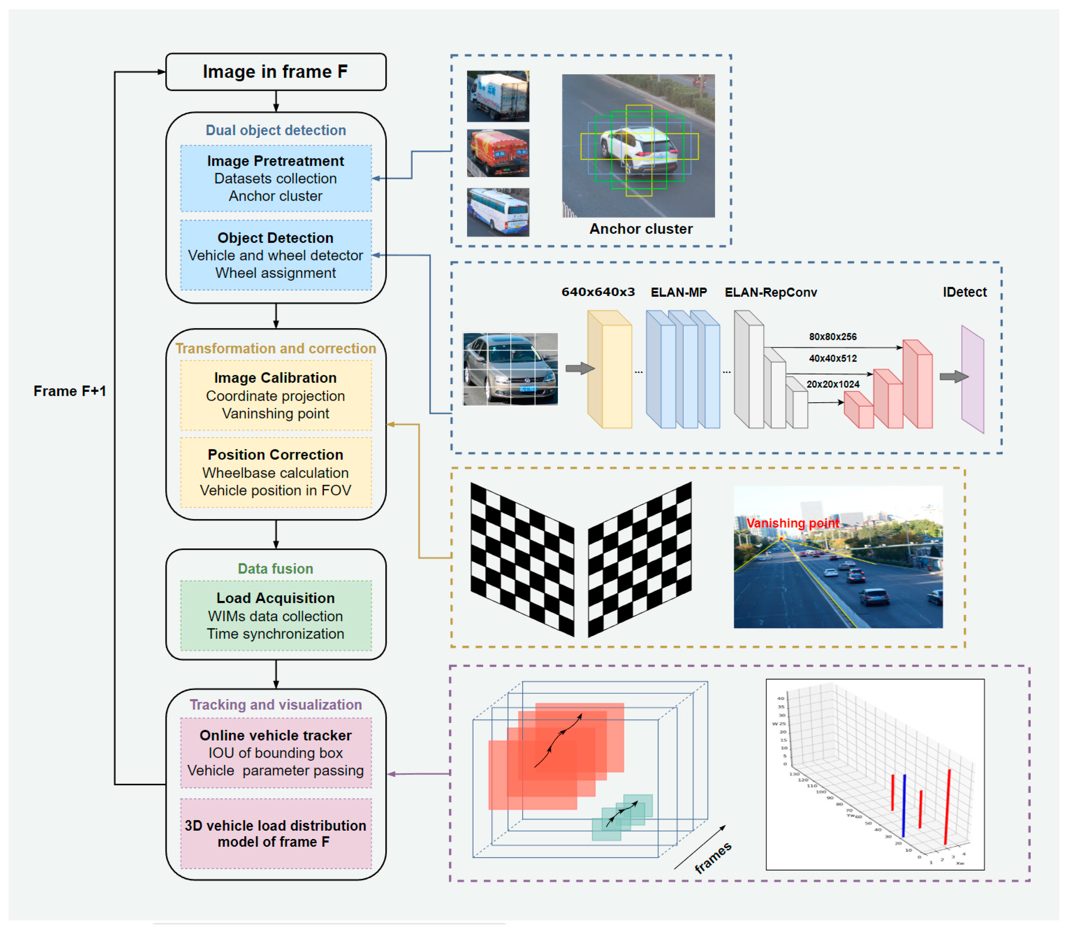
Figure 1 shows a framework of the proposed method for the identification of the spatiotemporal distribution of vehicles on a bridge. The whole process is divided into four stages. Stage 1 is dual-object detection with data pretreatment and a dual-object detector developed with YOLOv7. Data pretreatment prepares the data for detector training and does not involve image processing directly. This step includes adequate data collection and anchor clustering so that the trained detector is able to respond rapidly. As in the image in frame F, all vehicles and wheels in the field of view (FOV) are recognized by YOLOv7, and their center points and the size of the bounding box in the target frame are recorded. After detection, our system separates all objects into a vehicle section and a wheel section. Then, wheels are assigned to their vehicles according to the pixel coordinates of the bounding boxes and center points. Stage 2 is transformation and correction by image calibration. An imaging model and vanishing point theory were selected and merged as a calibration method for accurate coordinate transformation. Because the central points of the vehicles in pictures are floating over the bridge desk, the contact points between the wheels and the ground are chosen to estimate the wheelbase and correct the locations of the vehicles. At the end of stage 2, the vehicle type, wheelbase and corrected position are recorded as vehicle attributes for further calculation. Stage 3 is data fusion between the outputs of the vision detector and WIMs. The original weights of the vehicles are set to zero in the FOV. When vehicles are detected passing through WIMs in the FOV, weight data from Frame F are matched to the vehicle in the corresponding lane by time synchronization. Stage 4 aims to obtain the spatiotemporal spectrum by using a reliable multiobject tracking method. When vehicles are detected in this frame, tracker screens out the same vehicles of this frame before one by one, so that wheelbase and loading information are transmitted in the FOV. These tracking results are plotted as 3D vehicle-loading distributions in Frame F and saved to generate trajectories in the whole FOV.

Figure 1.
Framework of the proposed method.
3. Methodology
3.1. Object Detector Development Based on YOLOv7
Object detection is the basis of identification to calculate the spatiotemporal distributions of vehicle loading on a bridge. YOLOv7 was selected as the object detector in this study. As one of the one-stage object detection algorithms, the YOLO series is simpler in network structure than the two-stage algorithms, as well as faster operation and fewer parameters required. With the explosive growth of monitoring data and the trend towards lightweight sensor devices, YOLOv7 provides the possibility of real-time inference on edge devices and has good computational efficiency. Compared with the previous two versions, which focused on inference speed on GPU, YOLOv7 aims to improve detection speed and accuracy on both GPU and CPU simultaneously. In this project, this algorithm achieves 30FPS real-time inference, which is conducive to enhancing the effectiveness of object tracking in the next stage.
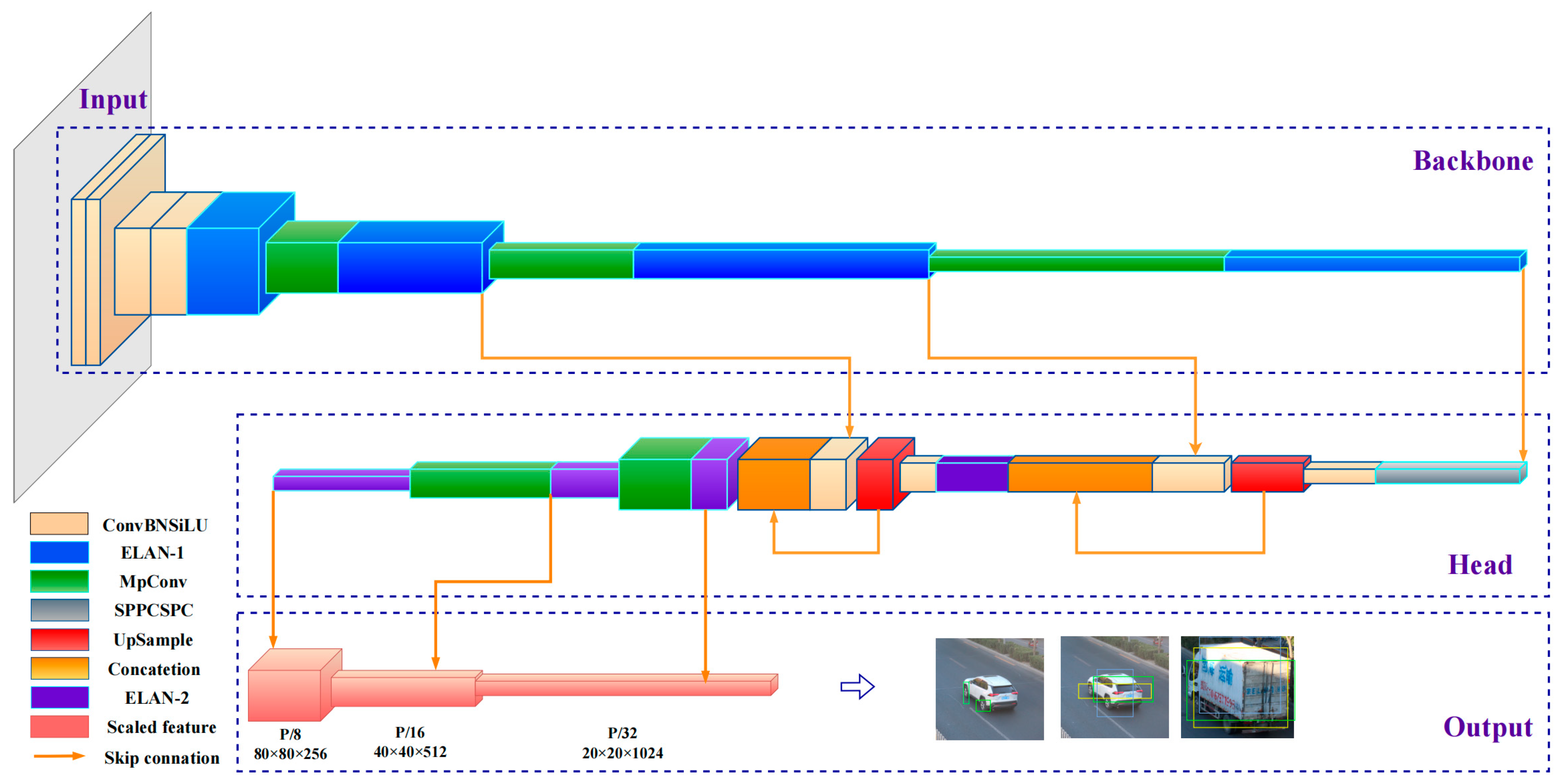
The YOLOv7 algorithm is made up of several key components: input, backbone, head and detection output (as shown in Figure 2). All detected images are scaled to 640 × 640 and input into the backbone network, where scale reduction and deep feature extraction are performed five times. In the head stage, modified PANnet fuses deeper features and then respectively outputs three scaled features at 20 × 20, 40 × 40, and 80 × 80 to comprehensively include objects of different sizes in the prediction.
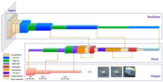
Figure 2.
Architecture of YOLOv7.
In terms of the framework to improve running speed, YOLOv7 uses efficient layer aggregation networks (ELAN), re-parametric convolution (RepConv), and model scaling based on concatenation [34]. The ELAN makes cross-stage connections to combine gradient paths of different lengths so that convolution features at different depths can flow in the partial nonlinear network, which guides deeper layers to converge effectively while gathering more diverse information. The main architecture of an ELAN is given in Table 1. Concatenation-based model scaling adjusts convolutional blocks in width and depth by merging while considering the channel of the block to maintain optimal sampling. In the training process, RepConv divides a whole module into several identical or different module branches; next, computational results from the branches are added based on the additivity of the convolution. In prediction application, these branch modules are integrated into a completely equivalent module, while trained parameters are used for inference, thus achieving multiple model parameter training in one step. The use of different degrees of depth supervision optimize the recall of the algorithm. The total loss of YOLOv7 consists of confidence loss, regression loss and classification loss, and the formula is as follows:
where is the loss gain of three loss portions. The regression positioning loss of all samples is calculated by , which considers three geometric parameters: intersection of union (), center distance and aspect ratio. is calculated as follows:
where is the area intersection ratio between the predicted detection and the ground truth (GT). Here, is the Euclidean distance between the center point of the bounding box and GT and is the diagonal distance that contains the bounding box and the minimum GT. solves the problem of difficulty in backward propagation when is 0. In this context, is the loss parameter of the aspect ratio, considering the similarity of shapes in object matching. In other words, YOLOv7 has improved speed because it renews the network structure and label allocation rule while guaranteeing accuracy.

Table 1.
ELAN structure: The input of the module is the output from the module of input number. A 0 in the input number represents the output of the last layer before ELAN. ELAN-1 and ELAN-2 are the ELAN structures in the backbone and head, respectively. C represents the channel of the module as a pixel filter, which changes with depth in the network.
3.2. Image Calibration Model Applied in Traffic Scene
3.2.1. Calibration Projection
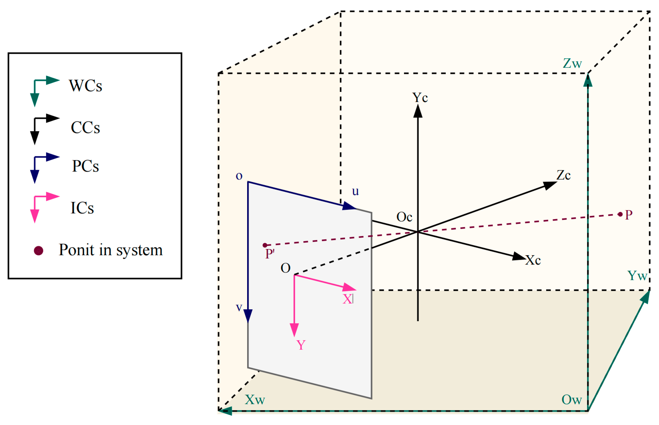
Image calibration is essential for position identification in visual monitoring. The calibration process consists of pinhole imaging inside the camera and external pose estimation, representing the imaging process and position normalization. Figure 3 displays the relationships among the coordinate systems.
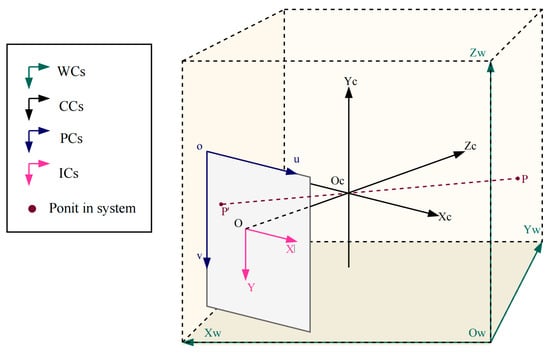
Figure 3.
Calibration geometrical projection. Here, is the world coordinate system (WC); represents the camera coordinate system (CC); is the image coordinate system (IC); and is the pixel coordinate system (PC).
According to the internal coordinate relationship, the optical center of a camera is the origin of , while indicates the offset relative to the parallel pixel coordinates. In the transverse from IC to CC, a pinhole imaging model is revealed based on similar triangles. From CC to WC, a rotation matrix is generated by vectors of the optical axis rotating around three axes of WC and is normalized into an orthogonal unit matrix of order 3 × 3 by Rodrigues’ rotation formula. The translation vector is a third-order column vector of a shift in three directions relative to the origin of . Homogeneous transformation of the whole coordinate system is expressed as follows:
where is the scale ratio from object to optical center; and are the focal lengths by pixel size in X and Y directions; and are the actual offsets of the optical center in PC, which are approximately equal to and ; and are elements of the rotation matrix and translation vector; and represents the projection matrix of the entire transformation process.
As the altitude difference across the monitoring section of the bridge deck is limited, in the world coordinate system is set to 0, so coordinates of any point in the world coordinate system are expressed as . Hence, the projection matrix is simplified as follows:
where is called as the following homography matrix:
Five pairs of reference points are required to solve which has nine unknown variables in the matrix. Under the normalization constraint, is reduced to eight degrees of freedom with at least four reference points needed. The normalization constraint is presented as follows:
3.2.2. Hybrid Calibration Method
There are many studies on image calibration, encompassing methods based on known-size targets, active vision methods and self-calibration methods. Because factor analysis affects calibration results, this study proposes an efficient calibration method that balances the tradeoffs between operability and accuracy.
Zhang’s calibration method is one of the most widely used methods based on two-dimensional targets. With known corner points and position mapping in the chessboard, this traditional calibration technology obtains high precision and convenience in visual research [35]. Due to the invariance of the internal parameter matrix of the camera’s internal structure, this calibration is chosen to estimate the internal parameter matrix because of its accuracy and convenience.
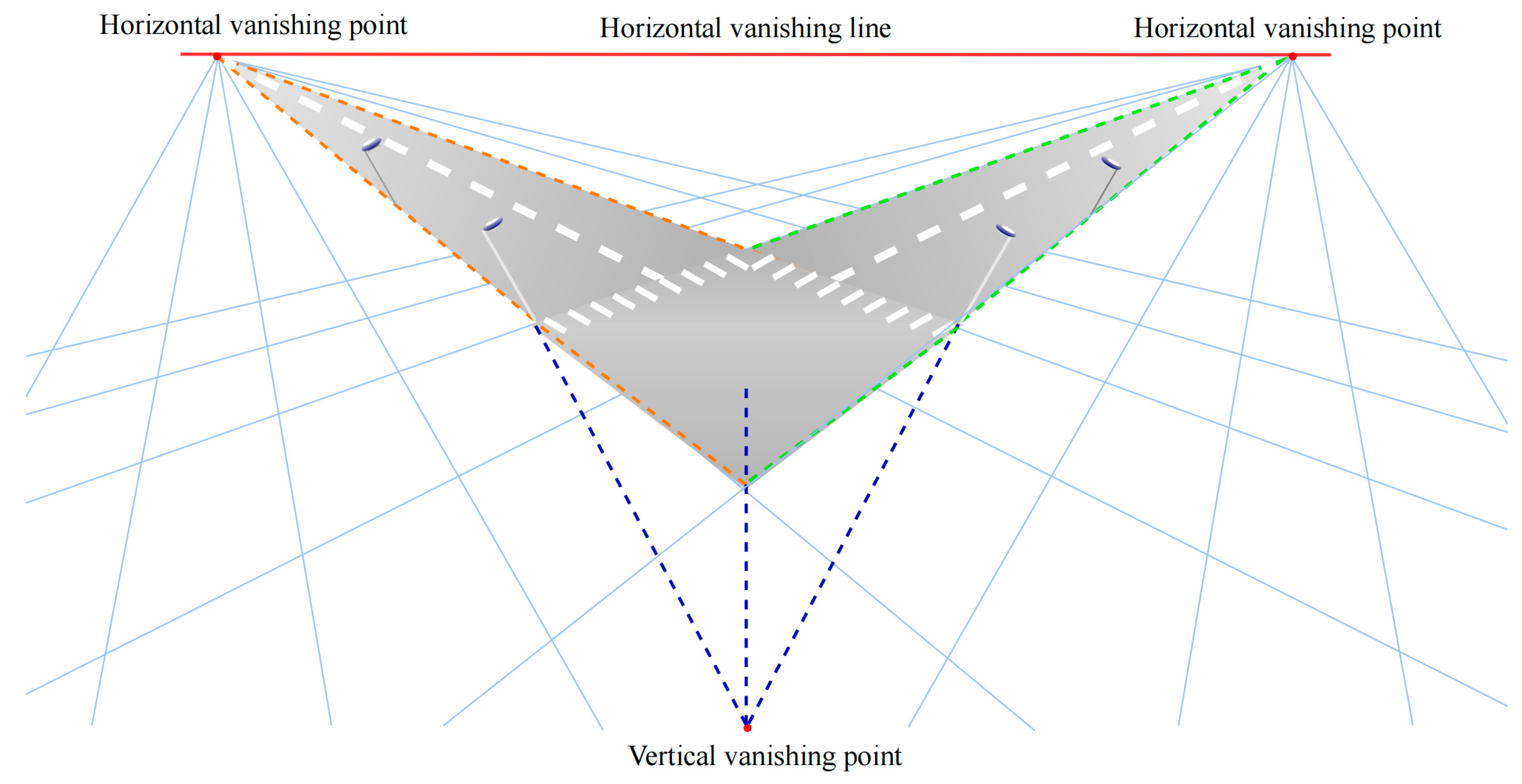
However, the application sites in this study are highways that are larger than the normal field. As a chessboard set in a bridge is obviously smaller than the objects in the FOV, the size mismatch leads to distortion of the angle and distance ratio compared to the actual scene. In order to reduce the impact of the chessboard on the external parameter matrix, vanishing point theory (VP) is imported [36], as shown in Figure 4. These two theories form a new hybrid method, as proposed in this paper.
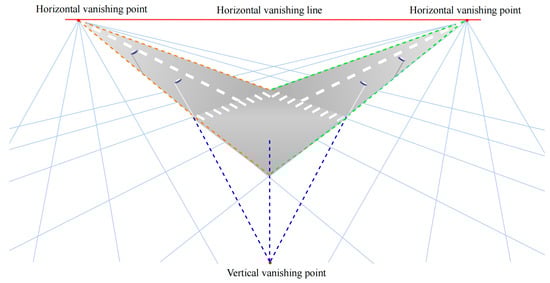
Figure 4.
Vanishing point theory in a traffic scene.
The vanishing point is a focal perspective point formed by parallel lines in a 2D image plane. In a traffic scene picture, the vanishing points of straight roadsides are horizontal vanishing points and form the horizontal vanishing line, which is called the horizon in 3D WC. The outlines of structures perpendicular to roads also focus on one point, the vertical vanishing point. Three vanishing points corresponding to orthogonal groups of parallel lines are used to restore the 3D world. Using traffic marks and ignoring altitude differences on the road, WC in the bridge desk is formed by a pair of orthogonal vanishing points.
Given a known internal reference matrix, the formula of rotation matrix based on the VP is as follows:
where represents any vanishing point chosen. The expression means that a vanishing point in WC is at infinity, and the altitude is set to 0. There is in a unit orthogonal matrix , so the scaling factor is eliminated in the normalization process. With the right-hand rule in graphics, the third vector perpendicular to the horizon is calculated by . The translation vector is solved by another reference point in the image plane:
where reference point is not on the extension line of the vanishing points.
3.3. Multiobject Tracking for Moving Vehicles on Bridges
In this study, MOT requires determination of the correlated metrics of information between the current frame and the previous frames to match new detections to the existing tracks [37]. Inspired by Zhang’s use of Euclidean distance between center points of the detected bounding box [25], this study selects the bounding box as a tracking metric. The IoU tracker does not consider the appearance information of vehicles, nor does it make a prior prediction of known tracks; rather, it only uses a greedy strategy to match bounding boxes of detections one by one. Due to the finite vehicle types and limited changes in the sizes and shapes of bounding boxes in the FOV, adjacent video frames can be used as the main basis for object matching. Moreover, by the actual frame rate of the video stream and the improved detection speed of the YOLOv7 detector, matching can be completed quickly according to the tracking standard.
MOT in this study is based on the assumption that the vehicle detector will detect every track in consecutive frames and that there is a small “gap” in appearance and position between frames. In addition, this object detector has higher accuracy and a higher frame rate, so tracked objects in continuous frames have obvious, high overlap. The method is calculated as follows:
Our tracking method is divided into four main stages: (1) Tracking preparation: A cumulative detection list is formed from all vehicle information collected from the start to the current frame, with analysis of each video frame. This list is sorted based on frame number, and detections with low confidence are filtered by . (2) Track matching: For each tracking target in active track , the maximum matching is executed with all detections in the cumulative detection list corresponding to the current frame. Next, is used to decide whether the best-matched detection can be added to this tracking target. (3) Tracking update: All unmatched detections in the current frame are made candidates for tracking targets, and their motion trajectories are tracked, starting here. (4) Track saving: When tracks in active track list have any historical confidence greater than and the tracking time is not less than , their trajectories are saved in finished track .
In this method, a cumulative detection list is designed to prevent noncontinuous tracking caused by object occlusion and detection abnormality created by the environment and device, which is effective in preventing missed matches. This method does not take advantage of the appearance characteristics of objects; consequently, different objects might continuously match each other if they are detected in adjacent detection frames in a short time. The value of is defined to prevent the false-positive problem of tracking that may be caused by a too-short trajectory. By adjusting its value, the effectiveness of the tracking trajectory can be ensured. The pseudocodes of the main parts of the IoU tracking algorithm are listed in Algorithm 1.
| Algorithm 1 Online dynamic vehicle-tracking algorithm | ||
| Input: video stream, low detection threshold , high detection threshold , threshold , minimum track length in frames . Initialize: active track , finished track . Output: track detection list of frame F . | ||
| 1: | While True do | |
| 2: | Detect video stream before frame F and order list by frame number | |
| 3: | for ; ; do | |
| 4: | if then | |
| 5: | ; | |
| 6: | end if | |
| 7: | if is not null then | |
| 8: | for f = 0 to F; do | |
| 9: | where | |
| 10: | if then | |
| 11: | ||
| 12: | ||
| 13: | ||
| 14: | Remove from | |
| 15: | else if ; then | |
| 16: | Add to | |
| 17: | Remove from | |
| 18: | end if | |
| 19: | for do | |
| 20: | Start new track t with and insert into | |
| 21: | end if | |
| 22: | for do | |
| 23: | if ; then | |
| 24: | Add to | |
| 25: | end if | |
| 26: | for do | |
| 27: | if then | |
| 28: | ||
| 29: | ||
| 30: | end if | |
| 31: | end | |
3.4. Data Fusion
To dynamically obtain the actual weights of vehicles, this study fuses image data from cameras with loading data from WIMs. Vehicle images are a kind of three-dimensional data that require convolution neural networks to complete processing and recognition of pixels. Weight data are generated as sequence form, which are transformed from pressure signals, to electrical signals and then to data signal through the signal-processing module and analogue to the digital (A/D) converter. Due to the difference in data structure between them, this study adopts decision-level data fusion instead of pixel-level fusion and feature-level fusion. That is, to ensure temporal consistency, attribute matching is carried out between an identified vehicle and the transformed vehicle loading to construct a traceable weight distribution and warn of overweight vehicles.
When the axle weight is acquired by the WIMs, the corresponding frame is stamped by time matching and the object coordinates on the image of that frame are transformed to the coordinates on WCs. When a vehicle position condition is met, a weight is assigned to the detection as the vehicle attribute. Considering the matching error of monitoring, the conditions of data fusion are set as follows:
where is the weight value from the WIMs at time . Due to the influence of environmental noise, pressure sensors may respond to non-vehicle objects, so the weight threshold is set to ensure the reliability of the loading data. Here, is the y coordinate of the vehicle in the WCs, while and define the coordinate range of WIMs in the y-direction. Here, is the time when the WIMs obtain the loading and is the time needed to identify vehicles passing through the WIMs in the image. The difference between these times is the matching-time threshold.
4. Case Study
4.1. Preparation of the Detector
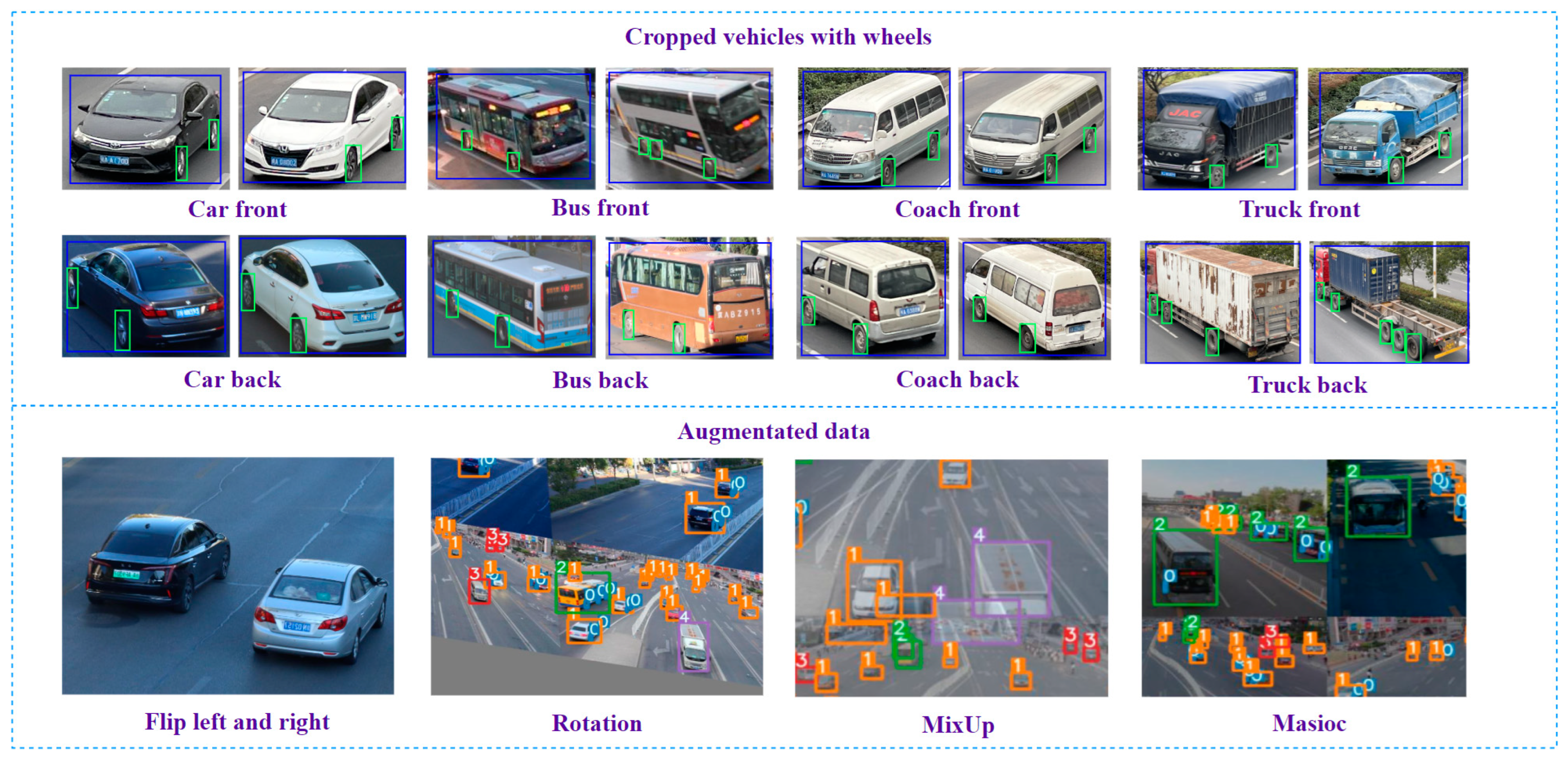
The object detector is trained in CUDA 11.4, CUDNN 11.4, GPU and CPU. According to the purpose of bridge vehicle identification, the authors classified moving objects into four categories: car, bus, coach, and truck. Most pictures in our datasets are frames from a traffic flow video from different perspectives captured by cameras, while the remaining datasets come from ua-detrac as a supplement to prevent overfitting in the training process. In order to reduce the uncertainty associated with changes in environmental conditions, videos are taken of scenes with different vehicle densities, lighting conditions and pitch angles. Apart from normal augmentation methods, such as mirroring, rotation and random cropping, this study also applies Mosaic and MixUp to increase the richness of the image data. Due to the input size of 640 × 640, although most of the pictures are 1920 × 1280, the algorithm is set to fill any picture with fewer than 640 pixels. The dataset proportion for training and validation is 0.7; that is, 2569 pictures are used as the training set and 1101 pictures were used as the validation sets (as shown in Figure 5).
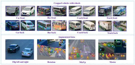
Figure 5.
Datasets preparation.
The training strategies used are summarized as follows: (1) As only detected vehicles and wheels are considered, original anchors are not appropriate for these detection types. Therefore, k-means clustering is used to recalculate anchor groups, and a comparison of the original and updated anchors is presented in Table 2. (2) Wheel recognition is more difficult than vehicle recognition due to their smaller size and lower availability of samples. There is an imbalance between positive examples and negative examples in our training condition. To manage the problem of incomplete training with wheel samples, focal loss is utilized to introduce an attention mechanism in the classification loss function, as follows:
where is the GT label probability of a certain type; is the bounding-box prediction probability; and is the attention mechanism coefficient, which increases the contribution of difficult samples to the loss by increasing the coefficient multiple difference and makes the training model focus on distinguishing difficult features by reducing loss in the training process. (3) To avoid falling into the local optimal solution of gradient descent, this study uses cosine annealing to adjust the learning rate. (4) Because of the limitations of small datasets, transfer learning is adopted to make the model converge quicker. In order to evaluate model performance on multiple targets with imbalanced sample capacity, a PR curve is applied to evaluate the detection accuracy and generalization ability of the model. Figure 6 shows the precision-recall curve (PR curve) for the training results.
Table 2.
Adaptive anchor cluster by k-means of datasets.
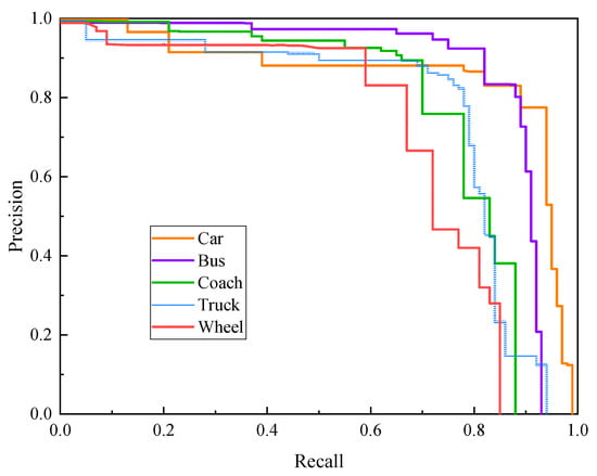
Figure 6.
Precision-recall curve of different objects.
4.2. Verification of Hybrid Calibration Model
A field test is accomplished to verify the advantages of the hybrid method compared to the traditional method using known-size targets for projection matrix resolution. The range of the FOV is a rectangle with a size of 15 × 90, shown as in Figure 7. The authors selected 4 corner points to delimit the rectangle’s scope and 18 internal points in the rectangular area as references. The internal points are the end points of the road marking lines, which are uniformly distributed in the FOV, making calibrations easier and more standard. The origin of the WCs in the FOV is , and the direction from the origin to follows the x-axis, while the direction from the origin to follows the y-axis. According to the right-hand rule, the orientation perpendicular to the bridge desk is the z-axis.

Figure 7.
Reference points of the test in road.
To illustrate the differences, the errors of the two calibration methods in terms of distance and components are compared. Figure 8 plots the comparison of distance errors by a musk heatmap, where the musk threshold is 5.8 m. In the diagram, the same points of the hybrid method are darker in color than those of the traditional method because they are closer to the real points. The maximum value obtained by the traditional method is 5.6 m at Point 9, while the hybrid method found a maximum distance of less than 1 m at Point 7. Among all points, on average, the proposed method reduces the distance error of traditional method by 5 times. The distances in the middle section are larger than those of the edge in the results of both methods. These results clearly demonstrate that distance error mainly appears in the middle of a picture, the result of barrel distortion from the camera lens.
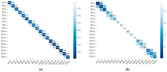
Figure 8.
Comparison of different calibration methods in terms of distances: (a) Point distance of the hybrid method; (b) Point distance of the traditional method.
Component errors of the X and Y coordinates were also analyzed, as shown as in Figure 9. Reference points are divided into three groups, which are presented in lines. Line-1-N represents the X or Y coordinate errors of line-1. N = 1 represents the hybrid method, and N = 2 represents the traditional method. For Method 2, errors in the values of the X coordinates increase with distances in Figure 9a, suggesting that measured reference points deviate from the real points and tend to approach roadsides. At the same time, the trend in the errors of the Y coordinates first shows an increase, then a decrease. The average peak value of the Y errors for Method 2 is about 5 m, close to the value of the distance error. This result suggests that the distance errors are mainly caused by errors in the Y value. By contrast, the errors represented in the three lines corresponding to the results from Method 1 are consistent and stable, and the maximum errors in the values of the X and Y coordinates are lower, a 0.2 m and 1 m; these errors are much lower than those of Method 2.
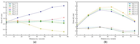
Figure 9.
Comparison of calibration methods in terms of components: (a) Distance errors in the X component; (b) Distance errors in the Y component.
In general, measurement errors are highly relevant to distortion of Y coordinates and value instability of distances from camera position to reference points. These calculated results indicate that the traditional method performs poorly in eliminating error caused by distortion and perspective. The orthogonal VP-based method improves calculation precision, especially in terms of the Y coordinates. It obtains an external reference matrix by perspective and distortion relation of lines, which diminishes the effect of distance errors caused by the camera and has an advantage in terms of the robustness of the data to coordinate transformation. The coordinates of the landing vehicles on the bridge deck are calculated based on the bounding boxes of the vehicles and wheels. Due to non-accumulation of calculation results in the hybrid calibration method, the errors of vehicle coordinates and trajectories are maintained within 1 m, ensuring the accuracy of data on vehicle distribution and trajectory.
4.3. Field Test of the Proposed Method
In the field test, the FOV, including the WIMs is covered by monocular detection, and traffic images are taken continuously. A schematic diagram is shown in Figure 10. To test the feasibility and accuracy of the proposed method for bridge-monitoring applications, the test was carried out on a highway bridge. There are three lanes on this box girder bridge, each of which is 3.75 m wide. Due to a curve in the section of the bridge captured by the camera, this field test ranges from the start of the WIMs to the beginning of the curve, covering a total range of 75 m.
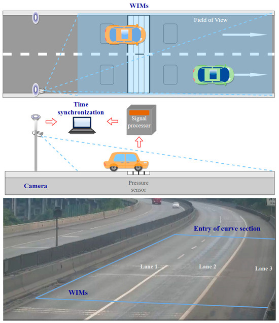
Figure 10.
Data fusion of WIMs and camera.
In order to test the detector effect, the recognition results for objects in the bridge scene were analyzed. Images of 250 frames were selected for each type of vehicle. Accuracy was calculated for four types of vehicle, and recall was tested for the wheels on different vehicles, as shown in Table 3. In terms of vehicle-recognition accuracy, the recognition confidence for vehicles in the coach category was the lowest. Coaches have similar characteristics to cars from some angles, giving rise to slight confusion in identification. However, 94% accuracy is sufficient for the recognition of coaches. Trucks come in various kinds and shapes, which might somewhat limit recognition accuracy, but the accuracy was still 95%. With regard to recall of wheels, the lowest result, 88%, was found for truck, because the number of truck axles spans 2 to 6, which leads to missed detections. At the same time, for some vehicles, at specific angles and greater distances, the pixel area occupied by the wheels is very small, which affects the recall rate. Therefore, in practice, camera placement should cover the FOV and cameras should be angled to capture wheels.
Table 3.
Accuracy of vehicle recognition and recall of wheel recognition.
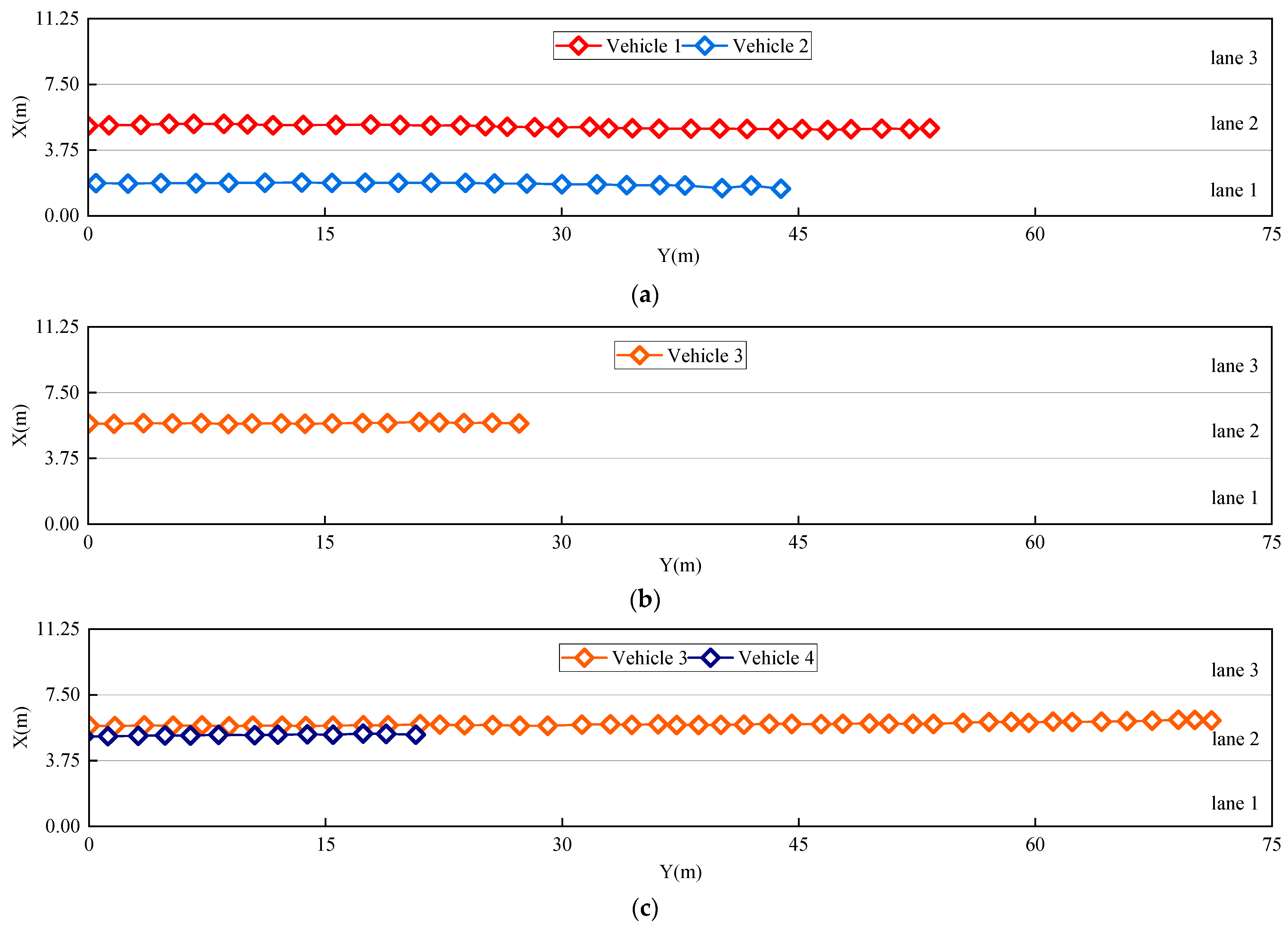
Figure 11 shows the trajectories of the bridge vehicles from the video stream. With our processing algorithm, every five frames, the coordinates obtained are selected as trajectory points to form continuous trajectory maps. The vehicle trajectory is kept in the diagram only while the vehicle is still in the FOV. For example, vehicle 1 and vehicle 2 drive out of the FOV in Figure 11c, so their trajectory information disappears, while vehicle 3 is still in the trajectory from the start frame to the 330th frame. Although positions fluctuate during driving, no vehicles have changed lanes, and vehicles in the same lane maintain similar driving distances, which is consistent with the real conditions in the video. According to relevant regulations, the minimum vehicle length is 3.5 m and the minimum safety distance on the highway is 50 m. Under normal conditions, there are at most two vehicles in each lane in the 75-m-long FOV, as shown in Figure 11c. This method can clearly be used to detect the corresponding vehicle-load distribution.
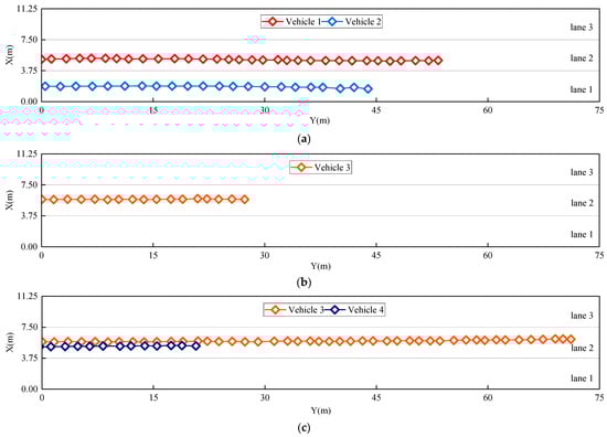
Figure 11.
Dynamic trajectory of vehicles in video stream: (a) shows vehicle trajectories in Frame 120; (b) shows vehicle trajectories in Frame 270; (c) shows vehicle trajectories in Frame 330.
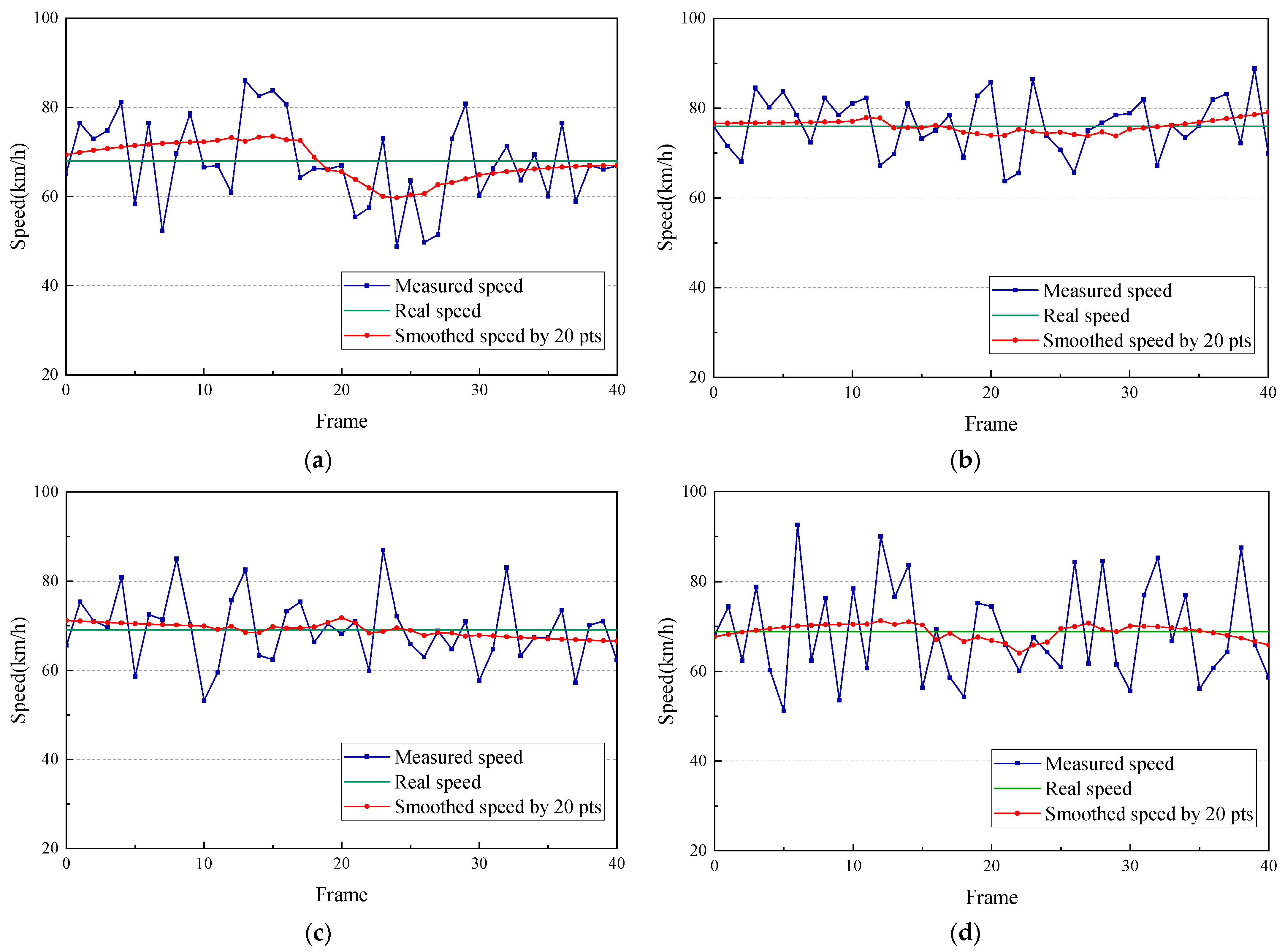
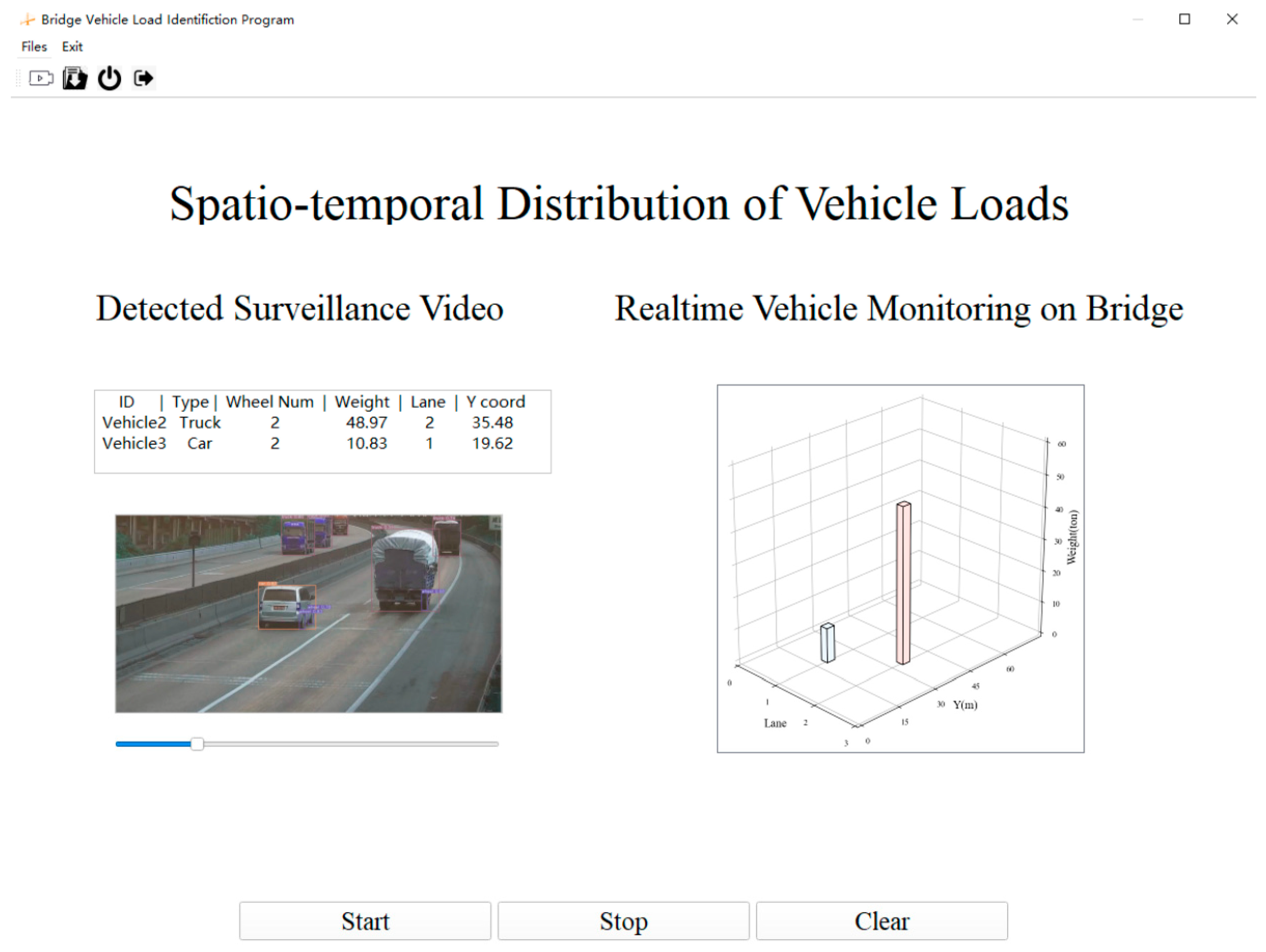
The traffic flows of four vehicles with a duration of 40 frames were selected to calculate real-time measured speed in the images. In Figure 12, the measured speed is smoothed by 20 pts. Smoothed speed represents the average instantaneous speed within 0.67 s, simulating the true speed of the vehicle. The real speed is the instantaneous data measured by the WIMs platform and is based on the assumption of constant speed from the WIMs to the end of the FOV. The sequence diagram of the instantaneous speed shows a wide range of changes over the frames, but the data errors of smoothed speed relative to real speed are only 5.7%, 1.8%, 3.6% and 4.5%, respectively, for four vehicles. Speed through smoothing becomes more stable and closer to the real speed. A car’s speed is displayed in Figure 12b, and the rest of the vehicles are trucks. Figure 12 reveals that the instantaneous speed of this car has a maximum variation of 8%, which is lower than the 34% variation seen for a truck. Thus, the measured values show larger fluctuations and higher frequency of change for larger vehicles. This difference could be interpreted the result of vision bias accumulating frame by frame, as vehicles with a smaller size and a high speed will produce lower calculation errors and more stable speed values. Figure 13 shows one frame of a designed monitoring interface on the bridge, which aims to detect vehicles and wheels while simultaneously providing a 3D distribution of vehicle loading. During video-stream processing, the spatiotemporal distribution of loading is dynamically visualized. A comparison of the traffic conditions on the bridge desk and our measured loading distribution reveals that they are exactly the same. Thus, the algorithm can not only check bridge traffic-flow conditions directly, but it can also provide a chance to research combined loading effects with a digital twin model to elucidate the mechanism by which the bridge responds to deformation and force [38]. It is expected that the refined model of vehicle loading will integrate other loads, combining them into a single bridge load parameter in the BSHM platform. The coupling effect of loading will be represented as simultaneous forces loading on the bridge in the simulation model, which will predict the status of the bridge through deep learning. The main challenge of monitoring loading integration is the unification of time measurement. The data-acquisition intervals and the transmission times of different sensors are not uniform, so it is necessary to align these disparate times when loading the model. At the same time, prediction of bridge states will require considerable training to achieve accurate results. The deformation model will be applied to the digital twin model to predict the future operation and maintenance needs of the bridge in the current environment, which could assist in informed scheduling of bridge maintenance.
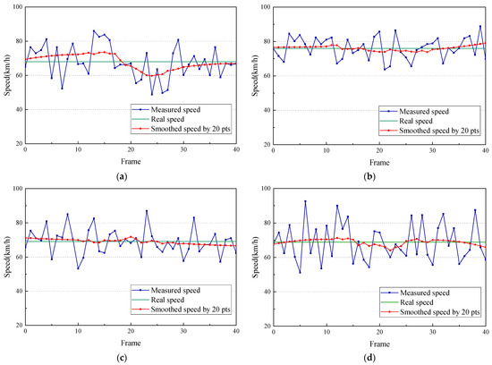
Figure 12.
Speeds of different vehicles from Figure 11: (a) Vehicle1; (b) Vehicle2; (c) Vehicle3; (d) Vehicle4.
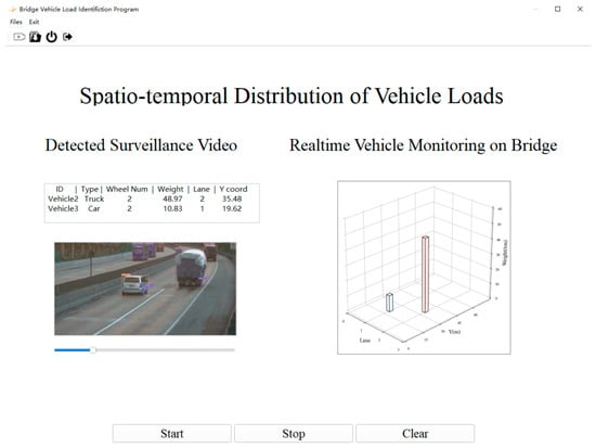
Figure 13.
Real-time vehicle monitoring on a bridge.
5. Conclusions
In this study, a new real-time bridge vehicle-loading-distribution method is proposed. Based on computer vision technology, this method mainly involves dual-object detection, coordinate transformation and correction, data fusion of static weight and position, and vehicle tracking. The main conclusions are as follows:
- A realistic loading distribution is achieved via decision-level data fusion. The detector is trained to support low-decay identification through applicable datasets and strategies. In the field test, the average accuracy of the detector for vehicle types is 96.75%, and the average recall for wheels for different vehicles is 93.25%. This accuracy is sufficient for monitoring dynamic traffic conditions.
- A hybrid coordinate transformation method is proposed that greatly reduces the barrel distortion of the camera lens and the errors caused by perspective. Compared with the traditional method, the proposed method reduces distance error by 5 times on average. Combined with the wheel recognition and the high-precision hybrid transformation method, the wheelbase and coordinates of contact points between the vehicles and the bridge can be calculated.
- A 3D spatiotemporal distribution of vehicles can be visualized in real time following video stream. The trajectory and speed of each vehicle are tracked by an efficient IoU tracker with a rapid response.
However, the following limitations remain: (1) the change in vehicle position is sensitive to the vibration of the bridge deck, which is difficult to eliminate in practice; (2) performance under harsh environmental conditions is one aspect for further improvement. In foggy, rainy, and low-visibility conditions, the edge detection is affected to varying degrees. As there is no processing, this drop in performance will lead to missed and false recognition, affecting the effectiveness of object detection. In addition to enriching datasets by adding more scenes during dataset preparation, as described above, the detector can be improved via image preprocessing section with more images acquired under harsh conditions; and (3) this study only detects vehicles in a limited FOV. In the future, the vehicle-loading distribution of the whole bridge will be studied, and a more accurate and stable method for determining vehicle distribution will be explored to provide instantaneous and multidimensional vehicle-loading data for the BSHM system. Moreover, the integration of this application with other sensors will be explored. Inevitably, it will also be necessary to explore the correlation between spatiotemporal vehicle-load data and acceleration/temperature/displacement to enhance the completeness and support the integration of BSHM.
Author Contributions
Conceptualization, J.Y. and X.M.; methodology, J.Y.; software, J.Y.; validation, J.Y.; formal analysis, J.Y.; investigation, J.Y.; data curation, Z.S. and Y.B.; writing—original draft preparation, J.Y.; writing—review and editing, X.M., Z.S. and Y.B.; visualization, X.M.; supervision, X.M.; project administration, J.Y. and X.M.; funding acquisition, Y.B. and X.M. All authors have read and agreed to the published version of the manuscript.
Funding
This research was funded by the National Natural Science Foundation of China (grant No.52378385) and the Collaborative Innovation Project of Chaoyang District, Beijing (grant No. CYXC2207).
Data Availability Statement
Data available on request due to restrictions eg privacy or ethical. The data presented in this study are available on request from the corresponding author.
Acknowledgments
The first author would like to thank Xudong Jian, Ye Xia and Limin Sun for providing the experimental data of case study gathered from Hebei, China.
Conflicts of Interest
The authors declare no conflicts of interest.
Abbreviations
| SHM | Structural Health Monitoring |
| BSHM | Bridge Structural Health Monitoring |
| WIMs | Weight-in-Motion system |
| BWIMs | Bridge Weight-in-Motion system |
| MFI | Moving Force Identification |
| CA | Cellular Automata |
| Faster R-CNN | Faster Regional-Convolution Neural Network |
| MOT | MultiObject Tracking |
| SORT | Simple Online and Realtime Tracking |
| GVW | Gross Vehicle Weight |
| FOV | Field of View |
| ELAN | Efficient Layer Aggregation Networks |
| RepConv | Re-parametric Convolution |
| GT | Ground Truth |
| IoU | Intersection of Union |
References
- Rizzo, P.; Enshaeian, A. Challenges in bridge health monitoring: A review. Sensors 2021, 21, 4336. [Google Scholar] [CrossRef]
- Sun, Z.; Chen, T.; Meng, X.; Bao, Y.; Hu, L.; Zhao, R. A Critical Review for Trustworthy and Explainable Structural Health Monitoring and Risk Prognosis of Bridges with Human-In-The-Loop. Sustainability 2023, 15, 6389. [Google Scholar] [CrossRef]
- Sujon, M.; Dai, F. Application of weigh-in-motion technologies for pavement and bridge response monitoring: State-of-the-art review. Autom. Constr. 2021, 130, 103844. [Google Scholar] [CrossRef]
- Adresi, M.; Abedi, M.; Dong, W.; Yekrangnia, M. A Review of Different Types of Weigh-In-Motion Sensors: State-of-the-art. Measurement 2023, 225, 114042. [Google Scholar] [CrossRef]
- Burnos, P.; Gajda, J.; Sroka, R.; Wasilewska, M.; Dolega, C. High accuracy Weigh-In-Motion systems for direct enforcement. Sensors 2021, 21, 8046. [Google Scholar] [CrossRef] [PubMed]
- Zhou, H.C.; Li, H.N.; Yang, D.H.; Yi, T.H. Development of moving force identification for simply supported bridges: A comprehensive review and comparison. Int. J. Struct. Stab. Dyn. 2022, 22, 2230003. [Google Scholar] [CrossRef]
- O’Connor, C.; Chan, T.H.T. Dynamic wheel loads from bridge strains. J. Struct. Eng. 1988, 114, 1703–1723. [Google Scholar] [CrossRef]
- Chan, T.H.; Law, S.S.; Yung, T.H.; Yuan, X.R. An interpretive method for moving force identification. J. Sound Vib. 1999, 219, 503–524. [Google Scholar] [CrossRef]
- Law, S.S.; Chan, T.H.; Zeng, Q.H. Moving force identification: A time domain method. J. Sound Vib. 1997, 201, 1–22. [Google Scholar] [CrossRef]
- Law, S.S.; Chan, T.H.; Zeng, Q.H. Moving force identification—A frequency and time domains analysis. J. Dyn. Syst. Meas. Control 1999, 121, 394–401. [Google Scholar] [CrossRef]
- Paul, D.; Roy, K. Application of bridge weigh-in-motion system in bridge health monitoring: A state-of-the-art review. Struct. Health Monit. 2023, 22, 4194–4232. [Google Scholar] [CrossRef]
- O’Brien, E.J.; Jacob, B. European specification on vehicle weigh-in-motion of road vehicles. In Proceedings of the 2nd European Conference on Weigh-in-Motion of Road Vehicles, Lisbon, Portugal, 14–16 September 1998; Office for Official Publications of the European Communities: Luxembourg, 1998; pp. 171–183. [Google Scholar]
- Pimentel, R.; Ribeiro, D.; Matos, L.; Mosleh, A.; Calçada, R. Bridge Weigh-in-Motion system for the identification of train loads using fiber-optic technology. In Structures; Elsevier: Amsterdam, The Netherlands, 2021; Volume 30, pp. 1056–1070. [Google Scholar]
- Yan, W.J.; Hao, T.T.; Yuen, K.V.; Papadimitriou, C. Monitoring gross vehicle weight with a probabilistic and influence line-free bridge weight-in-motion scheme based on a transmissibility-like index. Mech. Syst. Signal Processing 2022, 177, 109133. [Google Scholar] [CrossRef]
- Zona, A. Vision-based vibration monitoring of structures and infrastructures: An overview of recent applications. Infrastructures 2020, 6, 4. [Google Scholar] [CrossRef]
- Khuc, T.; Nguyen, T.A.; Dao, H.; Catbas, F.N. Swaying displacement measurement for structural monitoring using computer vision and an unmanned aerial vehicle. Measurement 2020, 159, 107769. [Google Scholar] [CrossRef]
- Jang, K.; An, Y.K.; Kim, B.; Cho, S. Automated crack evaluation of a high-rise bridge pier using a ring-type climbing robot. Comput.-Aided Civ. Infrastruct. Eng. 2021, 36, 14–29. [Google Scholar] [CrossRef]
- Dong, C.Z.; Catbas, F.N. A review of computer vision–based structural health monitoring at local and global levels. Struct. Health Monit. 2021, 20, 692–743. [Google Scholar] [CrossRef]
- Heidari, A.; Jafari Navimipour, N.; Dag, H.; Unal, M. Deepfake detection using deep learning methods: A systematic and comprehensive review. Wiley Interdiscip. Rev. Data Min. Knowl. Discov. 2023, e1520. [Google Scholar] [CrossRef]
- Jian, X.; Xia, Y.; Sun, S.; Sun, L. Integrating bridge influence surface and computer vision for bridge weigh-in-motion in complicated traffic scenarios. Struct. Control Health Monit. 2022, 29, e3066. [Google Scholar] [CrossRef]
- Chen, Z.; Li, H.; Bao, Y.; Li, N.; Jin, Y. Identification of spatio-temporal distribution of vehicle loads on long-span bridges using computer vision technology. Struct. Control Health Monit. 2016, 23, 517–534. [Google Scholar] [CrossRef]
- Dan, D.; Ge, L.; Yan, X. Identification of moving loads based on the information fusion of weigh-in-motion system and multiple camera machine vision. Measurement 2019, 144, 155–166. [Google Scholar] [CrossRef]
- Maity, M.; Banerjee, S.; Chaudhuri, S.S. (2021, April). Faster r-cnn and yolo based vehicle detection: A survey. In Proceedings of the 2021 5th International Conference on Computing Methodologies and Communication (ICCMC), Erode, India, 8–10 April 2021; pp. 1442–1447. [Google Scholar]
- Jiang, P.; Ergu, D.; Liu, F.; Cai, Y.; Ma, B. A Review of Yolo algorithm developments. Procedia Comput. Sci. 2022, 199, 1066–1073. [Google Scholar] [CrossRef]
- Zhang, B.; Zhou, L.; Zhang, J. A methodology for obtaining spatiotemporal information of the vehicles on bridges based on computer vision. Comput.-Aided Civ. Infrastruct. Eng. 2019, 34, 471–487. [Google Scholar] [CrossRef]
- Kong, X.; Zhang, J.; Wang, T.; Deng, L.; Cai, C.S. Non-contact vehicle weighing method based on tire-road contact model and computer vision techniques. Mech. Syst. Signal Process. 2022, 174, 109093. [Google Scholar] [CrossRef]
- Feng, M.Q.; Leung, R.Y.; Eckersley, C.M. Non-contact vehicle weigh-in-motion using computer vision. Measurement 2020, 153, 107415. [Google Scholar] [CrossRef]
- Zhu, J.; Li, X.; Zhang, C. Fine-grained identification of vehicle loads on bridges based on computer vision. J. Civ. Struct. Health Monit. 2022, 12, 427–446. [Google Scholar] [CrossRef]
- Gan, Y.; Wang, P.; Han, W.; Chen, S.; Zhang, S.; Yuan, Y. Automatic generation of fine-grained traffic load spectrum via fusion of weigh-in-motion and vehicle spatial–temporal information. Comput.-Aided Civ. Infrastruct. Eng. 2022, 37, 485–499. [Google Scholar]
- Zhu, J.; Li, X.; Zhang, C.; Shi, T. An accurate approach for obtaining spatiotemporal information of vehicle loads on bridges based on 3D bounding box reconstruction with computer vision. Measurement 2021, 181, 109657. [Google Scholar] [CrossRef]
- Ge, L.; Dan, D.; Li, H. An accurate and robust monitoring method of full-bridge traffic load distribution based on YOLO-v3 machine vision. Struct. Control Health Monit. 2020, 27, e2636. [Google Scholar] [CrossRef]
- Kapania, S.; Saini, D.; Goyal, S.; Thakur, N.; Jain, R.; Nagrath, P. Multi object tracking with UAVs using deep SORT and YOLOv3 RetinaNet detection framework. In Proceedings of the 1st ACM Workshop on Autonomous and Intelligent Mobile Systems, Bangalore, India, 10 January 2020; pp. 1–6. [Google Scholar]
- Hou, X.; Wang, Y.; Chau, L.P. Vehicle tracking using deep sort with low confidence track filtering. In Proceedings of the 2019 16th IEEE International Conference on Advanced Video and Signal Based Surveillance (AVSS), Taipei, Taiwan, 18–21 September 2019; IEEE: New York, NY, USA; pp. 1–6. [Google Scholar]
- Wang, C.Y.; Bochkovskiy, A.; Liao, H.Y.M. YOLOv7: Trainable bag-of-freebies sets new state-of-the-art for real-time object detectors. In Proceedings of the IEEE/CVF Conference on Computer Vision and Pattern Recognition, Vancouver, BC, Canada, 20–22 June 2023; pp. 7464–7475. [Google Scholar]
- Zhang, Z. A flexible new technique for camera calibration. IEEE Trans. Pattern Anal. Mach. Intell. 2000, 22, 1330–1334. [Google Scholar] [CrossRef]
- Kong, H.; Audibert, J.Y.; Ponce, J. Vanishing point detection for road detection. In Proceedings of the 2009 IEEE Conference on Computer Vision and Pattern Recognition, Miami, FL, USA, 20–25 June 2009; IEEE: New York, NY, USA; pp. 96–103. [Google Scholar]
- Bochinski, E.; Eiselein, V.; Sikora, T. High-speed tracking-by-detection without using image information. In Proceedings of the 2017 14th IEEE International Conference on Advanced Video and Signal Based Surveillance (AVSS), Lecce, Italy, 29 August–1 September 2017; IEEE: New York, NY, USA; pp. 1–6. [Google Scholar]
- Meng, X.; Xiang, Z.; Xie, Y.; Ye, G.; Psimoulis, P.; Wang, Q.; Yang, M.; Yang, Y.; Ge, Y.; Wang, S.; et al. A discussion on the uses of smart sensory network, cloud-computing, digital twin and artificial intelligence for the monitoring of long-span bridges. In Proceedings of the 5th Joint International Symposium on Deformation Monitoring (JISDM 2022), Valencia, Spain, 20–22 June 2023. [Google Scholar]

Disclaimer/Publisher’s Note: The statements, opinions and data contained in all publications are solely those of the individual author(s) and contributor(s) and not of MDPI and/or the editor(s). MDPI and/or the editor(s) disclaim responsibility for any injury to people or property resulting from any ideas, methods, instructions or products referred to in the content. |
© 2024 by the authors. Licensee MDPI, Basel, Switzerland. This article is an open access article distributed under the terms and conditions of the Creative Commons Attribution (CC BY) license (https://creativecommons.org/licenses/by/4.0/).