Abstract
Solar photovoltaic energy generation has garnered substantial interest owing to its inherent advantages, such as zero pollution, flexibility, sustainability, and high reliability. Ensuring the efficient functioning of PV power facilities hinges on precise fault detection. This not only bolsters their reliability and safety but also optimizes profits and avoids costly maintenance. However, the detection and classification of faults on the Direct Current (DC) side of the PV system using common protection devices present significant challenges. This research delves into the exploration and analysis of complex faults within photovoltaic (PV) arrays, particularly those exhibiting similar I-V curves, a significant challenge in PV fault diagnosis not adequately addressed in previous research. This paper explores the design and implementation of Support Vector Machines (SVMs) and Extreme Gradient Boosting (XGBoost), focusing on their capacity to effectively discern various fault states in small PV arrays. The research broadens its focus to incorporate the use of optimization algorithms, specifically the Bees Algorithm (BA) and Particle Swarm Optimization (PSO), with the goal of improving the performance of basic SVM and XGBoost classifiers. The optimization process involves refining the hyperparameters of the Machine Learning models to achieve superior accuracy in fault classification. The findings put forth a persuasive case for the Bees Algorithm’s resilience and efficiency. When employed to optimize SVM and XGBoost classifiers for the detection of complex faults in PV arrays, the Bees Algorithm showcased remarkable accuracy. In contrast, classifiers fine-tuned with the PSO algorithm exhibited comparatively lower performances. The findings underscore the Bees Algorithm’s potential to enhance the accuracy of classifiers in the context of fault detection in photovoltaic systems.
1. Introduction
Solar PV generation has risen as a significant player in the renewable energy sector due to its numerous advantages, which include no emissions, sustainability, adaptability, and dependable performance [1]. As the installed capacity of PV systems continues to expand globally, the urgency to ensure their smooth operation also increases. Among the utmost operational concerns is the effective detection and management of faults in these systems. Fault detection is a vital measure that not only protects the reliability and safety of PV power plants but also aids in maximizing profitability and circumventing costly maintenance. Despite the obvious need for efficient fault detection, the process is fraught with challenges, especially on the Direct Current (DC) side of PV systems. Conventional protection devices often fail when it comes to accurately detecting and classifying faults, creating a significant gap in the overall management and protection of PV systems [2,3]. Nevertheless, it is important to note that the current guidelines for protecting PV systems only cover the AC side and are unable to detect and identify faults on the DC side. Fault analysis in solar PV arrays is crucial to averting any adverse or hazardous conditions resulting from faults within the array. Quick fault detection and timely resolution in solar PV arrays are essential. Inefficient fault detection can result in power loss, heightened fire risks, and other safety concerns [4,5]. Different types of failures can arise in photovoltaic systems. Therefore, understanding the failures observed in practical settings is crucial before establishing monitoring and fault identification methods. This task mainly involves classifying each kind of electrical fault that might occur in PV arrays. Therefore, researchers have been working on developing Machine Learning (ML) methods that can detect faults accurately and reliably. ML algorithms can learn the relationships between the input and output parameters of a PV system without relying on a pre-defined equation. The most common approach to detecting faults in a PV system is to analyze its electrical output, including the current, voltage, and power, if this information is available through monitoring [6]. The obtained data are then compared to that of a reference system. Trained models can be employed for fault detection by utilizing previous data from when the system was known to be functioning properly. If a fault occurs, the system’s behavior will deviate from that described by the trained model, indicating the presence of a fault.
ML methods offer several advantages over other artificial intelligence (AI) and threshold-based techniques, including being data-driven, scalable, automated, capable of continuous learning, and having high predictive accuracy. In the field of PV systems, various ML algorithms have been employed. For instance, researchers have developed probabilistic neural network schemes (PNN) based on manufacturers’ datasheets for health monitoring of the DC side of photovoltaic array [7]. In another study [8], Random Forest (RF) learning was employed as an ensemble method for fault diagnosis in PV arrays. The methodology utilized array voltage and string currents for the diagnostic process. Conventional neural networks (CNNs) and electrical time series graphs were used to develop a fault detection model for PV systems [9]. In [10], a kernel-based extreme learning machine (KELM) was proposed for detecting a wide range of faults in PV systems, which demonstrated promising results using seven inputs and five outputs. In [11], a cloud-based monitoring system was introduced, leveraging the Support Vector Machine (SVM) for fault detection. A binary SVM classifier was presented in [12], which was able to identify abnormalities in the output DC and power using a PSIM simulation of a grid-connected PVS. In [13], a SVM was utilized along with four years of practical data to identify and categorize faults in strings and inverters. In reference [14], Random Under-Sampling Boosting (RUSBoost) was employed to identify different types of faults occurring on the DC side of the photovoltaic system. Traveling-Wave (TW) and Machine Learning (ML) based on RF classification, serving as a faster alternative to over-current protection, were employed, as detailed in reference [15]. The author of [16] proposed the use of XGBoost for fault detection and diagnosis in photovoltaic arrays. The algorithm is based on feature parameters such as irradiance, temperature, current, and power. The experimental results demonstrate that this method outperforms other Machine Learning techniques in achieving accurate fault diagnosis for photovoltaic arrays. Nevertheless, these fault detection models come with their own set of challenges. They often require a large dataset for training, tend to show reduced accuracy when detecting faults with low-percentage mismatches or high impedance, and can be somewhat unreliable since they often rely on a single classifier. Additionally, many of these methods do not offer a comparative approach to selecting the best classifier, and most cannot identify the specific type of fault or determine its severity [17].
For fault detection in PV arrays, hybrid methods combine multiple algorithms, balancing their strengths and weaknesses for improved results. These methods provide flexibility for addressing diverse data patterns in PV arrays, even when faced with anomalies or non-uniform PV systems. Additionally, hybrid methods counteract issues such as noise and overfitting, ensuring the models remain effective in real-world scenarios, rather than just on training data. Numerous studies and applications have showcased the effectiveness of hybrid methods in PV fault detection. For example, in [18], CART, KNN, and RF are introduced, incorporating Data Dimensionality Reduction Strategy (DDRS) and Principal Component Analysis (PCA) for feature extraction and dimensionality reduction. The aim is to identify various fault scenarios in photovoltaic systems, including PV array faults, arc faults, line-to-line faults, open-circuit faults, shading issues, and MPPT unit failures. In [19], the model utilizes I-V characteristics to concentrate on line-to-line (LL) faults at varying mismatch and impedance levels. The research employed a probabilistic ensemble learning model, integrating a Support Vector Machine (SVM), Naive Bayes (NB), and k-Nearest Neighbors (KNN). In [20], the researchers introduced a Shifted Windows (Swin) Transformer optimized by Particle Swarm Optimization (PSO), which is utilized for the detection of various types of photovoltaic (PV) faults, including the line-to-line fault and open-circuit fault, as well as partial shading. Combining PSO with Artificial Neural Networks (ANNs) creates a system that combines the global search capability of PSO with the precision and adaptability of neural networks [21]. While the PSO algorithm has the advantage of requiring fewer input parameters and being easily adjustable, it is prone to becoming trapped in local optima, potentially missing the global optimal approximate solution or not thoroughly addressing certain intricate fault scenarios. Similarly, integrating the Genetic Algorithm (GA) with ANNs offers a powerful and flexible solution for fault detection in photovoltaic arrays, as discussed in [22]. While this approach has shown promise in enhancing fault detection accuracy, it may bring about complexity, potentially resulting in prolonged training durations and increased computational demands, especially when not optimized efficiently. Ref. [23] proposed three potent Machine Learning (ML) algorithms for diagnosing various faults in photovoltaic (PV) arrays, which are Categorical Boosting (CatBoost), Light Gradient Boosting Method (LGBM), and Extreme Gradient Boosting (XGBoost). Ref. [24] employed both threshold methods and Machine Learning (ML) techniques to detect and categorize various faults, including SC, OC, shadow effects, and bypass diode faults, by analyzing attributes such as the current, voltage, and peaks from the I-V characteristics. They contrasted Multi-Layer Perceptron (MLP) with Radial Basis Function (RBF) and executed the strategy on a Field Programmable Gate Array (FPGA). Nonetheless, their approach was based on simulated data and the threshold method, potentially making it highly dependent on system parameters and the precision of threshold limits. In response to the previously discussed challenges, this study presents a reliable line-to-line (LL) and open-circuit (OC) fault detection technique for PV arrays. The primary findings and contributions of the research study presented in this paper can be outlined as:
- The exploration and analysis of complex faults within PV arrays. A small-scale PV system was built to enhance the accuracy of Machine Learning classifiers for PV systems. This system, designed to replicate real-world solar complexities, simulated actual challenges by introducing specific faults. The goal was to produce a high-quality, realistic dataset for training Machine Learning algorithms, ensuring they are well prepared for genuine applications.
- The application of Machine Learning methods, notably Support Vector Machines (SVMs) and Extreme Gradient Boosting (XGBoost), has been employed. These methodologies have exhibited considerable efficacy in detecting various fault conditions in PV arrays.
- Optimization algorithms, specifically the Bees Algorithm (BA) and Particle Swarm Optimization (PSO), have been employed to enhance the performance of SVM and XGBoost classifiers. The optimization process primarily focuses on tuning the hyperparameters of these models to maximize the accuracy in fault classification, providing a holistic approach to PV fault detection and management.
A novel fault detection FD-SVM and XGBoost setups have been proposed and tested to discriminate LL and OC faults by optimizing their parameters using optimization algorithms. Notably, these setups require only three samples to effectively determine the nature and behavior of the faults.
2. A Small-Scale PV Array
A small-scale PV array typically consists of a limited number of PV panels arranged to convert sunlight into electricity. This setup is ideal for laboratory testing due to its compact size and manageability. Their small-scale nature allows for easy fault introduction and monitoring, ensuring accurate results without the complexities of large-scale systems.
2.1. Experimental Setup
A small-scale PV array was constructed using Polycrystalline Mini Solar Cell Panel Module DIY to validate the performance of the proposed approach on PV systems. The array consisted of five parallel-connected strings, with each string comprising twenty modules in series. Detailed specifications of the PV modules can be found in Table 1. To determine the I-V curve for a PV array, the current supplied between zero current and the short-circuit current must be gauged. The voltage and current outputs from the PV array were captured using the Pasan solar sun simulator, in collaboration with the Loughborough University laboratory, as illustrated in Figure 1.

Table 1.
Parameters of main components in Polycrystalline Mini Solar Panel Module DIY PV system under standard test conditions (STCs).
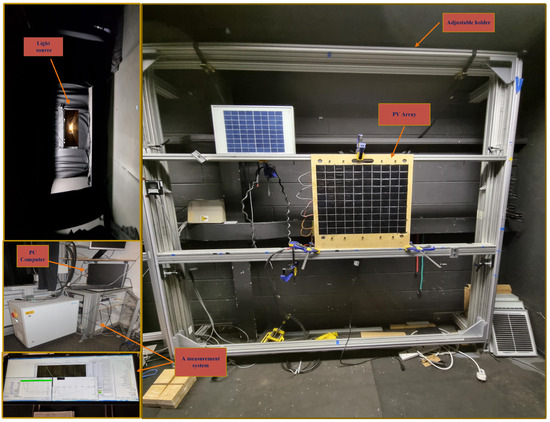
Figure 1.
Experimental setup of PV array with measuring devices.
The Pasan sun simulator, developed by the Pasan Engineering Company, is a dedicated device designed to mimic solar irradiance, testing photovoltaic (PV) cells and modules [25]. It facilitates the capture of current–voltage (I-V) characteristic curves of PV devices in controlled and repeatable conditions. This allows researchers and manufacturers to evaluate the efficacy of their devices and refine their designs. Commonly, the Pasan sun simulator consists of a light source, a collimating lens, and a filter system to create a spectrum that closely matches natural sunlight. The device also includes an adjustable holder to accommodate the PV device being tested, as well as a measurement system for capturing the I-V curves. By replicating controlled solar irradiance conditions, the Pasan sun simulator facilitates precise measurements for research and manufacturing objectives.
2.2. Validating the Model for PV Modules
In this experimental study, a dataset encompassing both normal and faulty scenarios was recorded. The faulty cases included: F1 and F2 (intra-string line-to-line faulst) with large and small voltage differences, respectively; F3 (cross-string line-to-line fault); and F4 (open-circuit fault) affected by the line-to-line (LL) and open-circuit (OC) faults. Therefore, a total of data samples were recorded for each case, representing both faulty and healthy conditions, under standard test conditions (STCs) with a temperature level of 25 °C and an irradiance level of 1000 W/m2. The I-V curve for the entire PV array was tested five times for each case. The goal was to produce a high-quality, realistic dataset for training Machine Learning algorithms, ensuring they are well prepared for real applications.
2.3. Typical Faults Curves and Interpretation
Photovoltaic (PV) power production systems have different types of faults, similar to other types of power plants in terms of fault sensitivity. Nonetheless, there are several potential benefits to using PV systems. Firstly, PV modules are constrained by voltage and current, and their performance is notably influenced by temperature and insulation. Moreover, PV panels operate at a and closely approaching 80%, at which point Maximum Power Point Tracking is utilized [26]. Any DC-side fault that arises poses particular issues, as low fault currents make these faults difficult to detect and diagnose. The ability to accurately evaluate faults requires an understanding of the causes and types of faults to support dealing with these problems and reduction in harms.
2.3.1. Line-to-Line Fault in a PV Array under STC
Line-to-line faults () occur when a low-resistance connection unintentionally links two points within an electrical network system that have different potentials. In the context of PV systems, typically encompass short-circuit faults either between PV modules or among cables of arrays that have differing potentials. Within an array, can occur due to cable insulation failures, accidental current-carrying conductor short circuits, and poor insulation separating string connectors. The current study makes the assumption that there is no ground point involvement in the . This is because where have a ground point, they can be classified as ground faults. This study investigates three classes of at varying locations:
- (a)
- Intra-string LL fault with large voltage difference
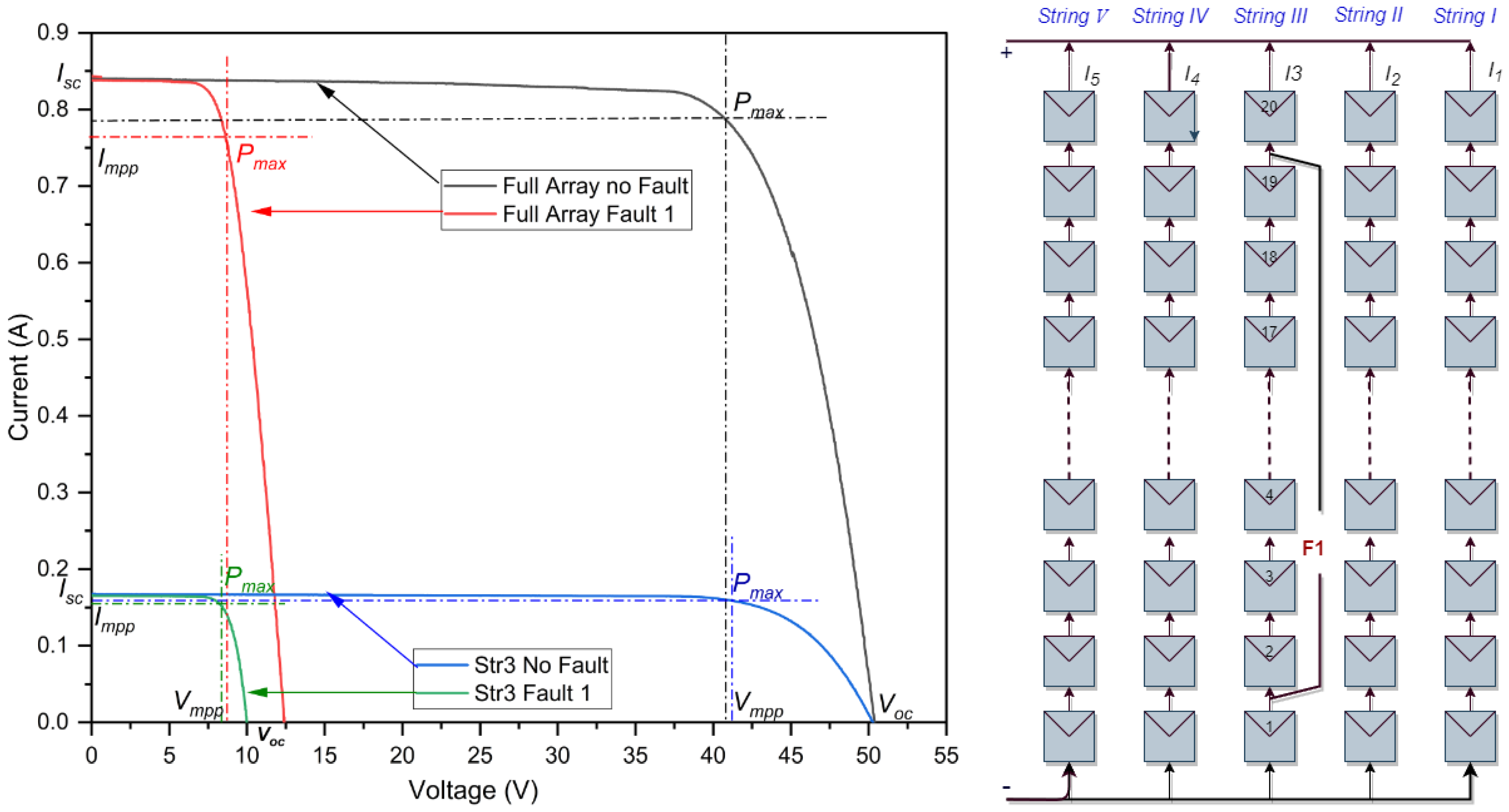
The intra-string short-circuit fault illustrated in Figure 2 is characterized as a line-to-line fault (LLF) with a significant voltage difference and variation across 18 modules. The results obtained from actual experimental measurements, as detailed in Table 2, provide a clear understanding of the consequences of a line-to-line fault featuring a substantial voltage discrepancy. In an optimally functioning or ‘healthy’ state, the system displays an efficiency rate of 20.07%. This healthy state records a of 51.25 V and an of approximately 0.8414 A. However, upon the introduction of a fault, the system’s efficiency drops dramatically to 4.13%. This drastic drop in efficiency is reflected by the sharp drop in voltage, as the contracts sharply from the initial 51.25 V down to a mere 13.88 V . Nonetheless, the current appears to be fairly stable, experiencing only a slight deviation around as a result of the low-resistance path. The cumulative efficiency loss ratio due to this fault is 15.94%, which confirms the seriousness of the impact that such a fault can have on the overall operational efficiency of the PV system. However, the impact of this fault on string 3 is illustrated by the blue and green curve in Figure 2. This decrease is evident in the sharp decline in the voltage, dropping from the initial 51.2879 V to a mere 11.5332 V . This underscores the crucial nature of timely fault detection and rectification to maintain optimal performance levels in photovoltaic systems.
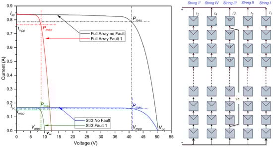
Figure 2.
I-V curves of the PV array in a line-to-line fault with a large voltage difference.
Table 2.
Simulation outcomes of a line-to-line fault with large voltage difference.
- (b)
- Intra-string LL fault with small voltage difference
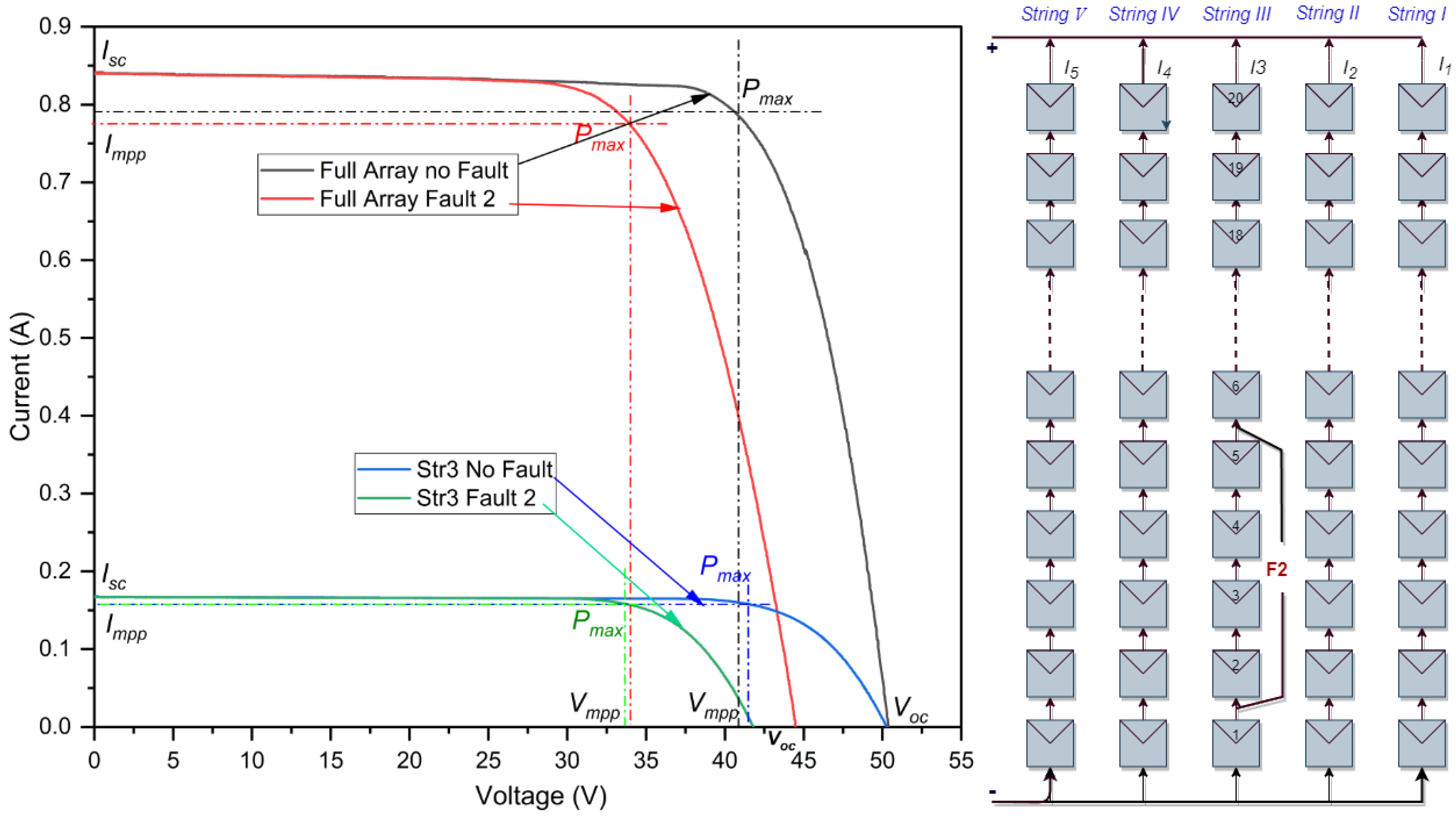
In the graphical representation shown in Figure 3, a short-circuit fault is observed within the third string. This particular fault is defined as an with a small difference in voltage and variation spanning four modules. Referring to the data summarized in Table 3, the most striking feature of this fault is the stability of the current value , despite the noticeable drop in voltage. When the fault appears, the current remains constant at 0.84 A , whereas the voltage notably drops from 51.25 V to 47.30 V . In its optimal state, the system operates at 20.07% efficiency. However, in the presence of the fault, the efficiency drops slightly to 16.46%. This change indicates a loss rate of 3.61%, highlighting the profound impact that these faults have on the overall system performance. However, the impact of this fault on string 3 is illustrated by the blue and green curve in Figure 3. The reduction is evident in the slight decline in the voltage, dropping from the initial 51.2879 V to just 47.6768 V , resulting in a power loss of 18.5997% in string 3.
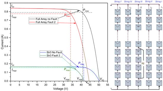
Figure 3.
I-V curves of the PV array in a line-to-line fault with small voltage difference.
Table 3.
Simulation outcomes of a line-to-line fault with small voltage difference at STC.
- (c)
- Cross-string LL fault
As depicted in Figure 4, the simulation reveals the fourth short-circuit fault, which occurs between the third and fourth strings. This LLF has a 10-module level difference between the two strings. The findings of the simulation results are given in Table 4. In the case of a health system, the efficiency reaches 20.07%. However, after the fault occurs, there is a slight decrease in efficiency to 19.80%. This difference, although small at 0.27%, can be significant in a real-world context. Nevertheless, the effect of this fault on string 3 is depicted by the blue and green curve shown in Figure 4. This decline is observable in the slight reduction in power, falling from the initial 13.0882 w to just 12.8421 w , leading to a power loss of 01.8803% in string 3. Since this fault does not induce a dramatic shift in the system’s operational metrics, it underscores the challenge of identifying such faults. This subtlety can jeopardize the system’s reliability and efficiency, as faults of this nature can persist undetected, causing latent damage or degradation over time.
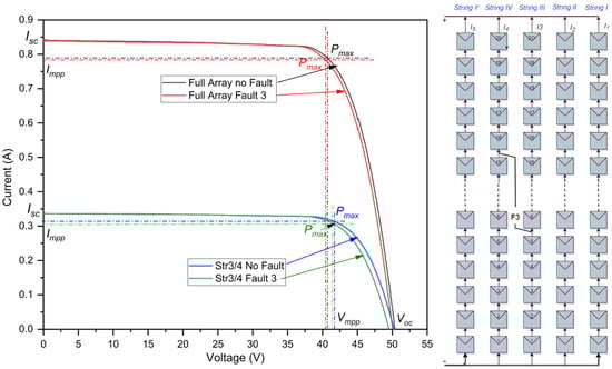
Figure 4.
I-V curves of the PV array in cross-string line-to-line fault.
Table 4.
Simulation outcomes of a cross-string line-to-line fault at STCs.
2.3.2. Open-Circuit Fault under STC
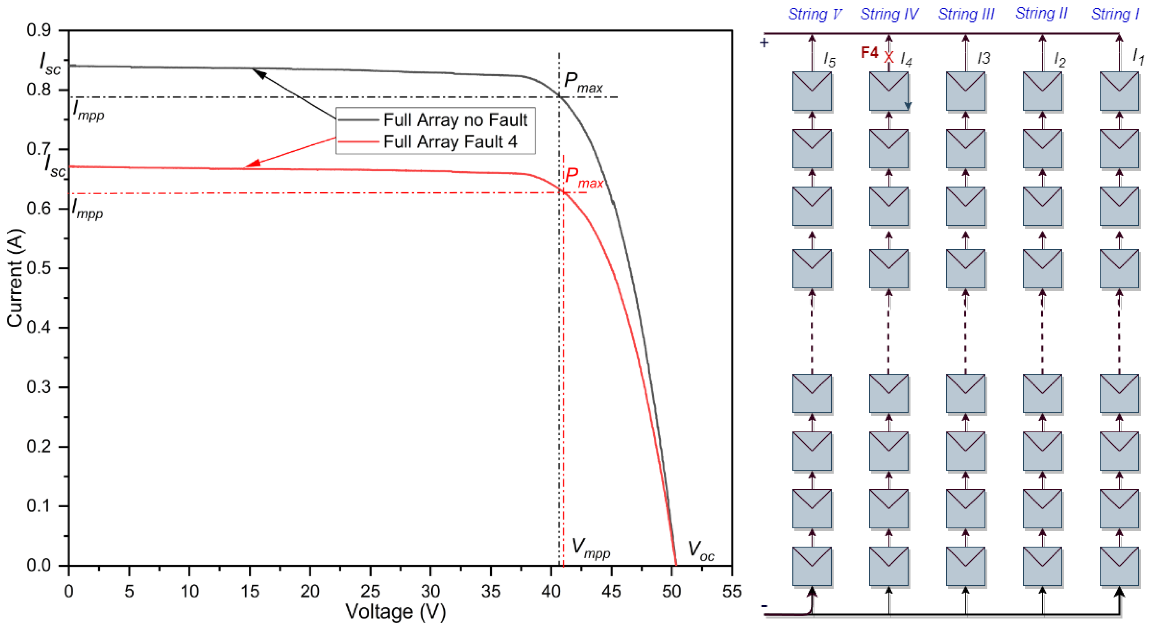
Figure 5 illustrates the open-circuit fault that took place in the fourth string of the PV array. The I-V characteristics of this faulty array are compared with those of a non-faulty array under normal operating conditions. The results of this simulation are detailed in Table 5 and visualized in Figure 5. It becomes clear that the open-circuit fault does not generate a substantial fault current. In the event of this fault, due to one out of five strings being disconnected, significant power losses occur, amounting to approximately 20% of the rated power. While the open voltage remains largely consistent, there is a linear decline in the maximum power and short-circuit current proportional to the number of disconnected strings.
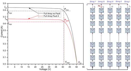
Figure 5.
I-V curves of the PV array during open-circuit fault.
Table 5.
Simulation outcomes of an open-circuit fault at STCs.
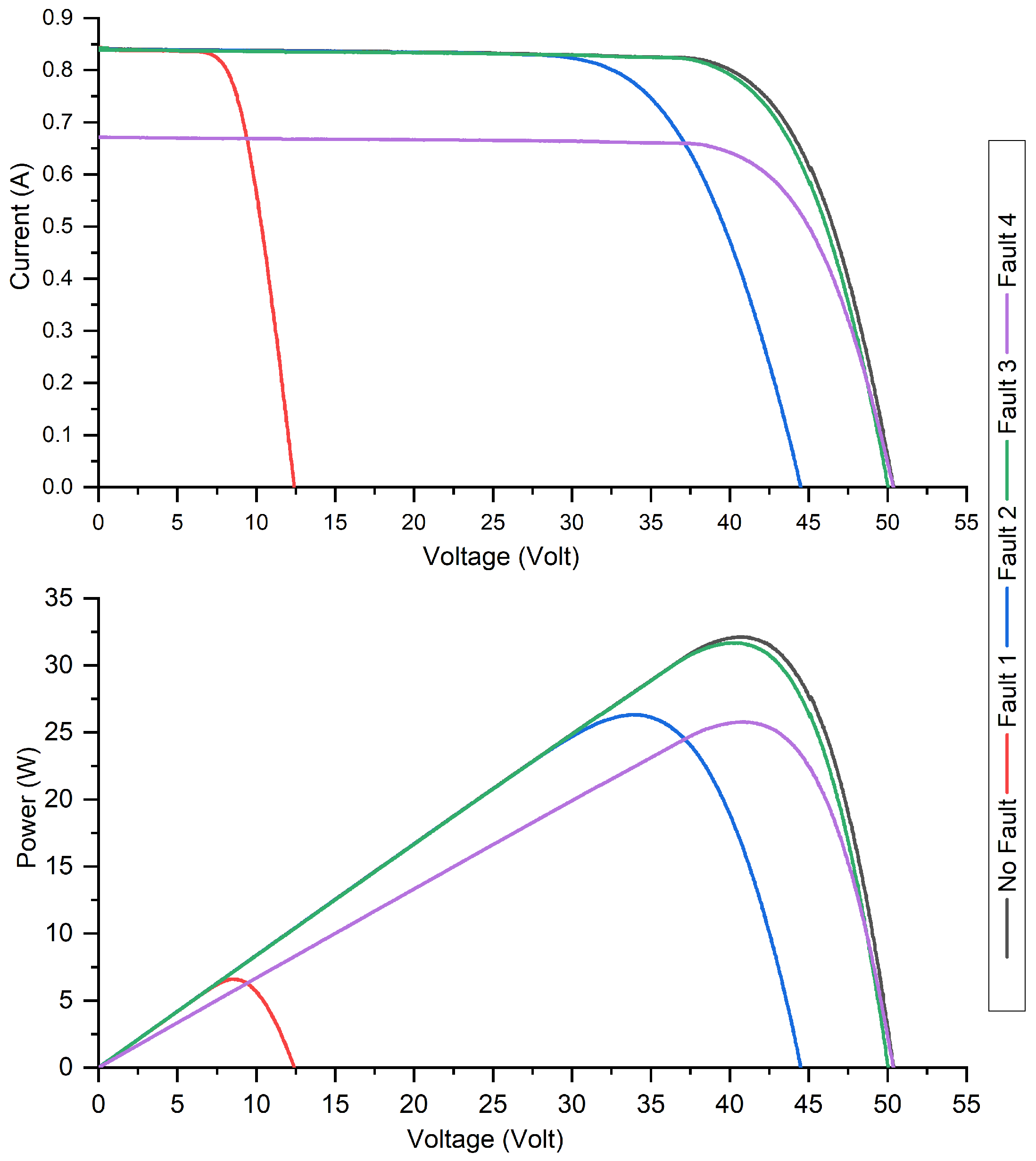
When a system’s performance is evaluated in various scenarios, insights are gained into its efficiency. In the F1 scenario, the difference between the healthy and fault condition is clear based on the loss ratio. The efficiency undergoes a significant drooping, resulting in a 63.74% drop when a fault occurs. Conversely, in scenario F2, the overall system efficiency diminishes from 80.31% under healthy conditions to 65.81% during a fault, resulting in an efficiency loss of 14.50%. For scenario F3, the efficiency decreases slightly, moving from 80.31%, in its optimal state, to 79.22%. This suggests challenges in detecting this specific fault, translating to an efficiency loss of 1.09%. Scenario F4 witnesses a notable reduction in system efficiency. From an initial efficiency of 80.31% under healthy conditions, it drops to 63.45% when the fault occurs, resulting in a 16.86% loss. Figure 6 provides further clarity: there is a pronounced drop in the power output during F1, while F3 shows only a marginal reduction in PV power compared to regular functioning.
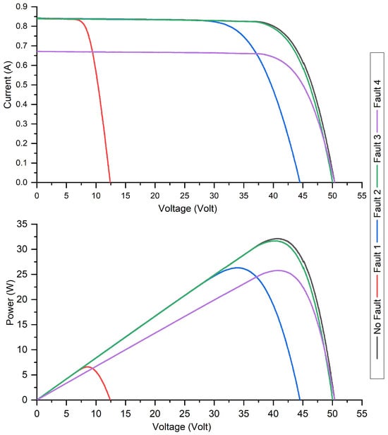
Figure 6.
IV and PV curve under the normal and faulty conditions.
3. Proposed Fault Diagnosis Method
Within this section, the authors present a comprehensive examination of two detection methods proposed for fault detection and classification in PV systems. These methods are built upon Support Vector Machines (SVMs) and Extreme Gradient Boosting (XGBoost). Additionally, an optimization algorithm is applied to fine-tune the classifier’s parameters for enhanced performance in fault detection and classification.
3.1. Particle Swarm Optimization (PSO)
The Particle Swarm Optimization (PSO) algorithm, conceived by Eberhart and Kennedy [27], is a resilient metaheuristic approach rooted in the behavior of particles and social creatures, such as birds, within a swarm. Each particle (candidate solution) adjusts its position based on its own experience and that of its neighbors. This mimics the social behavior of birds or fish adjusting their paths based on their own experience and the experience of their fellow creatures. PSO effectively addresses a plethora of optimization challenges, with each particle embodying a potential solution. The methodology to pinpoint the ideal solution is delineated in the following steps [28]:
- (a)
- Initialization: Begin with the initial population of particles and set their corresponding velocities. Subsequently, evaluate the fitness of each particle and determine the optimal positions, designating them as the global best and local best.
- (b)
- Update Velocity: During each iteration, each particle navigates through the search space with a designated velocity. In each cycle, this velocity is influenced by two primary factors: the global best and the local best. While the global best represents the particle’s finest position achieved thus far, the local best signifies the optimal solution within the current iteration.
- (c)
- Update Particle Position: Once the new velocity is calculated, the particle’s movement through the search space is adjusted accordingly. This involves the particle moving with its updated velocity. The adjustment in the velocity of each particle is governed by Equation (1).where and denote the position and velocity of the (jth) particle at the (ith) iteration, respectively; stands for the inertial weight coefficient; is the iteration number; and and stand for numbers in the interval .
- (d)
- Update the global best and local best: If the newly modified particle shows the best values, both the global and local best values will be updated accordingly. The method for updating the local best for each particle is governed by Equation (2).
- (e)
- Evaluate Termination Criteria: When the specified stopping criteria are fulfilled, the global best solution is returned as the optimal resolution for the specific problem. In case the termination criteria are not met, the process returns to the Update Velocity step.
3.2. The Bees Algorithm
The Bees Algorithm is a recent technique proposed by a research team within the Center for Manufacturing Engineering at Cardiff University, and it works by evaluating the effectiveness of a population search algorithm [29]. The BA copies the foraging behaviors of a swarm of honeybees and can be described as belonging to the “intelligent optimization tool” group. In other words, BA replicates the behavior of honey bees by specifying some conditional parameters to start the simulation. BA encompasses six parameters that need to be tuned to ensure a proficient and congruent search for the best primary variables, namely:
- Scout bee numbers ;
- Selected bee numbers ;
- Elite bee numbers ;
- Numbers recruited for elite locations ;
- Numbers recruited from the best differing locations ;
- Patch size for neighborhood localized search .
The exploration begins by spreading a set number of scout bees randomly throughout the search space. Sites visited by these scouts are evaluated based on an objective function and ranked in an ascending or descending sequence, contingent upon the optimization function to minimize or maximize the process. From this ranking, the highest fitness value locations are chosen as the selected sites , and the bees visiting these sites are chosen to perform neighborhood searches. For this neighborhood search, the selected sites are further divided into two categories: elite sites and non-elite sites . Subsequently, the algorithm performs a neighborhood search around the selected sites by assigning more forager bees to search near to the elite sites and fewer bees to investigate the vicinity of the non-elite sites . These parameters can be calculated as follows [30,31,32]:
Equation (3) is the first condition that must be satisfied. The size of the bees’ population, p, can be calculated using Equation (4). The equation for finding the random scouting bees during the initialization phase, as well as the unselected bees, can be written as:
In the given context, “rand” represents a random vector element between 0 and 1, and and denote the lower and upper bounds of the solution vector, respectively. For recruiting bees during the neighborhood search:
Lastly, the BA optimization can be defined as a process of searching to identify the most optimal solution to a given challenge. This can be described mathematically as:
where f is the objective function(s); x is the parameter (decision variable (s)) that needs to be optimized, and it can be continuous, discrete, or a mixture of both. By using the BA optimization technique, it is possible to quantitatively measure a system’s performance, subject to some constraints on the ranges of the variables.
3.3. Support Vector Machines (SVMs)
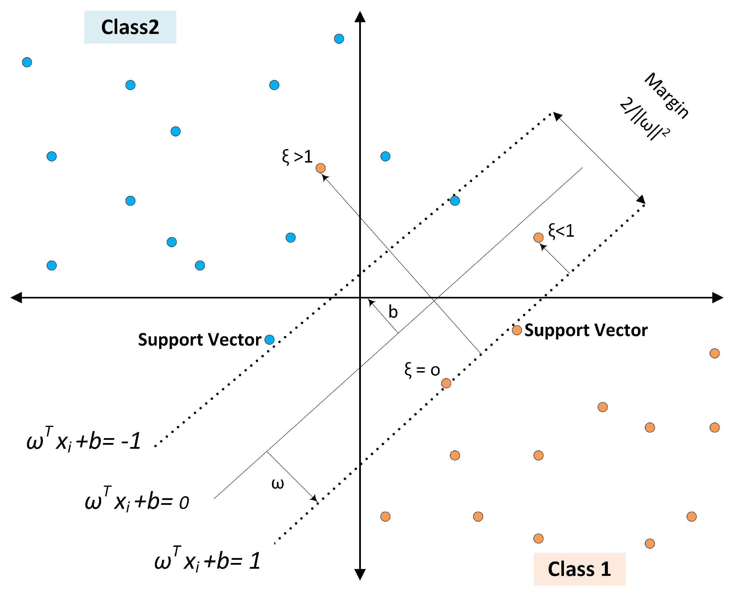
The original support vector classifier was introduced by [33] as a two-class system. Nowadays, Support Vector Machines (SVMs) are viewed as an optimal solution for supervised learning, as they focus on identifying a hyperplane that maximizes the distance between two adjacent classes. This maximization aids in limiting the generalization error of the classification model. In Figure 7, classes are linearly separated, and the distance between the decision boundary and the nearest training patterns is the margin. This margin is defined by support vectors that determine the classification functions. If the data points cluster and cannot be separated linearly, they can be remapped to a higher dimension where they are linearly separable using a hyperplane, as discussed in [34]. The Support Vector Machine classifier is derived as shown below:
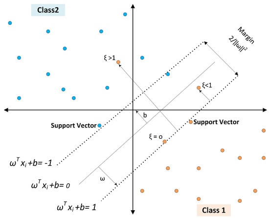
Figure 7.
Maximum margin classification with Support Vector Machines.
N-dimensional inputs ), where m represents the number of samples in either class one or two, are labeled for the first class and for the second class. When the data are linearly separable, a hyperplane is identified to separate the data.
in which represents an n-dimensional vector, with b representing an intercept term. The hyperplane which separates the two vectors is positioned based on those vectors and meets the constraint where and if , thus forming a functional margin:
The optimal separating hyperplane is defined as the hyperplane that leaves the greatest distance separating the plane from the closest data point, and this is illustrated in Figure 7. Calculation of the geometric margin gives . Accounting for noise through as the variable for slack, and, with , as an error penalty, the optimal hyperplane is determined through applying a convex quadratic optimization problem, as follows:
In Equation (10), the minimization of is synonymous with minimizing . Furthermore, Equation (11) describes a quadratic programming problem, which is formalized into the Lagrange formula by incorporating both the objective function () and the constraints .
It is now possible to form the Lagrangian:
To find , the Lagrangian problem of duality must be solved. Considering an SVM-derived two-class problem, a decision boundary is given in the following, which uses the kernel function of a new pattern (for classification) and as the training pattern:
in which each equal 0, with the exception of support vectors. The Radial Basis Function (RBF) is chosen as the kernel function of the SVM in this research, which can be described:
3.4. Extreme Gradient Boosting (XGBoost)
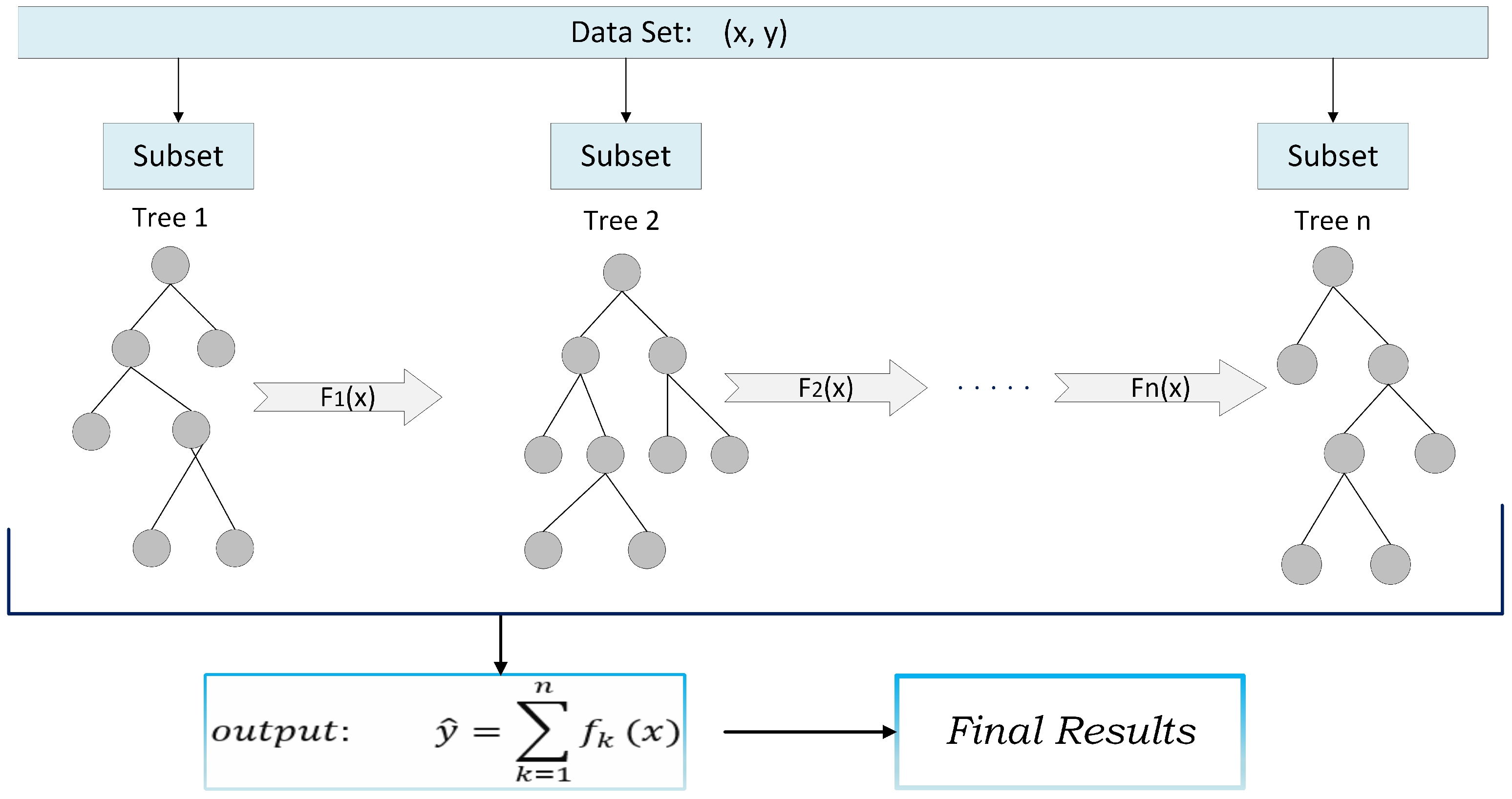
XGBoost, short for Extreme Gradient Boosting, provides an efficient and adaptable rendition of the gradient boosting methodology framework by [35,36]. XGBoost, a highly efficient variant of the gradient tree boosting algorithm, has recently garnered significant attention largely due to its outstanding results in Kaggle competitions. Central to XGBoost’s success is its adaptability across diverse scenarios and its swift computational capabilities, as outlined by [37]. The algorithm leverages bagging (bootstrap aggregation) and random feature selection, which not only combats the risk of overfitting but also aptly balances the bias–variance trade-off. Owing to these unique benefits, XGBoost has emerged as a preferred choice in studies focusing on fault diagnostics in solar power systems [38,39]. The predicted output of XGBoost is the sum of all the results, as shown in Figure 8. It can be used for both regression and classification problems. The working principle of the XGBoost is as follows:
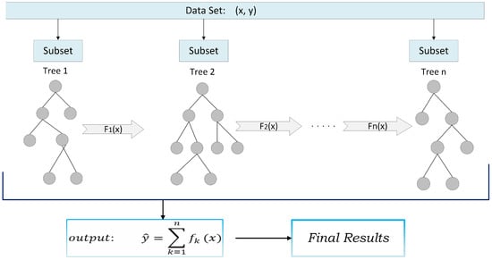
Figure 8.
A general architecture of XGBoost.
Given a training dataset, D, consisting of i samples and j features, where x represents the input variables and y denotes the output variables, the dataset can be represented as shown in Equation (18). The culmination of the XGBoost training process results in a model composed of the summation of the K CART (Classification and Regression Tree) decision tree functions, as described by [40].
In this context, , denotes the feature j of the sample i. represents the output of the XGBoost model, F symbolizes the collection of CART decision trees, corresponds to a tree, so is the result of tree k. Each CART decision tree consists of a tree structure, denoted as q, and T leaf nodes. Every leaf node j has a continuous value corresponding to it, which is termed the weight of the leaf node. The weight vector w is an assembly of the weights from all leaf nodes. The objective of XGBoost is:
In supervised learning, a loss function is utilized to quantify the discrepancy between the model’s predicted values and the actual values. The loss function for the XGBoost model can be articulated as:
where is loss function, is the prediction, is the target, is the regular terms, and penalizes the complexity of the model.
The model is trained using an additive approach, where the prediction for the i-th instance at the t-th iteration, denoted as , can be represented as:
In this situation, it minimizes the following objective:
To accelerate the optimization of the objective, the method of second-order approximation is employed as follows:
where and represent the first- and second-order gradient statistics on the loss function, respectively.
4. Classification Accuracy, Sensitivity, and Specificity Analysis
The classifiers are assessed to understand how well they perform, using a confusion matrix to calculate specific metrics. The most significant aspect of performance is accuracy, based on the extent to which classifications are correct. Further metrics applied are recall and precision [41], and their respective definitions are given below:
TP represents the number of True Positive classification results, indicating how many samples should fall into the “x” classification and are correctly identified by the classifier. FN gives the number of False Negatives, which are samples that should be classified as “” but have been given a different classification. The number of True Negatives is given by TN and indicates how many samples that should not be in class “x” have been classified as not in class “”. FP indicates the number of False Positives, which are samples incorrectly identified by the classifier as belonging to class “x” when this is not their real category. The term d gives the number of samples in the test set. A further metric that is frequently added to the previous metrics when evaluating the classifiers’ performances is the confusion matrix, sometimes termed the contingency table. This metric provides a definitive and simple approach to representing the findings from classifications. This matrix shows binary classification problems through a two-row, two-column matrix. The meaning of the confusion matrix is shown in Table 6.
Table 6.
Confusion matrix for the performance evaluation of learning algorithms.
5. Implementation Proposed Methods
To evaluate the efficacy of the proposed fault diagnosis approach, an empirical study was undertaken. The experimental setup employed a desktop computer equipped with an Intel(R) Core(TM) i7-10700 central processing unit (CPU) operating at 2.90 GHz and bolstered by 32.0 GB of RAM. The diagnostic methods were coded in the Python programming language. Rapid execution of the method was enabled through the use of specialized modules tailored for Machine Learning algorithms, optimizers, and cost functions.
5.1. Implementation of SVM
In this study, a dataset of labeled samples from the PV array is carefully collected, where each sample represents a specific observation from the PV system and is labeled as either normal or faulty. Before training the SVM model, data preprocessing steps, such as data cleaning and feature scaling, are performed to enhance model performance and ensure that all features have equal significance during training. To evaluate the SVM model’s performance, the dataset is divided into a training set (80% of the data) used to teach the SVM model and a 20% testing set used to assess the model’s ability to generalize to unseen data. Since the PV dataset is nonlinear, the SVMs were trained using a non-linear Radial Basis Function kernel through LIBSVM. Fine-tuning and (gamma) are of the utmost importance when utilizing a Support Vector Machine (SVM) for fault detection in PV arrays. These parameters directly influence the SVM model’s ability to accurately classify samples and its robustness in handling unseen data. In SVMs, acts as a regularization parameter, and “gamma” serves as the kernel coefficient parameter, which is especially crucial for non-linear kernels such as the Radial Basis Function kernel. determines the trade-off between maximizing the margin of the decision boundary and minimizing the classification errors on the training data. Ultimately, the effectiveness of the SVM model is assessed using common evaluation metrics such as the root-mean-square error (RMSE) and confusion matrix.
Support Vector Machine-Based Hybrid Expert Systems
Hybrid techniques have emerged as a compelling approach by amalgamating two distinct fault detection methods into a single algorithm. These techniques have found application in fault detection within photovoltaic (PV) systems with the overarching objectives of: (1) Enhancing the precision of fault detection; (2) Mitigating the computational load, (3) Facilitating precise differentiation between faults that share similar characteristics; and (4) Enabling the identification of multiple instances of faults. Support Vector Machine (SVM)-based hybrid expert systems are intelligent systems that merge the principles of SVM with other methodologies or techniques. Their goal is to enhance performance, especially in the decision-making and predictive analysis domains. To ensure the best selection of hyperparameters, two optimization strategies, the Bees Algorithm (BA) and Particle Swarm Optimization (PSO), are implemented.
- (a)
- Parameter optimization of SVM based on PSO
Swarm intelligence algorithms are commonly employed in simulations to tackle problems involving multiple local extrema. The PSO algorithm, which models social behaviors, such as bird flocking, stands as an exemplar of swarm intelligence. The combined variable of the SVM penalty factor and the RBF kernel parameter is used as the search target of the PSO algorithm so as to find the combinatorial variable value that has the highest classification accuracy of an SVM. As previously mentioned, the parameters to be optimized are (C, ). These parameters should be restricted in order to guarantee the learning capacity and generalization capacity of the model. The optimization problem is formulated as:
where and represent the predicted and actual output of the model, and n represents the number of samples in the dataset.
The PSO algorithm employs particles that move through the hyperparameter space to identify the best set of hyperparameters that minimize the error rate of the SVM classifier on the test dataset. The movement of each particle is influenced by its own best-known position and the global best-known position found by any particle in the swarm. Table 7 presents the configuration of the PSO parameters specifically designed for PV fault detection. PSO is established with a simpler architecture, and the process for constructing a PSO-SVM model is detailed in Algorithm 1.
| Algorithm 1 Pseudocode of PSO-SVM. |
|
Table 7.
Default parameters of PSO algorithm for SVM parameter optimization.
- (b)
- Parameter optimization of SVM based on BA
The Bees Algorithm (BA), inspired by the foraging behavior of honey bees, is employed to optimize the hyperparameters of Support Vector Machines (SVMs). First, “scout bees” explore the SVM hyperparameter space, encompassing potential values for parameters such as the penalty parameter C and the gamma parameter if using an RBF kernel. Through a process similar to bees evaluating nectar quality, each scout evaluates the performance of the SVM for its specific hyperparameters, typically via cross-validation. Based on preliminary evaluations, the best-performing hyperparameter combinations, termed “sites”, are identified. A subset of these sites is distinguished as “elite” due to their superior performance metrics. By drawing parallels with how bees swarm richer nectar sources, other bees are “recruited” to further investigate these promising sites. Elite sites naturally attract more bees than non-elite sites, confirming the search around the hyperparameters that already show promise. As the bees further scrutinize the surroundings of these sites, they may discover better combinations of hyperparameters, thus updating the site’s coordinates. However, if certain locations consistently perform poorly over many iterations, they will be “abandoned”, leading to the initialization of new scouts in different regions of the hyperparameter landscape. This mechanism ensures that the BA is not overly focused on local optima, promoting large-scale exploration. As the algorithm progresses, it exhibits a pattern of discovery, mobilization, improvement, and intermittent stopping. It reaches convergence either after a predetermined number of iterations or when no further performance gains are observed, ultimately determining the best-suited SVM hyperparameters.
Finally, Table 8 shows how the parameters for the Bees Algorithm were set to find the optimal SVM parameters for enhancing the PV fault detection accuracy. However, if the optimization goal is modified to search for different optimal parameters, the optimization parameters must be modified to match the new search criteria. Algorithm 2 details the procedure to construct a BA-SVM model.
| Algorithm 2 Pseudocode of BA-SVM. |
|
Table 8.
Default parameters of BA algorithm for SVM parameter optimization.
5.2. Implementation of XGBoost
XGBoost offers a set of superior parameters that can be tuned to optimize its performance. One of the primary parameters is the learning rate, or ‘eta’, which controls the step size at which the boosting process adjusts the weights of weak learners. The model’s complexity is dictated by the number of boosting rounds or trees, denoted as ‘n-estimators’. The tree’s depth, given by ‘max-depth’, determines how deep each tree can grow, with deeper trees resulting in more complex models. On the other hand, ‘subsample’ determines the fraction of samples and features used to build each tree, to prevent overfitting. For the maximum tree depth, greater values produce results that are more specific to localized samples. The ‘gamma’ parameter introduces regularization by specifying the minimum loss reduction necessary to create an additional partition on the terminal node, and ‘min-child-weight’ specifies the minimum sum of the instance weight required in a child node, preventing overly fine-grained partitioning. On the other hand, ‘reg-lambda’ provides L2 regularization on the model’s weights to prevent over-fitting.
Another noteworthy aspect is the possibility of ‘early-stopping-rounds’, which enables the training to halt if the model’s performance on a validation set starts deteriorating. Furthermore, when validating the model, the number of folds for cross-validation can be determined using ‘num-folds’. Due to the interaction between these parameters, it is beneficial to employ methods such as grid search or random search to identify the optimal hyperparameter set for a specific problem. The information of each parameter is shown in Table 9. However, “Default values” denote the initial settings that XGBoost uses if not explicitly altered. When using XGBoost without customizations, it adopts these values. Although these defaults are based on standard scenarios and often yield decent results, adjusting them can enhance the performance for particular tasks ordatasets [42,43].
Table 9.
Tuning XGBoost model hyperparameters.
5.3. XGBoost-Based Hybrid Expert Systems
Optimizing hyperparameters is essential to improving XGBoost’s performance. By incorporating optimization techniques directly into the XGBoost model, one can systematically explore its hyperparameter space. This effort not only aims to boost the model’s accuracy but also to enhance its predictive capabilities, allowing superior predictive results to be obtained at significantly lower computational time and cost.
- (a)
- Parameter optimization of XGBoost based on PSO
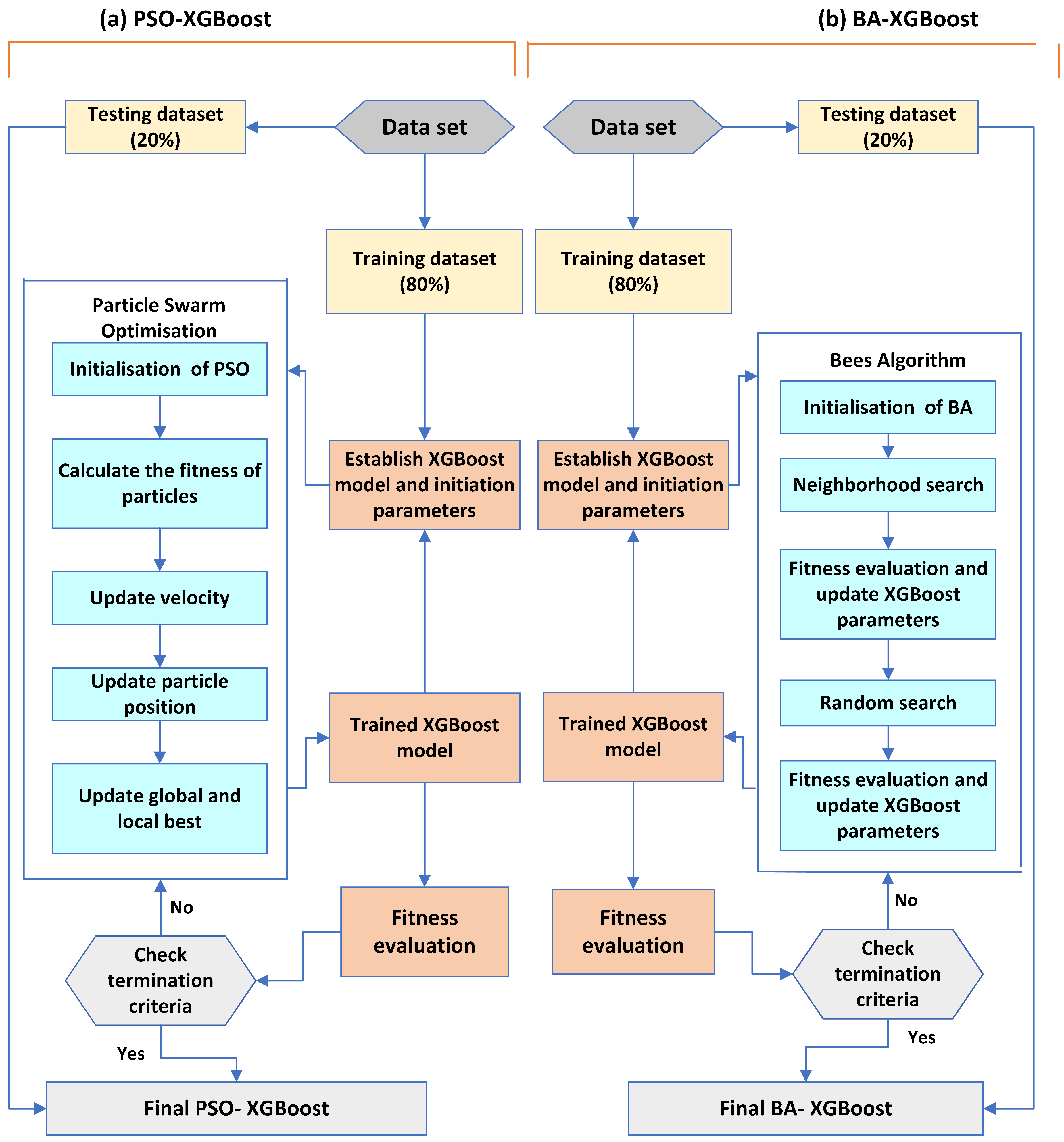
In this study, XGBoost serves as the basic model for fault detection in the PV array, while the PSO approach plays a pivotal role in optimizing the hyperparameters of the XGBoost model. The comprehensive optimization technology involves optimizing seven parameters that affect the control quality of the XGBoost model. To determine the optimal XGBoost model using the PSO algorithm, a fitness function described in Equation (29) is employed. The flowchart illustrating the proposed PSO-XGBoost model for PV array fault detection is depicted in Figure 9a. Initially, an XGBoost model was developed using the training dataset. Subsequently, the PSO algorithm was employed to tune the hyperparameters of the XGBoost model. Within the PSO algorithm, there are several parameters that drive the optimization process. This includes the population size , the maximum number of iterations , the maximum velocity of particles , the individual cognitive coefficient , the group cognitive coefficient , and the inertia weight .
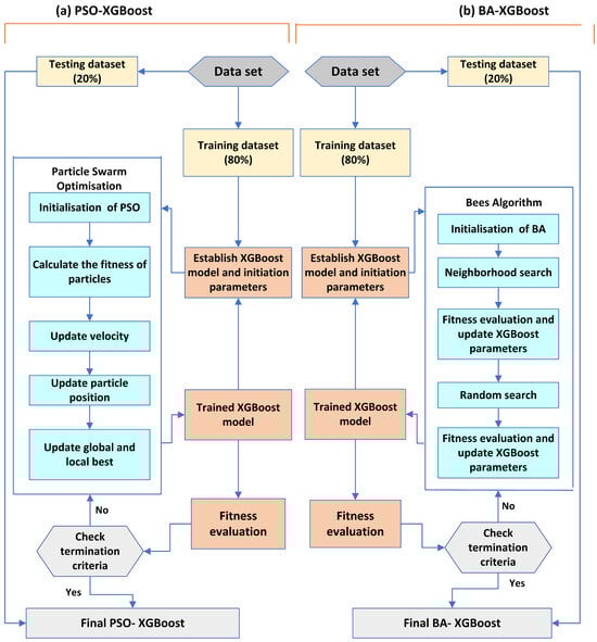
Figure 9.
Flowchart of XGBoost framework: (a) PSO-XGBoost model; (b) BA-XGBoost model.
The PSO begins by initializing a population of particles. Each of these particles represents a unique set of XGBoost hyperparameters, which include values such as the learning rate, maximum depth, and regularization terms. Once initialized, the XGBoost model for each particle is trained, and its performance is evaluated using a fitness function. This function, typically based on a validation dataset, quantifies the model’s performance with the current hyperparameter set.
In this process, each particle keeps track of the best set of hyperparameters it has encountered based on a fitness function, known as its “personal best”. In addition, the best-performing hyperparameter combination across all particles is identified as the “global best”. As particles navigate the hyperparameter space, their movement or “velocity” is affected by two main factors: their own personal best and the global best. These attractions, along with inertia, determine how particles adjust their velocities, with parameters such as inertial weight and cognitive and social parameters controlling their influence. With modified velocities, the particles’ positions in the hyperparameter space change, effectively changing the hyperparameter values. This iterative process of adjusting velocities and positions continues until convergence is achieved. Convergence is usually determined by a specific stopping criterion, such as when the improvement to the global best becomes negligible.
Once convergence is achieved, the XGBoost model is trained using the best set of hyperparameters found, which is the global best, on the entire training dataset. Finally, to ensure that the optimized model performs well in real-world scenarios, its performance is evaluated on a separate test dataset. The specific parameters used in PSO can be referred to in Table 10. The default parameters and typical search spaces for XGBoost optimization are illustrated in Table 11 while Algorithm 3 offers the basic pseudocode of the PSO-XGBoost model.
| Algorithm 3 Pseudocode of PSO-XGBoost. |
|
Table 10.
Default parameters of PSO algorithm for XGBoost parameter optimization.
Table 11.
Default parameters and typical search spaces for XGBoost optimization.
- (b)
- Parameter optimization of XGBoost based on BA
The flowchart illustrating the proposed BA-XGBoost model for PV array fault detection is depicted in Figure 9b. In this optimization model, a population of scout bees is initially launched where each bee has a unique set of XGBoost parameters derived from the specified ranges. For instance, a scout might be assigned a max_depth of three, a gamma of 0.5, and n_estimators set to 500. Each of these scout bees then gauges the fitness of its designated parameters. This fitness assessment usually involves training the XGBoost model with the given parameters, using techniques such as cross-validation, and then recording relevant performance metrics, such as the accuracy or RMSE, as mentioned in Equation (29).
After scouts calculate their fitness scores, the most promising parameter combinations, those that achieve superior model performance, are classified as “promising sites”. Within this elite group, some sites stand out more due to their exceptional fitness values and are therefore termed “elite sites”. The BA then dispatches a larger group of bees to examine these elite sites more closely. These bees fine-tune the parameters, exploring the nearby hyperparameter space to see if any neighboring group might provide better results. Conversely, promising non-elite sites attract a smaller group of bees for a similar exploratory mission. To ensure a comprehensive survey of the hyperparameter landscape, some bees are dispatched to randomly traverse the vast parameter space, safeguarding against an undue concentration on local regions and facilitating broader exploration.
As this dynamic is repeated, the algorithm progressively improves the hyperparameters. The iterative cycle continues either for a predetermined number of cycles or until the XGBoost model’s performance improvements reach a plateau. At the conclusion of this regimen, the algorithm accurately identifies the bee with the highest fitness score and provides the optimal set of parameters to the XGBoost model for the data in question. Through the BA, the focus has been on promising regions in the hyperparameter space, providing a more efficient alternative to exhaustive grid searches, especially in light of the multifaceted nature of XGBoost hyperparameters.
Table 12 illustrates how the parameters for the Bees Algorithm were set to find the optimal XGBoost parameters for enhancing its ability to accurately detect photoelectric faults. Conversely, Table 11 displays the default parameters and common search spaces for XGBoost optimization. However, if the optimization target was to be modified to search for different optimal parameters, the optimization parameters would need to be adjusted to match the new search criteria. Algorithm 4 outlines the procedure for building a BA-XGBoost model.
| Algorithm 4 Pseudocode of BA-XGBoost. |
|
Table 12.
Default parameters of BA algorithm for XGBoost parameter optimization.
6. Results and Discussion
The performance of the proposed methods, SVMs and XGBoost, has been assessed in terms of detection accuracy. These methods are further enhanced by integrating nature-inspired algorithms, specifically the Bees Algorithm (BA) and Particle Swarm Optimization (PSO), with the aim of improving the model’s efficacy and accuracy. Figure 10 displays a confusion matrix that illustrates the performance metrics of the SVM, SVM-PSO, and SVM-BA, while Figure 11 provides confusion matrix details regarding the classification outcomes achieved by XGBoost, XGBoost-PSO, and XGBoost-BA. The results for the standard SVM and XGBoost techniques, together with the newly introduced optimization strategy for these classification methods, are illustrated in Figure 12.
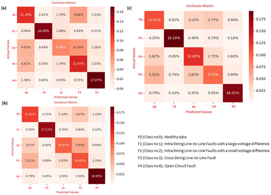
Figure 10.
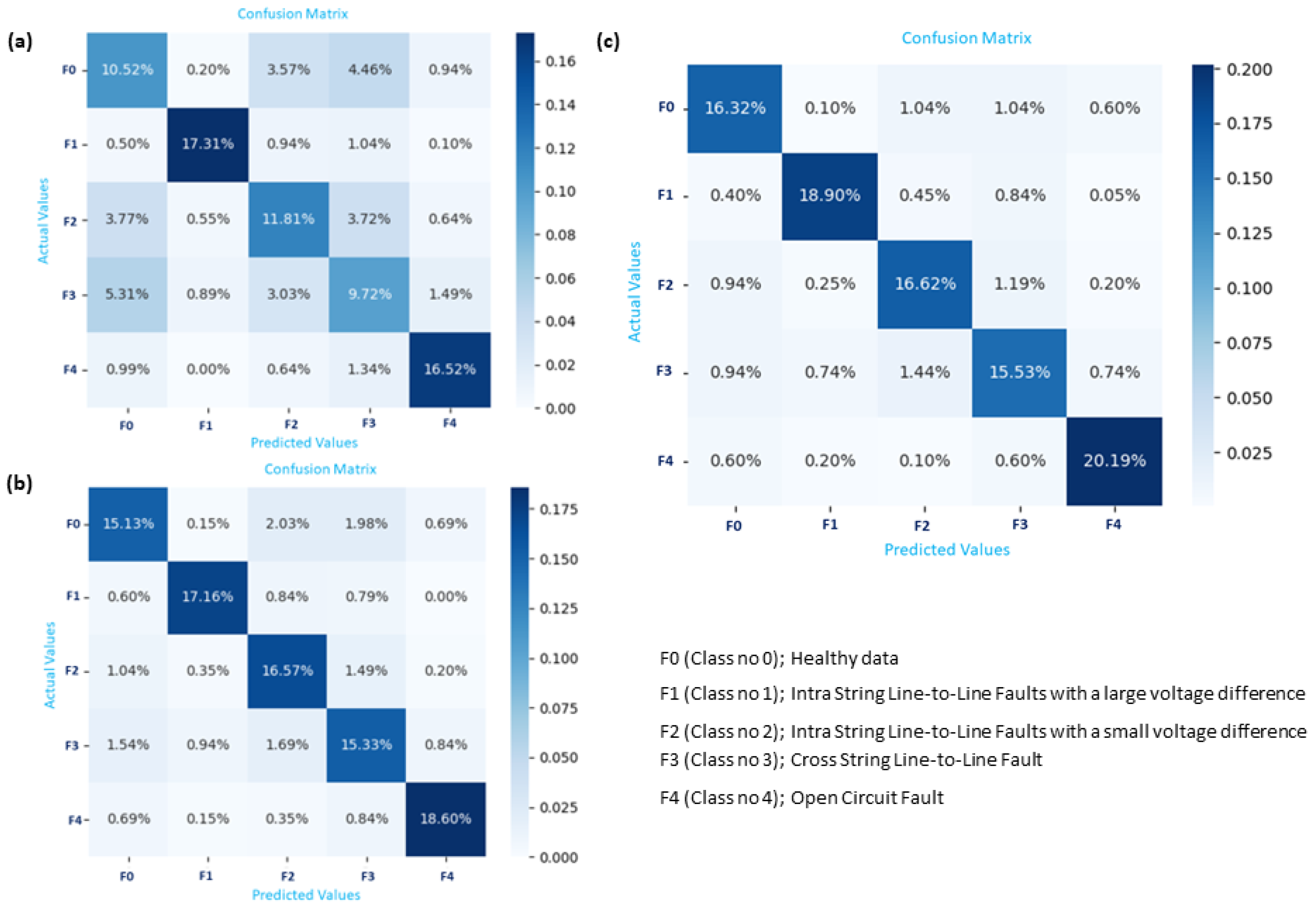
Confusion matrix illustrating fault identification based on classifiers: (a) SVM, (b) SVM-PSO, and (c) SVM-BA.

Figure 11.
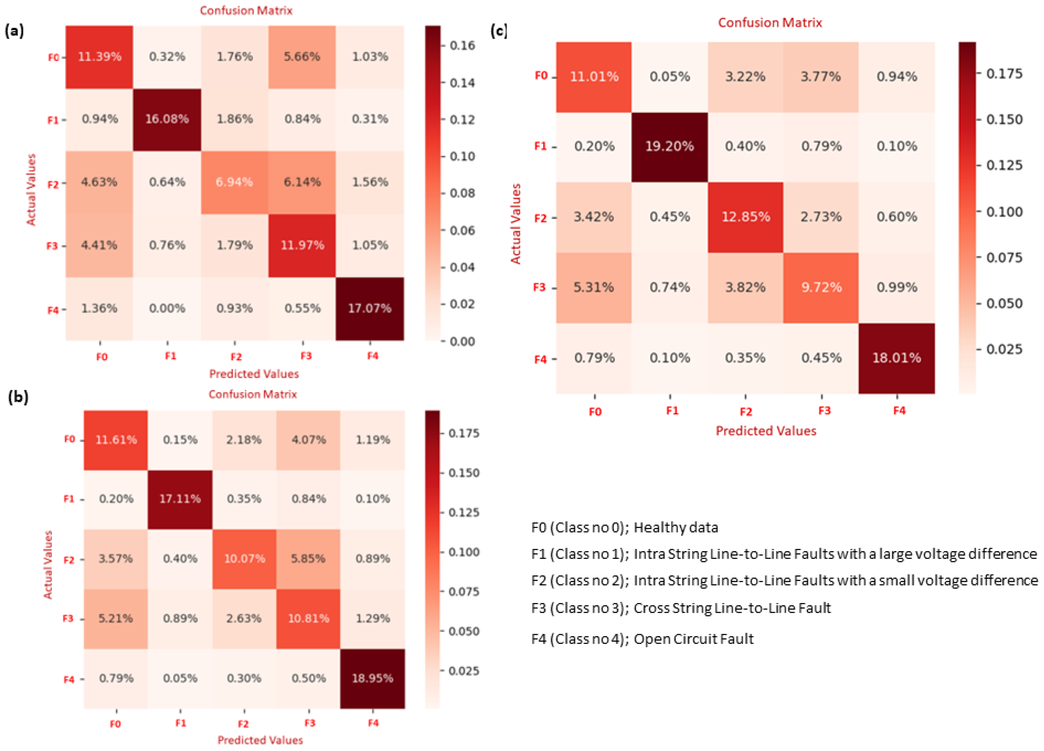
Confusion matrix illustrating fault identification based on classifiers: (a) XGBoost, (b) XGBoost-PSO, and (c) XGBoost-BA.
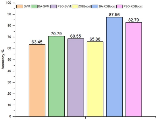
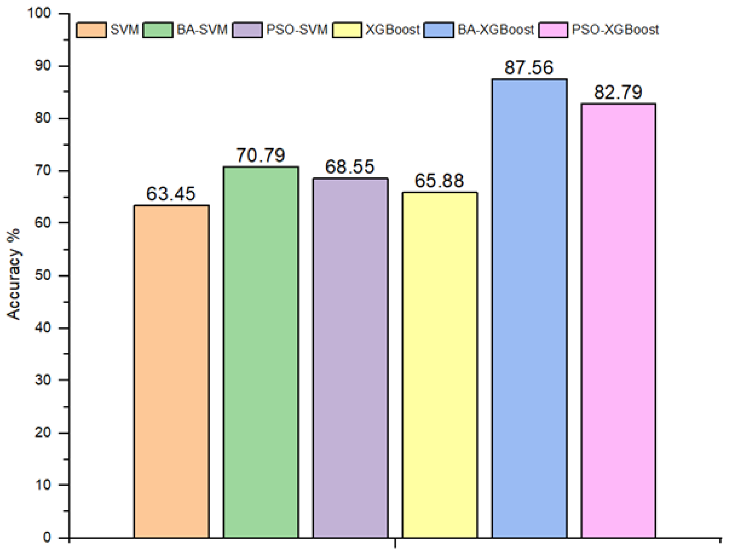
Figure 12.
Assessed outcomes of the proposed methods in terms of overall precision.
As shown in Table 13, an insightful comparison of different Machine Learning classifiers is provided, demonstrating their effectiveness in detecting faults in a small-scale photovoltaic (PV) system as described in Section 2. Each classifier’s efficacy is evaluated based on its accuracy in detecting specific fault types and its overall accuracy. In the provided data, five scenarios are outlined: F0 represents a healthy condition; F1 and F2 denote intra-string line-to-line faults, with F1 characterized by a large voltage difference and F2 by a small voltage difference; F3 is identified as a cross-string line-to-line fault; and F4 signifies an open-circuit fault. In order to ensure the fairness of the experiment and comparison between the proposed classifier methods, while taking into account the accuracy and computational complexity of the model, the number of iterations of the hyperparametric algorithm is set to 100 for each classifier.
Table 13.
Comparison of the performance assessment between proposed methods.
In the context of a confusion matrix evaluating the performance of a classification model, as shown in Figure 10a, FP represents the count of False Positives (6.14%). These instances denote samples incorrectly classified by the model as belonging to class F3 but should be categorized as F2. Notably, F1 achieves the highest accuracy. Looking at Figure 10c, it is evident that the classifier BA-SVM shows a significant improvement, with F2 registering a 12.85% classification rate. Examining the classification metrics in greater detail improves the comprehension of the BA-XGBoost system’s performance, as shown in Figure 11c and illustrated in Table 14. The F3 fault had its own challenges: it was correctly classified at 15.53%, but there was a notable 3.86% rate of misclassification, yielding a user accuracy of 80.09%. Among all, the F4 fault stood out by achieving the highest accuracy. It was correctly classified at 20.19% and misclassified at a mere rate of 1.5%, resulting in a user accuracy of 93.08%.
Table 14.
Classification results of the hybrid BA-XGBoost method for the testing data using confusion matrices.
An evaluation of the performance of various classifiers is presented in Table 13. Among the classifiers, BA-XGBoost emerges as the most proficient, achieving an overall accuracy of 87.56%. This indicates its superior ability to correctly classify different types of faults. PSO-XGBoost is another standout, displaying an overall accuracy rate of 82.79%. Traditional SVM, while not the most advanced, holds an overall accuracy of 63.45%. PSO-SVM and XGBoost are also noteworthy, posting overall accuracies of 68.55% and 65.88%, respectively. In terms of user accuracy for specific fault types, SVM, XGBoost, PSO-SVM, and BA-SVM show particularly low sensitivity in detecting F0, F2, and F3 faults. On the other hand, BA-XGBoost provides a balanced performance across the various fault types. Diving deeper into the classification metrics provides a clearer picture of the system’s performance, as shown in Figure 10 and Figure 11. The F3 fault had its own challenges; it is evident that there is a significant misclassification between the categories of F0 and F3. This can be attributed to the data similarity between the two classes, which leads to reduced accuracy in classification. While the computational times for all compared methods to detect and classify PV faults with the number of features considered, the proposed hybrid BA-SVM and BA-XGBoost are observed to have higher computational times, followed by PSO-SVM, PSO-XGBoost, SVM, and XGBoost, around 3.2, 2.56, 1.69, 0.91, 0.17, and 0.09 min, respectively. However, the proposed hybrid BA-XGBoost establishes itself as the most accurate ML technique for fault diagnosis; all five ML techniques perform better than the BA-XGBoost in terms of computational time speed.
In the continuous pursuit of enhancing renewable energy technologies, when detecting faults within small-scale photovoltaic systems, the application of optimization techniques, whether Particle Swarm Optimization (PSO) or the Bees Algorithm (BA), considerably elevates the performance of base classifiers such as SVM and XGBoost. The results for the standard SVM and XGBoost techniques, together with the newly introduced optimization strategy for these classification methods, are illustrated in Figure 12. Specifically, BA-XGBoost stands out with the most impressive overall accuracy among the presented methods. This suggests that the Bees Algorithm, in this context, offers significant advantages for parameter optimization, potentially leading to more accurate and reliable fault detection outcomes in PV systems.
7. Conclusions
This paper highlights the imperative need for advanced fault detection techniques in PV systems. In a bid to enhance the accuracy and dependability of Machine Learning classifiers, a small-scale PV system was designed and constructed. This experimental setup was carefully designed to mimic the complexities of real-world solar systems. By intentionally introducing certain faults within the arrays, various challenges that these systems would face in real-world operations were simulated. The primary motivation for this endeavor was to create a robust dataset, both comprehensive and rooted in realistic scenarios. Such high-quality training data are vital, especially for the Machine Learning algorithms deployed. The addressed faults include line-to-line faults in different scenarios and open-circuit fault , and tests were conducted in accordance with established standard testing conditions. By utilizing the power of Machine Learning, specifically through Support Vector Machines (SVMs) and Extreme Gradient Boosting (XGBoost), the research successfully demonstrated the capabilities of these techniques in accurately identifying a multitude of fault conditions present in PV arrays. To further improve their accuracy in PV fault detection, this paper introduces two optimization algorithms: Particle Swarm Optimization (PSO) and the Bees Algorithm (BA). The primary goal is to improve the model’s precision and overall performance. The evaluation of these fault detection and classification methods utilizes metrics such as accuracy and confusion matrices. Among the methods compared, BA-XGBoost shows the highest accuracy in detecting different types of faults and overall performance, making it the recommended choice for fault detection in PV systems. The findings put forth a persuasive case for the Bees Algorithm’s resilience and efficiency. The SVM and XGBoost classifiers optimized using BA demonstrated exceptional accuracy in detecting complex PV array faults, achieving 70.79% and an impressive 87.56%, respectively. In contrast, classifiers fine-tuned with the PSO algorithm registered a comparatively lower performance, with SVM scoring 68.55% and XGBoost reaching 82.56%. In essence, the Bees Algorithm (BA) had a significant impact on improving the efficiency of the XGBoost classifier, which indicates the possibility of using this technique not only in fault detection within solar energy but also across other domains.
Author Contributions
Methodology, F.S., F.A. and M.P.; software, F.S. and M.P.; validation, F.S., F.A. and M.P.; investigation, F.S. and F.A.; writing—original draft, F.S.; writing—review & editing, F.S.; supervision, F.A. and M.P.; project administration, F.A. All authors have read and agreed to the published version of the manuscript.
Funding
This research received no external funding.
Institutional Review Board Statement
This study does not require ethical approval because it is related to my study.
Informed Consent Statement
Not applicable as this study does not involve humans.
Data Availability Statement
The data presented in this study are available on request from the corresponding author.
Conflicts of Interest
The authors declare no conflicts of interest.
List of Abbreviations
| AC | Alternative Current | ML | Machine Learning |
| AI | Artificial Intelligence | MPP | Maximum Power Point (W) |
| BA | Bees Algorithm | OCF | Open-Circuit Fault |
| DC | Direct Current | Maximum Power Point | |
| FD | Fault Detection | PV | Photovoltaic |
| FDC | Fault Detection Classification | P-V | Power-Voltage |
| FN | False Negative | PVA | Photovoltaic Arrays |
| FP | False Positive | PVS | Photovoltaic System |
| G | Sun Irradiance | SCF | Short-Circuit Fault |
| Current at Maximum Power Point (A) | STC | Standard Test Condition | |
| Short-Circuit Current (A) | Voltage at Maximum Power Point (V) | ||
| I-V | Current–Voltage | Open-Circuit Voltage (V) | |
| LLF | Line-to-Line Fault |
References
- Matemilola, S.; Sijuade, T. Renewable Resource. In Encyclopedia of Sustainable Management; Springer International Publishing: Cham, Switzerland, 2022; pp. 1–6. [Google Scholar]
- Mellit, A.; Tina, G.M.; Kalogirou, S.A. Fault detection and diagnosis methods for photovoltaic systems: A review. Renew. Sustain. Energy Rev. 2018, 91, 1–17. [Google Scholar] [CrossRef]
- Pillai, D.S.; Rajasekar, N. A comprehensive review on protection challenges and fault diagnosis in pv systems. Renew. Sustain. Energy Rev. 2018, 91, 18–40. [Google Scholar] [CrossRef]
- Madeti, S.R.; Singh, S.N. A comprehensive study on different types of faults and detection techniques for solar photovoltaic system. Sol. Energy 2017, 158, 161–185. [Google Scholar] [CrossRef]
- Ghosh, R.; Das, S.; Panizrahi, C.K. Classification of different types of faults in a photovoltaic system. In Proceedings of the 2018 International Conference on Computation of Power, Energy, Information and Communication (ICCPEIC), Chennai, India, 28–29 March 2018; IEEE: Piscataway, NJ, USA, 2018; pp. 121–128. [Google Scholar]
- Arani, M.S.; Hejazi, M.A. The comprehensive study of electrical faults in pv arrays. J. Electr. Comput. Eng. 2016, 2016, 8712960. [Google Scholar]
- Akram, M.N.; Lotfifard, S. Modeling and health monitoring of dc side of photovoltaic array. IEEE Trans. Sustain. Energy 2015, 6, 1245–1253. [Google Scholar] [CrossRef]
- Chen, Z.; Han, F.; Wu, L.; Yu, J.; Cheng, S.; Lin, P.; Chen, H. Random forest based intelligent fault diagnosis for pv arrays using array voltage and string currents. Energy Convers. Manag. 2018, 178, 264–2018. [Google Scholar] [CrossRef]
- Lu, X.; Lin, P.; Cheng, S.; Lin, Y.; Chen, Z.; Wu, L.; Zheng, Q. Fault diagnosis for photovoltaic array based on convolutional neural network and electrical time series graph. Energy Convers. Manag. 2019, 196, 965–2019. [Google Scholar] [CrossRef]
- Chen, Z.; Wu, L.; Cheng, S.; Lin, P.; Wu, Y.; Lin, W. Intelligent fault diagnosis of photovoltaic arrays based on optimized kernel extreme learning machine and iv characteristics. Appl. Energy 2017, 204, 931–2017. [Google Scholar] [CrossRef]
- Chang, H.-C.; Lin, S.-C.; Kuo, C.-C.; Yu, H.-P. Cloud monitoring for solar plants with support vector machine based fault detection system. Math. Probl. Eng. 2014, 2014, 564517. [Google Scholar] [CrossRef]
- Harrou, F.; Dairi, A.; Taghezouit, B.; Sun, Y. An unsupervised monitoring procedure for detecting anomalies in photovoltaic systems using a one-class support vector machine. Sol. Energy 2019, 179, 58–2019. [Google Scholar] [CrossRef]
- Yi, Z.; Etemadi, A.H. Line-to-line fault detection for photovoltaic arrays based on multiresolution signal decomposition and two-stage support vector machine. IEEE Trans. Ind. Electron. 2017, 64, 8546–8556. [Google Scholar] [CrossRef]
- Adhya, D.; Chatterjee, S.; Chakraborty, A.K. Diagnosis of PV Array Faults Using RUSBoost. J. Control. Autom. Electr. Syst. 2023, 34, 157–165. [Google Scholar] [CrossRef]
- Jimenez-Aparicio, M.; Patel, T.R.; Reno, M.J.; Hernandez-Alvidrez, J. Protection Analysis of a Traveling-Wave, Machine-Learning Protection Scheme for Distributions Systems With Variable Penetration of Solar PV. IEEE Access 2023, 11, 127255–127270. [Google Scholar] [CrossRef]
- Sairam, S.; Seshadhri, S.; Marafioti, G.; Srinivasan, S.; Mathisen, G.; Bekiroglu, K. Edge-based explainable fault detection systems for photovoltaic panels on edge nodes. Renew. Energy 2022, 185, 1440–2022. [Google Scholar] [CrossRef]
- Eskandari, A.; Milimonfared, J.; Aghaei, M. Fault detection and classification for photovoltaic systems based on hierarchical classification and machine learning technique. IEEE Trans. Ind. Electron. 2020, 68, 12750–12759. [Google Scholar] [CrossRef]
- Badr, M.M.; Abdel-Khalik, A.S.; Hamad, M.S.; Hamdy, R.A.; Hamdan, E.; Ahmed, S.; Elmalhy, N.A. Intelligent fault identification strategy of photovoltaic array based on ensemble self-training learning. Sol. Energy 2023, 249, 122–138. [Google Scholar] [CrossRef]
- Eskandari, A.; Milimonfared, J.; Aghaei, M. Line-line fault detection and classification for photovoltaic systems using ensemble learning model based on IV characteristics. Sol. Energy 2020, 21, 354–365. [Google Scholar] [CrossRef]
- Hong, Y.-Y.; Pula, R.A. Diagnosis of photovoltaic faults using digital twin and PSO-optimized shifted window transformer. Appl. Soft Comput. 2024, 150, 111092. [Google Scholar] [CrossRef]
- Eldeghady, G.S.; Kamal, H.A.; Hassan, M.A.M. Fault diagnosis for pv system using a deep learning optimized via pso heuristic combination technique. Electr. Eng. 2023, 105, 2287–2301. [Google Scholar] [CrossRef]
- Garud, K.S.; Jayaraj, S.; Lee, M. A review on modeling of solar photovoltaic systems using artificial neural networks, fuzzy logic, genetic algorithm and hybrid models. Int. J. Energy Res. 2021, 45, 6–35. [Google Scholar] [CrossRef]
- Adhya, D.; Chatterjee, S.; Chakraborty, A.K. Performance assessment of selective machine learning techniques for improved PV array fault diagnosis. Sustain. Energy Grids Netw. 2022, 29, 100582. [Google Scholar] [CrossRef]
- Chine, W.; Mellit, A.; Lughi, V.; Malek, A.; Sulligoi, G.; Pavan, A.M. A novel fault diagnosis technique for photovoltaic systems based on artificial neural networks. Renew. Energy 2016, 90, 501–512. [Google Scholar] [CrossRef]
- Kenny, R.P.; Viganó, D.; Salis, E.; Bardizza, G.; Norton, M.; Müllejans, H.; Zaaiman, W. Power rating of photovoltaic modules including validation of procedures to implement IEC 61853-1 on solar simulators and under natural sunlight. Prog. Photovolt. Res. Appl. 2013, 21, 1384–1399. [Google Scholar] [CrossRef]
- Subudhi, B.; Pradhan, R. A comparative study on maximum power point tracking techniques for photovoltaic power systems. IEEE Trans. Sustain. Energy 2012, 4, 89–98. [Google Scholar] [CrossRef]
- Eberhart, R.; Kennedy, J. A new optimizer using particle swarm theory. In Proceedings of the MHS’95. Proceedings of the Sixth International Symposium on Micro Machine and Human Science, Nagoya, Japan, 4–6 October 1995; IEEE: Piscataway, NJ, USA, 1995; pp. 39–43. [Google Scholar]
- Kennedy, J.; Eberhart, R.C. Particle swarm optimization. Encycl. Mach. Learn 2010, 4, 760–766. [Google Scholar]
- Pham, D.T.; Ghanbarzadeh, A.; Koç, E.; Otri, S.; Rahim, S.; Zaidi, M. The bees algorithmâa novel tool for complex optimisation problems. In Intelligent Production Machines and Systems; Elsevier: Amsterdam, The Netherlands, 2006; pp. 454–459. [Google Scholar]
- Kamsani, S.H. Improvements on the Bees Algorithm for Continuous Optimisation Problems. Ph.D. Thesis, University of Birmingham, Birmingham, UK, 2016. [Google Scholar]
- Pham, D.T.; Castellani, M.; Thi, H.A.L. Nature-inspired intelligent optimisation using the bees algorithm. In Transactions on Computational Intelligence XIII; Springer: Berlin/Heidelberg, Germany, 2014; pp. 38–69. [Google Scholar]
- Suliman, F.; Anayi, F.; Packianather, M. Bees-algorithm for parameters identification of pv models. In Proceedings of the 2022 2nd International Conference on Advance Computing and Innovative Technologies in Engineering (ICACITE), Greater Noida, India, 28–29 April 2022; IEEE: Piscataway, NJ, USA, 2022; pp. 2219–2223. [Google Scholar]
- Vapnik, V.N. The Nature of Statistical Learning Theory; Springer: New York, NY, USA, 1995. [Google Scholar]
- Carrizosa, E.; Morales, D.R. Supervised classification and mathematical optimization. Comput. Oper. Res. 2013, 40, 150–165. [Google Scholar] [CrossRef]
- Friedman, J.; Hastie, T.; Tibshirani, R. Additive logistic regression: A statistical view of boosting (with discussion and a rejoinder by the authors). Ann. Stat. 2000, 28, 337–407. [Google Scholar] [CrossRef]
- Friedman, J.H. Greedy function approximation: A gradient boosting machine. Ann. Stat. 2001, 29, 1189–1232. [Google Scholar] [CrossRef]
- Chen, T.; Guestrin, C. Xgboost: A scalable tree boosting system. In Proceedings of the 22nd ACM Sigkdd International Conference on Knowledge Discovery and Data Mining, San Francisco, CA, USA, 13–17 August 2016; pp. 785–794. [Google Scholar]
- Wang, H.; Sun, F. optimal sensor placement and fault diagnosis model of pv array of photovoltaic power stations based on xgboost. In IOP Conference Series: Earth and Environmental Science; IOP Publishing: Bristol, UK, 2021; Volume 661, p. 012025. [Google Scholar]
- Mellit, A.; Kalogirou, S. Assessment of machine learning and ensemble methods for fault diagnosis of photovoltaic systems. Renew. Energy 2022, 184, 1090–2022. [Google Scholar] [CrossRef]
- Wang, Y.; Pan, Z.; Zheng, J.; Qian, L.; Li, M. A hybrid ensemble method for pulsar candidate classification. Astrophys. Space Sci. 2019, 364, 139. [Google Scholar] [CrossRef]
- Davis, J.; Goadrich, M. The relationship between Precision-Recall and ROC curves. In Proceedings of the 23rd International Conference on Machine Learning, Pittsburgh, PA, USA, 25–29 June 2006; pp. 233–240. [Google Scholar]
- Jiang, H.; He, Z.; Ye, G.; Zhang, H. Network intrusion detection based on PSO XGBoost model. IEEE Access 2020, 8, 58392–58401. [Google Scholar] [CrossRef]
- Liu, B.; Wang, X.; Sun, K.; Zhao, J.; Li, L. Fault diagnosis of photovoltaic array based on xgboost method. In Proceedings of the 2021 IEEE Sustainable Power and Energy Conference (iSPEC), Nanjing, China, 23–25 December 2021; IEEE: Piscataway, NJ, USA, 2021. [Google Scholar]


Disclaimer/Publisher’s Note: The statements, opinions and data contained in all publications are solely those of the individual author(s) and contributor(s) and not of MDPI and/or the editor(s). MDPI and/or the editor(s) disclaim responsibility for any injury to people or property resulting from any ideas, methods, instructions or products referred to in the content. |
© 2024 by the authors. Licensee MDPI, Basel, Switzerland. This article is an open access article distributed under the terms and conditions of the Creative Commons Attribution (CC BY) license (https://creativecommons.org/licenses/by/4.0/).