Abstract
Establishing a scientific ecological compensation mechanism for air pollution is crucial for air protection. This study models the ecological compensation mechanism of the Stackelberg differential game between the local regulator and an enterprise with a competitor by introducing the air quality index and the social welfare benefits of the local regulator. Using the Pontryagin maximum principle, this study obtains dynamic strategies for the local regulator and the enterprise while maximizing the benefits. The evolution of the shadow price is analyzed with the inverse differential equation method. Then, the effects of the shadow price on the optimal dynamic strategies are analyzed using numerical simulation, together with the effects of the introduction of social welfare benefits on the efforts of the local regulator to protect the air environment. The conclusions show that introducing social welfare benefits as an ecological compensation criterion for air pollution promotes air protection by the local regulator.
1. Introduction
Air pollution has become a serious problem in many parts of the world due to the rapid development of urbanization and industrialization, the increasing scale of traffic, and the increasing energy demand. Air pollution is the leading cause of global warming and an issue of great concern to all countries. Countries have introduced policies to protect the atmosphere and ecological environment.
Game theory has been utilized to perform strategy selection for maximizing the interests of conflicting subjects. Since the first application of game theory to the analysis of transboundary water pollution by [1], it has been used in the study of various environmental pollution problems. The equitable distribution of the total cooperation costs incurred by countries in a cooperative game to reduce pollution across borders was discussed by [2]. The optimal pollution abatement strategies of two countries involved in transboundary pollution in cooperative and non-cooperative games was studied by [3]. The interactions among upstream, downstream, and central regulators was analyzed by evolutionary games [4]. Differential gaming is rooted in the study of air warfare. During the Second World War, the pursuit problem was studied [5], where both opposing sides are free to decide on their actions due to the strategic and tactical needs of the military. Isaacs compiled and published the first monograph on differential games, titled Differential Games. The publication of this book marked the formal birth of differential games. Differential games are widely used in environmental science and other fields. The differential game model of transboundary pollution between two neighboring countries was studied [6] and the symmetric open-loop Nash equilibrium produces more pollution than the cooperative solution does was found. Built a differential game model to explore transboundary pollution and obtained cooperative and non-cooperative Nash equilibria in [7]. A stochastic differential game framework was proposed by [8] to research the problem of transboundary industrial pollution in watersheds. A cooperative differential game model of transboundary industrial pollution issues was developed by [9] to make sure that the industry maintains a competitive relationship when it cooperates with the regulator to reduce pollution. Developed a stochastic differential game model to analyze compensation schemes for transboundary pollution between compensation zones [10]. Developed a cross-regional boundary pollution elimination differential game model with continuous coverage of upstream and downstream areas by introducing an ecological compensation criterion in [11]. A watershed ecological compensation system between a local regulator and a profit-maximizing local enterprise with a competitor was develop by differential game [12]. A Stackelberg differential game of transboundary pollution control and ecological compensation between the upstream and downstream regions of a river basin was studied by [13]. Transboundary pollution control and ecological compensation between the upstream and downstream areas of a river basin was studied by using the Stackelberg differential game in [14]. A differential game model of an ecological compensation criterion in a river was proposed and investigated [15] basin on the basis of cross-border cooperation between the regulator and enterprises. The effects of different regulator incentives on corporate environmental responsibility was studied by different game [16]. A multiple differential game model was developed by [17] to analyze the market competition and ecological compensation game between watershed regions. The transboundary pollution control cooperation strategies of two neighboring regions was studied by differential game models in [18]. A watershed ecological compensation system composed of the government and enterprises was established using differential games in [19]. A market-sharing mechanism for watershed ecological compensation between upstream and downstream governments in a watershed was established based on a game-theoretic approach in [20]. A three-party game model between the upstream government, the downstream government, and the central government was constructed by [21] and determined the impact of different factors on the decision-making process of each game party through simulation.
Ecological compensation is an institutional arrangement that aims to protect and sustainably utilize ecosystem services and regulates the interests of the relevant parties, mainly by economic means. As an economic incentive that effectively resolves the contradiction between regional ecological and environmental protection and economic and social development, ecological compensation effectively promotes a harmonious relationship between the regional ecological environment and economic and social development. Ecological compensation is part of a sustainable development strategy and helps to ensure environmental sustainability by maintaining and restoring ecosystem functions. Considering the interrelationships between society, the economy, and the environment in developing and implementing eco-compensation policies and projects can contribute to overall sustainability. The design of ecological compensation mechanisms is, therefore, of great importance.
Game theory can provide a theoretical framework for designing ecological compensation mechanisms, helping to understand the interactions between the parties and their strategic choices. In practical applications, the combination of game theory methods can effectively improve the effectiveness of ecological compensation programs and promote more effective participation of all parties in the protection of ecosystems. Differential games have been used in the study of river ecological compensation. However, only a few studies have been conducted on the use of differential games for the ecological compensation of air pollution. On this basis, this study adopts differential games to examine the ecological compensation mechanism of air pollution. The main contributions of this work are as follows. First, the air quality index (AQI) is introduced into the ecological compensation mechanism of air pollution as an evaluation criterion for rewards and punishments between the central and local regulators. Second, given that air pollution control considerably improves the living environment of residents and offers social welfare benefits, social welfare benefits are introduced into the benefit function of the local regulator. Third, the ecological compensation mechanism for air pollution is established by using the Stackelberg differential game. Fourth, the optimal dynamic strategies of the local regulator and the enterprise with a competitor are determined using the Pontryagin maximum principle, and the evolution of the shadow price is analyzed with the method of backward differential equations. Last, the effects of the shadow price on the decision-making variables of the local regulator and the enterprise and the effects of social welfare benefits on the local AQI and the environmental protection efforts of the local regulator are analyzed through numerical simulation.
The rest of this paper is organized as follows. Section 2 presents the assumptions of the model and the notations. Section 3 introduces the Stackelberg non-cooperative differential game model for ecological compensation for air pollution. Section 4 solves the game model by using the Pontryagin maximum principle. Section 5 analyzes the evolution of shadow prices by using backward differential equations. Section 6 discusses the effects of shadow prices on the control variables, the effects of central regulator incentives and penalties on the AQI, the effects of reference prices and product taxes on enterprises’ product prices, and the effects of social welfare benefits on the local regulator’s environmental protection efforts. Section 7 presents conclusions.
2. Symbolic Description and Assumptions of the Model
To establish the ecological compensation criterion for air pollution, we make the following assumptions about the differential game model to be established.
Hypothesis 1.
The enterprise and the local regulator want to receive a larger payoff.
Hypothesis 2.
Only two competing enterprises produce homogeneous products in the market, and their production capacities are limited.
Hypothesis 3.
The enterprise can invest in improving its production technology, and the improvement of production technology will reduce the pollution emissions per unit of product. The larger the , the higher the production technology level of the enterprise, and vice versa. The dynamics of the production technology level is expressed by the equation
Hypothesis 4.
The intensity of air pollution reduction per unit of the enterprise and the level of production technology of the enterprise satisfy the equation
Hypothesis 5.
The market demand for the product is fixed.
Hypothesis 6.
The discount coefficient is an exogenous constant.
Hypothesis 7.
In the beginning, the enterprise chooses the best-selling price and the best endeavor after the local regulator has announced the taxes and fees for the enterprise’s products and competitors have announced the reference prices.
Hypothesis 8.
The enterprise produces products that cause a certain amount of air pollution, and only the air pollutant that is generated in the largest amount is considered.
The symbols in the paper are explained in Table 1.

Table 1.
Symbol descriptions.
3. Modeling Ecological Compensation for Air Pollution on the Basis of Stackelberg Non-Cooperative Differential Game
The AQI is an index that characterizes the degree of air pollution, graded from 1 to 6 to indicate the current level of air pollution, which rises as the level increases. The six primary pollutants that affect the AQI are PM, PM, SO, NO, O, and CO. To inform the public about air quality, countries worldwide have established their own AQI release systems on the basis of their respective air quality conditions. In 2000, the China National Environmental Monitoring Center started to use the API to evaluate air quality. However, the center found that the representation of air quality by the API needs to be improved. In January 2013, the Ministry of Environmental Protection of the People’s Republic of China started to adopt a new indicator, namely, the AQI.
The formula of the AQI is given as follows. Let P = {PM,PM,O,SO,NO,CO}. The air quality sub-index for pollutant can be obtained as follows:
where represents the air quality sub-index for pollutant p, represents the mass concentration value of pollutant p, represents the high end of the pollutant concentration limit value corresponding to , represents the low end of the pollutant concentration limit value corresponding to , represents the air quality sub-index corresponding to , and represents the air quality sub-index corresponding to . The is expressed as
Given that a of the pollutants, denoted as pollutant r, is considered, the at moment t is given as
where and .
According to [22], the product output of the enterprise at moment t is
The reference price can be defined as the internal price that the consumer compares with the observed price. Consumers construct it through their personal shopping experience and exposure to price information. In this study, a competitor’s price, , is used as the reference price. Then, on the basis of the work in [22], the variation in the reference price is expressed as
The enterprise’s revenue at moment t is
where represents the revenue that the enterprise earns by selling the product at moment t, represents the cost of producing of the product, represents the total cost to the enterprise when it spends to increase the level of production technology, and represents the tax paid.
Air pollution control can considerably improve the living environment of residents and provide social welfare benefits. The social welfare benefit at moment t is assumed to be
where represents the social welfare benefit at the initial moment, represents the coefficient of social welfare benefit due to the regulator’s emission reduction intensity, and represents the coefficient of the social welfare benefit due to the change in the AQI.
The local regulator’s revenue at moment t is
where represents the tax paid by the enterprise, represents the cost of air pollution abatement at an intensity of , and represents the degradation of the atmospheric environment.
We assume that pollution emission will harm the local environment with the passage of time, emissions will accumulate, and every unit of product produced by the enterprise will generate c units of pollution emissions. Given the purifying effect of the atmospheric environment, we can assume that the cumulative dynamic function of the air pollution capacity is as follows:
The payoff function of the enterprise is
where and represent the incentives and disincentives set by the local regulator for enterprises. When , the air quality of the local area does not meet or is higher than the standard set by the central regulator, and the local regulator punishes the enterprises. On the contrary, when , the local regulator rewards the enterprises.
The local regulator’s payoff function is
where , , and represents the incentives and disincentives set by the central regulator for the local regulator. When , the air quality of the local area does not meet or is higher than the standard set by the central regulator, and the central regulator punishes the local regulator. On the contrary, when , the central regulator rewards the local regulator.
The Stackelberg game model was first proposed by the German economist H. von Stackelberg [23] in 1934. Stackelberg considered the competitive behavior of two major players in a market, the leader and the follower. He assumed that the leader first formulates and announces their strategy, and the follower reacts with the knowledge of the leader’s strategy. This game model is the Stackelberg game, also known as the “leader-follower” game. In this paper, the local regulator is the leader, and the enterprise is the follower. Given the above explanations, the Stackelberg non-cooperative differential game model between the local regulator and the enterprise is established as follows:
where
In the game, the local regulator is the party that acts first. The local regulator formulates their own decisions, i.e., chooses the optimal and , based on the knowledge of the response function of the enterprise (i.e., the enterprise’s response to the leader’s decisions). The enterprise formulates its own decisions after observing the local regulator’s decisions. The enterprise’s decision is usually based on the local regulator’s previous decisions. It considers its best interests and, in turn, makes its own optimal choice, i.e., the optimal price and the optimal capital investment of the enterprise .
4. Solution to the Stackelberg Non-Cooperative Game Model
The Pontryagin maximum principle [24] was proposed by Pontryagin, a Soviet scholar, and is the primary method used in the optimal control theory to determine the optimal control to make the given performance index of the controlled system or motion process take a large or a minimal value. Meanwhile, some scholars also apply it to the study of the existence of Nash equilibria in differential games and use the Pontryagin maximum principle to give the necessary conditions for the existence of the open-loop Nash equilibrium in the differential game. This section solves the model presented in Section 3 by using the Pontryagin maximum principle.
Proposition 1.
The optimal price and the optimal capital investment of the enterprise are
Proof.
The Hamiltonian function is constructed as follows:
where , and are the shadow prices of the enterprise; represents the effect of the reference price on the enterprise’s revenue; represents the effect of the change in the amount of pollution per unit of air on the enterprise’s revenue; and represents the effect of the enterprise’s production technology level on the enterprise’s revenue.
In accordance with the Pontryagin maximum principle, this study obtains the and that maximize the enterprise’s profit, i.e.,
The necessary conditions for the function to take extreme values can be obtained through Equation (18):
The adjoint equation is
The optimal product price for the enterprise and the capital investment for the improvement of production technology can be obtained from Equation (19) as follows:
□
Proposition 2.
The optimal unit product tax and the optimal pollution reduction intensity for the local regulator are
Proof.
The Hamiltonian function is constructed as follows:
where represents the effect of the change in the unit amount of pollution in the air on the local regulator’s revenue.
In accordance with the Pontryagin maximum principle, the Hamiltonian function optimization problem is solved to maximize the enterprise’s profit and , that is,
The necessary conditions for the function to take extreme values can be obtained through Equation (24) as follows:
The adjoint equation is
and are expressed as follows:
□
5. Evolutionary Analysis of Shadow Prices
The economic significance of the shadow price lies in its valuation of constraints. When considering the ecological compensation criterion as a constraint, shadow prices have the potential to impact the decision-making processes of the local regulator and the enterprise, guiding them toward optimal choices. This section uses the backward differential equation to analyze the evolution of shadow prices. By substituting Equations (21) and (27) into Equations (20) and (26), the change in the optimal shadow price can be obtained as follows:
Next, the evolution of shadow prices is analyzed using the backward differential equation.
Let ; then, , and , where .
- (i)
- Let ; then, , and sinceis decreasing in and takes its maximum at .
- (ii)
- Let ; then, , and
Case I. When , then is decreasing in and has a minimum value of . In this case, the effect of air pollution per air unit on the enterprise is maximized. Initially, the enterprise considered the costs of environmental degradation to be small and did not attach much importance to protecting the local environment. Over time, however, the effect of environmental degradation on the enterprise gradually increases.
Case II. When , and , then is constant in and . In this case, the effect of a unit of pollution in the air on the enterprise is constant.
Case III. When , and , then is increasing in , and the maximum value is . In this case, the effect of each unit of pollution in the air on the enterprise is minimal. Initially, the enterprise perceives the cost of environmental degradation to be large. It pays attention to the protection of the local environment. Over time, the effect of environmental degradation on the enterprise gradually decreases.
- (iii)
- Let ; then, , and sinceis decreasing in and takes its maximum value at .
- (iiii)
- Let ; then, , and
Case I. When , , then is decreasing in and has a minimum value of . In this case, air unit pollution has the greatest impact on the local regulator. Initially, small costs of environmental degradation were perceived by the local regulator, which does not place much importance on protecting the local environment. Over time, however, the negative effects caused by the air environment gradually increase.
Case II. When , , then is constant in and . In this case, the effect of air pollution per unit on the local regulator is constant.
Case III. When , then is increasing in and has a maximum value of . In this case, the effect of air pollution per unit on the local regulator is minimized. Initially, the local regulator perceives the cost of environmental degradation to be large. They do not pay much attention to the protection of the local environment. Over time, the negative effects caused by the air environment gradually decrease.
6. Simulation Analysis
This section analyzes the effect of the shadow price on , and ; the effects of the reference price and product tax on the price of the enterprise’s products; and the effect of social welfare benefits on the environmental protection efforts of the local regulator through numerical simulation.
Let , and . Through calculation, with can be obtained.
- (i)
- Effect of on and . Let , and .
Figure 1 shows that , and are negatively correlated because a decrease in leads to a decrease in the reference price of the product. To pursue a higher payoff, the enterprise will choose to produce more. At the same time, the increase in the output by the enterprise equates to increased pollution. To protect the environment, the local regulator will choose to increase the product tax to limit the output of the enterprise. and are positively correlated because a decrease in leads to the enterprise choosing to produce more products while taking small profits but having a rapid turnover. is not related to .
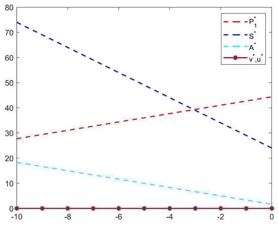
Figure 1.
Effect of on , and .
- (ii)
- Effect of on , and . Let , and .
Figure 2 shows that , and are positively correlated because a decrease in indicates a decrease in pollution; that is, the enterprise protects the environment by reducing its output. At this time, the local regulator encourages the enterprise by reducing product taxes. and are negatively correlated because a decrease in leads to a decrease in the enterprise’s output. To make more profits, the enterprise will increase the price of its products. and are not related to .
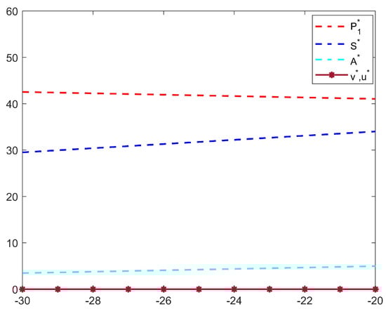
Figure 2.
Effect of on , and .
- (iii)
- Effect of on , and . Let , and .
Figure 3 shows that and are negatively correlated because a decrease in indicates that the enterprise’s production technology level is low. The environmental pollution caused by the production of the product increases. To protect the environment, the enterprise will invest more to improve its production technology level . , and are not related.
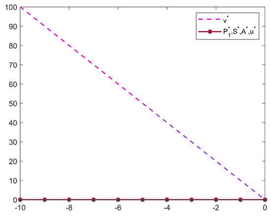
Figure 3.
Effect of on , and .
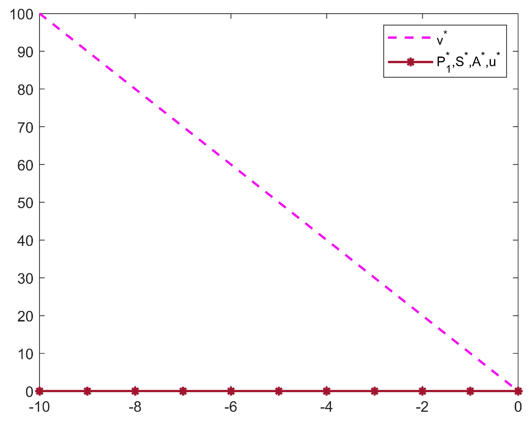
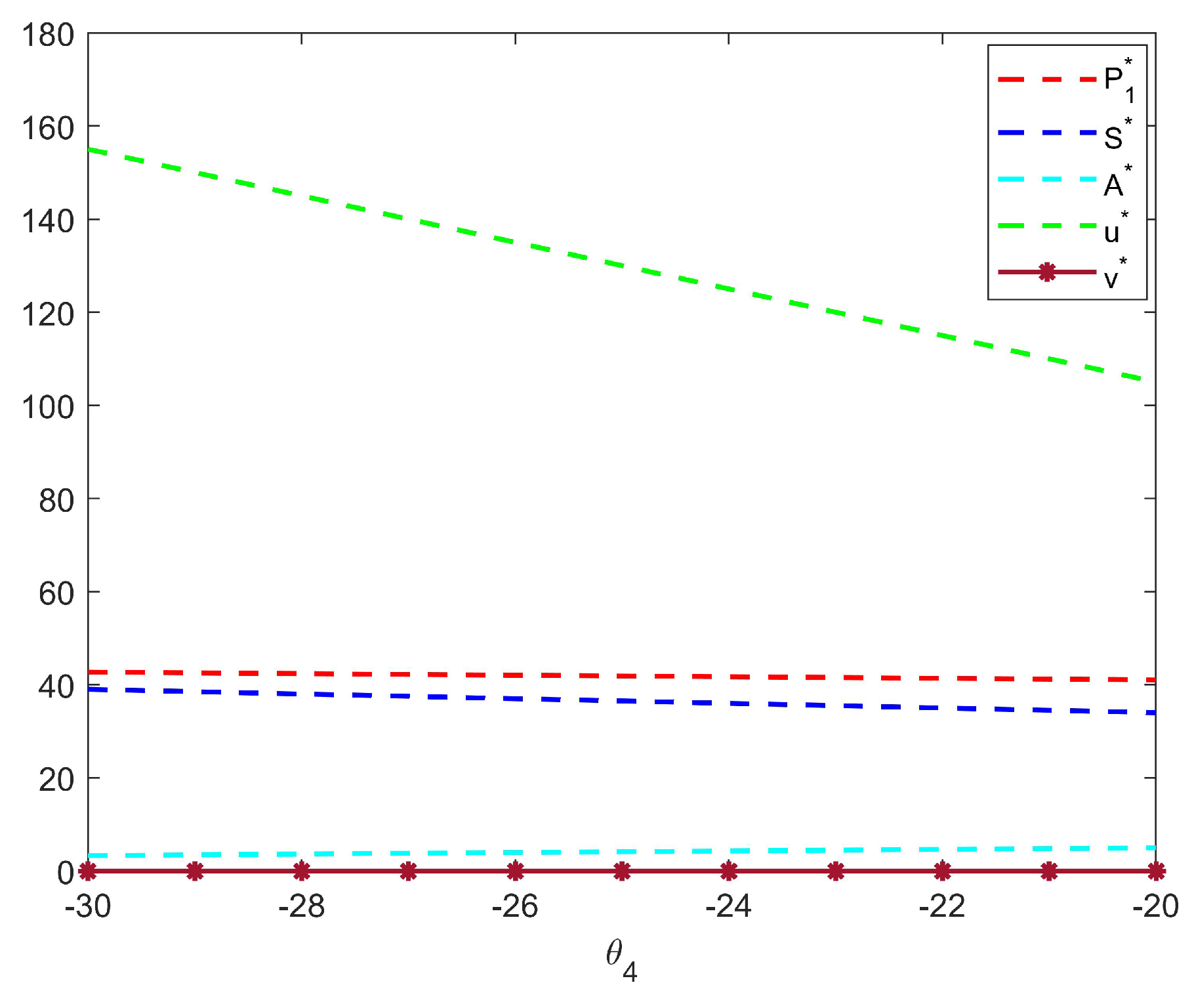
- (iiii)
- Effect of on , and . Let , and .
Figure 4 shows that and are positively correlated because a decrease in indicates that environmental protection is taken very seriously by the local regulator and penalties have been increased. The enterprise chooses to reduce its output. , and are negatively correlated because the decrease in shows a greater emphasis on environmental protection and increased penalties imposed by the local regulator, that is, a higher product tax levied by the local regulator. In this case, to obtain large profits, the enterprise reduces the output and increases the price of the products, leading to an increase in the local air pollution intensity. is not related to .
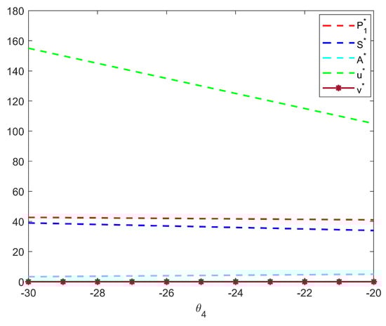
Figure 4.
Effect of on , and .
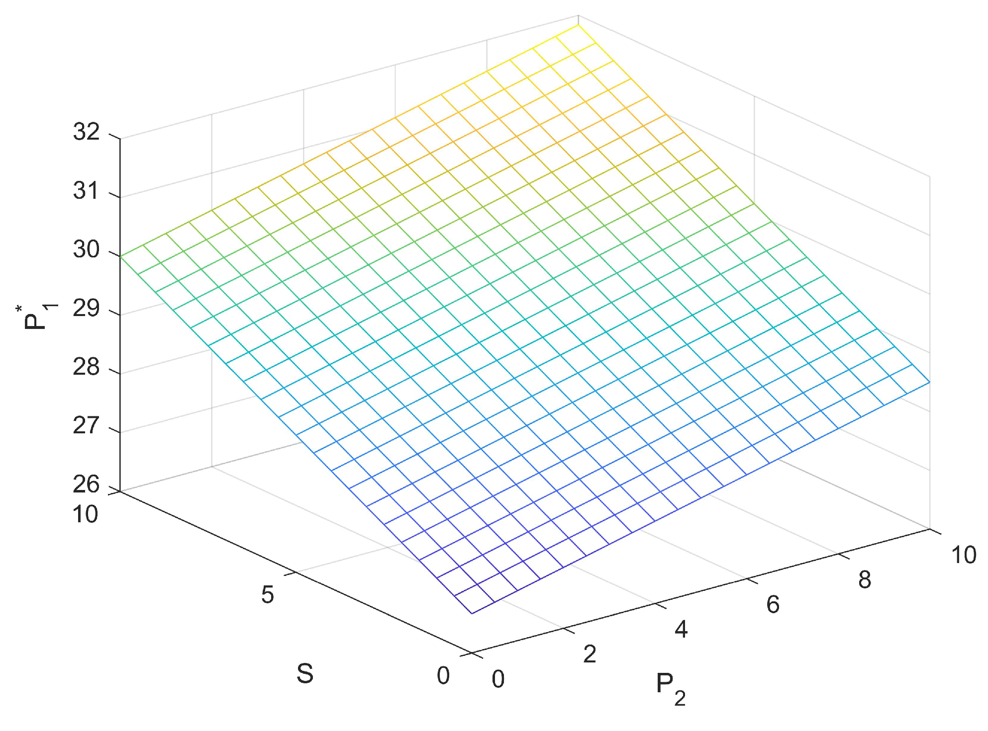
Next, this section analyzes the effects of reference prices and product taxes on the price of the enterprise’s products and the effect of social welfare benefits on environmental protection by the local regulator.
Figure 5 shows that the selling price of the enterprise’s products increases with the increase in the competing enterprise’s selling price and product tax. When the competing enterprise raises the price and the local regulator raises the product tax, the enterprise inevitably pays higher taxes if it continues to expand its output and to use the approach of small profits but quick turnover. The enterprise chooses to raise its price by producing fewer products to obtain more profits. Therefore, the increase in the product tax by the local regulator benefits local air protection.
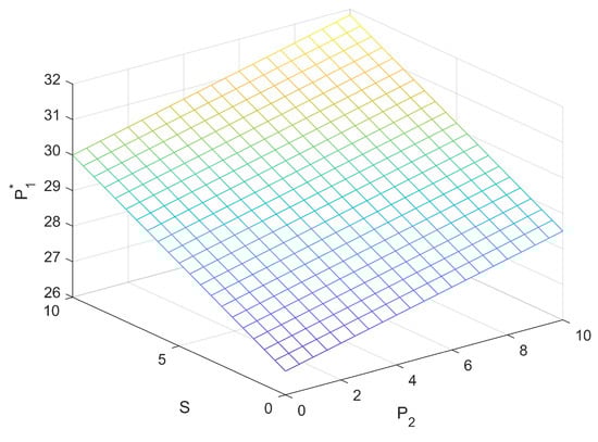
Figure 5.
Effect of and S on .
Tax on products is an essential variable that affects enterprises’ decisions. If the product tax is low, the enterprise will take the approach of small profits but quick turnover, which means that atmospheric contamination will increase. Therefore, the local regulator can increase the product tax to make it more costly for companies to increase production, further protecting the local atmosphere.
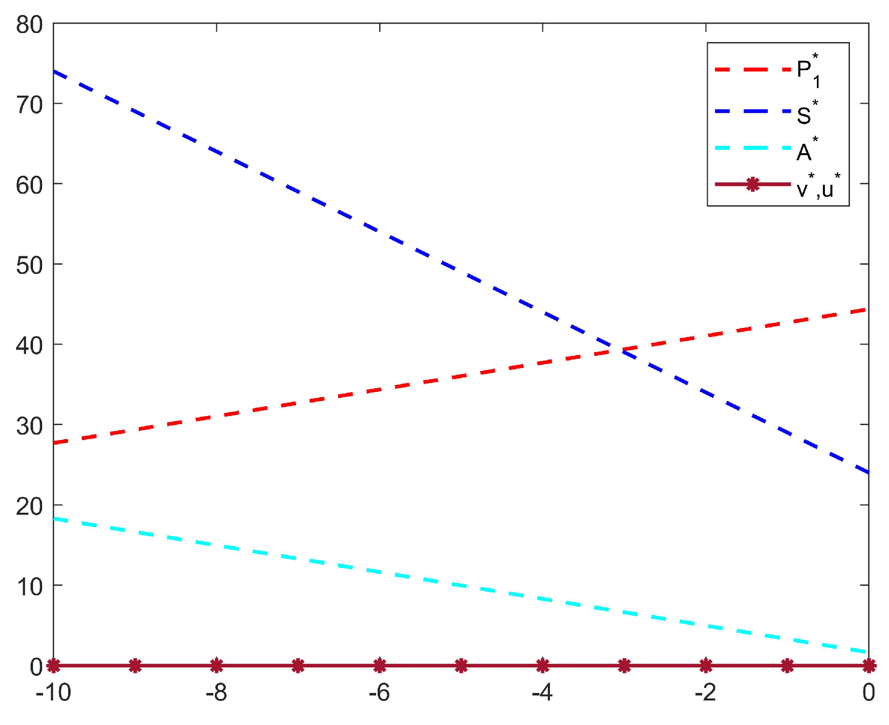
Figure 6 shows that by introducing social welfare benefits into the local regulator’s payoff function, the local regulator increases its efforts to protect the local air environment. This is because introducing a payoff function for social welfare gains helps balance the relationship between economic development and environmental protection. The local regulator usually needs to consider the community’s overall well-being, not just the short-term benefits of the economy at the expense of the environment. By considering social welfare, regulators can better weigh the potential environmental impacts of economic activities.
Figure 6.
Effect of on .
7. Conclusions
The establishment of a scientific ecological compensation mechanism is crucial to the protection of the environment. Although many research results have been achieved from the study of ecological compensation, most related research has focused on rivers and other areas, and only a few studies have been conducted on the air environment. Therefore, studying the ecological compensation mechanism of the air environment by using differential games is essential. To inform the public about air quality, China utilizes the AQI as a measure of air quality. Air pollution control can considerably improve residents’ living environment and provide social welfare benefits. Therefore, this study introduces the AQI and social welfare benefits and establishes a differential game model of the Stackelberg ecological compensation mechanism for air pollution between the local regulator and an enterprise with a competitor. The optimal dynamic strategies of the local regulator and the enterprise with a competitor are determined using the Pontryagin maximum principle, and the evolution of the shadow price is analyzed with the method of backward differential equations. Then, the effects of the shadow price on the decision-making variables of the local regulator and the enterprise and the effects of the social welfare benefits on the local AQI and the environmental protection efforts of the local regulator are analyzed through numerical simulation. The results show that introducing social welfare benefits enhances the local regulator’s efforts to protect the air environment and helps improve local air quality. From an ecological perspective, this study explores how a balance between the sustainable development of the local economy and the effective protection of the air environment can be achieved and how the profits of local enterprises can be maximized via the air pollution ecological compensation mechanism. The results of this study provide a theoretical basis for the formulation of effective ecological compensation policies for air pollution.
Author Contributions
Y.Y.: methodology; E.L. and Z.H. (Zuopeng Hu): writing—review and editing; S.X. and Z.H. (Zhijun Hu): funding acquisition. All authors have read and agreed to the published version of the manuscript.
Funding
This work was supported by the National Natural Science Foundation of China (Grant No. 71961003, Grant No. 72361007).
Institutional Review Board Statement
Not applicable.
Informed Consent Statement
Not applicable.
Data Availability Statement
Data sharing is not applicable to this paper, as no data sets were generated or analyzed during the current study.
Conflicts of Interest
The authors declare that they have no known competing financial interests or personal relationships that could have appeared to influence the work reported in this paper.
References
- Kilgour, D.M.; Okada, N.; Nishikori, A. Load control regulation of water pollution: An analysis using game theory. J. Environ. Manag. 1988, 27, 179–194. [Google Scholar]
- Petrosjan, L.; Zaccour, G. Time-consistent Shapley value allocation of pollution cost reduction. J. Econ. Dyn. Control 2003, 27, 381–398. [Google Scholar]
- Chang, S.; Qin, W.; Wang, X. Dynamic optimal strategies in transboundary pollution game under learning by doing. Phys. A Stat. Mech. Its Appl. 2018, 490, 139–147. [Google Scholar] [CrossRef]
- Gao, X.; Shen, J.; He, W.; Sun, F.; Zhang, Z.; Guo, W.; Zhang, X.; Kong, Y. An evolutionary game analysis of governments’ decision-making behaviors and factors influencing watershed ecological compensation in China. J. Environ. Manag. 2019, 251, 109592. [Google Scholar] [CrossRef] [PubMed]
- Isaacs, R. Differential Games; John Wiley and Sons: New York, NY, USA, 1965. [Google Scholar]
- Long, N.V. Pollution control: A differential game approach. Ann. Oper. Res. 1992, 37, 283–296. [Google Scholar] [CrossRef]
- Ploeg, F.; Zeeuw, A. International Aspects of Pollution Control. Environ. Resour. Econ. 1992, 2, 117–139. [Google Scholar] [CrossRef]
- Yeung, D. Dynamically Consistent Cooperative Solution in a Differential Game of Transboundary Industrial Pollution. J. Optim. Theory Appl. 2007, 134, 143–160. [Google Scholar] [CrossRef]
- Yeung, D.; Petrosjan, L. A cooperative stochastic differential game of transboundary industrial pollution. Automatica 2008, 44, 1532–1544. [Google Scholar] [CrossRef]
- Jiang, K.; Merrill, R.; You, D.; Pan, P.; Li, Z. Optimal control for transboundary pollution under ecological compensation: A stochastic differential game approach. J. Clean. Prod. 2019, 241, 118391. [Google Scholar] [CrossRef]
- Jiang, K.; You, D.; Li, Z.; Shi, S. A differential game approach to dynamic optimal control strategies for watershed pollution across regional boundaries under eco-compensation criterion. Ecol. Indic. 2019, 105, 229–241. [Google Scholar] [CrossRef]
- Wei, C.; Luo, C. A differential game design of watershed pollution management under ecological compensation criterion. J. Clean. Prod. 2020, 274, 122320. [Google Scholar] [CrossRef]
- Yi, Y.; Wei, Z.; Fu, C. A Differential Game of Transboundary Pollution Control and Ecological Compensation in a River Basin. Complexity 2020, 2020, 6750805. [Google Scholar] [CrossRef]
- Chen, Z.; Meng, Q.; Wang, H.; Xu, R.; Yi, Y.; Zhang, Y. Dynamic Optimal Control Differential Game of Ecological Compensation for Multipollutant Transboundary Pollution. Complexity 2021, 2021, 5530971. [Google Scholar] [CrossRef]
- Ding, J.; Chen, L.; Deng, M.; Chen, J. A differential game for basin ecological compensation mechanism based on cross-regional government-enterprise cooperation. J. Clean. Prod. 2022, 362, 132335. [Google Scholar] [CrossRef]
- Teng, M.; Zhao, M.; Han, C.; Liu, P. Research on mechanisms to incentivize corporate environmental responsibility based on a differential game approach. Environ. Sci. Pollut. Res. 2022, 29, 57997–58010. [Google Scholar] [CrossRef]
- Yi, Y.; Ding, C.; Fu, C.; Li, Y. Transboundary watershed pollution control and product market competition with ecological compensation and emission tax: A dynamic analysis. Environ. Sci. Pollut. Res. 2022, 29, 41037–41052. [Google Scholar] [CrossRef]
- Huang, X.; He, P.; Zhang, W. A cooperative differential game of transboundary industrial pollution between two regions. J. Clean. Prod. 2016, 120, 43–52. [Google Scholar] [CrossRef]
- Sun, H.; Gao, G.; Li, Z. Research on the cooperative mechanism of government and enterprise for basin ecological compensation based on differential game. PLoS ONE 2021, 16, e0254411. [Google Scholar] [CrossRef] [PubMed]
- Deng, M.; Chen, J. A market sharing mechanism for watershed ecological compensation. Water Supply 2022, 22, 7565–7575. [Google Scholar] [CrossRef]
- Wang, Y.; Wu, X.; Shen, J.; Chi, C.; Gao, X. Analysis on Decision-Making Changes of Multilevel Governments and Influencing Factors in Watershed Ecological Compensation. Complexity 2021, 2021, 6860754. [Google Scholar] [CrossRef]
- Fibich, G.; Gavious, A.; Lowengart, O. Explicit Solutions of Optimization Models and Differential Games with Nonsmooth (Asymmetric) Reference-Price Effects. Oper. Res. 2003, 51, 721–734. [Google Scholar] [CrossRef]
- Stackelberg, H.V. Market Structure and Equilibrium; Spinger: Berlin/Heidelberg, Germany, 1934. [Google Scholar]
- Basar, T.; Zaccour, G. Handbook of Dynamic Game Theory; Springer: Berlin/Heidelberg, Germany, 2018. [Google Scholar] [CrossRef]
Disclaimer/Publisher’s Note: The statements, opinions and data contained in all publications are solely those of the individual author(s) and contributor(s) and not of MDPI and/or the editor(s). MDPI and/or the editor(s) disclaim responsibility for any injury to people or property resulting from any ideas, methods, instructions or products referred to in the content. |
© 2024 by the authors. Licensee MDPI, Basel, Switzerland. This article is an open access article distributed under the terms and conditions of the Creative Commons Attribution (CC BY) license (https://creativecommons.org/licenses/by/4.0/).