Abstract
Carbon trading risk management and policy making require accurate forecasting of carbon trading prices. Based on the sample of China’s carbon emission trading pilot market, this paper firstly uses the Augmented Dickey–Fuller test and Autoregressive conditional heteroscedasticity model to test the stationarity and autocorrelation of carbon trading price returns, uses the Generalized Autoregressive Conditional Heteroscedasticity family model to analyze the persistence, risk and asymmetry of carbon trading price return fluctuations, and then proposes a hybrid prediction model neural network (generalized autoregressive conditional heteroscedasticity–long short-term memory network) due to the shortcomings of GARCH models in carbon price fluctuation analysis and prediction. The model is used to predict the carbon trading price. The results show that the carbon trading pilots have different degrees of volatility aggregation characteristics and the volatility persistence is long, among which only the Shanghai and Beijing carbon trading markets have risk premiums. The other pilot returns have no correlation with risks, and the fluctuations of carbon trading prices and returns are asymmetrical. The prediction results of different models show that the root mean square error (RMSE) of Hubei, Shenzhen and Shanghai carbon trading pilots based on the GARCH-LSTM model is significantly lower than that of the single GARCH model, and the RMSE values are reduced by 0.0006, 0.2993 and 0.0151, respectively. The RMSE in the three pilot markets improved by 0.0007, 0.3011 and 0.0157, respectively, compared to the standalone LSTM model. At the same time, compared with the single model, the GARCH-LSTM model significantly increased the R^2 value in Hubei (0.2000), Shenzhen (0.7607), Shanghai (0.0542) and Beijing (0.0595). Therefore, compared with other models, the GARCH-LSTM model can significantly improve the prediction accuracy of carbon price and provide a new idea for scientifically predicting the fluctuation of financial time series such as carbon price.
1. Introduction
As the global ecological environment deteriorates and environmental problems intensify, countries around the world have recognized the serious hazards caused by environmental issues. In order to effectively reduce greenhouse gas emissions and mitigate environmental problems, carbon emissions trading markets have emerged. According to ICAP data, the global carbon trading market will cover 17% of global greenhouse gas emissions in 2023, and China’s carbon market is the largest in the global carbon market in terms of covered carbon emissions. The establishment of a carbon emission trading market is the most effective way for China to effectively achieve climate governance and green and high-quality development. (Jia and Lin, 2022) [1]. During the operation of the carbon market, accurate forecasting of carbon trading prices is essential for carbon market participants to compete. At the same time, the government and policy makers should conduct timely supervision based on the future direction of carbon trading prices when market trading risks may occur and regulate the behavior of participants, ensuring the long-term stability and orderly development of the carbon emissions trading market.
As a new financial market, China has a large potential carbon trading market but still remains immature. It is shown that the fluctuation of carbon price is unstable, and the fluctuation of different markets is very different. The carbon trading prices exhibit volatility and complexity, posing certain obstacles to resource allocation and the improvement of market price regulation mechanisms. However, most domestic scholars have used ARCH family models and recurrent neural network models for the analysis and prediction of carbon prices. The GARCH model only considers the volatility of variance, while recurrent neural network models face the problem of exploding or vanishing gradients. Therefore, the methods currently used in domestic research cannot achieve good predictions. Thus, accurately identifying the volatility characteristics of carbon prices and reasonably predicting them have become the top priority of current research on carbon price prediction.
With the increasing attention on the rationality of carbon trading prices, volatility characteristics and carbon price prediction have attracted more and more attention from scholars (Böhringer et al., 2006) [2]. As for the volatility characteristics of carbon emission trading prices, the EU carbon emission trading market has been established for a longer time and the trading system is more complete. Mansanet M et al. (2007) found that the carbon emission price in the EU carbon emission trading market is similar to the stock price, showing asymmetric and continuous volatility [3]. Chevallier (2011) believes that the future price returns of EUA, in addition to asymmetrical features, also exhibit significant volatility clustering and long-term memory characteristics (Cong et al., 2017) [4,5]. Volatility concentration shows that the price yield of the carbon trading market fluctuates around the mean value. If the yield rate is small in a certain period, the yield rate will continue to decrease in the next period. Or if the rate of return is large in a certain period of time, the rate of return will continue to increase over the next period of time, and there is volatility accumulation. The volatility accumulation of carbon price and market shocks over time have a lasting impact on future prices, and the recovery speed is relatively slow. Zhang Yuejun et al. (2011) analyzed the carbon price characteristics of the EU carbon market through the GARCH model, VAR model and mean reversion method and found that the fluctuation of carbon quota price returns did not follow the mean reversion process [6]. With the development of China’s carbon emission trading pilot, scholars have gradually paid attention to the fluctuation rule of China’s carbon emission trading price. Lv Yongbin et al. (2015) and Zhang Jie et al. (2018) believe that carbon price changes over time have obvious clustering characteristics [7,8], and Lv jingye et al. (2019) believe that China’s carbon price yield has a strong long-term memory [9]. Zhang Jing and Cui Yinglin (2021) found that due to investors’ different interpretations of the official launch of the carbon trading market, there would be abnormal fluctuations in carbon price returns, resulting in abnormal fluctuations in carbon price returns [10].
In terms of carbon price prediction, there are significant differences in the carbon price of the same carbon market under different prediction models, and model selection is crucial to accurately predict carbon price (Kainuma, 1999) [11]. Based on the different types of prediction models, scholars have mainly discussed the prediction of China’s carbon trading price from three aspects: first, the prediction of carbon price by using traditional econometric methods; second, prediction based on single models such as neural networks and machine learning and third, the prediction of carbon market price by using a combination model of the above two methods.
(1) For econometric methods, Li et al. (2015) used empirical mode decomposition, generalized autoregressive conditional heteroscedasticity and a CGE model to predict China’s carbon price based on historical carbon price data [12]. Lv Jingye et al. (2019) used an ARIMA model to predict the future price of the EU carbon financial market [9]. Zhang Chen et al. (2016) and Zhao Lingdi et al. (2019) built a multi-frequency combination prediction model to study the change trend of carbon trading prices [13,14]. Wei Yu et al. (2022) considered the key factors affecting carbon prices and used various classical prediction models and dynamic model selection and dynamic model average methods to forecast carbon prices in typical regions of China [15]. Liu et al. (2021) and Gong Weifeng et al. (2022) made predictions based on the traditional econometric GARCH model [16,17]. However, the GARCH model can only solve the heteroscedasticity phenomenon that carbon price series fluctuate more in the market fluctuation period and less in the market stability period and cannot describe the multifractal characteristics.
(2) Aimed at single model methods such as neural networks and machine learning, Zhang Chen et al. (2016) used the pole symmetric mode decomposition method, nonlinear auto regression, a neural network and support vector machine to build a carbon price multi-frequency combination prediction model for carbon market price prediction [13]. Yun et al. (2020) built a new carbon price prediction method based on an NAGARCHSK-LSTM model, considering the special characteristics of carbon price asymmetry, extreme shock sensitivity and time-varying fluctuations [18]. Zhao et al. (2023) used the Adam algorithm to optimize the long- and short-term memory method to predict CTP points. In addition, scholars generally regard the LSTM neural network model (Hochreiter and Schmidhuber, 1997) as the current mainstream machine prediction model [19,20]. With the characteristics of time series selection memory and interaction, it can effectively solve the problem of unstable carbon price (Dey et al., 2021; Marzouk et al., 2021; Chen et al., 2021, Yang et al., 2022) [21,22,23,24]. However, Jian Wei et al. (2019) believe that although econometric models such as GARCH can effectively capture the fluctuations in carbon prices, they cannot accurately adapt to the nonlinear and non-stationary characteristics of carbon prices [25]. The use of these models alone has certain prediction limitations, which do not fully consider the influence of time series features and the special redundancy problem in data on trend prediction, resulting in weak prediction ability (Wang Xiaolei et al., 2021) [26].
(3) Aimed at the combined prediction method of econometrics and intelligent machine learning, in order to better improve the accuracy of carbon price prediction, scholars are gradually adopting mixed models (Hao et al., 2020; Adekoya, 2021) [27,28]. Some scholars have proposed an ELM-AWOA model (Sun and Zhang, 2018) [29], CPN-ELM model (Xu et al., 2020) [30] and MOEMD-ELM hybrid model (Huang and He, 2020) [31] LSSVR, NARNN and Holts exponential smoothing model (Zhu et al., 2019) [32] and LSSVR-PSO model (Jianwei et al., 2021) [33], and all demonstrate that combined models can predict prices more accurately than single forecasting models. For example, Yang et al. (2020) used the LSTM-IWOA model to predict the carbon trading prices of the Beijing, Fujian and Shanghai carbon markets [34]. The research results show that the optimized LSTM model has higher prediction accuracy, and its error is significantly lower than that of BP and ELM models. In addition, combined models such as LSTM-BP and LSTM-IWOA do not fully consider the time series characteristics of the data and the influence of feature redundancy on the trend prediction in trend forecasting. Hang et al. (2021) proposed a new disintegration–integration paradigm VMD-GARCH/LSTM-LSTM model for carbon price prediction, in which the LSTM network predicts the low-frequency sub-model and GARCH model predicts the high-frequency sub-model, effectively reducing the prediction error [35]. Kakade et al. (2023) proposed to combine LSTM and Bi LSTM models with GARCH-type models and found that the BI-LSTM model and GARCH-type model had the best performance and the lowest values of the two loss functions. Bi LSTM (bidirectional long short-term memory) is the process of making any neural network have sequential information in both the backward (future-to-past) or forward (past-to-future) directions [36]. BP and LSTM are both neural network methods, and LSTM is superior to the BP network method in terms of time series and sequence data processing and analysis. In summary, GARCH-LSTM is used to incorporate time series and other features into the model, which better avoids the disadvantages of the above models and solves the influence of feature term redundancy on trend prediction. At the same time, different from the GARCH-LSTM model used in other reports, the GARCH family model coefficients containing sequence information are added to the input layer of the LSTM model, and the LSTM model can predict the data with long feature intervals and delay to learn the sequence features. The accuracy of the prediction results is thus improved. In addition, there are no studies using the GARCH-LSTM model to explore the agglomeration, asymmetry and risk premium of carbon price fluctuations and to predict carbon price and its future fluctuations. Therefore, this article has a certain originality.
From the above literature review, it can be seen that some research studies have been carried out on the characteristics and prediction of carbon trading price fluctuations in different countries and regions, but there are still areas for improvement. On the one hand, the existing studies mainly use historical carbon price data to construct econometric models or intelligent machine learning models and then predict the current carbon price. Also, the key factors that have a greater impact on carbon price fluctuations, such as the energy market, financial market, international carbon market and natural environment are not considered enough. It is difficult to effectively capture the time-varying high-order moment characteristics of the carbon price. On the other hand, the accuracy of existing intelligent machine learning methods for carbon price prediction is usually higher than that of traditional econometric model methods, but it needs to be further improved. The GARCH-LSTM combination model combined with the traditional econometric model is a relatively new intelligent machine learning prediction method which can accurately extract the price series feature information. The deep learning GARCH family model has its own characteristics and uses the advantages of the LSTM model to predict the data with long feature intervals and long delay to learn the sequence features, and the prediction performance is better than that of the traditional neural network. Therefore, this paper uses this model to predict the carbon price.
From the above point of view, there are two shortcomings in the existing literature on the study of carbon price fluctuation characteristics and prediction. First of all, there are limited comprehensive research studies on the volatility characteristics of carbon prices in multiple carbon trading pilots in China and the existing studies lack of testing of the volatility characteristics of carbon prices, resulting in the neglect of the comprehensive utilization of the characteristics of carbon price volatility such as agglomeration, risk premium and asymmetry.
Second, this paper’s emphasis is on the construction of a price volatility prediction model based on the GARCH model. Indeed, a long-term memory neural network improves the accuracy of carbon price prediction. However, the contribution of long-term neural networks to single models and hybrid prediction models in the field of carbon price research needs to be further explored. For these purposes, this article attempts to answer three questions: how to accurately identify the characteristics of price fluctuations in carbon trading markets, whether deep machine learning methods can help improve forecasting and how to combine traditional econometric methods with deep machine learning methods. The main work and contributions of this paper are summarized as follows:
(1) The ADF unit root test and ARCH effect test are used to test carbon price volatility in the Chinese carbon market, making the test results on the sustainability, risk and asymmetry characteristics of carbon price volatility more convincing. Furthermore, we look for reasons for these erratic fluctuations in carbon prices to help people understand how carbon prices fluctuate.
(2) This article answers the question of whether deep learning methods can improve the accuracy of carbon market price forecasts in China. In addition, the effect of different prediction methods on improving the prediction accuracy is quantitatively evaluated.
(3) A hybrid prediction model containing the GARCH-class model and LSTM model, named the GARCH-LSTM model, is established to forecast the carbon price in China’s carbon market.
2. Methodology
The volatility of financial time series has the characteristics of time variability, aggregation and long-term memory. The generalized autoregressive conditional heteroscedasticity (GARCH) model can better solve the heteroscedasticity phenomenon of carbon trading price series in the market volatility period, but in the market stability period. In this paper, the GARCH family model is constructed to explore the volatility characteristics of China’s carbon trading price yield. The ARCH model considers the volatility of variance, and the GARCH-LSTM neural network model is added to the GARCH model to construct the GARCH-LSTM combined model, which provides a new way to study the volatility of financial time series.
2.1. GARCH Model (Generalized Autoregressive Conditional Heteroscedasticity)
Bollerslev (1986) proposed the GARCH model, which can not only detect the persistence of volatility but also reflect long-term memory and nonlinear features of volatility [37]. The equation for the GARCH model is as follows:
In Equation (2), m represents the lag order of the autoregressive term, and q represents the lag order of the squared residual term. Both m and q are greater than or equal to zero (m ≥ 0, q ≥ 0). The parameters , are the coefficients of the ARCH and GARCH terms, respectively, and they must be greater than zero ( (i = 1, 2, …… m), (j = 1, 2, …… p)). The term quantifies the impact of external shocks on the persistence of volatility. The GARCH model has strong explanatory power for the volatility of time series data and can enhance the accuracy of studying the volatility characteristics of asset prices.
2.2. GARCH-M Model (GARCH in MEAN)
In order to reflect the risk premium in the financial market, Engle et al. (1987) proposed to add variance to the mean value equation to analyze the relationship between price return and risk in the financial market. The GARCH-M model extends the GARCH model by incorporating lagged terms into the variance equation of the ARCH model [38]. The variance equation is as follows:
In Equation (3), represents the risk coefficient, which represents the financial market risk, and denotes the risk premium. When , there is a positive correlation between return and risk in the financial market. On the other hand, when , there is an inverse correlation between returns and risk in the financial market.
The development level of China’s carbon trading market is not high enough, and the impact of risk on the price and return of each carbon trading market is also different. In order to discover the correlation between risk and return in the carbon trading market and whether there is a risk premium, it is more appropriate to choose the GARCH-M model to test the impact of risk on the carbon trading price.
2.3. TGARCH Model (Threshold GARCH)
When the financial time series is subjected to the same degree of positive and negative shocks, the impact is different. Generally, most of the positive shocks have a small impact on the financial time series, while the negative shocks have a greater “power” and generally have a more obvious impact on the financial time series. The asymmetry of this wave cannot be explained by the GARCH model due to its own limitations. Therefore, in order to further and better describe this wave asymmetry, Glosten et al. (1993) added a dummy variable to the GARCH variance model, set a threshold to detect the impact of bad news and good news on asset price fluctuations, and proposed an asymmetric “threshold GARCH model”, briefly referred to as the TGARCH model [39]. The equation for the TGARCH model is as follows:
In the equation, k represents the number of thresholds. When , , which means that the economic situation improves or good news occurs. On the other hand, when , , indicating the occurrence of bad news. When the parameter γ > 0, bad news has a greater impact on volatility. Conversely, when the parameter γ < 0, the impact of good news is greater than that of bad news.
Different carbon trading pilots in China have different levels of development and different responses to positive and negative impacts brought by external news. In order to test whether there are differences in the impact of good news and bad news on the volatility of carbon trading price yield, it is more appropriate to choose the TGARCH model to test the asymmetric characteristics of carbon trading prices.
2.4. LSTM Neural Network (Long Short-Term Memory Network)
LSTM is a special type of Recurrent Neural Network (RNN) that effectively addresses the issue of handling long sequences of data and obtaining long-distance information, which traditional RNNs struggle with due to problems like vanishing or exploding gradients. It can be used to predict price data with long feature intervals and long delays.
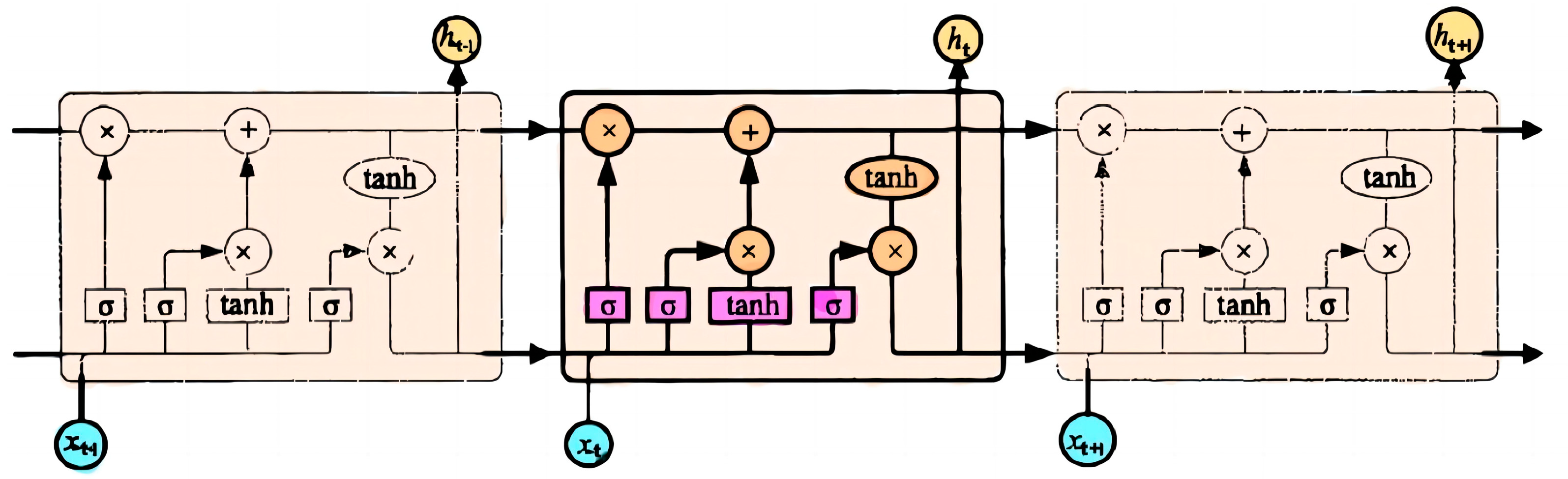
The concept behind LSTM is to selectively remember information by employing a memory cell. The LSTM neural network consists of an input gate, an output gate, a forget gate and a memory cell. The horizontal line inside the box is referred to as the cell state, which controls the information flow to the next time step. The forget gate, as shown in Equation (6), plays a role in determining whether certain information should be forgotten from long-term memory based on both the short-term memory information and the current input. It is controlled using a sigmoid function, taking into account the previous time step output and the current input to produce a forget factor (ranging between 0 and 1). The σ symbol represents the sigmoid function, and denotes the weight values, while represents the intercept term.
The input gate, determined by the sigmoid function, in this process is represented by Equations (7)–(9). In these equations, takes values of 0 or 1, and tanh denotes the hyperbolic tangent activation function, represents the cell value state, represents the stored input quantity and represents the new cell state value.
Finally, the output gate comes into play. First, the sigmoid layer decides which part of the updated cell state is to be stored as input for the next time step. Then, the tanh layer maps the values to the range of −1 to 1. The output from the sigmoid and the output from the tanh are multiplied element-wise to obtain the model’s output, as shown in Equations (10) and (11).
LSTM is composed of memory blocks rather than neurons. Through a storage unit and three control gates, LSTM can select and learn data well and form memory for historical information with long time intervals. With the increase in information, the LSTM model can effectively learn the features required to predict the realized price fluctuations, so that the key information in the price data can be effectively updated and transmitted and the market price fluctuation rule of carbon trading price can be better captured, thus improving the prediction accuracy of the carbon trading market price. Figure 1 shows the LSTM logical structure.
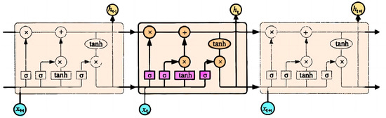
Figure 1.
Logical structure of LSTM neural network.
2.5. GARCH-LSTM
In terms of predictive data accuracy, deep learning and GARCH family models have their own characteristics. The GARCH family model has the ability to mine the economic characteristics of time series, and deep learning also has its own characteristics in predicting problems and solving complex models, which uses fewer assumptions and fewer modeling constraints and can optimize the learning characteristics; so, this paper adds the GARCH family model coefficients containing sequence information to the input layer of the LSTM model, where the input layer is the parameter and estimates of the GARCH model. The output layer is the true value of the carbon trading price yield. Then, the LSTM model can predict data with long feature intervals and long delay by learning these features of the input variables so as to improve the prediction performance of the model.
3. Data
Since 2011, there have been a total of eight carbon emissions trading pilot markets established in China. Due to differences in market demand, mechanisms and policies among these carbon markets, their levels of activity vary, leading to differences in trading volume, liquidity, turnover, product diversity and price volatility. As shown in Table 1, as of June 2023, the cumulative total trading volume of allowances in the Hubei carbon emission trading market was 372.742 million tons, with a total transaction volume of CNY 8,818,786,000, ranking first in the country in terms of transaction scale and market share. The cumulative total amount of allowances in the Chongqing carbon emission trading market was 29.228 million tons, and the total transaction volume was CNY 355.682 million, ranking last. Furthermore, the Fujian market, as a newly established pilot, has limited available transaction data. The Chongqing and Tianjin pilot markets have relatively short periods of effective operation, resulting in very limited daily trading activities. On the other hand, the other five pilot markets in Hubei, Shenzhen, Shanghai, Beijing and Guangdong were among the first established carbon emissions trading markets in China. They not only account for a combined 89.41% of the total trading volume and 92.63% of the total turnover but also exhibit typical characteristics in terms of the diversity of carbon emissions trading products and the liquidity of trading funds.

Table 1.
Trading situation of China’s carbon trading pilot market.
The data for this study were collected from the carbon emissions trading centers in five pilot markets: Hubei, Shenzhen, Shanghai, Beijing and Guangdong. The carbon emissions trading average prices from 8 May 2014 to 18 October 2022 were selected as the carbon trading prices for analysis, and the data were sourced from the Wind database. To obtain more stable quasi-noise time series, the method proposed by Zhang Jing and Cui Yinglin (2021) was adopted. Specifically, the natural logarithm was applied to the carbon trading prices in each pilot region, transforming the price series into a series of returns using the formula for continuous compound returns (Equation (12)).
In the above equation, represents the return at time t, and represents the carbon trading price at time t. The returns for each of the five carbon trading pilot markets, namely Hubei, Shenzhen, Shanghai, Beijing and Guangdong, are denoted as , , , , , respectively. The characteristics of the returns for these five carbon trading pilot markets were studied. For the analysis, the sample period was set from 8 May 2014 to 18 October 2022. The sample data were processed using Equation (12) to obtain the corresponding returns. Considering factors such as non-trading days, the dataset was further refined by removing zero and missing values after difference transformation, resulting in single-day carbon return rate time series data for the carbon trading pilot markets, with a sample size of 839. The first 500 data points were used as the training set for the GARCH-LSTM combined model, while the remaining 339 data points were used as the test set for the combined model.
4. Empirical Analysis
4.1. Time Series Variation of Carbon Trading Price Returns
On the one hand, due to differences in market demand and mechanisms, there are significant variations in carbon emissions prices among different markets. Beijing has relatively higher carbon prices, while Guangdong has the lowest. On the other hand, each carbon market responds differently to external shocks, leading to varying levels of price volatility. Shenzhen experiences the highest price fluctuations, while Hubei exhibits relatively smaller price fluctuations. However, the price volatility trends across all carbon trading markets are similar, with significant initial increases followed by gradual declines. Through continuous improvements in carbon market mechanisms and policies, the price fluctuations eventually stabilize.
Table 2 describes five coal trading lead markets using descriptive statistics and analyses the volatility of coal trading price returns based on basic statistical properties. From the results of Table 2, it is observed that the price returns of the five carbon trading markets fluctuate around the mean, with some observations showing large fluctuations and others showing smaller ones, forming clusters of high and low volatility, indicating significant volatility clustering phenomena. In terms of the mean price returns, the Hubei carbon trading pilot market fluctuates the most; the average value of the Hubei market tends to be zero and the standard deviation is the smallest in all markets, reflecting the relatively good stability of the trading price fluctuation in the Hubei market. The yield jump of the Shenzhen carbon trading market is obvious, and the continuity of yield is not strong, mainly because the lack of suspension days in the Shenzhen carbon emission trading market led to structural breakpoints.
Table 2.
Statistical description of price-return series of carbon trading markets in China.
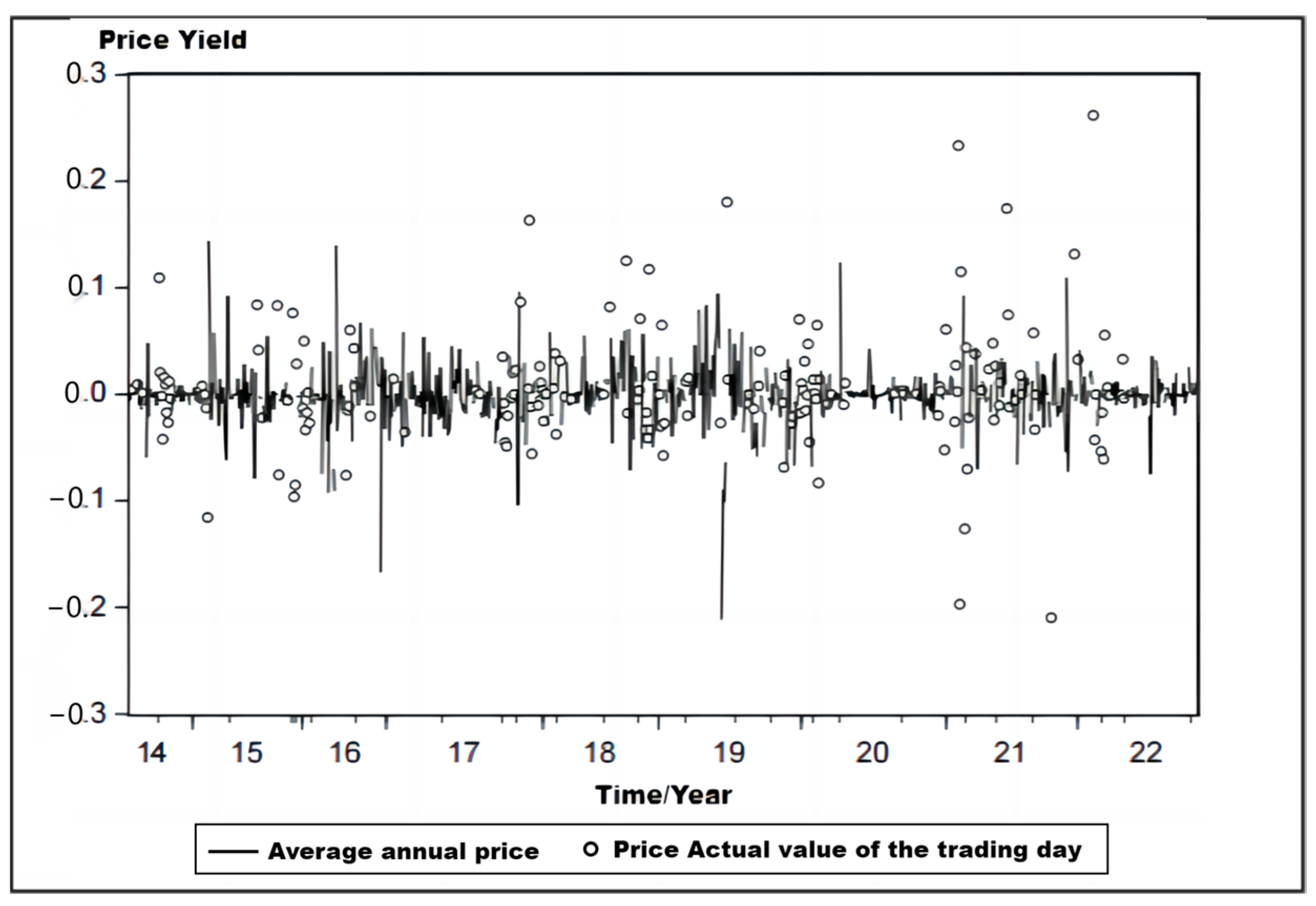
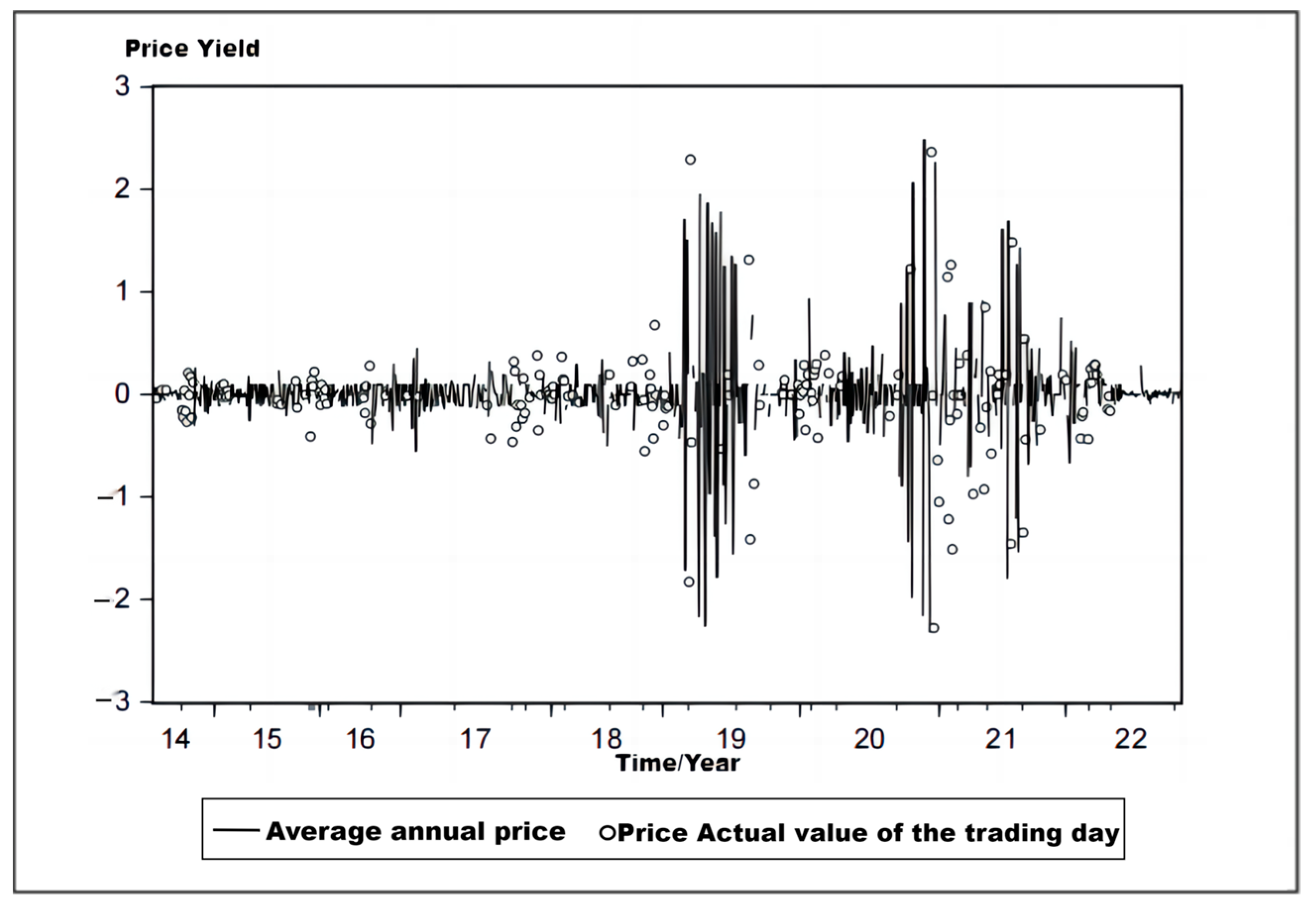
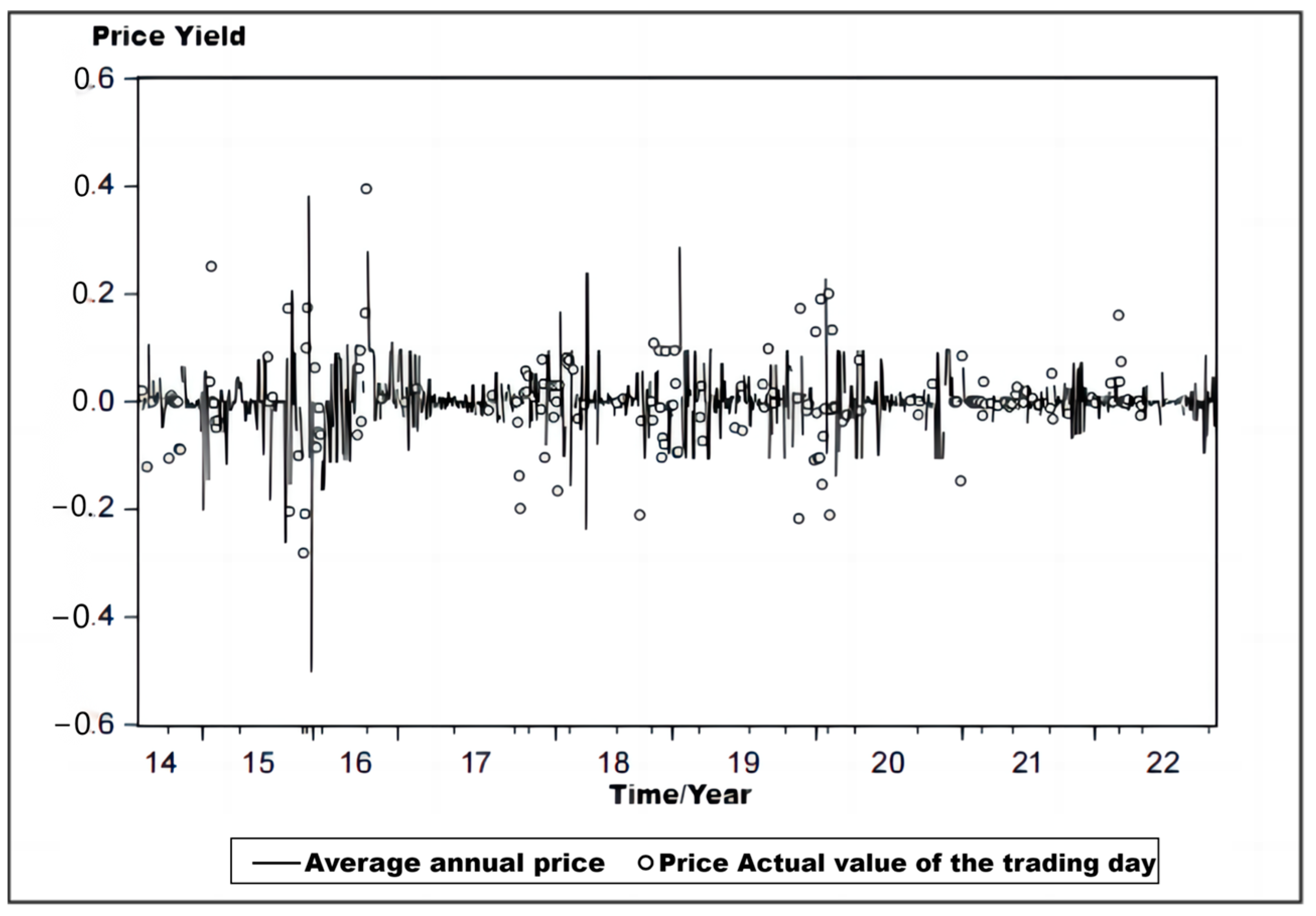
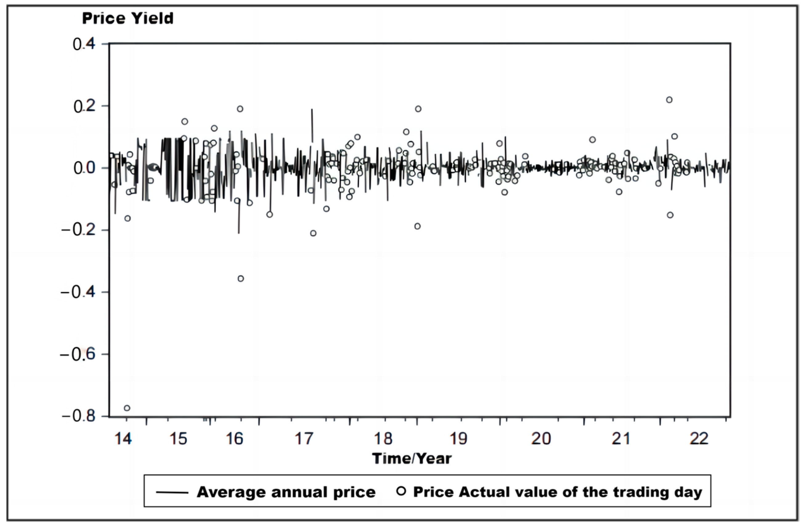
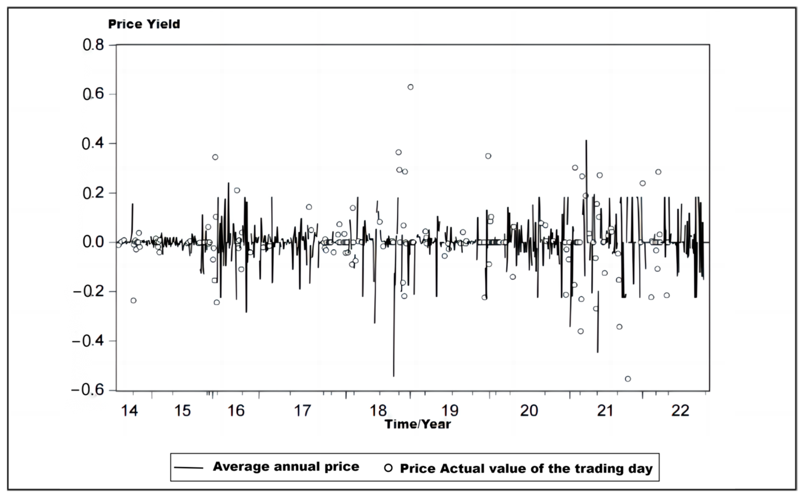
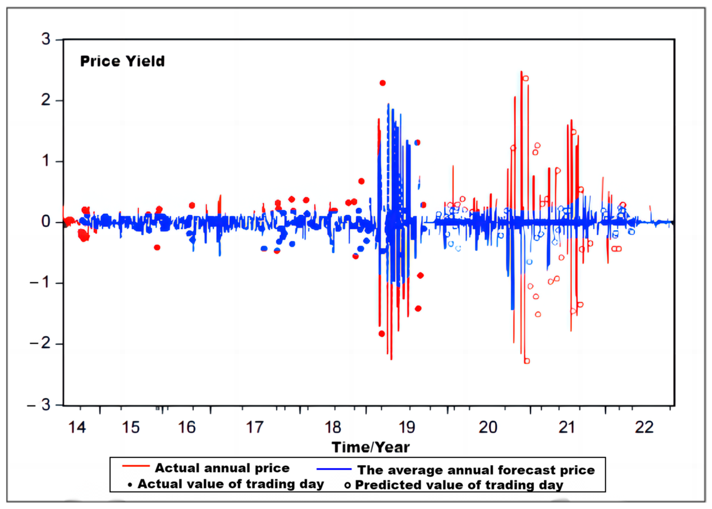
In addition, the maximum price yield is −2.321046 and the minimum price yield is 2.479478, indicating that its price–return rate fluctuates greatly. At the same time, there is also a clear temporal variation in the price–earnings ratio of the Beijing carbon pilot market due to the large number of trading days in Beijing. There is a certain lack of data, which is reflected in the Figure 2, Figure 3, Figure 4, Figure 5 and Figure 6, showing that there is a significant jump in the price–return rate, and the continuity is not strong. The pilot carbon trading market in Beijing has the lowest price–return ratio of the five pilot projects, with an average value of −0.000409 and a standard deviation of 0.092899, which also indicates that the price–return rate fluctuates greatly. Compared with the carbon emission market in Shenzhen, the standard deviation of the price–return ratio of the carbon emission market in Shanghai is 0.063511, the minimum value is −0.500775, the maximum value is 0.395313 and the difference between the maximum and minimum value is 0.896088, indicating that the prices and profit margins in the carbon emissions market are quite variable. The standard deviation of the price–return ratio of Guangdong carbon market is 0.056612, the minimum value is −0.774293, the maximum value is 0.220413 and the difference between the maximum and minimum values is 0.994706.
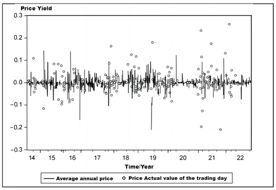
Figure 2.
Price yield fluctuation in Hubei carbon trading market.
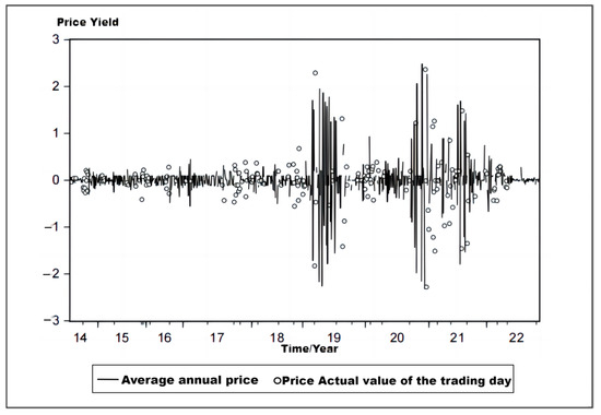
Figure 3.
Price yield fluctuation in Shenzhen carbon trading market.
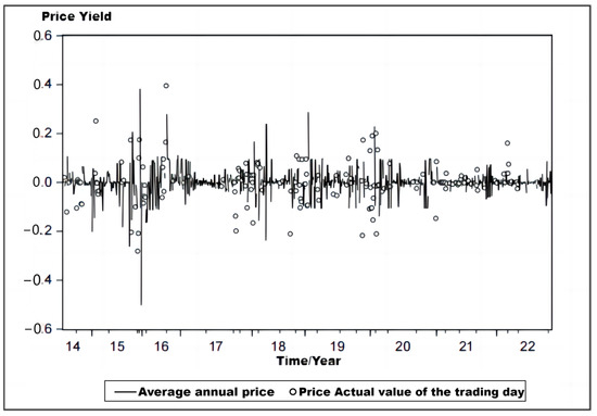
Figure 4.
Price yield fluctuation in the Shanghai carbon trading market.
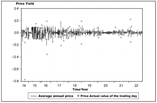
Figure 5.
Price yield fluctuation in the Guangdong carbon trading market.
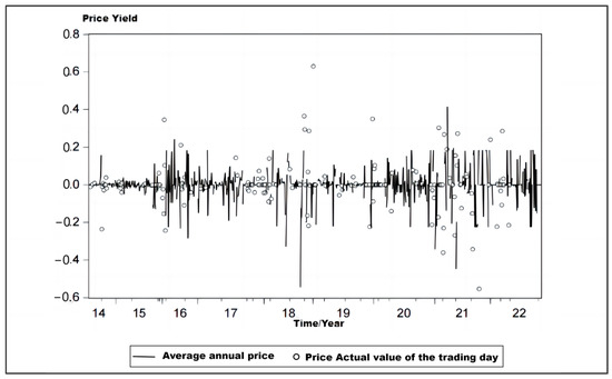
Figure 6.
Price yield fluctuation in the Beijing carbon trading market.
Overall, the average yield of the Shenzhen and Beijing ETEs was negative, and the average yield series of the remaining three ETEs were all positive, but none of them reached 0.01, indicating that the average yield of China’s ETS showed an overall low level, and China’s ETS needs further development and progress. From Table 2, it can be further found that the skewness of the Hubei and Shenzhen carbon trading markets is greater than 0, which is right-biased, in contrast, the bias of the Shanghai, Guangdong and Beijing ETSs is less than 0, which corresponds to a left bias. The skewness is less than 0 in all markets. In terms of kurtosis, the kurtosis values for all five ETS markets are greater than 3. All of these markets have the characteristics of a thick-tailed distribution and meet the basic conditions for building a GARCH family model. Figure 2, Figure 3, Figure 4, Figure 5 and Figure 6 shows the volatility of carbon trading price and yield in China’s Hubei, Shenzhen, Shanghai, Guangdong and Beijing carbon markets respectively.
4.2. Stationarity Test
In the process of modeling and analysis, in order to avoid possible statistical problems such as pseudo-regression as much as possible, it is necessary to pass a stationarity test to ensure the stability of time series data, that is, the statistical properties of the data remain unchanged at different time points. This study uses the Augmented Dickey–Fuller (ADF) unit root test to examine the persistence of the outcome series of five carbon trading experimental markets. The form of the ADF test is specified and the results are presented in Table 3. It is observed that the p-values of all regression series reject the null hypothesis at the 1% significance level. Thus, the outcome series for the five pilot carbon trading markets are robust and the ARCH series model can be used in empirical studies.
Table 3.
Carbon trading price yield stability test.
4.3. ARCH Effect Test (Autoregressive Conditional Heteroskedasticity)
4.3.1. Equilibrium Equation Construction
After confirming the stationarity of the series, autocorrelation function tests are performed on the carbon trading price returns for each pilot market. Considering the characteristics of the sample data, a lag of 20 is chosen for the autocorrelation function test. The test results show that the Q statistics of the Beijing, Shanghai, Shenzhen and Hubei sequences are significant at the 1% confidence level, rejecting the hypothesis that the squared residuals are not auto correlated. This indicates that the price return series for the four pilot markets exhibit autocorrelation. However, the autocorrelation and partial autocorrelation of Guangdong’s carbon emissions trading pilot market returns do not reject the null hypothesis at the 1% level. Thus, it is concluded that the carbon trading price return series for Guangdong does not exhibit autocorrelation. Based on the autocorrelation test results for the carbon trading price return series in each pilot market, equilibrium equations are constructed for each pilot market, as shown in Table 4.
Table 4.
Equilibrium equation for the return rate of carbon trading price.
4.3.2. ARCH Effect Test
As evident from the test results (in Table 5), the F-statistic and chi-square statistic p-values for the ARCH-LM test in all five carbon trading pilot markets are significantly smaller than the 5% critical value. This indicates that each sequence rejects the null hypothesis of “no ARCH effect in the residuals” at the 5% significance level. In other words, the price return series in China’s carbon trading markets (Beijing, Shanghai, Guangdong, Shenzhen and Hubei) exhibit ARCH effects. Therefore, clusters of ARCH models can be applied to test the volatility of the revenue series and the conditional variance of the revenue residuals can be fitted to Chinese coal trade prices using a family of GARCH models. This process allows the conditional heteroscedasticity of the auto regression to be refitted to the residual series, allowing prices to be estimated using GARCH.
Table 5.
Carbon trading price yield, ARCH effect test.
4.4. Analysis of Carbon Trading Price Return Volatility
4.4.1. Persistence of Carbon Trading Price Volatility
To ensure the accuracy of the empirical GARCH results, this study applies the GARCH (1,1), GARCH (2,1) and GARCH (1,2) models to estimate the parameters of the return series of the five experimental carbon trading markets. The most appropriate model was selected based on the AIC and SC criteria, and the GARCH (1,1) model was found to be the most appropriate. Consequently, the GARCH (1,1) model is used in the empirical analysis of the return series of the five carbon markets to solve the problem of conditional heteroscedasticity. The specific empirical results are presented in Table 6. Significantly, a higher-order GARCH model can contain any number of ARCH items and GARCH items, denoted as GARCH (p,q), where p is the order of the ARCH item and q is the order of the GARCH item, for example, GARCH (1,1) in this article means that the GARCH model contains the first-order ARCH term and the first-order GARCH term.
Table 6.
Carbon trading price, return rate and standard deviation based on GARCH (1,1) model.
The results from Table 6 indicate that the constant term coefficients in all mean equations are close to zero and statistically insignificant, suggesting that the mean return for the five carbon trading pilot markets is approximately zero. However, in the case of Guangdong’s carbon emissions trading market, the constant term coefficient in the mean equation has a p-value of 0.0046, which is significant at the 1% level, indicating that its carbon trading price return is not equal to zero.
The coefficients in the variance equations are significant at the 1% level, indicating a good fit of the GARCH (1,1) model. This implies that the null hypothesis of coefficients being equal to zero is rejected.
In all variance equations, the α coefficients are greater than 0, indicating that external shocks have some impact on carbon emission market prices. Except for Guangdong’s carbon trading market, the other pilot markets show a less sensitive response to external shocks. Among them, the impact of external shocks on Guangdong’s carbon trading market price return is the highest (1.1429), followed by Hubei, Shenzhen, Shanghai and Beijing, in descending order of sensitivity to external shocks. Compared with other pilot markets, the local government of Guangdong Province has issued a number of policies to maintain the order of the carbon emissions trading market, with relatively complete policies and a relatively mature audit system; so, due to strict government supervision, the local carbon trading market may be subject to greater external shocks.
The β coefficients in the variance equations are less than 1, indicating that external shocks have a certain persistence in impacting carbon emission market prices. Beijing’s market exhibits the strongest persistence of external shocks (0.9071). This can be explained by the fact that Beijing’s carbon market is relatively new and has low trading volumes, making it susceptible to external shocks in the long term. Additionally, Beijing’s carbon trading market has relatively high entry requirements, reducing the possibility for some companies to engage in carbon trading. The relatively lenient penalties for non-compliant companies also increase the likelihood of default to some extent. Second, the four carbon trading markets were established earlier and the market system was relatively mature. The government has, therefore, published a series of policies to maintain order in the carbon trading market. For example, the Shanghai carbon market has imposed fines on companies that do not comply with the rules, so they will have a significant long-term impact.
In the dispersion equation, the sum of α and β represents the volatility coefficient of the CO2 trading price, and the volatility of the CO2 trading price returns in each pilot market is different. Among them, the sum of the variance equation α + β for the Shanghai and Hubei carbon trading markets is significantly below 1, indicating that the resilience of carbon price volatility to external shocks is much weaker than in the other three carbon trading markets; α + β: in Shenzhen, Guangdong and Beijing is very close to 1, indicating that the period of carbon price volatility is longer in Hubei and Shanghai, while the period of volatility in Hubei and Shanghai is slightly shorter than in the other three pilot carbon trading markets.
4.4.2. Impact of Risk on Carbon Trading Price Returns
The impact of risk on carbon trading price returns is analyzed using the GARCH-M model, and the results are presented in Table 7.
Table 7.
Carbon trading price, return rate and standard deviation based on GARCH-M model.
The empirical results in Table 7 show that only the price returns of the Shanghai and Beijing ETSs are statistically significant at the 5% level, meaning that the coefficients of the standard deviation terms are significantly different from zero, while the other pilot ETSs do not exhibit a risk premium. This implies that the price returns of Shanghai and Beijing’s carbon trading markets compensate for the risks they contain, indicating the presence of risk premiums. Based on the standard deviation coefficient, the Shanghai carbon market price–return standard deviation coefficient is 0.13832, which means that the market gives a risk premium of 0.13832, while the Beijing carbon market price–return standard deviation coefficient is 0.22703, that is, for every unit of risk generated, the carbon trading pilot market will give 0.22703 units of risk compensation. In other words, as market risk increases, the carbon trading price returns also increase.
4.4.3. Asymmetry of Carbon Trading Price Volatility
Because the effects of negative and positive news on the emissions trading market can be asymmetric, this study includes a TGARCH term in the GARCH (1,1) model to test whether there is an asymmetric effect in carbon trading price volatility.
The results in Table 8 show that the coefficient γ of the TGARCH term is statistically significant at the 1% level for all pilot markets. This indicates that carbon trading price volatility exhibits an asymmetric effect, meaning that negative news and positive news have different impacts on carbon trading prices. When the macro economy improves and the Chinese government strengthens environmental pollution control, the carbon prices in Hubei, Shenzhen, Shanghai, Guangdong and Beijing will be 0.195368, 0.120010, 0.206895, 0.729500 and 0.050065 times, respectively. When there is negative news such as uncertain international climate change policy, it will have a carbon price of 0.511839, 0.256634, 0.322643, 1.556303 and 0.141624 times in Hubei, Shenzhen, Shanghai, Guangdong and Beijing, respectively. The impact of negative news (α + γ) on carbon trading prices is much greater than the impact of positive news (α) for all pilot markets. This finding aligns with the characteristics of traditional financial markets, where investors tend to be more sensitive to negative news. Even if the financial market brings equal gains and losses to investors, the happiness from gains is much smaller than the pain from equivalent losses. The higher sensitivity to bad news in Shenzhen and Shanghai may be attributed to the fact that these areas are among the regions with the highest degree of openness and economic reform in China. Companies in these regions often have extensive business dealings with other countries, making them more vulnerable to international influences and thus more sensitive to bad news. In the case of Beijing, being a region under the focus of environmental pollution control in China, it imposes stricter requirements and regulations on carbon emission trading, leading to some companies being unable to enter the market and therefore being more sensitive to bad news. The carbon markets in Hubei and Guangdong are more regulated and therefore more sensitive to negative news.
Table 8.
Carbon trading price, return rate and standard deviation based on TGARCH model.
4.5. Analysis of Carbon Trading Price Return Volatility Trends
Next, we will decompose the volatility stability of the carbon trading price returns in different scales for each domestic carbon emissions trading pilot. We will study the volatility characteristics and trends of the returns at different decomposition scales.
4.5.1. Volatility Trend Analysis Based on GARCH Model
Using the GARCH (1,1) model established earlier, we conduct a volatility trend analysis on the carbon trading price returns of each pilot market, selecting the last 339 data points of the series for prediction.
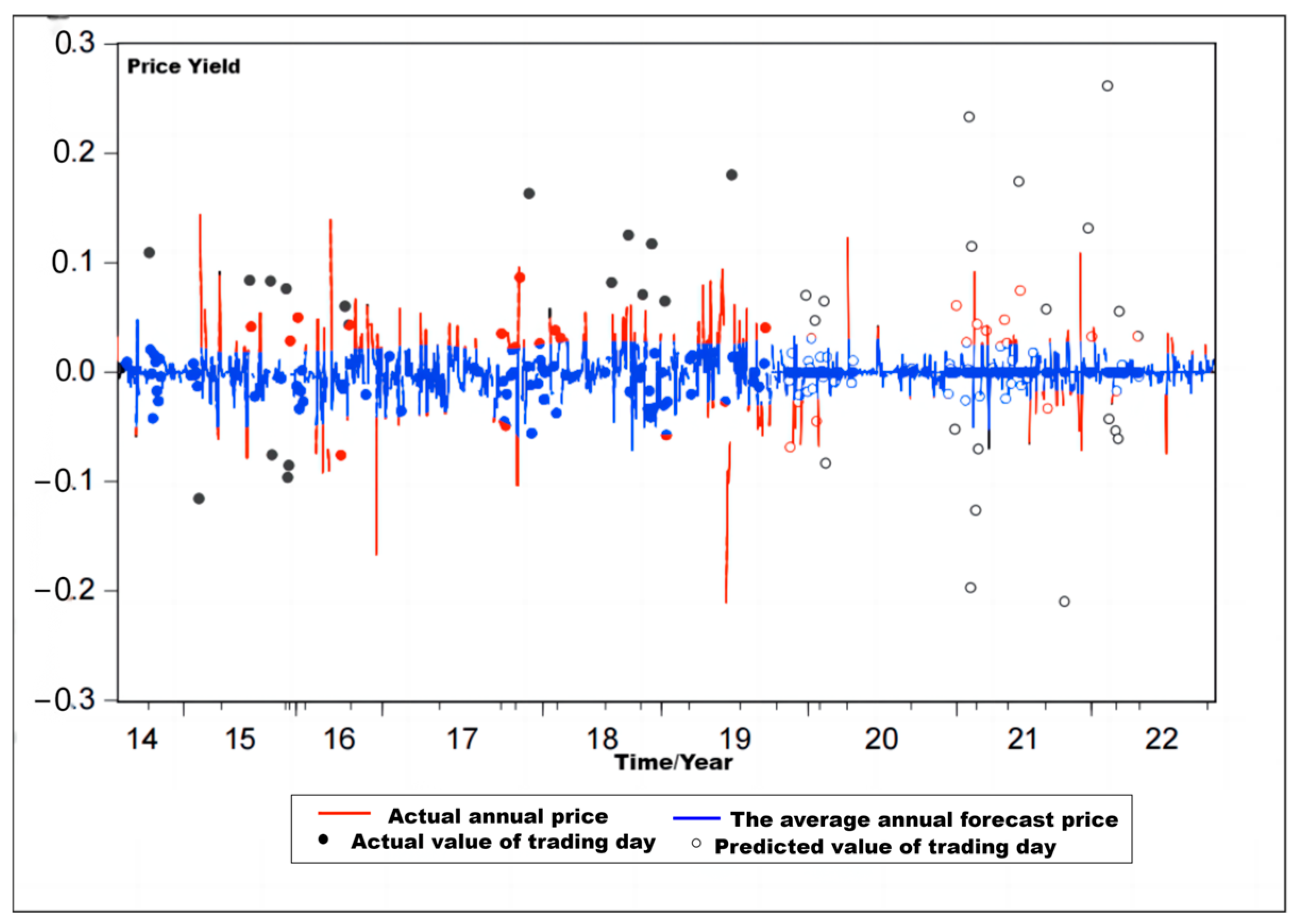
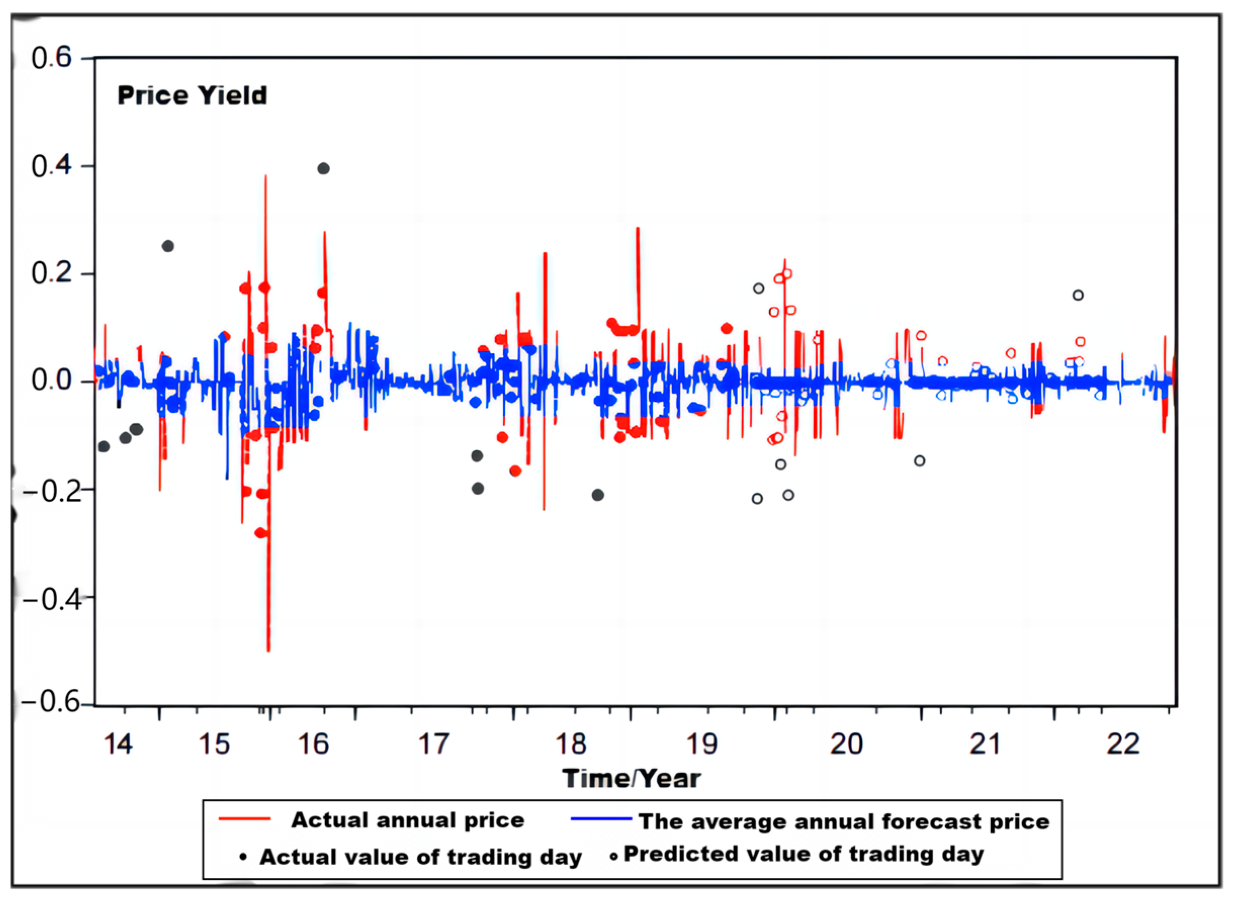
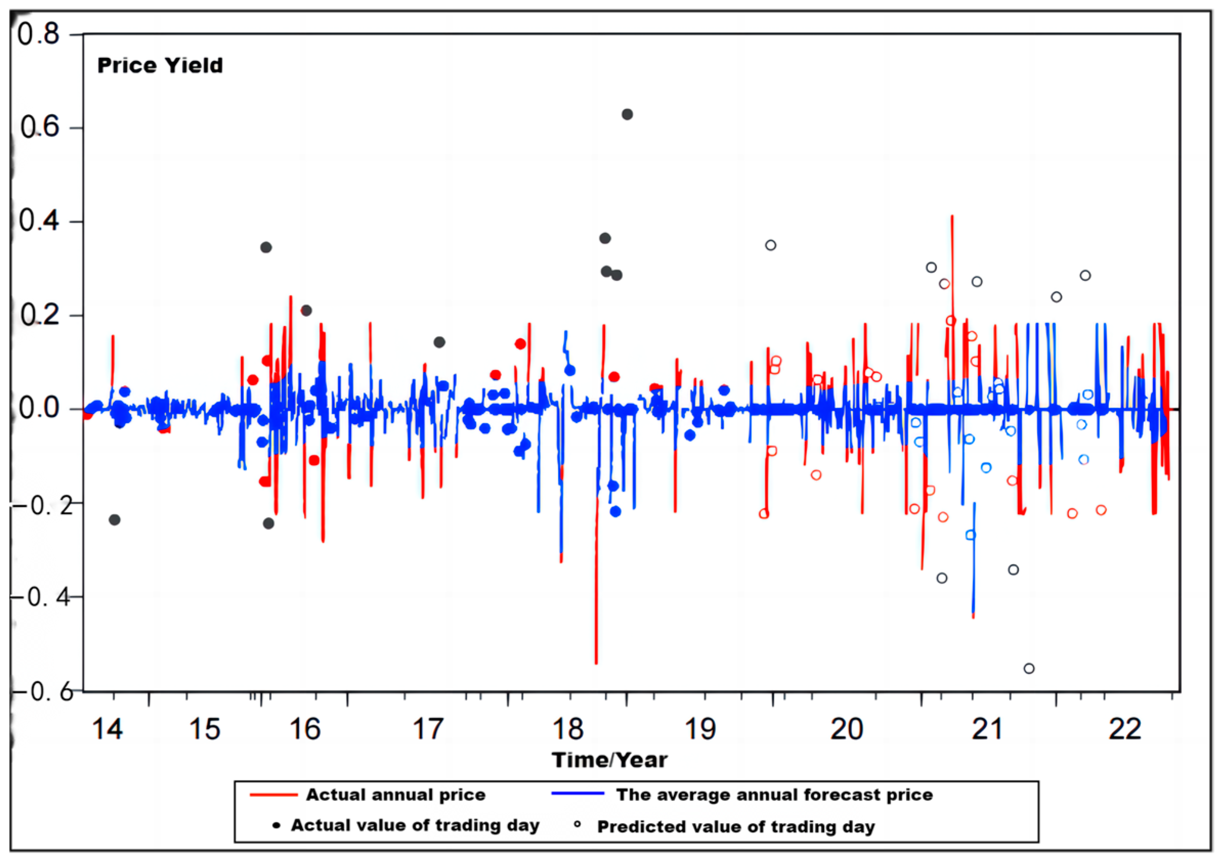
From Figure 7, Figure 8, Figure 9, Figure 10 and Figure 11, the real returns on carbon trading prices in the five carbon trading markets show a clear agglomeration area of large and small fluctuations and a large range of real value fluctuations, while the carbon trading price return rate predicted by the use of the GARCH (1,1) model for out-of-sample iterative dynamic prediction does not fluctuate much, the overall trend of the predicted value is relatively flat and the degree of deviation from the actual value is relatively large. Combined with Table 9, it can be seen that the loss function value of the model is large, which means that the model does not make good predictions of price yield, so the model does not predict well.
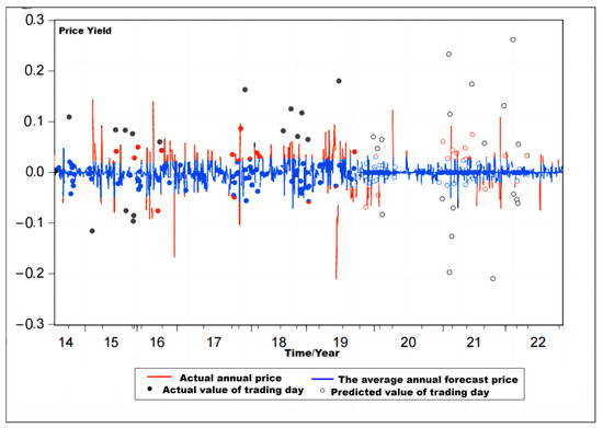
Figure 7.
Prediction of fluctuation trend of Hubei carbon trading price based on GARCH model.

Figure 8.
Prediction of fluctuation trend of Shenzhen carbon trading price based on GARCH model.

Figure 9.
Prediction of fluctuation trend of Shanghai carbon trading price based on GARCH model.
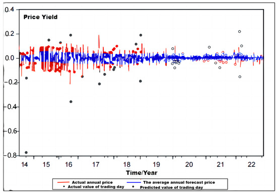
Figure 10.
Prediction of fluctuation trend of Guangdong carbon trading price based on GARCH model.
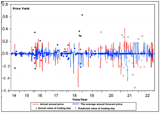
Figure 11.
Prediction of fluctuation trend of Beijing carbon trading price based on GARCH model.
Table 9.
Comparison of prediction accuracy of price–return fluctuation trends of five carbon trading pilot models with different models.
4.5.2. Carbon Trading Price Volatility Trend Based on LSTM-GARCH Hybrid Model
To facilitate the comparison with the results obtained from the GARCH model, we divided the entire selected dataset into two parts: a training set containing the first 500 data points and a test set containing the subsequent 339 data points.
The input layer of the GARCH-LSTM hybrid model consists of the estimated values of the parameters and from the GARCH model, while the output layer predicts the actual carbon trading price returns for Hubei. The LSTM model used in this study was implemented in MATLAB with the following basic parameter settings: since we are predicting the closing price, the model’s output dimension is set to 1; the input dimension includes the estimated parameters from the GARCH family model and the total number of closing prices, thus is set to 3; the number of blocks in the hidden layer is set to 10; the default learning rate is 0.00006; and the number of iterations is set to 500.
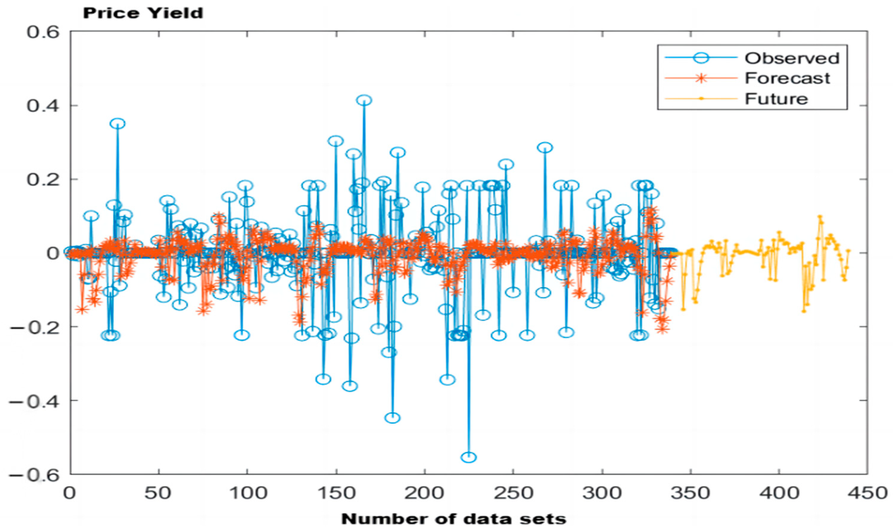
Based on the results shown in Table 9, the forecast accuracy indicators, Root Mean Square Error (RMSE) and Mean Absolute Error (MAE), for the carbon trading price returns in the five pilot markets demonstrate that the GARCH-LSTM model has better fitting performance for the carbon trading pilots in Hubei, Shenzhen and Shanghai. The smaller values of RMSE and MAE indicate that the predicted values are closer to the actual values compared to the GARCH (1,1) and LSTM models, suggesting that capturing the magnitude of carbon price fluctuations and their persistence can effectively improve the predictive performance of the model. Specifically, based on the GARCH-LSTM model, the RMSE for the carbon trading pilots in Hubei, Shenzhen and Shanghai decreases by 0.0006, 0.2993 and 0.0151, respectively, compared to the GARCH model. Furthermore, compared to the stand alone LSTM model, the RMSE decreases by 0.0007, 0.3011 and 0.0157.
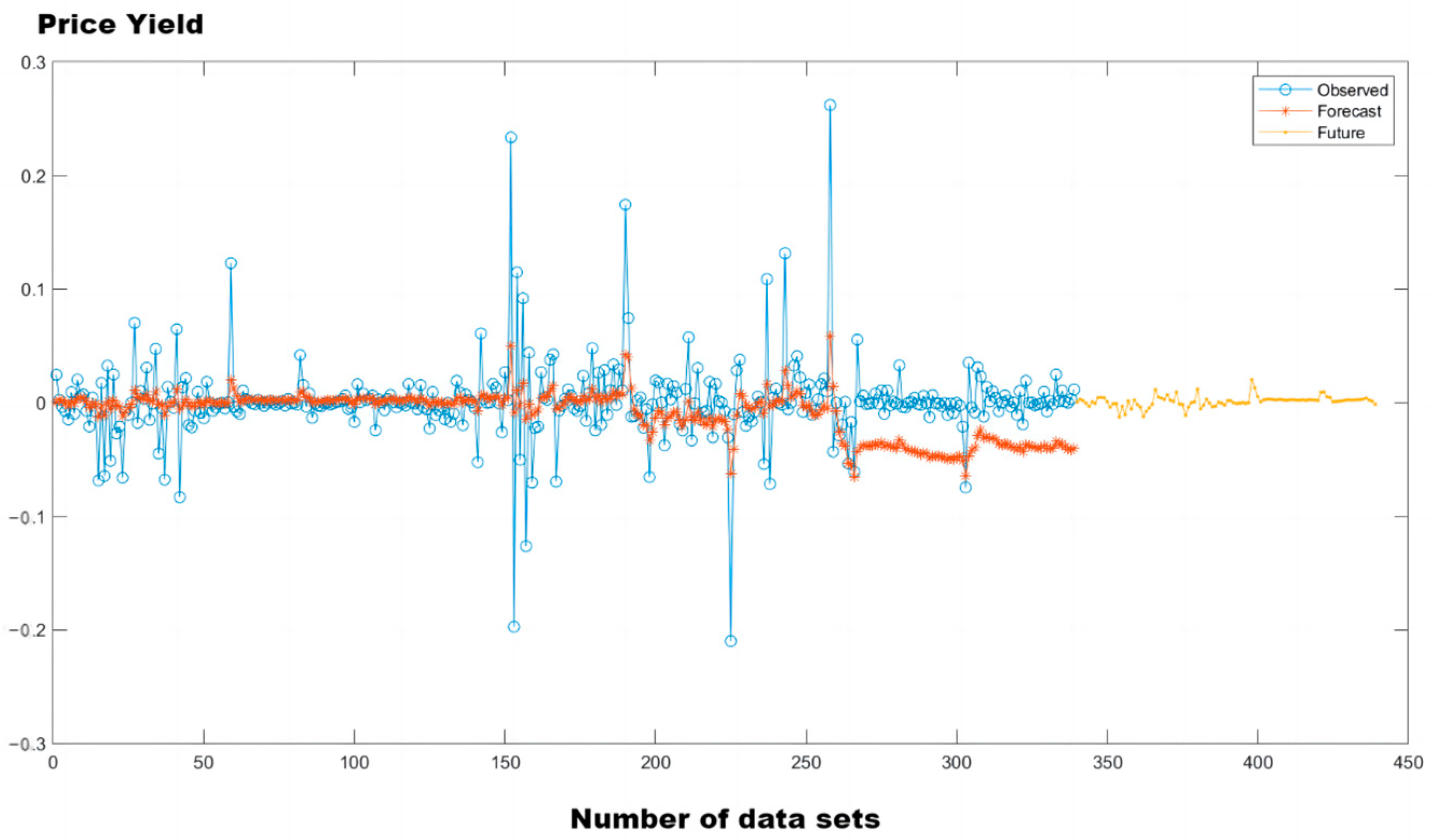
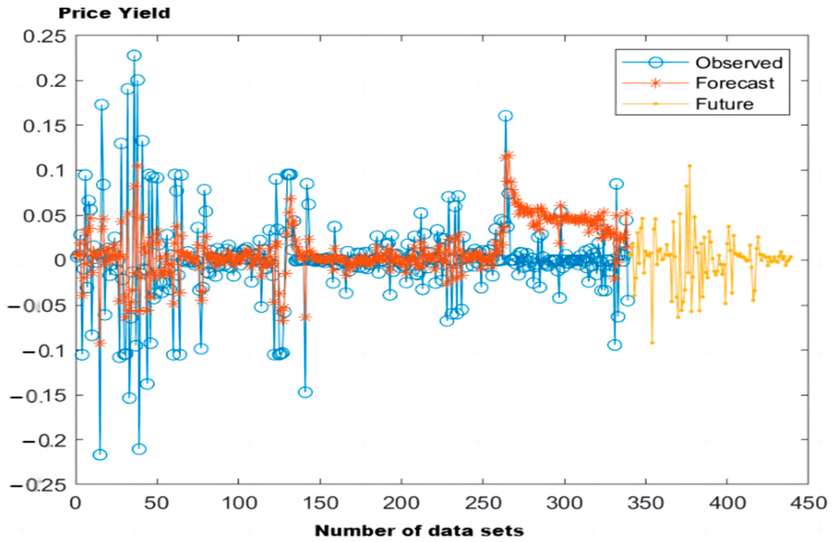
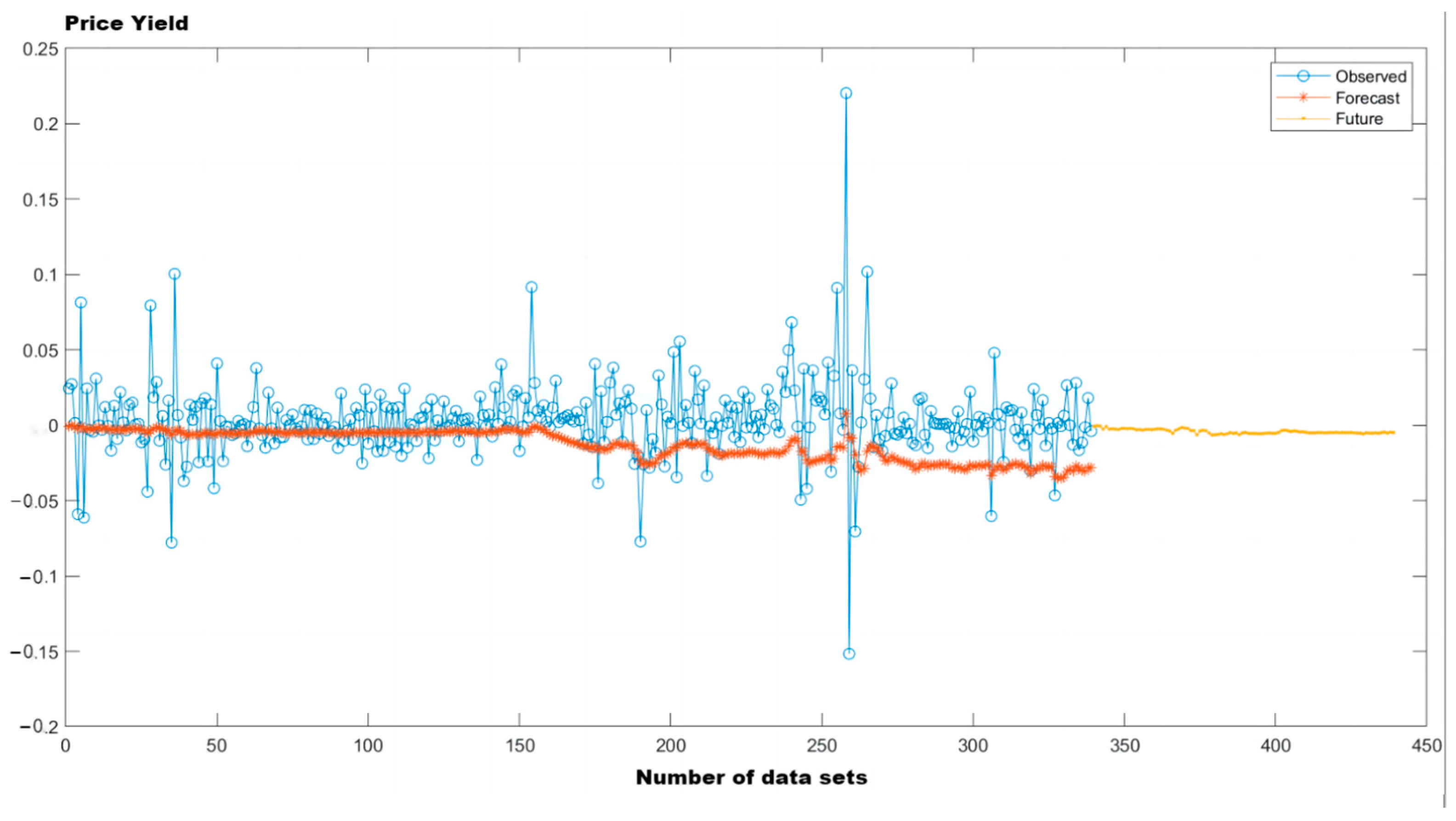
Combined with Figure 12, Figure 13, Figure 14, Figure 15 and Figure 16, the fitting fluctuation of the Hubei carbon trading market in the first 260 days is small, and the fitting fluctuation in the last 79 days is large. The 339-day fitting fluctuations of the Shenzhen carbon trading market are small, but the fluctuation range is large. The fitting fluctuation of the Shanghai carbon trading market is small in the first 260 days, and the fitting fluctuation in the last 79 days is large. The forecast value of the Guangdong carbon trading market is similar to a straight line, and the deviation from the true value is large, so the forecast effect is not good. The 339-day fitting fluctuation of the Beijing carbon trading market is small, but the fluctuation range is large. Combined with the horizontal comparison in Table 9, it is found that the price–return fluctuation prediction effect of the Hubei and Shenzhen carbon trading markets is the best, and the predicted value of the Hubei and Shenzhen carbon trading price–return fluctuation predicted by the GRACH-LSTM model has little deviation from the real value, and the fitting fluctuation is small throughout the period, which further indicates that the GRACH-LSTM hybrid model is better than the single model.
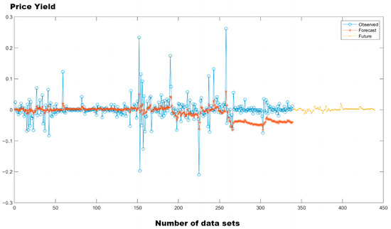
Figure 12.
Prediction of fluctuation trend of Hubei carbon trading price based on GRACH-LSTM model.
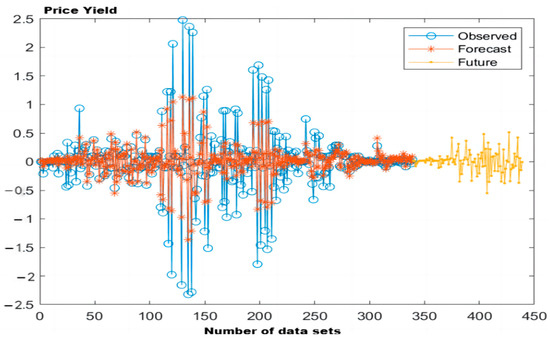
Figure 13.
Prediction of fluctuation trend of Shenzhen carbon trading price based on GRACH-LSTM model.

Figure 14.
Prediction of fluctuation trend of Shanghai carbon trading price based on GRACH-LSTM model.

Figure 15.
Prediction of fluctuation trend of Guangdong carbon trading price return based on GRACH-LSTM model.

Figure 16.
Prediction of fluctuation trend of Beijing carbon trading price based on GRACH-LSTM model.
The main reasons for the error between the prediction line and the actual line of the Hubei carbon trading market are that (1) due to the influence of China’s economic macro factors, the carbon trading price shows some abnormal fluctuations, and the actual value has individual outliers, for example, the prediction error of the Hubei forecast results is small in the first 260 sample data and relatively large after that, that is, after 28 February 2022, macro factors are external factors affecting the fluctuation of carbon trading prices. Including economic, political and social factors, as well as natural environmental conditions, etc., macro factors are complex and difficult to quantify, and relevant information is not included in the prediction model. (2) Compared with other prediction charts, Figure 12 has a smaller scale interval (0.1), which makes the difference between the predicted value curve and the actual value curve more significant. At the same time, existing studies have failed to solve this problem. In order to better solve this problem, a prediction model of high-dimensional macro information is considered to see whether the prediction accuracy can be further improved.
At the same time, based on the predictions, the carbon emission prices for the next 100 days are forecasted and the five carbon trading prices and return fluctuation trends are shown in yellow (see Figure 12, Figure 13, Figure 14, Figure 15 and Figure 16). The figure shows that the Hubei carbon market’s carbon price return fluctuation over the next 100 days is small, the Shenzhen carbon market’s carbon price return fluctuation over the next 100 days is small but large, the Shanghai carbon trading market’s carbon trading price return adjustment and fluctuation after 100 days is large, and the Guangdong carbon trading market’s carbon trading price returns are almost linear and do not fully reflect the fluctuations in carbon trading prices. The model cannot be used successfully for forecasting as it cannot fully reflect the price situation of the Guangdong carbon market. Finally, prices and returns in the Beijing carbon market over the next 100 days will fluctuate significantly. With the exception of the Guangdong carbon market, the carbon price returns of the other four carbon markets show that the GRACH-LSTM model is good at predicting future price returns.
5. Conclusions and Implications
5.1. Conclusions
This study uses the ARCH model to analyze the volatility of carbon trading prices in China’s carbon trading market and performs a predictive analysis of carbon trading price returns. The main results are as follows:
(1) The correct testing method and model selection are helpful to accurately and effectively understand the carbon pricing mechanism and its price fluctuation characteristics. In this work, two test methods, namely the ADF unit root test and ARCH effect test, are used to test the stationarity and autocorrelation of price return series, and the GARCH family model is used to study the volatility aggregation, risk premium and asymmetry of carbon trading price return. The research results show that all of the pilot markets in China have certain volatility and clustering characteristics, and only the carbon markets in Shanghai and Beijing show risk premium characteristics. On the whole, the development of China’s carbon trading market is relatively immature. In addition, the carbon price fluctuation in the carbon market has an asymmetric effect, and negative and positive news have a great difference on the carbon price. By constructing the GARCH family model for analysis, the identification results of the price fluctuation characteristics of the carbon trading market are more accurate.
(2) Deep machine learning methods help improve predictions. Comparing and analyzing the prediction performance of multiple combined models, the experimental results show that the GARCH-LSTM model performs better in predicting carbon trading prices. Since the impact size and persistence of carbon price fluctuations are captured, the deviation between the predicted value and the real value is obviously narrowed, which is manifested as less fitting fluctuation in the whole period. Based on the GARCH-LSTM model, the Root Mean Square Errors (RMSE) for the carbon trading pilots in Hubei, Shenzhen and Shanghai are significantly reduced compared to the GARCH model, showing improvements of 0.0006, 0.2993 and 0.0151, respectively. Moreover, compared to the standalone LSTM model, the RMSE improvements for the three pilot markets are 0.0007, 0.3011 and 0.0157, respectively, indicating the effectiveness of the model’s predictive results.
(3) As a traditional econometric method, the GARCH model has some defects in the analysis and prediction of carbon price fluctuation. Deep machine learning methods have the characteristics of using fewer assumptions and modeling constraints and can better solve complex models and make accurate predictions. This paper innovatively proposes to combine the information obtained from the traditional econometric model with the neural network model, which is to say, add the LSTM neural network model on the basis of the GARCH model to build a hybrid GARCH-LSTM model containing multiple GARCH-type models, in which multiple GARCH-type model parameters are combined. For example, the magnitude α_i representing the wave shock in GARCH(1,1), the wave β_j representing the past persistence, and the direction α representing the wave shock in GARCH-M(1,1) are all used as inputs to the LSTM model, and other explanatory variables are introduced. By learning the characteristics of input variables, the neural network can help to predict the carbon trading price, thereby improving the prediction performance of the hybrid model and providing a new way to study the volatility and prediction of financial time series.
5.2. Implications
Compared with the mature and advanced EU-ETS, EU-ETS shows a good feature of small fluctuation amplitude and short duration from both the medium and short term perspective, while the carbon price fluctuation in China’s carbon trading market is concentrated and the fluctuation duration is longer.
This can be attributed to the imperfect mechanism of the carbon market, the low liquidity of the market and the small number of transaction types. This conclusion leads to a number of recommendations for policymakers.
Policymakers should urgently improve carbon market disclosure systems and monitoring mechanisms to reduce information uncertainty, prevent market price volatility, avoid market risks, improve the liquidity of market transactions, innovate financial carbon derivatives and facilitate the entry of third-party intermediaries such as financial institutions into carbon markets. Derivative financial instruments such as carbon futures and options can be applied to carbon trading markets. The upper and lower limits of the carbon price can be set to control the volatility of the carbon price and prevent the carbon price from being too high or too low, causing the carbon trading market to stop functioning. Appropriate policies can be developed to determine the level of the carbon price in response to dynamic changes in the carbon trading market. The circulation of money influencing the carbon price and stabilizing the carbon price through, for example, open market operations, is a key policy direction for the carbon trading market.
From the short-term perspective of market participants, the Chinese carbon market is less active, with participants more risk-averse and a lack of diversity in market instruments. More specifically, the Hubei carbon market is subject to short-term price fluctuations due to external shocks, making it suitable for risk-averse participants and offering better opportunities for investment returns. The Shanghai and Beijing carbon markets have a risk premium and are best suited to participants who are willing to take risks and earn excess returns. In the medium to long term, it is difficult for participants to interpret market information from the uncertainty of carbon prices, and including more accurate carbon price forecasts in the investment decision-making process can help participants and reduce investment risks.
Author Contributions
S.L. performed the data analyses and wrote the manuscript; Y.Z. contributed significantly to the analysis and manuscript preparation; J.W. contributed to the conception of the study; D.F. helped perform the analysis with constructive discussions. All authors have read and agreed to the published version of the manuscript.
Funding
This work was supported by the Shaanxi Provincial Philosophy and Social Science Planning Project (Project NO. 2021D049), Shaanxi Provincial Education Department Scientific Research Project (Project NO. 21JK0281), Xi’an Social Science Planning Fund Project (Project NO. 22FZ97), Shaanxi Provincial National College Students Innovation and Entrepreneurship Training Project (Project NO. 202110705012) and The Key Research Base of Humanities and Social Sciences of Ministry of Education major project of the 13th Five-Year Plan (Project NO. 17JJD790016).
Institutional Review Board Statement
Not applicable.
Informed Consent Statement
Written informed consent was obtained from the patient for publication of the case report and any accompanying images. A copy of the written consent is available for review by the Editor-in-Chief of this journal.
Data Availability Statement
The datasets used or analyzed during the current study are available from the corresponding author on reasonable request.
Conflicts of Interest
The authors declare no conflicts of interest.
References
- Jia, Z.; Lin, B. CEEEA2.0 model: A dynamic CGE model for energy environment-economy analysis with available data and code. Energy Econ. 2022, 112, 106117. [Google Scholar] [CrossRef]
- Böhringer, C.; Hoffmann, T.; Manrique-de-Lara-Peñate, C. The efficiency costs of separating carbon markets under the EU emissions trading scheme: A quantitative assessment for Germany. Energy Econ. 2006, 28, 44–61. [Google Scholar] [CrossRef]
- Mansanet-Bataller, M.; Pardo, A.; Valor, E. CO2 prices, energy and weather. Energy 2007, 28, 73–92. [Google Scholar]
- Chevallier, J. A model of carbon price interactions with macroeconomic and energy dynamics. Energy Econ. 2011, 33, 1295–1312. [Google Scholar] [CrossRef]
- Cong, R.; Lo, A.Y. Emission trading and carbon market performance in Shenzhen, China. Appl. Energy 2017, 193, 414–425. [Google Scholar] [CrossRef]
- Zhang, Y.J.; Wei, Y.M. Mean reversion of international carbon futures prices: An empirical analysis based on EU ETS. Syst. Eng. Theory Pract. 2011, 31, 214–220. [Google Scholar]
- Lv, Y.B.; Shao, L.B. Study on the fluctuation characteristics of carbon emission price in China—Based on the analysis of GARCH family model. Price Theory Pract. 2015, 12, 62–64. [Google Scholar]
- Zhang, J.; Sun, L.H.; Xing, Z.C. Research on price volatility of China’s carbon emission trading market: Based on data analysis of pilot carbon emission market trading prices in six cities including Shenzhen, Beijing and Shanghai. Price Theory Pract. 2018, 1, 57–60. [Google Scholar]
- Lv, J.Y.; Wang, T.F. Long-term memory and leverage effect of price fluctuations in China’s carbon emission allowance market: A case study of Hubei Carbon Emission Rights Trading Center. Price Mon. 2019, 10, 29–36. [Google Scholar]
- Zhang, J.; Cui, Y.L. Comparative study on price trend characteristics of China’s carbon trading market: Based on sample data analysis of carbon trading market in Hubei, Guangdong and Shenzhen. Price Theory Pract. 2021, 5, 161–164+196. [Google Scholar]
- Kainuma, M.; Matsuoka, Y.; Morita, T. Analysis of post-Kyoto scenarios: The Asian-Pacific Integrated Model. Energy J. 1999, 20, 207–220. [Google Scholar] [CrossRef]
- Li, W.; Lu, C. The research on setting a unified interval of carbon price benchmark in the national carbon trading market of China. Appl. Energy 2015, 155, 728–739. [Google Scholar] [CrossRef]
- Zhang, C.; Yang, X.Z. Price prediction of China’s regional carbon market based on multi-frequency combination model. Syst. Eng. Theory Pract. 2016, 36, 3017–3025. [Google Scholar]
- Zhao, L.D.; Wang, H.X. Research on carbon trading price prediction: A case study of Shenzhen. Price Theory and Practice. 2019, 2, 76–79. [Google Scholar]
- Wei, Y.; Zhang, J.H.; Chen, X.D. China’s carbon emission trading price prediction method based on DMS and DMA: Empirical evidence from Hubei carbon market. Syst. Eng. 2022, 40, 1–16. [Google Scholar]
- Liu, Z.B.; Huang, S. Carbon option price forecasting based on modified fractional Brownian motion optimized by GARCH model in carbon emission trading. N. Am. J. Econ. Financ. 2021, 55, 101307. [Google Scholar] [CrossRef]
- Gong, W.F.; Wang, L.P.; Wang, C.H.; Gao, Z.F. Research on the Fluctuation Characteristics of Carbon Emission Trading Price in China’s Carbon Emission Allowance Market—An Empirical Analysis of Five Carbon Trading Pilots. China Soft Sci. 2022, 4, 149–160. [Google Scholar]
- Yun, P.; Zhang, C.; Wu, Y.; Yang, X.; Wagan, Z.A. A Novel Extended Higher-Order Moment Multi-Factor Framework for Forecasting the Carbon Price: Testing on the Multilayer Long Short-Term Memory Network. Sustainability 2020, 12, 1869. [Google Scholar] [CrossRef]
- Zhao, Y.H.; Zhao, H.R.; Li, B.H.; Wu, B.X.; Guo, S. Point and interval forecasting for carbon trading price: A case of 8 carbon trading markets in China. Environ. Sci. Pollut. Res. 2023, 30, 49075–49096. [Google Scholar] [CrossRef] [PubMed]
- Hochreiter, S.; Schmidhuber, J. Long Short-term Memory. Neural Comput. 1997, 9, 1735–1780. [Google Scholar] [CrossRef] [PubMed]
- Dey, P.; Chaulya, S.K.; Kumar, S. Hybrid CNN-LSTM and IoT-based coal mine hazards monitoring and prediction system. Process Saf. Environ. Prot. 2021, 152, 249–263. [Google Scholar] [CrossRef]
- Marzouk, M.; Elshaboury, N.; Abdel-Latif, A.; Azab, S. Deep learning model for forecasting COVID-19 outbreak in Egypt. Process Saf. Environ. 2021, 153, 363–375. [Google Scholar] [CrossRef]
- Chen, W.; Xu, H.L.; Jia, L.F.; Gao, Y. Machine learning model for Bitcoin exchange rate prediction using economic and technology determinants. Int. J. Forecast. 2021, 37, 28–43. [Google Scholar] [CrossRef]
- Yang, D.; Wang, J.; Yan, X.; Liu, H. Subway air quality modeling using improved deep learning framework. Process Saf. Environ. Prot. 2022, 163, 487–497. [Google Scholar] [CrossRef]
- Jianwei, E.; Ye, J.; He, L.; Jin, H. Energy price prediction based on independent component analysis and gated recurrent unit neural network. Energy 2019, 189, 116278. [Google Scholar]
- Wang, X.L.; Zhang, Y.; Liu, P.Z.; Wen, F.J.; Ren, W.M.; Zheng, Y.; Wang, G.; Yan, B. Analysis of apple price prediction based on LSTM and GARCH family combination model. J. Shandong Agric. Univ. (Nat. Sci. Ed.) 2021, 52, 1055–1062. [Google Scholar]
- Hao, Y.; Tian, C. A hybrid framework for carbon trading price forecasting: The role of multiple influence factor. J. Clean. Prod. 2020, 262, 120378. [Google Scholar] [CrossRef]
- Adekoya, O.B. Predicting carbon allowance prices with energy prices: A new approach. J. Clean. Prod. 2021, 282, 124519. [Google Scholar] [CrossRef]
- Sun, W.; Zhang, C. Analysis and forecasting of the carbon price using multi—Resolution singular value decomposition and extreme learning machine optimized by adaptive whale optimization algorithm. Appl. Energy 2018, 231, 1354–1371. [Google Scholar] [CrossRef]
- Xu, H.; Wang, M.; Jiang, S.; Yang, W. Carbon price forecasting with complex network and extreme learning machine. Phys. A Stat. Mech. Appl. 2020, 545, 122830. [Google Scholar] [CrossRef]
- Huang, Y.C.; He, Z. Carbon price forecasting with optimization prediction method based on unstructured combination. Sci. Total Environ. 2020, 725, 138350. [Google Scholar] [CrossRef]
- Zhu, J.; Wu, P.; Chen, H.; Liu, J.; Zhou, L. Carbon price forecasting with vibrational mode decomposition and optimal combined model. Phys. A Stat Mech. Appl. 2019, 519, 140–158. [Google Scholar] [CrossRef]
- Jianwei, E.; Ye, J.; He, L.; Jin, H. A denoising carbon price forecasting method based on the integration of kernel independent component analysis and least squares support vector regression. Neurocomputing 2021, 434, 67–69. [Google Scholar]
- Yang, S.M.; Chen, D.J.; Li, S.L.; Wang, W.J. Carbon price forecasting based on modified ensemble empirical mode decomposition and long short-term memory optimized by improved whale optimization algorithm. Sci. Total Environ. 2020, 716, 137117. [Google Scholar] [CrossRef] [PubMed]
- Huang, Y.; Dai, X.; Wang, Q.; Zhou, D. A hybrid model for carbon price forecasting using GARCH and long short-term memory network. Appl. Energy 2021, 285, 116485. [Google Scholar] [CrossRef]
- Kakade, K.; Jain, I.; Mishra, A.K. Value-at-Risk forecasting: A hybrid ensemble learning GARCH-LSTM based approach. Resour. Policy 2023, 78, 102903. [Google Scholar] [CrossRef]
- Bollerslev, T. Generalized autoregressive conditional heteroscedasticity. J. Econom. 1986, 31, 307–327. [Google Scholar] [CrossRef]
- Engle, R.F.; Lilien, D.M.; Robins, R.P. Estimating time varying risk premia in the structure: The ARCH-M model. Econometrica 1987, 55, 391–407. [Google Scholar] [CrossRef]
- Glosten, L.R.; Jagannathan, R.; Runkle, D.E. On the relation between the expected value and the volatility of the nominal excess return on stocks. J. Financ. 1993, 48, 1779–1801. [Google Scholar] [CrossRef]


Disclaimer/Publisher’s Note: The statements, opinions and data contained in all publications are solely those of the individual author(s) and contributor(s) and not of MDPI and/or the editor(s). MDPI and/or the editor(s) disclaim responsibility for any injury to people or property resulting from any ideas, methods, instructions or products referred to in the content. |
© 2024 by the authors. Licensee MDPI, Basel, Switzerland. This article is an open access article distributed under the terms and conditions of the Creative Commons Attribution (CC BY) license (https://creativecommons.org/licenses/by/4.0/).