Article

Spatiotemporal Patterns and Drivers of Trade-Offs and Synergy in the Beijing–Tianjin Sand Source Control Project: A Bayesian Belief Network-Based Analysis

Institute of Ecological Protection and Restoration, Chinese Academy of Forestry, Beijing 100091, China
*
Author to whom correspondence should be addressed.
Sustainability 2024, 16(4), 1617; https://doi.org/10.3390/su16041617
Submission received: 19 December 2023 / Revised: 1 February 2024 / Accepted: 13 February 2024 / Published: 15 February 2024

Abstract

:
Understanding the interactions between ecosystem services is the foundation for optimizing ecosystem management and improving human well-being. However, studies on the driving mechanism of ecosystem service relationship formation in arid and semiarid climates are scarce. The Beijing–Tianjin Sand Source Control Project (BTSSCP) has been underway for more than 20 years (2001–2022), and a comprehensive scientific assessment of the effects of its implementation is important for managing ecosystems more efficiently. Taking the BTSSCP region as a study area, four ecosystem services (water conservation (WC), soil conservation (SC), wind erosion control (WEC), and net primary productivity (NPP)) were quantified and mapped in 2000, 2010, and 2020. In this study, a Bayesian belief network (BBN) model was used to analyze ecological processes and determine the relationship between the potential influencing factors and ecosystem services. A sensitivity analysis identified the key factors affecting ecosystem service supply on the basis of a Bayesian belief network simulation. The results showed an increasing trend for four ecosystem services over the past 20 years. Regarding spatial distribution, WC, SC, and NPP exhibited an overall “high in the east and low in the west” pattern, while the spatial distribution of WEC was more dispersed. The intensity of the trade-offs among WC, SC, and NPP has increased, while that of the trade-offs between the rest of the variables has decreased in the BTSSCP over the past 20 years. The results of the Bayesian network modeling indicated that precipitation, NDVI, land use, and temperature were the major variables influencing the strength of ecosystem service trade-offs. The conditional probabilities of the key variables in different states showed that the Sunit Left Banner, Sunit Right Banner, and other areas of control of the desertification of arid grassland had a high probability of trade-offs in WC_SC and SC_NPP. However, the probability of a trade-off between WEC and NPP was higher in the southeastern part of the Yanshan Hills Mountain Water Source Reserve than in the other regions; thus, it should be prioritized as an area for ecological restoration in future planning. This paper provides a scientific reference for the effective protection of ecosystems and the formulation of sustainable policies.

1. Introduction

Ecosystem services refer to the benefits that humans directly or indirectly receive from natural ecosystems, and are essential for human survival, livelihood, and well-being [1,2]. As a bridge connecting the social and ecological systems, ESs have a significant impact on ensuring regional sustainability [3,4]. Multiple ecosystem services exhibit synergistic or trade-off-based relationships with one another owing to spatial heterogeneity [5,6,7]. Understanding how to efficiently and fairly manage ecosystem service trade-offs is a key scientific problem in ecosystem management research [8,9]. Optimizing the spatial heterogeneity of ecosystem service trade-offs may play an important role in improving the effects of regional ecosystem services and ensuring sustainable development.
Researchers have applied a variety of approaches to analyze the trade-offs and synergy in ecosystem services, including spatial mapping [10], the analysis of the mechanisms driving such trade-offs [11], statistical recognition [12], and scenario simulation [13]. Although a correlation analysis can be used to identify the relationships between ecosystem services, it cannot reflect their spatial distribution [14]. An ecosystem service trade-off varies spatiotemporally due to uncertainty in the factors driving it [15]. Research on the drivers of ecosystem service trade-offs has largely focused on the analyses of linear relationships using the least-squares model (OLS), geographically weighted regression (GDM), and geographical detector models (GWR) [16,17,18]. Nonlinear relationships that may influence ecosystem service trade-offs have mostly been ignored; as such, the manner in which indirect factors influence the spatiotemporal patterns of ecosystem service trade-offs and the underlying drivers remains largely unknown. Thus, the intrinsic mechanisms of the trade-offs and synergies among ESs and the forces driving them still need to be examined [19]. Network models are becoming increasingly popular as a means of analyzing ecosystem service trade-offs. In the case of sustainable forest management, for instance, trade-offs among the wood provisioning ecosystem services and other forest ecosystem services at the landscape level were analyzed using a BBN model to guide decision-making toward sustainable forestry [20]. Furthermore, the BBN model has also been used to determine the factors driving trade-offs among NPP, WY, and SC in the karst regions of China, which is beneficial for ecosystem service optimization for ecological restoration and decision making [21]. To represent the nonlinear relationships between the driving factors of the ecosystem service value, Liu et al. used a BBN model to simulate the values of ecosystem services under different scenarios in Xinjiang Province [22].
Owing to the graphical nature and probabilistic basis of a BBN, nonlinear relationships can be expressed, involving natural factors, expert knowledge, and anthropogenic factors [23]. A BBN can combine quantitative and qualitative data in an intricate network of relationships through simple and understandable graphical structures, and this can help optimize ecosystem management [24]. In addition, a BBN can incorporate uncertainties from input nodes in the model, especially when the data are incomplete or missing, because they are based on probability [25]. Few studies, however, have used Bayesian networks to fully explore the underlying mechanisms of ecosystem service trade-offs by coupling natural, socio-economic, and ecological factors to optimize spatial patterns in ecological restoration projects areas.
The BTSSCP is an important national ecological restoration project in China (CANM-EP), especially in the context of strong sandstorms and dust storms in North China [26]. The first stage (2001–2010) covered 75 counties in Beijing, Tianjin, Hebei, Shanxi, and Inner Mongolia, and involved an investment of USD 8.11 billion in a series of ecological practices to curb sandy expansions and reduce the frequency of sandstorms in the relevant regions [27]. Recent studies have shown that the implementation of the BTSSCP has significantly improved the status of local vegetation, reduced soil erosion, and enhanced the carbon stock [28,29]. Such significant ecosystem services benefits may be accompanied by important trade-offs [30]. Although the improved vegetation coverage in the grasslands of the Hunshandake Sandy Subzone and Horqin Sandy Subzone (a typical region in the BTSSCP) enhanced their water conservation capacities [31], afforestation consumes more water than the restoration of grassland and undeveloped land in arid and semiarid China [32,33]. Exploring the relationship between regional vegetation restoration on BTSSCP ecosystem services and ecosystem service trade-offs is important for improving ecological restoration strategies and realizing sustainable development in arid and semiarid climates. Nevertheless, few studies have analyzed the influencing factors of ecosystem service trade-offs in the BTSSCP. This lack of research will in turn affect the formulation and implementation of policies for ecological protection in the future.
Regarding the BTSSCP as a major source of sand and dust for the dust storms and sandstorms of Northern China, WEC, WC and SC are important ecosystem services in the area [34,35]. NPP can directly reflect the productive capacity change in vegetation [27]. Given the gaps in information identified above, we assessed the WC, SC, WEC, and NPP (Table S1), and the trade-offs between ecosystem services in the BTSSCP from 2000 to 2020. Our hypothesis was that ecological engineering will alter the trade-off relationships between NPP, WC, SC, and WEC in the BTSSCP and that vegetation restoration will boost an NPP–WC trade-off. We used the correlation coefficient and the RMSE index to describe the spatial patterns of the strength of trade-offs among these four ecosystem services. We developed a BBN model and applied sensitivity analysis to identify the key factors driving the pattern of ecosystem service trade-offs in the BTSSCP. The aims were (1) to explore the spatiotemporal patterns of changes in the four main ecosystem services of the BTSSCP; (2) to analyze the forces driving ecosystem service trade-off; and (3) to identify areas for the optimization of the spatial patterns of trade-offs in ecological services and potentially provide scientific foundations for future engineering projects.

2. Materials and Methods

2.1. Study Area Overview

The entire region included during the first stage of the BTSSCP was used as the study area (Figure 1). The Beijing–Tianjin Sandstorm Source Control Project (109°30′–114°20′ E, 38°50′–46°40′ N) extends from the Darhan Muming’an United Banner of Inner Mongolia in the west to the Ar Horqin Banner of Inner Mongolia in the east, and from Dai County of Shanxi Province in the south to the East Ujimqin Banner of Inner Mongolia in the north. It covers an area of 458,000 km2 across 75 counties in Beijing, Tianjin, Hebei, Shanxi, and Inner Mongolia, of which 22.23% is sandy land. Soil types in the study area are varied and include chestnut soils, brown soils, black soils, and stony soils, of which chestnut soils are the most widely distributed. The vegetation type is dominated by temperate deciduous broad-leaved forests and warm temperate deciduous broad-leaved forests. From south to north, the climate zone changes from warm temperate and semi-humid to temperate semi-arid, temperate arid, and finally temperate and extraordinarily arid, with an average annual atmospheric temperature ranging from 0.6 to 12 °C, and 95–595 mm of precipitation. The topography of the northwest is higher than that of the southeast, with diverse landforms. We divided the study area into four zones: the sandy area of arid grassland, Hunshandake sandy land, Psturage ecotone sandy land, and Yanshan mountain water conservation area.

2.2. Data Sources

We processed remote sensing spatial data on the land use, meteorology, conditions of the soil, NPP, and NDVI on the ArcGIS 10.6 platform (RedLands, CA, USA) for analysis (Table 1). The data were officially verified and calibrated to ensure that they could be used for analysis.

2.3. Methods of Assessment

2.3.1. Water Conservation

Water conservation refers to the amount of water that infiltrates the ground after precipitation subtracts evapotranspiration and surface runoff [36,37]. Water yields were calculated using the InVEST (Integrated Valuation of Ecosystem Services and Tradeoffs) model (Palo Alto, CA, USA). The actual water yield was obtained using the water balance method [38]. We used this information to evaluate water conservation in the BTSSCP.
A E T X J P X = 1 + ω X R X J 1 + ω X R X J + 1 R X J
R X J = E T 0 × K X J P X
ω x = Z A W C X P X + 1.25
Y X J = 1 A E T X J P X × P X
W C = m i n 1 , 249 V e l o c i t y × m i n 1 , 0.9 × T I V e l o c i t y × m i n 1 , K s a t 300 × Y X J
Here, WC is the capacity for water conservation (mm), Velocity is the coefficient of flow, TI is the topographical index, and K s a t is the saturated hydraulic conductivity of soil. ωX is the ratio of annual potential evapotranspiration to precipitation. AWCX is the available water yield of the plant. AETXJ is the average evapotranspiration calculated using the InVEST model, YXJ is its calculated water yield, PX is the annual precipitation for raster X, and RXJ is the Bydyko dryness index for land use type J. ET0 is the reference crop evapotranspiration, and KXJ refers to the plant evapotranspiration coefficient for the land use types of raster X. Z is a seasonal factor that varies across regions.

2.3.2. Soil Conservation

Vegetation can control soil erosion by preventing or limiting the detachment and transport of soil particles in water or air [39]. We used the RUSLE (Revised Universal Soil Loss Equation) model and ArcGIS 10.6 software to estimate soil erosion [40]:
R K L S = R × K × L S
U S L E = R × K × L S × P × C
S C = R K L S U S L E
where SC represents soil conservation, t·(hm2·a)−1; RKLS is potential soil erosion; and USLE is the actual amount of soil erosion. R is the erosivity of rainfall, MJ·mm/(hm2·ha·a)−1; K is the erodibility of soil, t·h·(hm2·MJ); L is the length of the slope; S is its gradient; C represents vegetation cover and management; and P represents engineering measures.
R = i = 1 12 1.75 × 10 1.5 log 10 p i 2 P 0.08188
K = 0.01317 × 0.01383 + 0.051575 × K E P I C
K E P I C = 0.317   × 0.2 + 0.3 × E X P 0.0256 × S A N × 1 S I L 100   × S I L C A L + S I L × 1 0.25 × C C + E X P 3.72 2.95 × C   × 1 0.7 × S N S N + E X P 22.9 × S N 5.51
S N = 1 S A N 100
Here, R is the annual rainfall erosivity, P is the average annual rainfall (mm), and pi is the average rainfall in the ith month. The soil erodibility factor K was calculated based on soil composition, SAN is the soil sand grain content (%), SIL is the soil powder particle content (%), CLA is soil clay particle content (%), and C is soil organic matter content (%).

2.3.3. Wind Erosion Control

The WEC service refers to the amount of sand fixed per unit area due to a reduction in wind-induced soil erosion by the vegetation ecosystem. We used the RWEQ (revised wind erosion equation) and ArcGIS 10.6 software to calculate the WEC (Table S1):
Q m a x = 109.8 ( W F × E F × S C F × K × C O G )
S = 150.71 ( W F × E F × S C F × K × C O G ) 0.3711
SL = 2 z   Q m a x   e ( z / s ) 2 / S 2
Q m a x _ q = 109.8 ( W F × E F × S C F × K )
S q = 150.71 ( W F × E F × S C F × K ) 0.3711
SL q = 2 z   Q m a x _ q   e ( z / s q ) 2 / S q 2
SR = SLqSL
where SR represents the WEC (t·hm−2), SL refers to the potential wind-induced soil erosion (kg·m−2), SLq is the actual amount of soil erosion (kg·m−2), Qmax refers to the maximum sediment transport capacity for actual wind (kg·m−2), Q m a x _ q refers to the maximum sediment transport capacity for potential wind (kg·m−2), z represents the difference between the maximum wind-induced soil erosion and the climatic erosion factor (m), K represents surface roughness, EF is soil erosion, SCF represents the soil crust, and COG represents the vegetation cover.

2.3.4. Net Primary Productivity

The net primary production (NPP) represents the rate of organic carbon retained by vegetation through photosynthesis. The NPP can therefore be used to characterize the capacity of vegetation for carbon sequestration [41]. The CASA (Carnegie–Ames–Stanford Approach) model has been shown to have good accuracy in estimating vegetation NPP in different regions [42]. Therefore, the net primary productivity of the vegetation was calculated using the improved CASA model and ArcGIS 10.6 platform [43]:
N P P x , t = A P A R x , t × ϵ x , t
A P A R x , t = S O L x , t × F P A R x , t × 0.5
ϵ x , t = T ϵ 1 x , t × T ϵ 2 x , t × W ϵ x , t × ϵ m a x
where APAR(x,t) represents the amount of effective radiation absorbed in image x in month t (MJ·m−2), and NPP(x,t) is the net primary productivity (gC·m−2). It is the actual rate of utilization of light energy by each unit of area per unit time (gC·MJ−1). 1(x,t) and 2(x,t) are the coefficients of the effect of low and high temperatures on ϵ(x,t), (x,t) represents the effect of moisture on ϵ x , t , and “ ϵ m a x ” is the ratio of the maximum light energy acquisition for the ideal environment (gC·MJ−1).

2.3.5. Trade-Offs and Synergies of Ecosystem Services

We used the following formula to identify synergistic relationships among the four ecosystem services considered in this study using Spearman’s correlation analysis. Spearman’s correlation coefficient as a non-parametric measure of dependence between two variables does not assume that the two datasets are identically distributed; this variable ranges from −1 to +1, with 0 indicating that there is no correlation between the two parameters.
R s = 1 6 1 n ( E S i k E S i j ) 2 n n 2 1
Here, E S i k and E S i j denote the order in which ecosystem services k and j were ranked in i, and R s indicates the synergistic relationships or trade-offs between the ecosystem services. n denotes the total number of observed samples. At p < 0.01, the correlation is highly significant, and at 0.01 < p < 0.05, the correlation is significant.
Following the identification of the interrelationships between ecosystem services as above, we quantified the spatial heterogeneity of ecosystem service trade-off by calculating the RMSE (root mean squared error) of the spatial distribution of such trade-offs:
R M S E = 1 n 1 × i = 1 n E S i E S ¯ 2
where n refers to the number of ecosystem services processed, and ESi refers to the normalized value of the ith ecosystem service. ES is the expected value of ecosystem services. The larger the RMSE, the greater the trade-off-based relationship between ecosystem services, and vice versa.

2.3.6. Modeling Ecosystem Services Based on the BBN

The BBN is a graphical representation of probabilistic relationships among random variables in a particular set. The belief network was introduced by Pearl as a model for representing uncertain knowledge and reasoning and has become a popular subject of research in recent years [44,45]. It consists of a directed acyclic graph (DAG), a conditional probability table (CPT), variable nodes (Node), and directed edges connecting the nodes [46]. The nodes contain discrete states of the variables, the probability distributions, and the conditional probability table. The WEC arrows connecting the nodes indicate the interrelationships between them. Because the BBN is based on conditional independence, the joint probability of a node in the BBN is equal to the sum of their respective conditional probabilities:
P X 1 , X 2 , , X n = i = 1 n P X i π X i
where P (X1, X2, …, Xn) is a joint distribution of discrete probabilities. I = 1, 2, …, n, where n is the maximum value of the random variable, and (X1, X2, …, Xn) is a set of random variables.
A BBN was constructed by quantifying the four ecosystem services as nodes and screening the factors influencing them. A raster map was generated using ArcGIS 10.6 software and divided into four levels: Low, Medium, High, and Highest. We then calculated the conditional probabilities of the remaining nodes.
We used the probability of each node state and the joint probability of two or more nodes to identify the subsets of critical variables. The conditional probability between each influential factor and each ecosystem service trade-off was calculated, and the state with the highest conditional probability of each variable was selected as its key state. A sensitivity analysis was conducted on Netica to explore the relative importance of impact factor nodes to ecosystem service trade-off nodes through variance reduction [47]. Variance reduction was used to quantify the magnitude of the changes.
V R = V E S V E S I = s P s × s E E S 2 s P S I × ( S E E S I ) 2
where VR is variance reduction, s is the state of the output variable, V(ES) is the variance of the given ecosystem service, E[ES] is the expectation of the relevant ecosystem service, and V(ESI) and E[ESI] refer to the variance and the expectation of a particular ecosystem service, respectively, under the condition of the known variable I. A higher value of VR indicates that the given node is more sensitive to the input.

3. Results

3.1. Spatiotemporal Analysis of Ecosystem Services

Figure 2 and Table 2 show the spatial distribution and quantitative changes in the four ecosystem service functions of the BTSSCP from 2000 to 2020. The total capacity of WC increased from 1.6 billion m3 to 2.3 billion m3, while the average WC increased from 3.53 mm to 5.16 mm in the BTSSCP from 2000 to 2020. WC showed spatial distributions as being “high in the east and low in the west” and “high in the south and low in the north”. The areas with high values included the Yanshan Hills Mountain Water Source Protection Area, the Hunshandake Sand Land Control Area, the agricultural–pastoral transition zone, and the eastern part of the land management area. The total volume of conserved soil increased from 419 million tons to 460 million tons within this period. The spatial distribution of the SC shows that the eastern part of the area had high values of WEC, while the arid areas in the western part had lower values. The area occupied by forestland and grasslands increased significantly, and this explains why SC services have increased significantly over the past two decades. The western arid grassland areas of desertification control have remained stable for many years. More significant changes were observed in the total amount of WEC, which increased from 2.7 billion tons to 3.1 billion tons during the study period. The high-value area was distributed in the southwest of the study area at the early stage, and at the late stage, it was mainly distributed in the northwest of Beijing, Weichang County of Chengde City, and Zhangjiakou City, with an average value of 63.4 t/hm2 of WEC per year. The average NPP exhibited a significant trend of increase in the BTSSCP, from 176 gC·m−2 to 280.07 gC·m−2. The high-value areas were concentrated in the southeastern part of the Yanshan Hills Mountain Water Source Protection Area, including Chengde City and Chongli District of Zhangjiakou City. They exhibited a pattern of high values in the east and low values in the west.

3.2. Synergistic Ecosystem Service Trade-Offs

3.2.1. Correlation Analysis of Ecosystem Services

We used Spearman’s correlation coefficient to measure the interactions among the four ecosystem services in the study area. A significant positive correlation was found among WC, SC, and NPP from 2000 to 2020, indicating strong synergy. However, WEC tended to be negatively correlated with NPP, which means that they might have involved a trade-off. In addition, WC and WEC had a weak synergistic relationship. A negative and significant correlation was observed between WEC and SC in 2000; however, by 2020, a positive correlation had developed between them. With the exception of WEC, WC, and NPP, the correlation coefficients of all other relationships among the four ESs exhibited a trend of reduction, which suggests that their trade-off relationships had been enhanced (Table 3).

3.2.2. Analysis of the Trade-Offs among Ecosystem Services

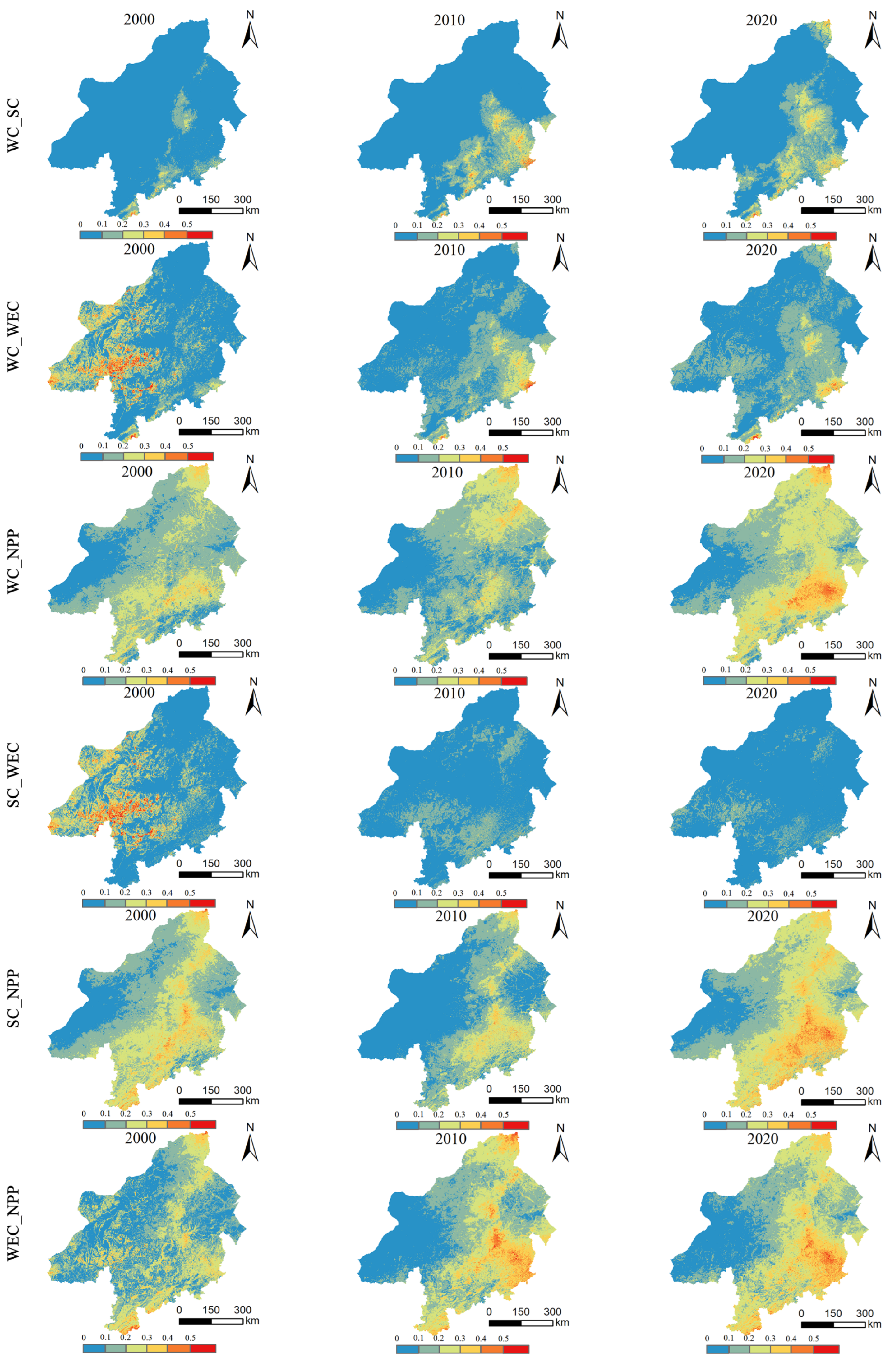
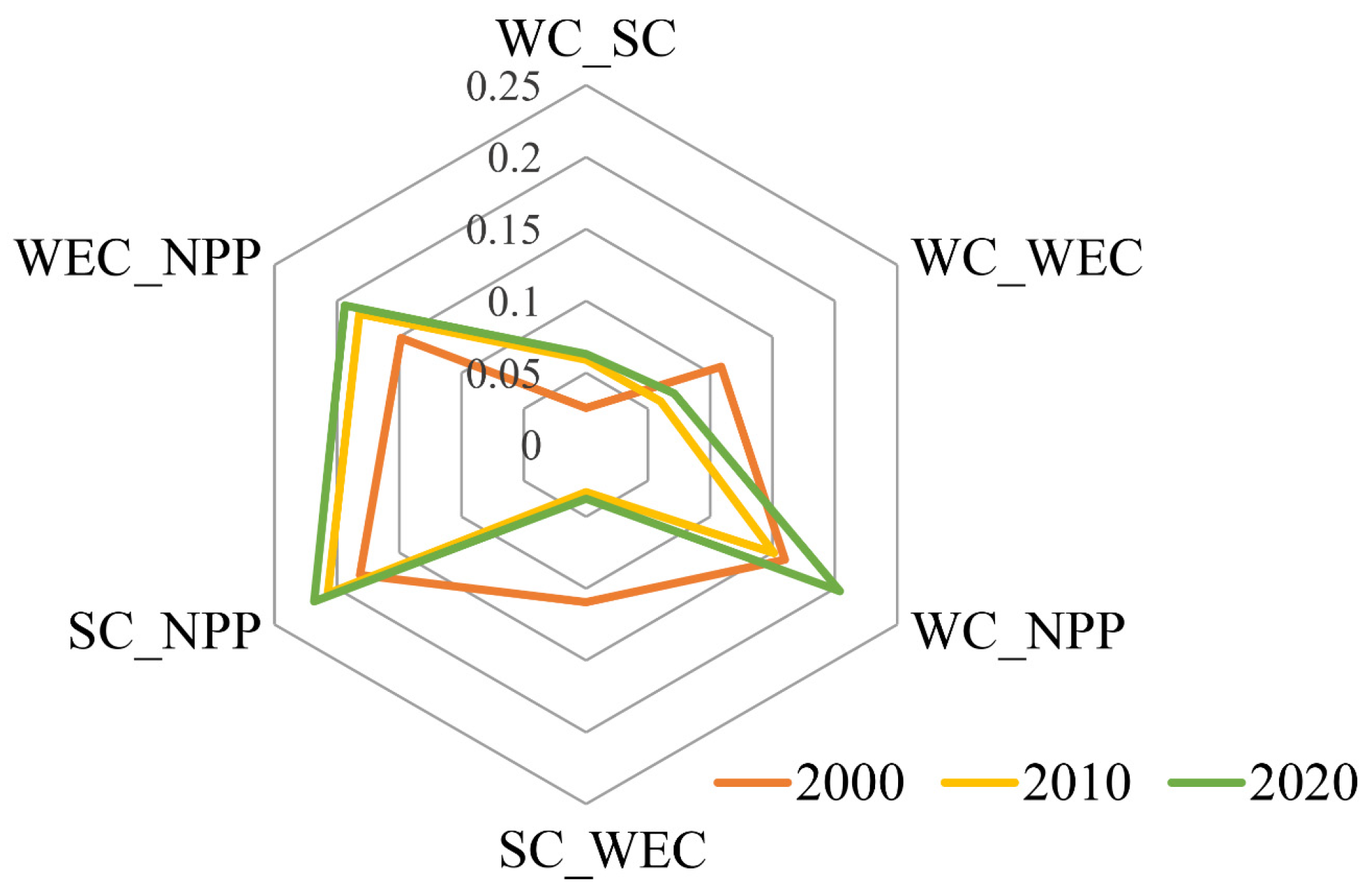
The RMSE was used to measure and spatially map the intensity of the trade-offs among the ecosystem services (Figure 3 and Figure 4). The RMSE of WC_SC increased by 0.039 since 2000. Its values were high in the central and southeastern regions, reflecting weak trade-offs. Moreover, there was an increase in trade-offs between WC and SC in this area since WC improved over the past two decades. The RMSE of WC_WEC decreased in the central and southern regions from 2000 to 2020 and increased in the southeastern part. The RMSE of WC_NPP was high (0.2–0.4), with the highest values (>0.4) concentrated in the northern and southeastern parts of the study area, where trade-offs were significant. The RMSE of WC_NPP increased significantly, by 0.044, in the BTSSCP during the study period. A relatively high value of the RMSE of SC_WEC was observed mainly in the western and southern regions. The overall RMSE of SC_WEC decreased by 0.072, which means that the trade-offs between SC and WEC had weakened. SC_NPP had a large RMSE (0.2–0.4), where the high-value areas were mainly located in the southeast of the study area. The RMSE of NPP increased by 0.037, indicating that trade-offs had been enhanced in the study area over the past 20 years. WEC_NPP recorded a large RMSE, which had increased by 0.046 from 2000 to 2020. High-value areas were concentrated in the southwest and southeast of the study area and reflected strong trade-offs.

3.3. Construction and Validation of the BBN

Following parametric learning, the BBN was able to represent prior probabilities of the status of the study area. According to the process mechanism of ecosystem services, the relevant variables in each ecological process in 2020 were selected as nodes to learn the structure of the Bayesian network. As shown in Figure 5, the constructed Bayesian conceptual network contained 15 nodes and 34 arrows. Six types of trade-off intensities were the target nodes, and nine variables (such as population density, slope, precipitation, land use, temperature, NDVI, wind speed, evapotranspiration, and GDP) were the influencing factors nodes. The probabilities of the four states (Low, Medium, High, and Highest) in terms of the WC_SC were weighed from low to high as 49.8%, 26.0%, 17.4%, and 6.77%. Those of WC_WEC from low to high were 43.6%, 29.8%, 17.8%, and 8.82%. The probabilities of the WC_NPP were 22.8%, 33.2%, 32.6%, and 11.4%, while the states of the SC_WEC had probabilities of 45.6%, 25.7%, 17.0%, and 11.7%. The probabilities of the states in terms of the SC_NPP were 19.3%, 33.7%, 33.1%, and 13.9%, while those in terms of the WEC_NPP were 18.3%, 35.2%, 31.7%, and 14.9%.
We tested the accuracy of the Bayesian network as well. To this end, we generated sampling points at 5 km intervals in the study area. A total of 18,281 sampling points were thus obtained. The tested nodes were six groups of ecosystem service trade-offs. We chose four parameters commonly used to assess the quality of a Bayesian network: the error rate, logarithmic loss, quadratic loss, and spherical payoff. They can reflect the magnitude of the error between the actual and predicted values of the target node [48]. The results show that the BBN was accurate (Table 4). This proves that the model could adequately represent ecosystem services and infer the nodal probabilities.

3.4. Spatial Optimization of Ecosystem Services

3.4.1. Sensitivity Analysis

The manner in which an observation at one node influences another node is a main concern in Bayesian networks [49]. We calculated the sensitivity index to quantify the contribution of each influential factor to ecosystem service trade-off. To determine the critical nodes (VR > 1%), we used the built-in function of the model to perform a sensitivity analysis on the driving variables. Table 5 shows the WEC, indicating that the precipitation, land use, and slope were the three most important nodes for WC_SC, of which precipitation had the highest VR value of 37% and thus the greatest impact on ecosystem service trade-off. Several factors influenced the ecosystem service trade-off of WC_WEC, including rainfall, evapotranspiration, and wind speed. Precipitation, NDVI, and temperature are known to be strongly correlated with WC_NPP trade-offs. Wind speed, precipitation, and atmospheric temperature had the greatest influence on the synergistic trade-off relationship of SC_WEC. The values of VR of the three nodes dominated by climatic factors reflected this trade-off relationship. The trade-offs in SC_NPP was influenced by the NDVI, precipitation, and land use. The value of VR of NDVI was 15.9%; thus, it had the most significant influence on the trade-offs. The NDVI is commonly used to measure vegetation cover across a given region. Vegetation cover also enhances the NPP. The NDVI, precipitation, and wind speed were found to influence the WEC_NPP trade-off.

3.4.2. Spatial Optimization of Ecosystem Services

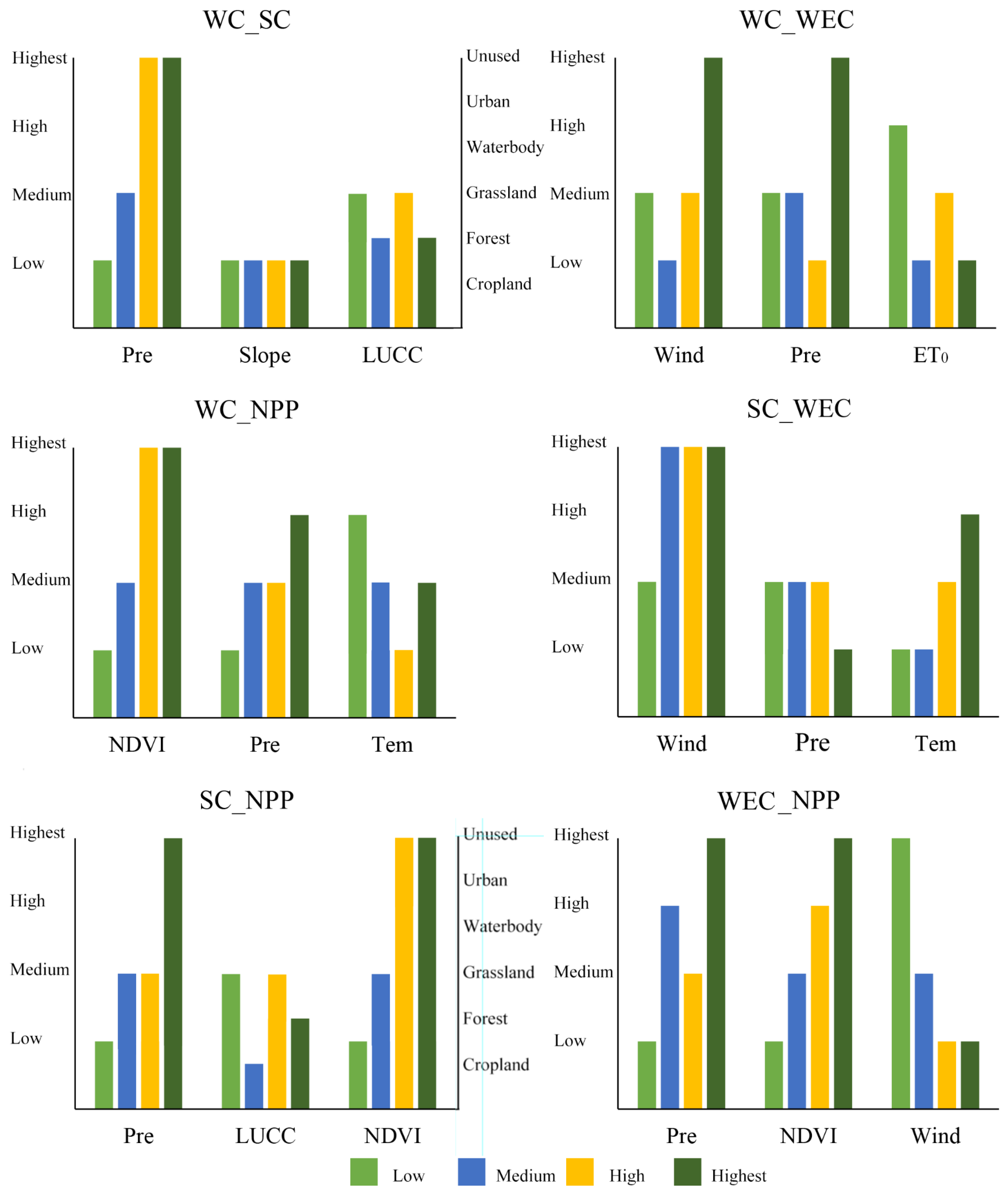
Figure 6 shows that three key variables that influenced the strength of trade-offs for different ecosystem services. For example, in the case of WC_SC: precipitation, slope, and land use. Their values varied according to whether the trade-offs were Low, Medium, High, or Highest (Table S2).
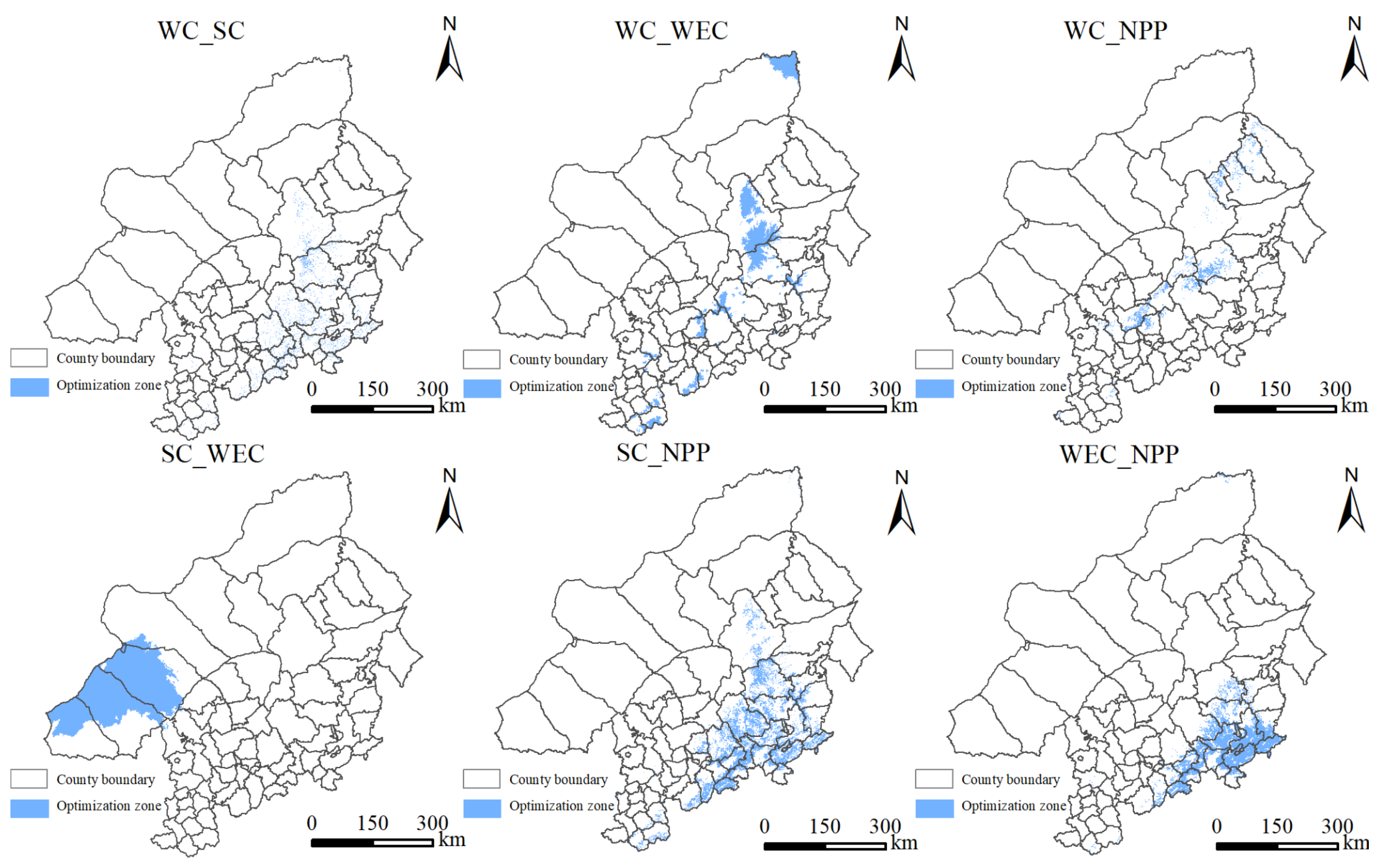
The conditional probability associated with the state of each variable can be expressed by the elemental layers within each subset of ecosystem services. Areas of optimization under the BTSSCP can be identified by analyzing the distributions of the key variables under different trade-off-related conditions (Figure 7).
The strength of the WC_SC trade-off was highest when the land use type was forest, precipitation was maximum, and slope had low value. Optimized zones were scattered in the central part of the country. When precipitation and wind speed were in the highest interval and evapotranspiration was in the low value area, the strength of the WC_WEC trade-off relationship reached its highest level, and the optimized area showed a faceted main distribution in Keshiketeng Banner and East Ujimqin Banner. The strength of the WC_NPP trade-off relationship reached its maximum when the precipitation was high, the NDVI was in the highest range, and the temperature was moderate, and the optimized areas were concentrated in the southern part of Weichang County and the northern part of Zhangbei County in the study area. The strength of the SC_WEC trade-off relationship was highest when the wind speed was in the medium interval, the precipitation was in the minimum range, and the temperature was high; this mainly occurred in the Sonid Left Banner, Sonid Right Banner, the north-central part of Siziwang Banner, and the northern part of the Darhan Muminggan Joint Banner. The intensity of the SC_NPP trade-off was most likely to be the highest when the land use type was forested and both precipitation and NDVI were in the highest range, and this occurred mainly in the southeastern part of the study area, including the northern parts of Beijing, Chengde, and Zhangjiakou. The WEC_NPP trade-off strength was maximized when the precipitation and NDVI were the highest and the wind speed was low. The optimized area included Kuancheng and Manzu County, located in the eastern part of the Yanshan mountain water conservation area. It also included southern Pingshuan County, Chengde County, Xinglong County, Luanping County, Huairou District, Yanqing District, Changping District, and Mentougou District.

4. Discussion

4.1. Interactions among Ecosystem Services

The results show that the four ecosystem services displayed different spatial distribution and change characteristics in the BTSSCP, similar to the research results of Xing et al. [50]. WEC had a trade-off relationship with SC and NPP, primarily because areas with high values of SC and NPP were largely concentrated in the southeastern part of the country. The terrain there is highly undulating, and areas with a high potential for wind erosion include the western region of desertification control, with a gentler terrain. This shows that WEC areas with potential for wind erosion and topographic relief were spatially heterogeneous. WEC was the main service provided by this area while the other ecosystem services were scarce [29,51].
We assessed the spatiotemporal trade-offs between ecosystem services using correlation coefficients and the RMSE. During the 2000–2020 period, the restoration of vegetation in the south-east regions enhanced the trade-off relationship between NPP, SC, WC, and WES, and decreased between WES, SC, and WC in the southwest. The south-east regions are located in the Taihang–Yanshan Ecological Conservation Area. Afforestation is the main type of restoration in this area, which may lead to an increase in the trade-off between ecosystem services. However, the main type of land use of the south-east area is grassland, and the restoration of grassland does not lead to higher trade-offs in ecosystem services.

4.2. Mechanisms Driving Ecosystem Service Trade-Offs

Ecosystem service trade-offs are often influenced by climatic conditions, land use, topography, and socio-economic development [52,53]. The results of the sensitivity analysis and probabilistic reasoning showed that precipitation, land use, NDVI, and temperature most significantly influenced the trade-off relationships. The results of our study are consistent with similar studies carried out in other areas. Zuo and Gao indicated that the determinants of the spatial trade-offs between erosion control and water yield, erosion control and carbon sequestration, and water yield and carbon sequestration were potential evapotranspiration, precipitation, and temperature, respectively [17]; Sun et al. revealed that climate was a critical factor in the provision of ecosystem services and their interactions [52]. Precipitation was the most significant factor influencing the trade-off relationship between ecosystem services. The patterns of land use in the BTSSCP have also drastically changed in the past 20 years. The aim of the Three Northern Protected Forest Restoration Project is the regulation of desertification through afforestation, whereas the Grain for Green Program aims for ecological conservation through the conversion of farmland and barren hillsides to forests [54,55,56]. The establishment of these projects has undoubtedly improved the vegetation cover of the BTSSCP and has considerably increased the capacity of vegetation NPP [57]. These ecological projects play crucial roles in land use changes, especially in terms of the reduction in the area cultivated land and the increase in the areas of forests and grasslands [50]. The NDVI of the central and eastern mountainous areas has increased by 15.8%, and this is significantly higher than in other regions, and has improved the NPP and SC while influencing the trade-off relationship between ecosystem services. In summary, owing to the poor socioeconomic development of the area and its low population density, the GDP has not had a significant impact on changes in regional ecosystem service relationships, while natural factors such as the climate and topography have had a more significant impact.

4.3. Limitations of the Model

We used a Bayesian network to identify the key factors influencing ecosystem service trade-offs, but its results are limited by uncertainty [25,58]. A greater number of influential factors should be considered in future work in the area. The hierarchical method of considering continuous variables can also introduce uncertainty to the parameter settings; thus, a more accurate dynamic method should be used to classify the node-related variables [59]. Although the model was validated for accuracy in the present research, the BBN model can be validated, and its accuracy can be improved using an uncertainty analysis in subsequent research to complete the improvement of the model.

4.4. Implications for Future Ecosystem Management

Ecosystem service trade-offs between the SC and WEC are largely distributed in the western part of the study area, which have low rainfall, high wind speeds, and moderate slopes. The SC is lower than in other regions. Therefore, ecological protection should be strengthened in this area and improve the SC on sloping lands. On the other hand, the southeastern areas with high trade-off values for the NPP, WC, SC, and WES should focus on water conservation in mountainous areas and reducing soil and wind erosion. This study suggests that relevant departments should implement ecological protection measures in the ecosystem service trade-off and synergistic optimization of the area, as well as pay attention to key drivers such as precipitation, NDVI, land use, and temperature when formulating relevant policies, so as to improve the local microclimate, enhance the quality of ecosystem services in the region, and promote the sustainable ecological and economic development of the study area.

5. Conclusions

The ecosystem service trade-offs of the BTSSCP have exhibited a strong spatial heterogeneity over the past 20 years. The spatial patterns of the WC and SC showed a distribution of “high values in the east and low values in the west,” while the NPP and WEC had a dispersed spatial distribution. The intensity of trade-offs involving the WC, SC, and NPP exhibited an upward trend while that of the other ecosystem services decreased. Several factors were found to have a significant impact on the intensity of the ecosystem service trade-offs within the study area, including precipitation, NDVI, types of land use, and temperature.
Based on the conditional probabilities of the key variables, the trade-off index between SC_WECs reached its maximum value when the wind speed was at its highest level, precipitation was at a low level, and temperature was higher. The optimized area was mainly located in the southwestern part of the study area when NDVI and precipitation were at the highest level and the land use type was a forest. The optimized areas were mainly located in the Yanshan mountain water conservation area, including Chengde, Zhangjiakou, and northern Beijing.

Supplementary Materials

The following supporting information can be downloaded at: https://www.mdpi.com/article/10.3390/su16041617/s1, Table S1: List of the method, model, software and parameters; Table S2: Conditional probability table for ecosystem service trade-off relationship.

Author Contributions

Conceptualization, J.L. and W.B.; Data Curation, J.L. and W.B.; Software, J.L.; Methodology, J.L. and W.B.; Formal Analysis, J.L.; Funding Acquisition, W.B.; Visualization, J.L.; Supervision, W.B., M.C., Q.C. and Y.L.; Validation, J.L. and W.B.; Project Administration, M.C, Y.L. and W.B.; Writing—Original Draft Preparation, J.L.; Writing—Review and Editing, W.B., M.C. and Y.L.; Resources, W.B.; Investigation, J.L. All authors have read and agreed to the published version of the manuscript.

Funding

This research was funded by the Special Fund of Chinese Central Government for Basic Scientific Research Operations in Commonweal Research Institutes (No. CAFYBB2020SY032); and the Chengde National Sustainable Development Agenda Innovation Demonstration Zone Construction Science and Technology Special Project: Research and Demonstration of Key Technologies for Integrated Ecological Protection and Restoration in the Upper Xiaoluan River (No. 202008F014).

Institutional Review Board Statement

Not applicable.

Informed Consent Statement

Not applicable.

Data Availability Statement

The data that support the findings of this study are available from the authors upon reasonable request.

Acknowledgments

All authors are grateful to the anonymous reviewers and editors for their constructive comments on earlier versions of the manuscript and acknowledge the data support from “National Earth System Science Data Center, National Science & Technology Infrastructure of China. (http://www.geodata.cn accessed on 25 July 2023)”.

Conflicts of Interest

The authors declare no conflicts of interest.

References

  1. Costanza, R.; D’arge, R.C.; Groot, R.D.; Farber, S.B.; Grasso, M.; Hannon, B.M.; Limburg, K.E.; Naeem, S.; O’Neill, R.V.; Paruelo, J.M.; et al. The value of ecosystem services: Putting the issues in perspective. Ecol. Econ. 1998, 25, 67–72. [Google Scholar] [CrossRef]
  2. Millennium Ecosystem Assessment. Ecosystems and Human Well-Being; Island Press: Washington, DC, USA, 2005. [Google Scholar]
  3. Fu, B.; Zhang, L. Land-use change and ecosystem services: Concepts, methods and progress. Prog. Phys. Geogr. 2014, 33, 441–446. [Google Scholar] [CrossRef]
  4. Costanza, R.; Groot, R.D.; Braat, L.C.; Kubiszewski, I.; Fioramonti, L.; Sutton, P.C.; Farber, S.B.; Grasso, M. Twenty years of ecosystem services: How far have we come and how far do we still need to go? Ecosyst Serv. 2017, 28, 1–16. [Google Scholar] [CrossRef]
  5. Wang, P.; Zhang, L.; Li, Y.; Jiao, L.; Wang, H.; Yan, J.; Lu, Y.; Fu, B. Spatio-temporal characteristics of the trade-off and synergy relationships among multiple ecosystem services in the Upper Reaches of Hanjiang River Basin. Acta Geogr. Sin. 2017, 72, 2064–2078. [Google Scholar] [CrossRef]
  6. Rodríguez, J.P.; Beard, T.D.; Bennett, E.M.; Cumming, G.S.; Cork, S.J.; Agard, J.; Dobson, A.P.; Peterson, G.D. Trade-offs across Space, Time, and Ecosystem services. Ecol. Soc. 2006, 11, 709–723. [Google Scholar] [CrossRef]
  7. Yi, F.; Yang, Q.; Wang, Z.; Li, Y.; Cheng, L.; Yao, B.; Lu, Q. Changes in Land Use and Ecosystem Service Values of Dunhuang Oasis from 1990 to 2030. Remote Sens. 2023, 15, 564. [Google Scholar] [CrossRef]
  8. Howe, C.; Suich, H.; Vira, B.; Mace, G.M. Creating win-wins from trade-offs? Ecosystem services for human well-being: A meta-analysis of ecosystem service trade-offs and synergies in the real world. Glob. Environ. Change 2014, 28, 263–275. [Google Scholar] [CrossRef]
  9. Su, B.; Liu, M. An ecosystem service trade-off management framework based on key ecosystem services. Ecol. Indic. 2023, 154. [Google Scholar] [CrossRef]
  10. Qi, X.; Li, Q.; Yue, Y.; Liao, C.; Zhai, L.; Zhang, X.; Wang, K.; Zhang, C.; Zhang, M.; Xiong, Y. Rural-Urban Migration and Conservation Drive the Ecosystem Services Improvement in China Karst: A Case Study of Huan Jiang County, Guangxi. Remote Sens. 2021, 13, 566. [Google Scholar] [CrossRef]
  11. Bennett, E.; Peterson, G.; Gordon, L. Understanding relationships among multiple ecosystem services. Ecol. Lett. 2009, 12, 1394–1404. [Google Scholar] [CrossRef]
  12. Obiang Ndong, G.; Therond, O.; Cousin, I. Analysis of relationships between ecosystem services: A generic classification and review of the literature. Ecosyst. Serv. 2020, 43, 101120. [Google Scholar] [CrossRef]
  13. Nelson, E.J.; Mendoza, G.F.; Regetz, J.; Polasky, S.; Tallis, H.; Cameron, D.R.; Chan, K.M.; Daily, G.C.; Goldstein, J.H.; Kareiva, P.; et al. Modeling multiple ecosystem services, biodiversity conservation, commodity production, and tradeoffs at landscape scales. Front. Ecol. Environ. 2009, 7, 4–11. [Google Scholar] [CrossRef]
  14. Chen, T.; Feng, Z.; Zhao, H.; Wu, K. Identification of Ecosystem Service Bundles and Driving Factors in Beijing and its Surrounding Areas. Sci. Total Environ. 2019, 711, 134687. [Google Scholar] [CrossRef] [PubMed]
  15. He, L.; Zheng, B.; Wan, W.; Xie, Z.; Song, X.; Zhu, J.; Liu, Z. Trade-off and Synergy of Ecosystem Services in the Yangtze River Economic Belt and Its Driving Factors. Chin. J. Environ. Sci. 2023. [Google Scholar]
  16. Lyu, R.; Clarke, K.C.; Zhang, J.; Feng, J.; Jia, X.; Li, J. Spatial correlations among ecosystem services and their socio-ecological driving factors: A case study in the city belt along the Yellow River in Ningxia, China. Appl. Geogr. 2019, 108, 64–73. [Google Scholar] [CrossRef]
  17. Zuo, L.; Gao, J. Investigating the compounding effects of environmental factors on ecosystem services relationships for Ecological Conservation Red Line areas. Land Degrad. Dev. 2021, 32, 4609–4623. [Google Scholar] [CrossRef]
  18. Feng, Z.; Jin, X.; Chen, T.; Wu, J. Understanding trade-offs and synergies of ecosystem services to support the decision-making in the Beijing-Tianjin-Hebei region. Land Use Policy 2021, 106. [Google Scholar] [CrossRef]
  19. Dade, M.C.; Mitchell, M.G.; McAlpine, C.A.; Rhodes, J.R. Assessing ecosystem service trade-offs and synergies: The need for a more mechanistic approach. Ambio 2019, 48, 1116–1128. [Google Scholar] [CrossRef]
  20. Frizzle, C.; Fournier, R.A.; Trudel, M.; Luther, J.E. Towards sustainable forestry: Using a spatial Bayesian belief network to quantify trade-offs among forest-related ecosystem services. J. Environ. Manag. 2021, 301, 113817. [Google Scholar] [CrossRef]
  21. Peng, L.; Chen, T.; Deng, W.; Liu, Y. Exploring ecosystem services trade-offs using the Bayesian belief network model for ecological restoration decision-making: A case study in Guizhou Province, China. Ecol. Indic. 2022, 48, 1116–1128. [Google Scholar] [CrossRef]
  22. Liu, Y.; Yuan, X.; Li, J.; Qian, K.; Yan, W.; Yang, X.; Ma, X. Trade-offs and synergistic relationships of ecosystem services under land use change in Xinjiang from 1990 to 2020: A Bayesian network analysis. Sci. Total Environ. 2023, 858, 160015. [Google Scholar] [CrossRef]
  23. Gonzalez-Redin, J.; Luque, S.; Poggio, L.; Smith, R.; Gimona, A. Spatial Bayesian belief networks as a planning decision tool for mapping ecosystem services trade-offs on forested landscapes. Environ. Res. 2016, 144 Pt B, 15–26. [Google Scholar] [CrossRef]
  24. Hobbs, N.T.; Hooten, M.B. Simple Bayesian Models; Princeton University Press: Princeton, NJ, USA, 2015. [Google Scholar] [CrossRef]
  25. Chen, S.; Pollino, C.A. Good practice in Bayesian network modelling. Environ. Model. Softw. 2012, 37, 134–145. [Google Scholar] [CrossRef]
  26. Liu, T.; Li, Z. Benefit Analysis on Beijing-Tianjin Sandstorm Sources Control Project in Ten Years; China Forestry Publishing House: Beijing, China, 2010. [Google Scholar]
  27. Liu, B.; Zhang, L.; Lu, F.; Deng, L.; Zhao, H.; Luo, Y.; Liu, X.; Zhang, K.; Wang, X.; Liu, W.; et al. Greenhouse gas emissions and net carbon sequestration of the Beijing-Tianjin Sand Source Control Project in China. J. Clean. Prod. 2019, 225, 163–172. [Google Scholar] [CrossRef]
  28. Wang, S.; Zhang, B.; Xie, G.; Zhai, X.; Sun, H. Vegetation cover changes and sand-fixing service responses in the Beijing-Tianjin sandstorm source control project area. Environ. Dev. 2020, 34, 100455. [Google Scholar] [CrossRef]
  29. Dai, L.; Tang, H.; Zhang, Q.; Cui, F. The trade-off and synergistic relationship among ecosystem services: A case study in Duolun County, the agropastoral ecotone of Northern China. Acta Ecol. Sin. 2020, 40, 2863–2876. [Google Scholar] [CrossRef]
  30. McKinley, G.A.; Fay, A.R.; Takahashi, T.; Metzl, N. Convergence of atmospheric and North Atlantic carbon dioxide trends on multidecadal timescales. Nat. Geosci. 2011, 4, 606–610. [Google Scholar] [CrossRef]
  31. Zhang, B.; Wang, S.; Li, Q.; Xie, G. Spatio-temporal changes of water conservation service in the Beijing-Tianjin sandstorm source control project area. Acta Ecol. Sin. 2021, 41, 7530–7541. [Google Scholar] [CrossRef]
  32. Yu, H.; Chen, J.; Zhang, Q. Characteristic Analysis of Ecological Water Use in Xilin River Basin Based on Remote Sensing. J. Risk Anal. Crisis Response 2018, 8, 216–222. [Google Scholar] [CrossRef]
  33. Lu, C.; Zhao, T.; Shi, X.; Cao, S. Ecological restoration by afforestation may increase groundwater depth and create potentially large ecological and water opportunity costs in arid and semiarid China. J. Clean. Prod. 2018, 176, 1213–1222. [Google Scholar] [CrossRef]
  34. Wang, S.; Zhang, B.; Shi, Y.; Xie, G.; Wu, Y.; Zhu, M. Exploring the combination and heterogeneity of ecosystem services bundles in the Beijing-Tianjin Sandstorm Source Control Project. Ecol. Indic. 2023, 155. [Google Scholar] [CrossRef]
  35. Hu, P.; Zhang, W.; Chen, H.; Li, D.; Zhao, Y.; Zhao, J.; Xiao, J.; Wu, F.; He, X.; Luo, Y.; et al. Soil carbon accumulation with increasing temperature under both managed and natural vegetation restoration in calcareous soils. Sci. Total Environ. 2021, 767. [Google Scholar] [CrossRef]
  36. Wang, S.; Zhang, B.; Wang, S.; Xie, G. Dynamic changes in water conservation in the Beijing–Tianjin Sandstorm Source Control Project Area: A case study of Xilin Gol League in China. J. Clean. Prod. 2021, 293. [Google Scholar] [CrossRef]
  37. Bao, Z.; Zhang, J.; Wang, G.; Chen, Q.; Guan, T.; Yan, X.; Liu, C.; Liu, J.; Wang, J. The impact of climate variability and land use/cover change on the water balance in the Middle Yellow River Basin, China. J. Hydrol. 2019, 577, 123942. [Google Scholar] [CrossRef]
  38. Ouyang, Z.Y.; ZHENG, H.; Xiao, Y.; Polasky, S.; Liu, J.; Xu, W.; Wang, Q.; Zhang, L.; Xiao, Y.; Rao, E.; et al. Improvements in ecosystem services from investments in natural capital. Science 2016, 352, 1455–1459. [Google Scholar] [CrossRef] [PubMed]
  39. Feng, T.; Chen, H.S.; Polyakov, V.O. Soil erosion rates in two karst peak-cluster depression basins of northwest Guangxi, China: Comparison of the RUSLE model with 137Cs measurements. Geomorphology 2016, 253, 217–224. [Google Scholar] [CrossRef]
  40. Wischmeier, W.H.; Smith, D.D. Predicting Rainfall Erosion Losses: A Guide to Conservation Planning; USDA: Washington, DC, USA, 1978.
  41. Melillo, J.M.; McGuire, A.D.; Kicklighter, D.W.; Moore, B.; Vorosmarty, C.J.; Schloss, A.L. Global climate change and terrestrial net primary production. Nature 1993, 363, 234–240. [Google Scholar] [CrossRef]
  42. Yu, D.; Shi, P.; Shao, H.; Zhu, W.; Pan, Y. Modelling net primary productivity of terrestrial ecosystems in East Asia based on an improved CASA ecosystem model. Int. J. Remote Sens. 2009, 30, 4851–4866. [Google Scholar] [CrossRef]
  43. Zhu, W.; Chen, Y.; Xu, D.; Li, J. Advances in terrestrial net primary productivity (NPP) estimation models. Chin. J. Ecol. 2005, 24, 296–300. [Google Scholar] [CrossRef]
  44. Pearl, J. Fusion, propagation, and structuring in belief networks. Artif. Intell. 1986, 29, 241–288. [Google Scholar] [CrossRef]
  45. Zhu, W.; Gao, Y.; Zhang, H.; Liu, L. Optimization of the land use pattern in Horqin Sandy Land by using the CLUMondo model and Bayesian belief network. Sci. Total Environ. 2020, 739, 139929. [Google Scholar] [CrossRef]
  46. MacPherson, M.P.; Webb, E.B.; Raedeke, A.H. A review of Bayesian belief network models as decision-support tools for wetland conservation: Are water birds potential umbrella taxa? Biol. Conserv. 2018, 226, 215–223. [Google Scholar] [CrossRef]
  47. Zheng, T.; Chen, S.; Zhang, T.; Xu, L.; Ma, L. Research on driving mechanism of ecological land loss based on Bayesian network. J. Nat. Resour. 2020, 35, 2980–2994. [Google Scholar] [CrossRef]
  48. Kalacska, M.; Sánchez-Azofeifa, G.A.; Calvo-Alvarado, J.C.; Rivard, B.; Quesada, M. Effects of Season and Successional Stage on Leaf Area Index and Spectral Vegetation Indices in Three Mesoamerican Tropical Dry Forests. Biotropica 2005, 37, 486–496. [Google Scholar] [CrossRef]
  49. Li, X.Y.; Zhang, L.; Zhang, S. Efficient Bayesian networks for slope safety evaluation with large quantity monitoring information. Geosci. Front. 2018, 9, 9. [Google Scholar] [CrossRef]
  50. Xing, X.; Yang, X.; Guo, J.; Chen, A.; Zhang, M.; Yang, D.; Hou, Z.; Zhang, H.; Wang, X. Response of ecosystem services in Beijing-Tianjin Sandstorm Source Control Project to differing engineering measures scenarios. J. Clean. Prod. 2023, 384, 135574. [Google Scholar] [CrossRef]
  51. Jiang, C.; Zhang, H.; Zhang, Z.; Wang, D. Model-based assessment soil loss by wind and water erosion in China’s Loess Plateau: Dynamic change, conservation effectiveness, and strategies for sustainable restoration. Glob. Planet Change 2019, 172, 396–413. [Google Scholar] [CrossRef]
  52. Sun, X.; Ye, D.; Shan, R.; Peng, Q.; Zhao, Z.; Sun, J. Effect of physical geographic and socioeconomic processes on interactions among ecosystem services based on machine learning. J. Clean. Prod. 2022, 20, 359. [Google Scholar] [CrossRef]
  53. Li, C.; Zhao, J.; Zhuang, Z.; Gu, S. Spatiotemporal dynamics and influencing factors of ecosystem service trade-offs in the Yangtze River Delta urban agglomeration. Acta Ecol. Sin. 2022, 42, 5708–5720. [Google Scholar] [CrossRef]
  54. Zhang, Y.; Peng, C.; Li, W.; Tian, L.; Zhu, Q.; Chen, H.; Fang, X.; Zhang, G.; Liu, G.; Mu, X. Multiple afforestation programs accelerate the greenness in the ‘Three North’ region of China from 1982 to 2013. Ecol. Indic. 2016, 61, 404–412. [Google Scholar] [CrossRef]
  55. Deng, L.; Liu, G.; Shangguan, Z.P. Land-use conversion and changing soil carbon stocks in China’s ‘Grain-for-Green’ Program: A synthesis. Glob. Change Biol. 2014, 20, 3544–3556. [Google Scholar] [CrossRef]
  56. Xu, S.; Su, Y.; Yan, W.; Liu, Y.; Wang, Y.; Li, J.; Qian, K.; Yang, X.; Ma, X. Influences of Ecological Restoration Programs on Ecosystem Services in Sandy Areas, Northern China. Remote Sens. 2023, 15, 3519. [Google Scholar] [CrossRef]
  57. Li, C.; Fu, B.; Wang, S.; Stringer, L.C.; Wang, Y.; Li, Z.; Liu, Y.; Zhou, W. Drivers and impacts of changes in China’s drylands. Nat. Rev. Earth Environ. 2021, 2, 858–873. [Google Scholar] [CrossRef]
  58. Peng, Y.; Zhang, S.; Pan, R. Bayesian Network Reasoning with Uncertain Evidences. J. Uncertain. Fuzziness Knowl.-Based Syst. 2010, 18, 539–564. [Google Scholar] [CrossRef]
  59. Xue, J.; Gui, D.; Lei, J.; Sun, H.; Zeng, F.; Feng, X. A hybrid Bayesian network approach for trade-offs between environmental flows and agricultural water using dynamic discretization. Adv. Water Resour. 2017, 110, 445–458. [Google Scholar] [CrossRef]
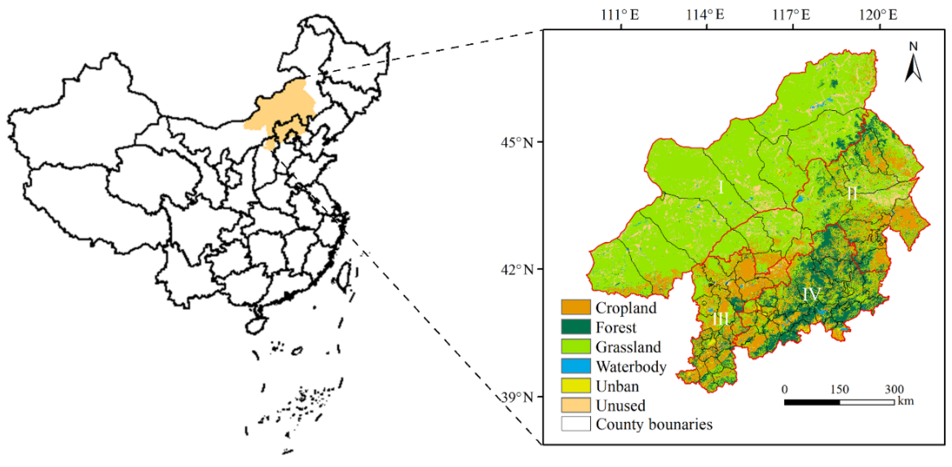
Figure 1. Geography of the study area and land use in 2020. Note: I. Sandy area with an arid grassland. II. Hunshandake sandy land. III. Psturage ecotone sandy land. IV. Yanshan mountain water conservation area.
Sustainability 16 01617 g001
Figure 2. Ecosystem services in the BTSSCP.
Sustainability 16 01617 g002
Figure 3. Spatial distribution of the RMSEs of the ecosystem services. Note: WC_SC: water conservation and soil conservation. WC_WEC: water conservation and wind erosion control. WC_NPP: water conservation and net primary productivity. SC_WEC: soil conservation and wind erosion control. SC_NPP: soil conservation and net primary productivity. WEC_NPP: wind erosion control and net primary productivity.
Sustainability 16 01617 g003
Figure 4. Radar chart of the RMSEs of the ecosystem services.
Sustainability 16 01617 g004
Figure 5. Bayesian network of the ecosystem services in the study area in 2020.
Sustainability 16 01617 g005
Figure 6. Plots of the conditional probabilities of the key variables.
Sustainability 16 01617 g006
Figure 7. Regional distribution of the areas of optimization of the BTSSCP.
Sustainability 16 01617 g007
Table 1. Sources of primary data.
Type of DataDescription of DataData Source
Land useIncluding cropland, forest, grassland, waters, construction, and unutilized land, with a spatial resolution of 30 mResource and Environmental Sciences Data Center, Chinese Academy of Sciences (https://www.resdc.cn/ accessed on 9 June 2023)
ElevationThe spatial resolution was 30 mGeospatial Data Cloud (https://www.gscloud.cn/ accessed on 18 July 2023)
MeteorologicalIncludes temperature, precipitation, and wind speed, with a spatial resolution of 1 km.National Earth System Science Data Center (http://www.geodata.cn/ accessed on 25 July 2023)
Data statisticsA raster dataset for 2000–2020 of population density and GDP at a spatial resolution of 1 kmData Center for Resource and Environmental Sciences, Chinese Academy of Sciences (https://www.resdc.cn/ accessed on 8 July 2023)
Soil dataContains sand, silt, clay, organic carbon, and soil organic carbon content at a 250 m resolutionSoilGrids250m.2.0
NDVI, NPPData for MOD13A3 and MOD17A3, with a spatial resolution of 1 km and 500 mNational Aeronautics and Space Administration
Table 2. The temporal changes of the four ecosystem services from 2000 to 2020.
Ecosystem Service 200020102020
WCTotal (m3)16.18 × 10820.43 × 10823.61 × 108
Average (mm)3.534.465.16
SCTotal (t)4.19 × 1084.51 × 1084.60 × 108
Average (t/hm2)9.159.8410.04
WECTotal (t)2.73 × 1092.84 × 1093.14 × 109
Average (t/hm2)59.6162.0268.57
NPPTotal (Tg)80.61102.14128.27
Average (gC·m−2)176223.01280.07
Table 3. Correlations among the ecosystem services in the study area.
Ecosystem ServiceYearSCWECNPP
WC20000.623 **0.031 **0.781 **
20100.607 *0.049 **0.759 **
20200.592 **0.046 **0.767 **
SC2000 −0.095 **0.644 **
2010 0.029 *0.626 **
2020 0.026 **0.61 **
WEC2000 −0.064 **
2010 −0.093 **
2020 −0.105 *
Note: ** and * represent significant correlations at 0.01 and 0.05.
Table 4. Assessment of BBN accuracy.
ParameterError RateLogarithmic LossQuadratic LossSpherical Payoff
WC_SC27.13%0.58440.35760.7897
WC_WEC36.94%0.79690.47580.7171
WC_NPP30.58%0.69160.40440.7606
SC_WEC39.27%0.88270.50150.6978
SC_NPP27.29%0.61560.36450.7887
WEC_NPP28.06%0.6370.37780.7809
Table 5. BNN sensitivity analysis.
WC_SCWC_WECWC_NPPSC_WECSC_NPPWEC_NPP
NodeVR/%NodeVR/%NodeVR/%NodeVR/%NodeVR/%NodeVR/%
Pre37Pre9.75NDVI14.9Wind1.6NDVI15.9NDVI6.93
Lucc2.09ET01.74Pre3.74Pre1.49Pre5.94Pre4.2
Slope1.67Wind1.5Tem1.55Tem1.21Lucc1.72Wind2.29
ET00.45NDVI0.85ET00.49Slope0.93Tem0.49Tem0.62
Tem0.41Tem0.33Lucc0.29ET00.44ET00.48ET00.47
Pop0.11Lucc0.29Pop0.02Lucc0.43Slope0.32Lucc0.28
GDP0.03Pop0.02GDP0NDVI0.25Pop0.03Pop0.01
NDVI0GDP0Slope0Pop0.04GDP0GDP0
Wind0Slope0Wind0GDP0.01Wind0Slope0
Note: “Pre”, “ET0”, “Tem”, “Pop”, “Wind”, “GDP’’, and “Lucc” refer to precipitation, evapotranspiration, temperature, population, wind speed, gross domestic product, and land use, respectively.
Disclaimer/Publisher’s Note: The statements, opinions and data contained in all publications are solely those of the individual author(s) and contributor(s) and not of MDPI and/or the editor(s). MDPI and/or the editor(s) disclaim responsibility for any injury to people or property resulting from any ideas, methods, instructions or products referred to in the content.