Mapping Urban Expansions along China–Europe Railway Express with the 30 m Time-Series Global Impervious Surface Area (GISA-2) Data from 2010 to 2019

Abstract

The China–Europe Railway Express (CRE) plays a crucial role in promoting local economic development and bolstering regional connectivity. Quantitative assessments of urban changes along the CRE are essential for understanding its influence on the local eco-environment and the economy, which is a cornerstone for fostering sustainable growth. Urban boundaries are vital indicators of city development; however, accurately extracting these boundaries over multiple years at a large scale and fine granularity remains challenging. On the basis of a global impervious surface area (GISA2) dataset from 2010 to 2019, this study extracted fine-scaled city boundaries annually for European countries and analyzed the spatiotemporal patterns of urbanization in areas along and not along the express during the past decade. The generated enhanced urban boundaries (EUBs) show strong agreement with the Landsat time-series data and align well with existing global urban time-series products (GUB, GAUD, and NTL). From 2010 to 2019, urban areas and clusters expanded across the entire region, with notable disparities observed between areas along the express (noted as ON-CRE) and those not along (noted as OFF-CRE). ON-CRE cities experienced more substantial urban growth near the express, resulting in new mega urban agglomerations and expansion in small and moderate cities. In contrast, most OFF-CRE cities exhibited stable development with limited urban sprawl. Dynamic proportions of the impervious surface area (ISA) within the EUB indicated more compact impervious areas within ON-CRE boundaries compared to OFF-CRE. This study contributes to understanding urban expansions driven by the long-term CRE operations. The EUB dataset developed herein provides a valuable resource for future investigations into the impacts of urbanization on biotic stress and urban health in European countries, thus supporting the achievement of sustainable development goals.

1. Introduction

The China–Europe Railway Express (CRE) represents an internationally joint railway transportation service based on fixed train numbers and lines, schedules, and whole-course operation hours between China and Europe and other Belt and Road Initiative (BRI) countries (http://www.china-railway.com.cn/english/InternationalCooperation/CRexpress/201904/t20190409_93060.html, accessed on 8 June 2023). As the flagship project of the BRI, the CRE has advantages in price, capacity, and security, thus becoming one of the most important transportation routes in promoting the trade between East and West, accelerating the development of economic globalization during the past ten years. The express network had achieved extensive coverage, spanning 174 cities across 23 European nations, with the operational train count surpassing 40,000 by the year 2020 (http://www.china-railway.com.cn accessed on 14 September 2021). Following a period of four years of sustained expansion, by November 2023, the express expanded to 217 cities in 25 European countries, with the total number of trains in operation exceeding 81,000 (http://www.china-railway.com.cn accessed on 6 December 2023), bringing a profound impact on market transaction and infrastructure construction.

Urban area constitutes the most concentrated area of human activities. Driven by economic, demographic, technological, and political factors, the rate and extent of urbanization vary considerably across countries and years, resulting in diverse spatiotemporal expansion characteristics [1,2,3]. European countries have experienced a significant urbanization trend over the past decade, yet the dynamic changes in regions along the CRE have been underexplored. Previous studies have largely focused on trade management, with limited attention paid to urbanization in CRE-adjacent regions [4,5,6,7]. Therefore, it is necessary to understand the difference in the evolution of urbanization patterns for regions along and not along the express, where the CRE impacted diversely, so as to provide planning implications for these countries and help in achieving the sustainable development goals.

As an important indicator of sustainable development, accurate and long-term urbanization change monitoring has been attracting enormous attention in the literature. Compared with field survey, satellite-based observation has the unique advantages of a fine revisit frequency and large-area coverage. Efforts have been devoted to mapping the dynamics of the urban extent at different scales with various satellite-based datasets. Artificial Nighttime Light (NTL) datasets derived from sensors, e.g., Defense Meteorological Satellite Program Operational Linescan System (DMSP-OLS) and the Suomi National Polar-orbiting Partnership satellite’s Visible Infrared Imaging Radiometer Suite (NPP/VIIRS), could provide explicit observations for artificial lighting sources at night, and have been proved to be efficient in delineating the potential extent of socio-economic development [8]. However, it has been reported the derived urban extent may be more closely related to locations where higher-intensity human activities locate [9]. This saturation phenomenon in urban cores will inversely result in a blooming effect, i.e., overestimation in suburban areas [10]. Due to the lack of onboard radiometric calibration, the problem remains challenging [11]. Optical satellite observations from Moderate Resolution Imaging Spectroradiometer (MODIS), Sentinel, Landsat, and high-resolution sensors are another main data source to obtain urban areas. Although explicit landcover types can be extracted with optical satellite datasets, the difference in the detecting strategy, spatial coverage, revisit cycles, and processing cost limit the sole dataset to consistently obtain accurate information on the urban extent dynamics over a long period.

Impervious surface areas (ISAs) are surfaces covered by impervious materials and generally include areas with low permeability, such as squares, roads, roofs, parking lots, and so on. The variation in impervious surfaces reflects cities’ socio-economic and urban development [12]. The ISA is crucial for biodiversity [13,14], water quality [15], urban heat island effects [16,17], and ecological environments [18,19]. The emergence of ISA products has provided new indicators for measuring human activity intensity and reflecting the urban development process [20]. Global ISA datasets, developed over the past two decades, such as the global artificial impervious area (GAIA) [21], global annual urban dynamics (GAUD) [22], global impervious surface area (GISA) [23], and global human settlement layer (GHSL) [24], have provided new metrics for human activity and urban growth. Although these datasets exhibited a similar ISA increasing trend, they were different in the ISA spatial distribution [25]. For example, these datasets show consistent results in urban core areas but relatively large discrepancies in suburban or rural areas, which are mainly due to differences in sampling, mapping methods, and even the satellite imagery used [26]. The newly developed 30 m global ISA dataset (GISA 2.0) considers the inconsistency of the existing products with a unique mapping division strategy [27], offering improved accuracy and reduced omission errors. For long time-series maps (i.e., GISA 2.0, GISA, GAIA, GAUD, and GHSL), GISA 2.0 has the highest overall accuracy at global, arid and rural, and city scales. Therefore, GISA 2.0 can be served as a baseline for global ISA maps [28]. In addition, it should be pointed out that the “urban extents” defined as core urban domains (generally derived from NTL and ISA) include most built-up areas and partially green spaces and other land-use types with urban functions. It is rather different from the “urban boundaries” in this study determined as the spatial distribution of the artificial impervious area, where small urban patches will be removed and inner non-urban areas will be filled [29]. Hence, the results from NTL and ISA products are no longer suitable for directly extracting the urban boundaries; therefore, it is immensely demanded to develop a new framework to obtain the large-scale urban boundaries continuously.

Cloud computing platforms like Google Earth Engine (GEE) have facilitated the rapid, automated mapping of vast land areas [30,31]. With the GEE cloud platform, we improved an automated urban boundary extraction scheme originally developed by Li [32], based on the GISA 2 dataset from 2010 to 2019, delineated fine-scaled city boundaries/expansions annually, and analyzed the spatiotemporal dynamics of urbanization in areas along and not along the CRE during the past decade (the period from 2010 to 2019, since the opening year of the CRE was 2010 and the latest year of GISA2 is 2019). Firstly, the urban fringe and initial boundaries were extracted using a combination of kernel density estimation (KDE) and morphological methods. Subsequently, a multiscale fusion strategy was introduced to optimize and refine the urban boundary results. We then produced annual urban boundary datasets for European regions within the study period and compared the urbanization patterns of areas influenced by the CRE.

The main contributions of this study are twofold: (1) to provide an annual, fine-scaled city boundaries/expansions dataset for the CRE region; and (2) to help understand the urban expansions driven by the CRE’s long-term operations, thereby contributing to the fulfillment of Sustainable Development Goal 15.

The remainder of this paper is organized as follows. In Section 2, we provide a brief introduction to the study area and datasets and describe the automated urban boundary extraction method. The experimental results for the urban boundaries are provided in Section 3. Section 4 discusses the consistency between our results and others derived from state-of-the art datasets. The last section concludes the paper with some remarks and hints at plausible future research lines.

2. Materials and Methods

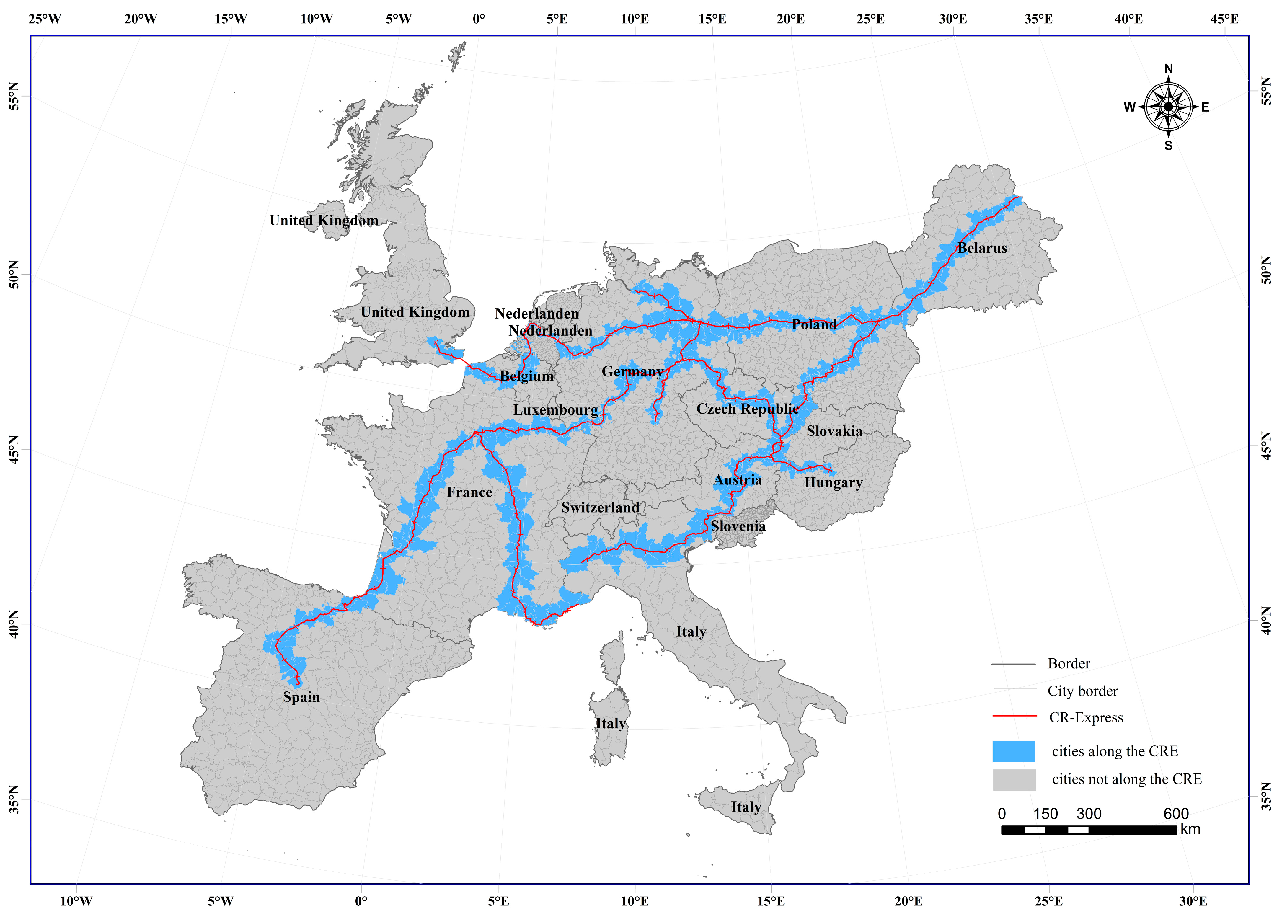
2.1. Study Area

We selected a total of 38 countries and regions in Europe (Figure 1) as our study area, and the study period extends from 2010 to 2019. The area covers a total administrative area of approximately 4 million km² and a total population of 500 million [33]. This area has diverse landscapes (e.g., deserts, mountains, and frozen areas), and heterogeneous geographical substratum, which pose extensive challenges for accurate landscape interpretation. Over the past decade, a markable expansion in the urban extents is reported as a result of the rapid growth in population and economy. The urban areas increased by an average of 1883 km² yr⁻¹ for the 1985–2015 period [22]. Meanwhile, uneven development patterns in those countries have also been noticed and figured out by Althouse [34] and Heiskanen [35], due to various local policies, environments, and socio-economic conditions.

In order to distinguish the varying influence of CRE establishment on local urban sprawling, according to the ”China-Europe Railway Express Development Report” [36], we divided the entire study area into two parts for the comparative analysis of the urban dynamics over the past decade: (1) areas along the express, which encompass 18 countries and regions, and (2) areas not along the express, which consist of 19 countries and regions, and their information is shown in

Table 1. Dividing the study area into along and not along the CRE (by July 2021).

(1) 18 Countries and Regions along the Express	(2) 19 Countries and Regions Not along the Express
Austria, Belarus, Belgium, Czech Republic, France, Germany, Hungary, Italy, Latvia, Lithuania, Luxembourg, Monaco, Netherlands, Poland, Serbia, Slovakia, Spain, United Kingdom.	Albania, Andorra, Bosnia and Herzegovina, Bulgaria, Croatia, Denmark, Estonia, Greece, Ireland, Liechtenstein, Moldova, Montenegro, North Macedonia, Portugal, Romania, San Marino, Slovenia, Switzerland, Vatican City.

. Analysis for the Russian Federation is not included due to the data availability.

2.2. Data

2.2.1. Global Impervious Surface Area (GISA 2)

The annual dynamics of the global impervious surface area (GISA 2) developed by Huang [27] were used for the modeling. Based on an integrated classification approach for global ISA mapping based on the spatial–temporal consistency of the existing products, the GISA 2 dataset has a 30 m spatial resolution and annual temporal resolution spanning from 1972 to 2019, which provides a high level of detail for urban boundary extraction and analysis and allows for an accurate assessment of the spatial dynamics of urbanization. These maps were generated with two special grid-based mapping strategies, which fully consider the inconsistency and consistency of the existing global ISA products, e.g., GAIA, GAUD, the first 10 m resolution global landcover map (FROM_GLC10) [37]. Overall accuracy for all maps is above 90%. Specifically, pixels in this dataset indicate the first year when the ISA was detected. Focusing on the data from 2010 to 2019, this study analyzed the long-term city expansion patterns before and after the establishment of the CRE, providing insights into the impact of the express on urbanization patterns in the region. Figure 2 depicts the overall GISA2 data and the ISA distribution of GISA2 in 2019.

2.2.2. CRE Outline Data and Other Ancillary Data

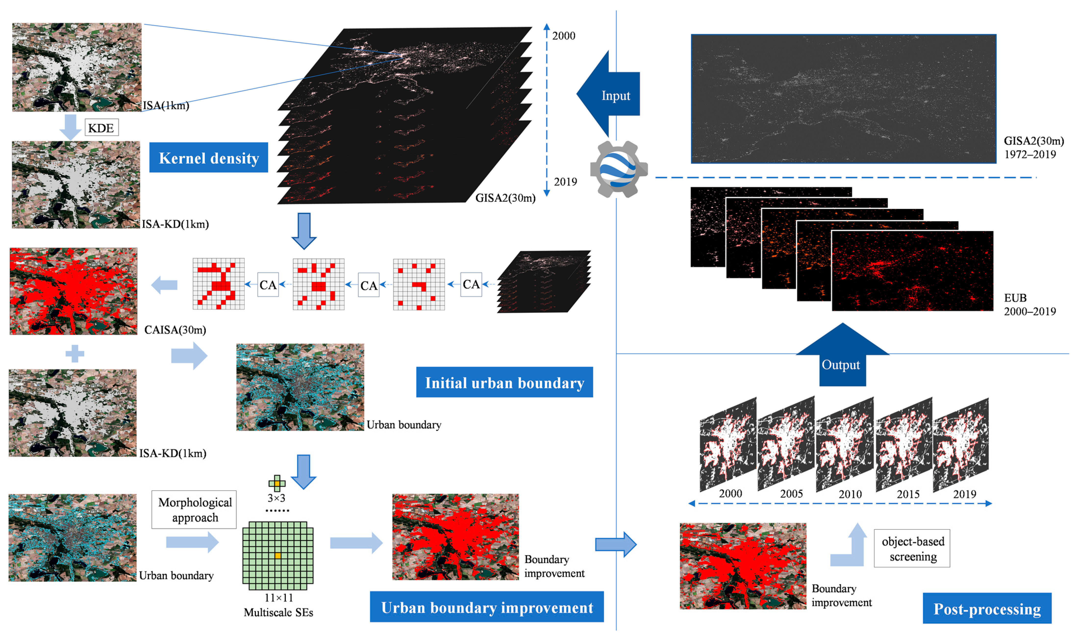
We used the Esri railway dataset as the preliminary dataset to manually trace and vectorize the CRE outline, with ancillary support provided by the railway dataset from “Natural Earth” at 10 m resolution to fill in missing information. Additionally, this CRE outline data were further verified through on-site field surveys based on Google Earth images collected from the 18 countries and regions along the express to ensure their accuracy and reliability (shown in Figure 1 with the red dot lines).

2.3. Methodology

We delineated the annual urban boundaries from 2010 to 2019 using GISA-2 product within a refined stepwise-partitioning framework (Figure 3), which essentially expands and enhances the urban mapping strategy created for the global urban boundary (GUB) [32]. The resulting urban boundaries are hereby referred to as enhanced urban boundaries (EUBs).

This scheme consists of three parts:

(1)

Initial boundary extraction: aggregation of ISA to delineate prospective urban fringes through a kernel density estimator;

(2)

Boundary improvement: multiscale fusion applied to refine the initial urban boundaries, which distinctively diverges from Li’s foundational framework [34] by offering an explicit spatial enhancement for cities of different scales;

(3)

Post-processing: measures designed to rectify minor discontinuities (e.g., small water bodies and green spaces) within the urban fabric and to ensure the temporal coherence of the urban expansion patterns.

These procedures were executed on the Google Earth Engine (GEE) platform, which provides massive remote sensing (RS) datasets and built-in image processing algorithms, thus enabling researchers to perform large-scale and long-term analyses with a substantially reduced cost and resources. Subsequent sections provide the details of the stepwise EUB mapping methodology.

2.3.1. Urban Fringe and Initial Boundary Extraction

We collected the long time-series GISA 2 dataset from https://zenodo.org/record/5136330 (accessed on 8 February 2023) and linked to the GEE platform. Annual GISA 2 results spanning from 2010 to 2019 were separated from the archived dataset, before the urban fringe and initial boundary extraction was performed using the kernel density estimation (KDE) aggregating and cellular automata (CA) method.

Firstly, we upscaled the 30 m resolution GISA-2 data to generate the ISA data annually, which refer to the percentage of urban areas within the 1 km grid. However, because the derived ISA results suffer from the heterogeneity of urban lands in central urban areas, we applied the kernel density (KD) with symmetric Gaussian point spread function to estimate the kernel density of each ISA pixel. The curved surface value of the specific point (ISA_c) was calculated as the sum of the weights of neighbor points (ISA_i) within a circular window as follows:

$$ISAKD\left(x\right)=\frac{1}{nh}{\displaystyle \sum _{i=1}^{n}K\left(\frac{IS{A}_c-IS{A}_i}{h}\right)}$$

(1)

where h denotes the size of the moving search window, and K is the KD function and determines the shape of the curved surface. We set the h as 5 × 5 (i.e., 25 km²), consistent with Zhao [38]. The data range for the obtained ISA-KD is [0, 1]. For pixels with values above 0.2, we determined their urbanization category in this year as “urban areas” [39].

However, due to the coarse resolution, some small urban patches in/around the city center will be missed in this step, even though most inner urban areas could be filled. In order to fill in the inner urban areas missed by the ISA-KD, we applied the CA-based model to the 30 m resolution GISA-2 data annually. Focusing on the self-evolution of the urban cell that is driven by its neighbors [40], urban CA models are mainly configured by the transition rules and neighborhoods.

The transition rules are calculated as a vector of transition potentials for each cell at each simulation using

$$\begin{array}{l}{P}_{suit}=\frac{1}{1+ex{p}^{-z}}\\ z=b_0+b_1{x}_1+\cdots +b_n{x}_n\end{array}$$

(2)

where P_suit is the transition potential, which determines the suitability of urban development, b₀ is the intercept parameter, b_i and x_i are the ith coefficient and spatial proxy.

N is the neighborhood effect on the cell:

$$N=\left(\frac{{{\displaystyle \sum }}_{{k,m,d}^{w_{kd}\times I_{md}}}}{d\times d-1}\right),I_{md}=\left\{\begin{array}{l}1,state of cell=k\hfill \\ 0,otherwise\hfill \end{array}\right.$$

(3)

where m is the index of the cells within the distance zone d, w_kd is the weighting parameter applied to the cells with state k (urban or not) in distance zone d, I_md is the conditional function and returns 1 when the status of the cell is urban.

The state of a pixel can be estimated according to its initial state P₀, the surrounding neighborhood effects N, and a set of transition rules P_suit.

$$P_{dev}=P_{suit}\times N\times P_0$$

(4)

where P_dev is the range of the target pixel, P_suit is the transition rules, P₀ is the initial state of a pixel, N represents the surrounding neighborhood effects.

In this step, we used a rectangular (Moore) neighborhood CA model (with d × d = 11 × 11 windows), and extracted pixels (with the percentage of urban pixels in the window above 20%) as urban areas, as suggested by Kocabas and Dragicevic [41]. The neighborhood effect can be measured by calculating the percentage of the urban cells in a 11 × 11 neighborhood. After 3 iterations, an approximate urban boundary noted by CA-ISA is generated with a total expansion distance of about 1 km (3 iterations × 11 pixels × 30 = 990 m), which is close to the spatial resolution of the ISA-KD (1 km). By combining the results from the CA-ISA (30 m) and the ISA-KD (1 km), we can obtain an initial urban boundary, which can cover most inner urban areas and well capture the spatial pattern of the urban extents.

2.3.2. Boundary Improvement with Multiscale Fusion

We improved the derived urban boundary around urban fringe areas using a morphological approach. Morphology is one of the most popular methods developed to explore the spatial information of the remote sensing data. The combinations of basic morphological operators (dilation and erosion) are known as opening and closing. Opening operations act on bright objects (urban pixels) compared with their surroundings (non-urban pixels), while closings act on dark objects. These operators are applied to an image with a set of known shapes, i.e., structuring elements (SEs). The size and shape are the key parameters of SEs, and objects where the SE does not fit will be deleted from the image. In contrast to classical morphological openings and closing, we chose morphological opening-by-reconstruction presented in Equation (5), which can solve the problem of over-reconstruction while preserving the shape of objects as much as possible [42,43], to improve the performance of urban boundary extraction.

$${\gamma }_I^{re}\left(d,s\right)=\left(I\Theta SE\left(d,s\right)\right)\oplus SE\left(d,s\right)\cap I$$

(5)

where ${\gamma }_I^{re}\left(d,s\right)$ represents the opening-by-reconstruction of the initial urban boundary I, and s and d indicate the length and direction of a linear SE, respectively. The symbols $⊝$ and $⨁$ are the morphological erosion and dilation operators.

Considering the heterogeneity of urban scales across European cities, a single SE is no longer suitable to precisely extract all the urban boundaries. Tiny cities will be missed with large SEs, whereas urban boundaries will be overestimated with small SEs. A multiscale strategy is employed to avoid these concerns based on different SEs and a range of increasing sizes of morphological operators. More specifically, we chose a series of line SEs (four directions are considered in this study, and size is determined as s_min = 3, s_max = 11, ∆s = 2) and sequentially implemented the opening-by-reconstruction to absorb those small urban patches into the final urban boundaries, and to remove isolated urban patches, simultaneously. The multiscale fusion rule is as follows:

$$\begin{array}{c}x\in Vote\left({\displaystyle \prod _{OBR}\left(I\right)}\right)\\ where{\displaystyle \prod _{OBR}\left(I\right)}=\left\{{\displaystyle \prod _{OBR}^{SE}\left(I\right)}\right\}=\left\{{\gamma }_I^{re}\left(d,s\right),\forall d=\left[45°,135°,225°,315°\right],s=\left[3,11\right]\right\}\end{array}$$

(6)

where OBR represents the opening-by-reconstruction and SE represents the structuring element. Four directions (45°, 135°, 225°, 315°) are considered in this study, and size is determined as s_min = 3, s_max = 11, ∆s = 2.

Since urban green spaces and water bodies are difficult to be excluded in our previous steps, we used object-based screening rules to identify and remove non-urban areas from the derived urban results in the post-processing stage. Urban clusters smaller than 1 km² were removed, as well as holes within urban boundaries, which are mostly green spaces and water bodies. The above procedures were implemented with eCognition 9. After the above steps, we delineated the urban boundaries of CRE countries in 2000, 2005, 2010, 2015, and the final year of 2019 in the GISA2 data.

3. Results

In this part, the time-varying EUB results from a single city to the entire continent will be presented. We first show the EUB results visually and compare them with the historical Google imageries and other global urban time-series products for validation. Afterwards, the spatiotemporal patterns of the EUB results will be discussed with respect to areas situated within and outside the CRE corridor (noted as ON-CRE and OFF-CRE, respectively).

3.1. Evaluations of Derived Urban Boundaries

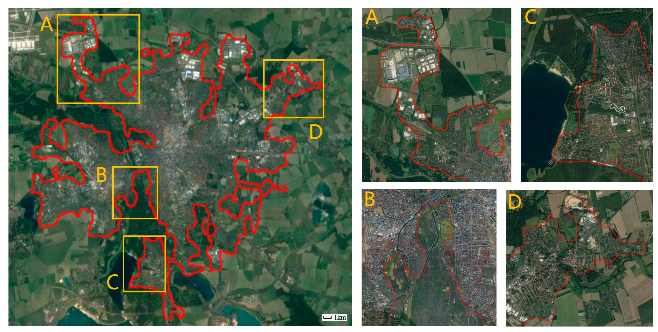
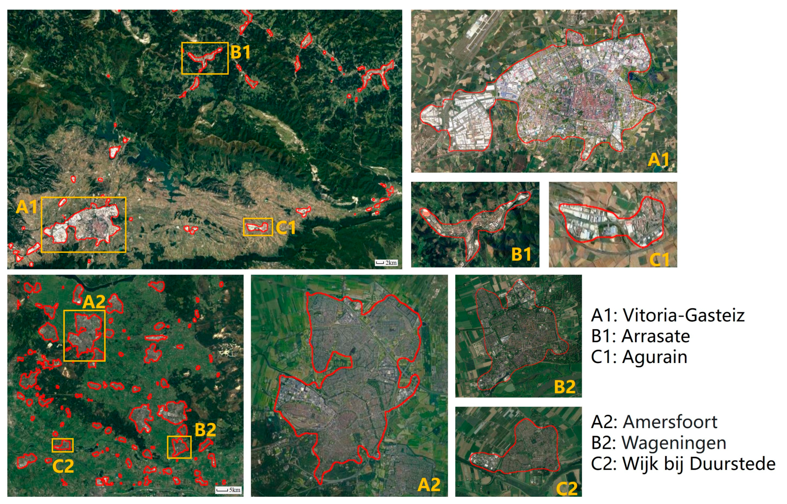
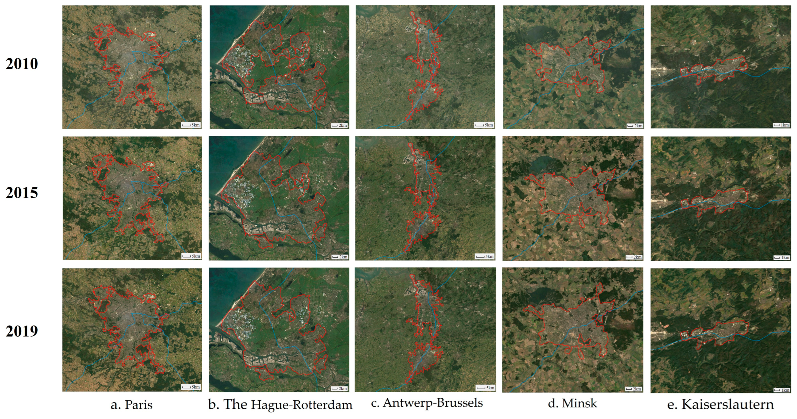
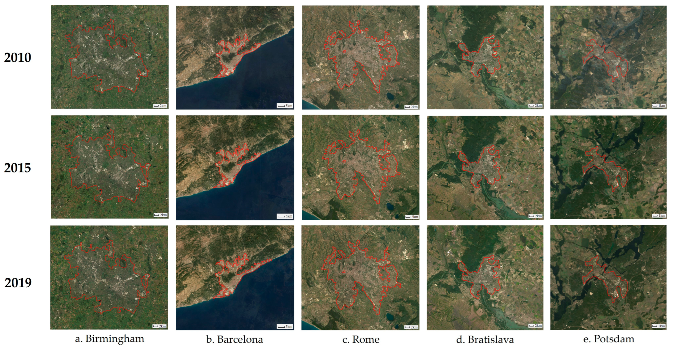
3.1.1. Comparison with Historical Google Imagery

The proposed mapping approach is capable of capturing the dynamics of urban expansion robustly both in large and regional urban clusters. We first selected the urban cluster of Leipzig, Germany, in 2019 for comparison with the urban dynamics derived from Landsat (Figure 4). Germany was one of the first countries to establish the CRE and Leipzig is a representative of the ”online” city. According to the overall result and four local enlargements, the EUB can capture dynamic changes within the urban area in fine detail. The city boundary delineated by the EUB includes most impermeable areas but excludes small urban patches around the edge of the city boundary (as shown in Figure 4A). This indicates that the proposed urban boundary delineation method is well suited for medium-resolution and high-resolution urban areas with relatively high heterogeneity within cities.

Figure 5 shows the spatial distributions of the time-series EUB for this city from 2000–2019 with intervals of 5 years. Although it has been reported that the impervious area expansion ratios of European countries were slow, there is a notable expansion of urban areas in Leipzig after 2010. The urban boundary dynamics from the GISA2 data clearly capture this urban expansion with almost identical boundaries captured by the Landsat result.

Urban regions can exhibit a range of spatial configurations, from densely aggregated to broadly dispersed urban sprawls. This variation in the urban footprint poses a significant challenge to the process of extracting the EUB, impacting both the spatial resolution required and the precision of delineation. To rigorously evaluate the efficacy of the EUB extraction methodology across different urban morphologies, we have strategically chosen specific cities as case studies. Vitoria-Gasteiz in Spain and Amersfoort in the Netherlands serve as examples of highly integrated, contiguous urban environments, typifying aggregated city structures. In contrast, Arrasate and Agurain in Spain, along with Wageningen and Wijk bij Duurstede in the Netherlands, have been selected for their dispersed urban patterns, which exemplify scattered city formations. These cities were chosen based on their distinctive spatial characteristics, which are representative of the broader category they belong to, and will enable a comprehensive assessment of the EUB extraction technique’s versatility and accuracy. As shown in Figure 6, aggregated and scattered cities can both be effectively identified, since the spatial connectivity between urban areas and their surrounding regions has been fully considered in our workflow. More specifically, aggregated cities consisting of closely connected small clusters are defined as a large metropolitan area (zooming in as Figure 6A1, A2). Isolated scattered cities are designated as independent urban areas (zooming in as Figure 6B1, B2, C1, C2). Though these scattered cities are small, a good consistency can be observed between the extracted EUB with the urban extent in the high-resolution Google Earth imagery.

When extending our workflow to other cities in our study area entirely, the produced EUB results can effectively capture the spatial extent of their urban areas. In total, 1.65 million km² of urban areas in 2019 have been mapped, and a good match can be visually observed in Figure 7 by overlaying the generated EUB for six representative ON-CRE cities, i.e., Hannover (Germany), Warszawa (Poland), Prague (Czech), Madrid (Spain), Budapest (Hungary), and Marseille (France), on Google Earth imageries. Although the spatial patterns of these cities are diverse, for example, Madrid and Budapest have different branches in their urban edge regions, making it rather difficult to precisely capture the tiny urban branches as well as the urban main body simultaneously, it can be observed that the boundaries can clearly distinguish between urban and non-urban areas surrounding cities due to the multiscale strategy in the proposed framework.

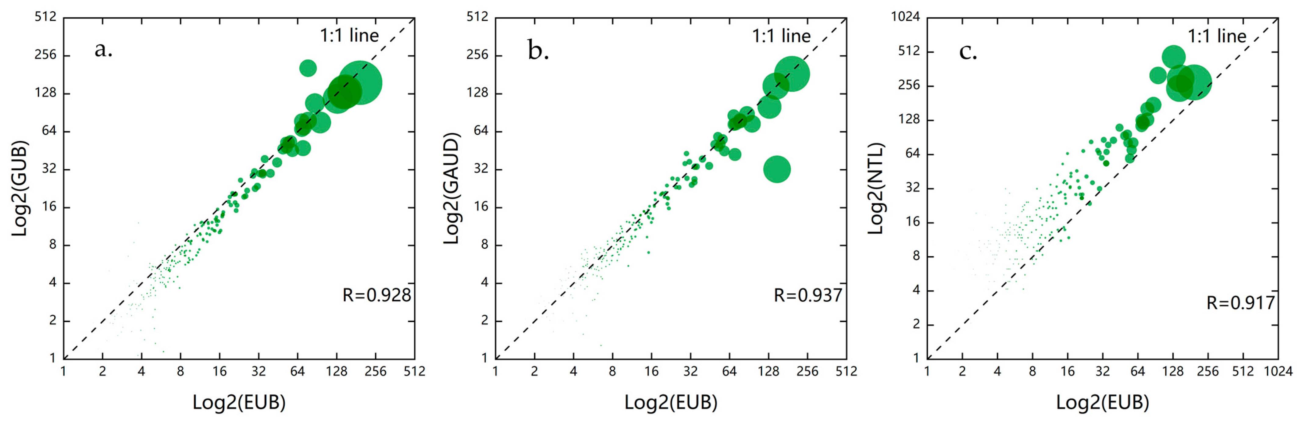
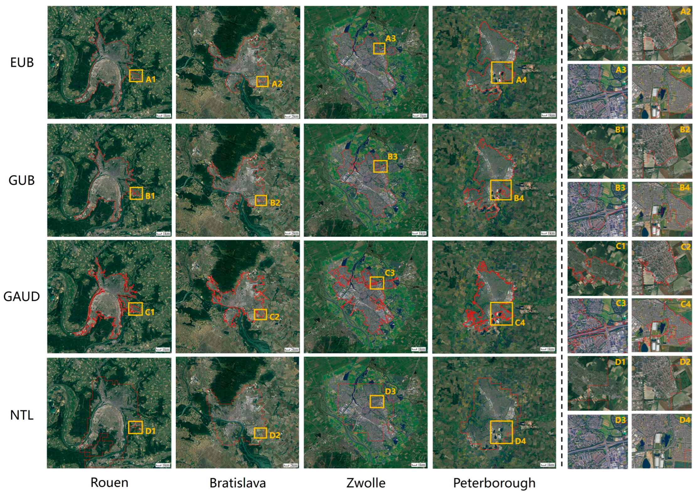
3.1.2. Cross-Comparisons with Other Global 30 m Urban Products

With the development in computing and storage capabilities, global urban boundary mapping has become achievable, such as the GUB generated by Li [32] et al. with a spatial resolution of 30 m, the GAUD where urban dynamics were extracted using temporal segmentation from the annual Normalized Urban Area Convergence Index (NUACI), and the NTL based on the area exhibiting the most significant change in NTL luminance along the urban–rural gradient, following the approach outlined by Zhou [44]. To assess the consistency of the EUB results with previous impervious surface products, the scatterplots and the corresponding regression functions are illustrated in Figure 8. It should be noted that the detailed global ISA expansion analysis is beyond the scope of this study, and here we only made a preliminary comparison between urban sizes derived from each dataset in the scatter points.

As shown in Figure 8, from observing the long time-series dynamics, the consistency between the EUB and other products increased, and the regression slope also increasingly approached 1.0, with correlation coefficients (R values) being 0.928 (with GUB), 0.937 (with GAUD), and 0.917 (with NTL). Specifically, as for the scatterplots between the GUB and EUB, most scatter points were obviously concentrated below the 1:1 line at the early stage, and slowly turned to distribute on both sides of the 1:1 line (Figure 8a). On the other hand, as the NTL-based urban boundary primarily relies on the emitted lights from cities during nighttime, inadvertently encompassing urban-related elements such as lakes and parks [22], we could find that most scatter points were located above the 1:1 line, and the regression slopes were larger than 1.0 (Figure 8c). Comparatively, there was greater agreement between the GAUD and EUB than between other products in terms of the spatial distributions of the scatter points and the regression slope (Figure 8b).

To intuitively compare the produced urban boundaries from these four impervious products, four validation regions with various impervious landscapes from different parts of the European continent, including Rouen (France), Bratislava (Slovakia), Zwolle (Netherland), and Peterborough (United Kingdom), were selected for presentation in Figure 9. Despite the relatively good agreement between the four urban boundary results at different city scales, differences can be inferred from the enlarged results marked with A1-D4: (1) Benefiting from the high consistency of GISA2 and multiscale morphological processing, the EUB results accurately capturing the central and peripheral impervious objects had significant agreement with the base Landsat maps; (2) the GUB performed well in most of the urban regions, but underestimated some peripheral urban areas (B1 and B3). This omission error possibly came from the sparse training samples in GAIA producing; (3) the GAUD accurately delineated the central and peripheral impervious objects (C2), but excluded rural areas and other pervious objects (e.g., lakes and grassland) in the urban regions (C3 and C4), which was partly responsible for the underestimation of urban sizes; (4) the NTL had the biggest impervious areas among several products, but it misclassified the vegetation and bare soils into impervious surfaces, resulting in overestimation (D1–D4).

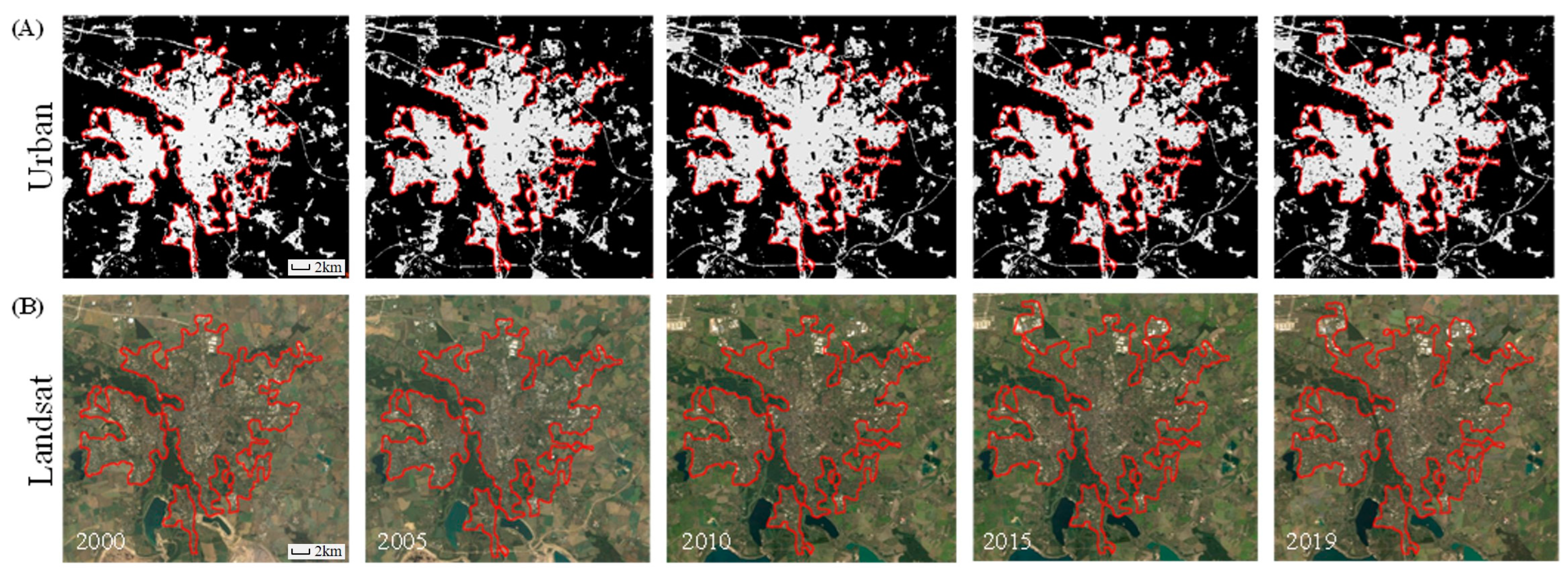
3.2. The Spatiotemporal Dynamics of Urban Boundaies from 2010 to 2019

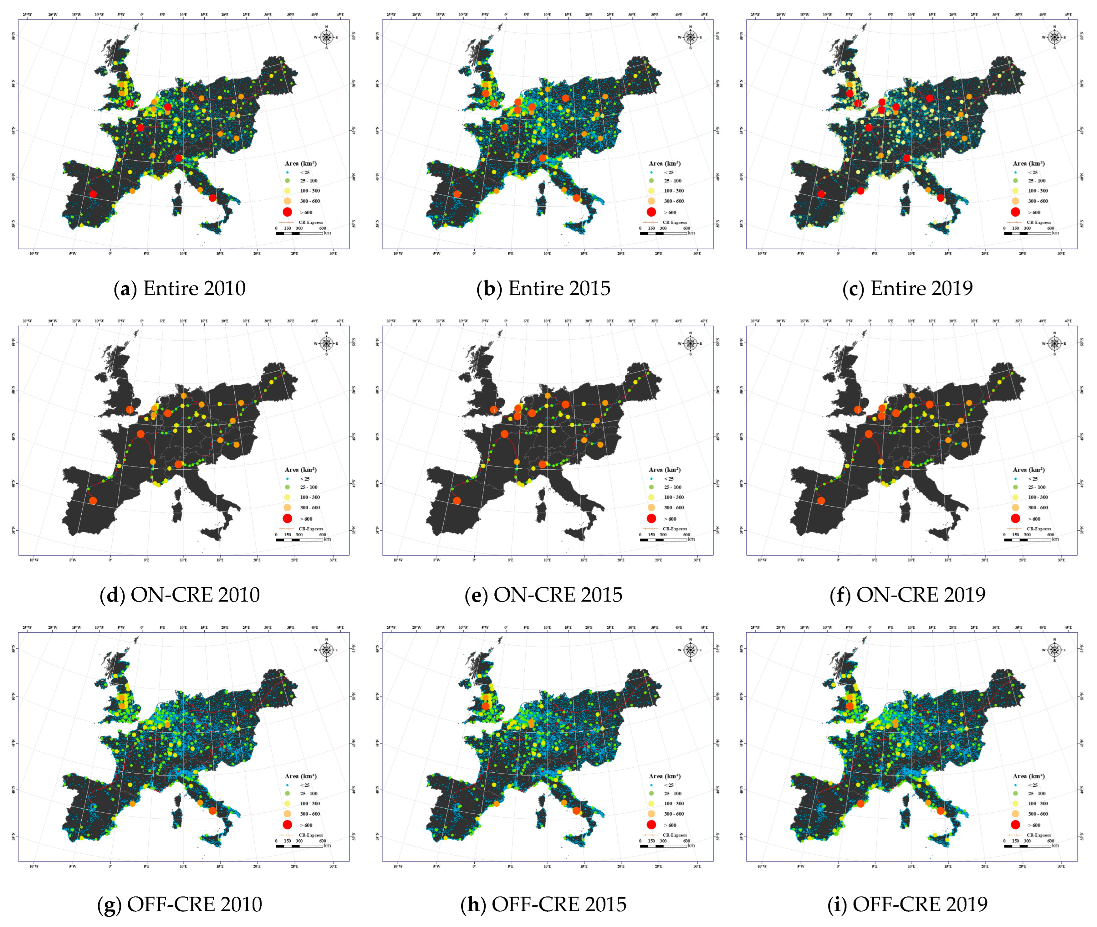
3.2.1. Spatiotemporal Patterns Urban Clusters

To analyze the urban expansion patterns of different countries, we calculated the areas of urban clusters based on the annual EUB results during different phases of the CRE establishment, aligning with the construction phase (2010–2013), initial operation phase (2013–2015), and stable operation phase (2015–2019). Figure 10a–i delineate the spatial distribution of urban clusters (greater than 25, 100, 300, and 600 km²) for the years 2010, 2015, and 2019. Each size category is characterized by unique hues and denoted as L1–L5 tiers. On a continent scale, numerous cities exhibit expansion trends, while others remain stable or experience a decline. Furthermore, considerable disparities in the urban extents could be observed between cities situated within and outside the CRE corridor (designated as ON-CRE and OFF-CRE, respectively).

We subsequently aggregated the total counts of cities falling into the five tiers over the period from 2010 to 2019 and reported their fluctuations in

Table 2. Dynamics of urban area and cluster numbers for L1–L5 tiers from 2000 to 2019.

Entire Study Area
Area (number)	L1	L2	L3	L4	L5	Total
2010	25,513.4 (3547)	14,969.0 (334)	8300.4 (50)	6186.2 (14)	6650.3 (6)	61,619.4 (3951)
2015	26,258.2 (3620)	15,157.4 (331)	8497.6 (51)	4566.8 (11)	9333.3 (10)	63,813.4 (4023)
2019	28,811.8 (3973)	17,284.5 (376)	10,386.1(63)	4184.4 (10)	10,287.6 (11)	70,954.4 (4433)
ON-CRE
Area (number)	L1	L2	L3	L4	L5	Total
2010	1791.3 (218)	1956.2 (42)	3437.8 (18)	3650.1 (9)	5699.1 (5)	16,534.5 (292)
2015	1874.8 (225)	1971.4 (42)	3478.2 (18)	2278.9 (6)	7745.9 (8)	17,349.2 (299)
2019	1998.5 (233)	2319.7 (47)	3754.6 (18)	2359.0 (6)	7956.2 (8)	18,387.9 (312)
OFF-CRE
Area (number)	L1	L2	L3	L4	L5	Total
2010	23,722.1 (3329)	13,012.9 (292)	4862.5 (32)	2536.1 (5)	951.2 (1)	45,084.8 (3659)
2015	24,383.4 (3395)	13,186.0 (289)	5019.4 (33)	2288.0 (5)	1587.4 (2)	46,464.2 (3724)
2019	27,026.5 (3769)	14,962.8 (329)	6627.6 (45)	1797.6 (4)	2331.4 (3)	52,746.0 (4150)

Note: the shades of blue represent the highest values of urban area and cluster numbers.

. As shown in Figure 10, the cumulated urban areas for 2010, 2015, and 2019 amount to 61,619.4 km², 63,813.4 km², and 70,954.4 km², with the number of clusters totaling 3951, 4023, and 4433, indicating a comprehensive expansion throughout the entire region. When examining the evolution within distinct tiers, we observed an increase of 3637.3 km² and 954.2 km² of L5-tier cities (greater than 600 km²) for the year 2019, compared to 2010 and 2015. When checking Figure 11a–c, the quantity of L5-tier clusters increased from 6 (in 2010) to 10 (in 2015) and 11 (in 2019), respectively. Berlin (ON-CRE), Den Haag–Rotterdam (ON-CRE), Antwerpen–Brussel (ON-CRE), Birmingham (OFF-CRE), and Barcelona (OFF-CRE) were newly included in this tier. These expansions contribute to a reduction in both the area and clusters for the L4 tier (greater 300 km²): the area decreased from 6186.2 km² to 4566.8 km² in 2015 and further to 4184.5 km² in 2019, compared with 2010; the number of clusters decreased from 14 to 11 in 2015 and to 10 in 2019.

Figure 11 quantitatively summarizes the dynamics of proportions for the L1–L5-tiered urban clusters pertaining to ON-CRE, OFF-CRE, and the entire study area. Evidently, the proportion of L5-tier clusters in ON-CRE regions experienced the most significant increase, from 34.5% in 2010 to 43.3% in 2019, while the proportion in L4-tier clusters markedly decreased from 22.1% to 12.8%, and the L1 to L3 tiers exhibited a slight increase. Given that the total urban area also expanded as the time progressed, from 16,534.5 km² to 18,387.9 km² for ON-CRE, this is likely attributed to two sources: (1) the transformation from rural settlements to urban built-up, and (2) the establishment of new towns and urban organic decentralization. In contrast, their area expansion ratios were relatively low for OFF-CRE regions, and the proportions for L1–L5 tiers remained stable, as the urbanization level in most European countries was consistently high for the past three decades [23].

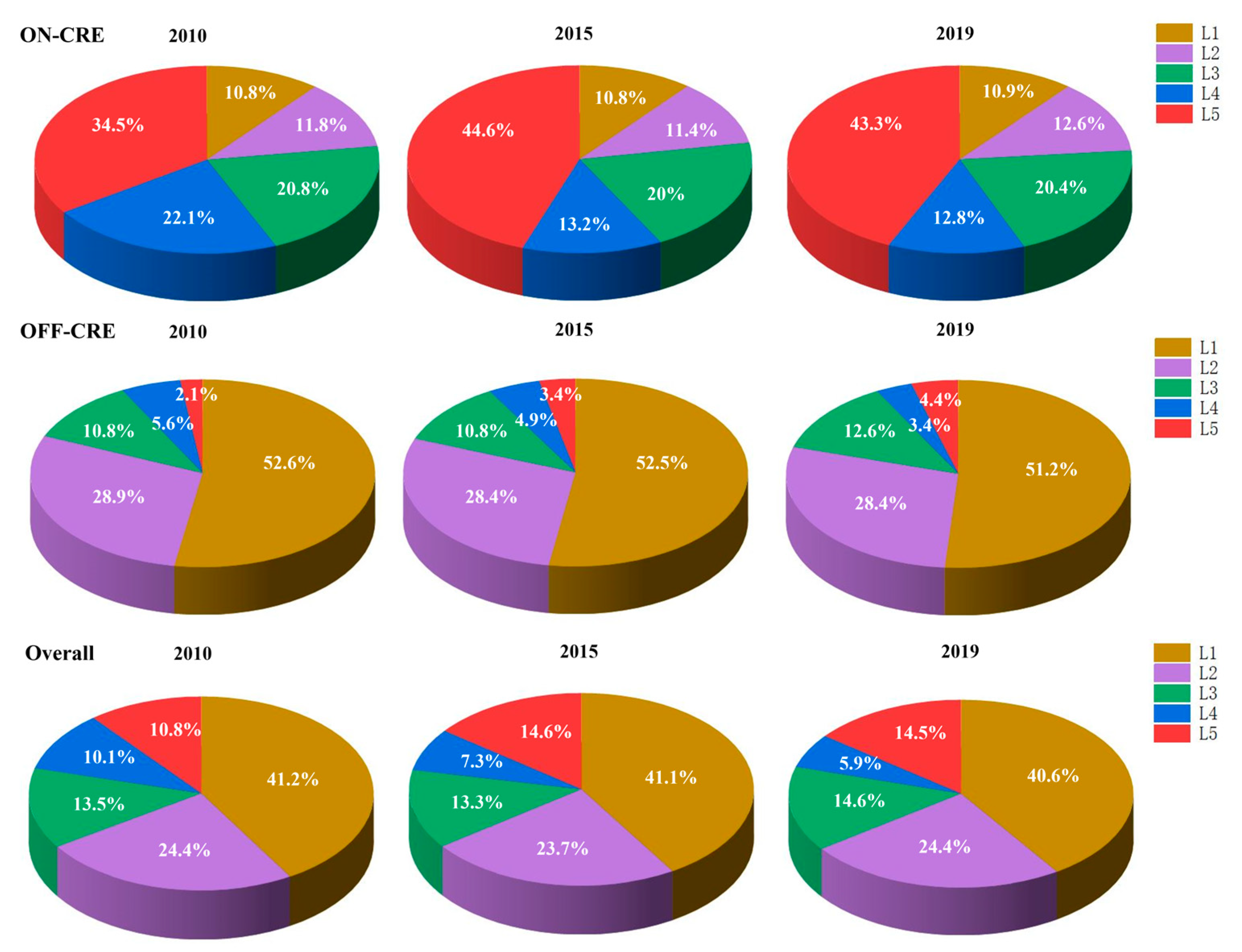
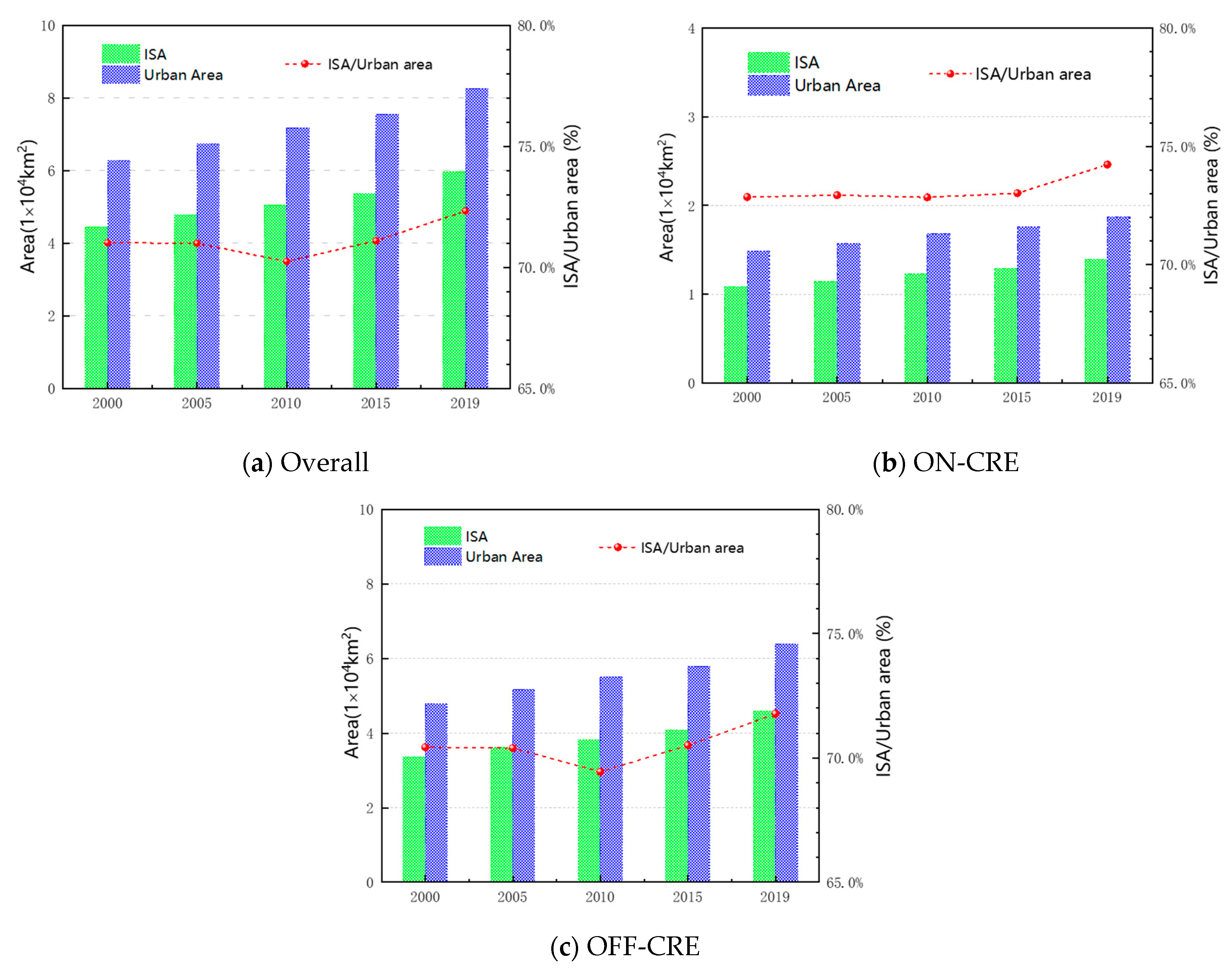
3.2.2. Comparison of Spatial Dynamics between ON-CRE and OFF-CRE Cities

Ten cities were selected to compare the spatial dynamics of ON-CRE and OFF-CRE cities by considering the city size, spatial distribution, and urban landscapes. Among them, the five ON-CRE cities were Paris (France, L5), the Hague–Amsterdam (Netherlands, L4–L5), Antwerp–Brussels (Belgium, L4–L5), Minsk (Belarus, L3–L4), and Kaiserslautern (L1–L2). Their urban boundaries in 2010, 2015, and 2019 are presented in Figure 12 with red solid lines, while the blue dashed lines represent the CRE locations.

From visual interpretation, large cities (Figure 12a) are less influenced in terms of urban morphology due to their highly developed urban conditions. The expansion results (

Table 3. The population, area, and expansion rate of five ON-CRE cities.

	Paris	The Hague–Rotterdam	Antwerp– Brussels	Minsk	Kaiserslautern
Population (m)	2.2	1.7	2.8	2.0	0.1
Area (2010, km2)	1474.63	498.65	660.11	230.16	24.63
Area (2015, km2)	1501.6	624.95	683.85	253.98	26.11
Area (2019, km2)	1540.27	647.269	711.5	274.18	27.04
Expansion rates (2010–2015)	1.83%	25.33%	3.60%	10.35%	6.03%
Expansion rates (2015–2019)	2.58%	3.57%	4.04%	7.95%	3.57%

Note: The population data in Table 3 and Table 4 are sourced from World Population Review (https://worldpopulationreview.com accessed on 2 February 2024) in 2020. Population unit is in millions. Area data are sourced from the city boundary data we generated, with the unit in km².

) show that Paris’s expansion rate is 1.83% (2010–2015) and 2.58% (2015–2019). Newly included in L5, the agglomerations of Hague–Rotterdam (Figure 12b) and Antwerp–Brussels (Figure 12c) are noteworthy, as frequent interactions between cities have spurred the urbanization process along the express, thus connecting cities to form urban agglomerations. Minsk has not undergone significant changes visually, but urban expansion can be observed occurring in the northern and southern areas traversed by the express, with an overall expansion rate of 10.35% (2010–2015) and 7.95% (2015–2019). Kaiserslautern represents the developing pattern of emerging cities, which have achieved rapid progress in the urban extents and expansion rates (6.03%, 2010–2015 and 3.75%, 2015–2019) during the past decade. Although the number of urban clusters has not grown significantly for L1–L3 tiers, this may be due to the decrease in the number of urban clusters resulting from the merging of surrounding small cities. Additionally, comparing the locations of the CRE and city expansion trajectories, more changes occurred along the express than in non-aligned areas. This may be attributed to the operation of the express and the turnover of freights, which bring new job opportunities and attract the construction of supporting infrastructures.

The five selected OFF-CRE cities were Birmingham (UK, L4–L5), Barcelona (Spain, L4–L5), Rome (Italy, L4), Bratislava (L2–L3), and Potsdam (L1–L2). Their spatial dynamics, presented in Figure 13, align well with the overall dynamics in terms of the area and quantity reported in Table 2, demonstrating stable development with no significant changes in urban boundaries. In contrast to most OFF-CRE cities, Birmingham and Barcelona have experienced extensive expansion, while the other three cities exhibit expansion rates around 2% (

Table 4. The population, area, and expansion rate of five OFF-CRE cities.

	Birmingham	Barcelona	Rome	Bratislava	Potsdam
Population (m)	2.6	5.5	4.2	0.4	0.2
Area (2010, km2)	593.51	576.64	383.07	98.02	24.46
Area (2015, km2)	603.53	586.47	395.04	99.87	25.53
Area (2019, km2)	607.22	649.74	404.43	101.85	26.93
Expansion rates (2010–2015)	1.69%	1.71%	3.12%	1.89%	4.36%
Expansion rates (2015–2019)	0.61%	3.57%	2.38%	1.98%	5.48%

).

As the proposed EUB is defined to be larger than the impervious surface area (ISA), we created a bar chart (Figure 14) to compare the ISA and EUB for the period of 2000–2019 with a 5-year interval. It is obvious that a positive correlation exists between the two areas on a general level. The total urban area (urban clusters greater than 1 km²) measured 62,660 km², 67,248 km², 71,801 km², 75,480 km², and 82,536 km², and the proportion of the ISA within urban areas varied. In order to comprehend this variation, we calculated the ISA ratio and presented it with the dot lines. Specifically, 71.01% of the delineated EUB was comprised of impervious areas in 2000, with impervious areas making up about 70.24% and 72.32% of this area in 2010 and 2019. It should be noted that the EUB results only encompass impervious areas within the designated limits and do not include small or dispersed urban areas beyond these boundaries. It can be found that there is a slight drop in 2010, which should be owed to the relative lower speed in urban sprawl.

Urban growth shows different patterns and pathways for ON and OFF CRE cities, and it appears that ON-CRE cities experienced a more pronounced expansion of urban areas from 2010 to 2019. The changing characteristics of OFF-CRE cities that are demonstrated are similar with those of overall cities when comparing Figure 14a,c. There is a general increasing trend in both the urban areas and ISA from 2000–2019 for the ON-CRE cities but it shows rather different changing rates and turning points according to Figure 13b. The total urban area (urban clusters greater than 1 km²) measured about 14,890 km² in 2000. This number increased by 12.89% (16,810 km²) in 2010, and 25.49% (18,686 km²) in 2019. In this region, the proportion of the ISA within the EUB stands at approximately 72%. It subtly declined from 2000 to 2010, followed by a consistently increasing trend from 2010 to 2019. The growth rate shifted from 0.18% (2010–2015) to 1.26% (2015–2019), culminating in an ISA proportion of 74.2%, indicating more compact impervious areas within the boundaries in this part than OFF-CRE regions. This is likely attributed to the notable urban expansion over the past few decades, coupled with the influence of the inauguration of the CRE.

4. Discussion

In this study, we employed the GISA2 dataset on the GEE platform to refine urban boundaries, resulting in the EUB dataset. The results presented in this study demonstrate the effectiveness and applicability of the EUB approach in capturing the spatiotemporal dynamics of urban expansion across Europe, particularly in areas within and outside the CRE corridor. Here, we discuss the key findings and their implications in detail.

The comparison of the EUB results with historical Google imagery showcases the robustness of our mapping approach in capturing the urban expansion dynamics, even in regions characterized by high urban heterogeneity. The precise delineation of urban boundaries in cities like Leipzig, Germany, demonstrates the method’s adaptability to urban environments of varying resolutions. When comparing the EUB outputs with established global urban datasets like the GUB, GAUD, and NTL, we observe a slight overestimation of smaller urban extents in the EUB compared to the GUB, while maintaining consistency with the GAUD measurements. For cities exceeding a certain size, our results align well with the urban sizes obtained from the GUB, albeit slightly larger than those from the GAUD. This divergence can be attributed to variances in the definitions and methodologies employed for delineating urban boundaries in these two reference datasets.

Our analysis discerns heterogeneous urban growth patterns within the different phases of CRE development. Cities along the CRE corridor showcase distinct expansion trends compared to those outside it, highlighting the corridor’s substantial influence on urban proliferation. Notably, the rise of megacities and emergence of new urban clusters reflect the complex dynamics of urbanization within the study area. The formation of these megacities (L4–L5 tiers) is likely associated with the expansion of cities and their merging with neighboring small cities. Although such a merging process will reduce the number of urban clusters, the total number of urban clusters in more than 90% of countries has been increasing over the past few decades due to the growth of massive small urban clusters, similar to Zhang’s study [45]. Additionally, a general increase in diminutive and moderate cities (L1–L3 tiers) can be observed, suggesting that more urban clusters have emerged with local development. Resonating with observations by Dong [46], we found the overall expansion of cities in the European region is not significant. However, a comparison between the ON-CRE and OFF-CRE cities still highlights different expansion trajectories, with ON-CRE cities experiencing more significant urban growth, consistent with insights from Zhang [47]. This is attributed to factors like infrastructural enhancements and transportation planning, which facilitate the transformation of urban agglomerations into urban clusters. In contrast, the expansion of cities in the OFF-CRE region is relatively limited. The restricted urban sprawl is primarily attributed to their moderate sizes and compact patterns, as well as general infrastructure development, consistent with the findings by Nickayin [48]. Historical factors, such as the city–state tradition, have fostered balanced growth between historical and emerging urban areas. Another contributing factor is the high level of development commonly found in Europe, which further stabilizes urban growth and restrains excessive expansion, with expansion exhibiting a trend towards central compactness [46]. In contrast to most OFF-CRE cities, we found that cities near or along the coast have experienced extensive expansion, which is mainly attributed to accelerated development policies in coastal areas, aligning with findings from other studies [49,50,51].

This study also has certain limitations. It relies on the GISA2 dataset (1972–2019), and while the classification accuracy of these data may impact the precision of our quantitative assessments, we are unable to refresh our analysis with data post-2020. Identifying urban boundaries in regions with complex spatial patterns remains a challenge, requiring further algorithm improvements and the integration of multiple data sources. Moreover, disparities in the CRE establishment time, operational intensities, and regional and national policy may influence variations in urban sizes.

5. Conclusions

Based on the global impervious surface area (GISA2) product, this study developed an EUB extraction process on the Google Earth Engine platform to generate annual European urban boundary products from 2010 to 2019. The EUB method employs a multiscale combination of kernel density estimation and morphological techniques. In comparison with the Landsat time-series data, the EUB accurately delineates city boundaries of various sizes and shapes, exhibiting consistency with existing fine-resolution (30 m) products.

Throughout the study period, urban areas and clusters expanded across the entire region, with notable disparities observed between ON-CRE and OFF-CRE cities. ON-CRE cities exhibited more substantial urban growth. Although megacities experienced minimal influence on urban morphology due to their highly developed conditions, new mega urban agglomerations (e.g., Hague–Amsterdam and Antwerp–Brussels) emerged along the expressway, resulting from frequent city interactions. Meanwhile, small and moderate (L1 and L2 tiers) cities showed a general increase, indicating the emergence of more urban clusters through local development. Among the OFF-CRE cities, Birmingham and Barcelona underwent extensive expansion due to accelerated coastal development policies, while other OFF-CRE cities displayed stable development with limited urban sprawl, attributable to their moderate sizes, compact patterns, and advanced development levels. Moreover, the proportion of the impervious surface area (ISA) within the EUB slightly decreased from 2000 to 2010 but consistently rose from 2010 to 2019, signifying more compact impervious areas within ON-CRE boundaries compared to those in OFF-CRE.

This study offers a fine-scaled annual city boundaries and expansions dataset for the CRE area, contributing to the understanding of urban expansion driven by the long-term operation of the CRE over the past decade and supporting the promotion of sustainable urban development. Given the varying times of CRE establishment and different operational intensities, as well as the diverse ecological, economic, and policy conditions across different countries and regions, our future research will focus on specific countries and cities. We aim to conduct fine-grained assessments, comprehensively analyze various influencing factors, and determine the net impact of the CRE on urban expansion.

References

1. Gong, J.; Liu, C.; Huang, X. Advances in urban information extraction from high-resolution remote sensing imagery. Sci. China Earth Sci. 2020, 63, 463–475. [Google Scholar] [CrossRef]
2. Liu, Y.; Ou, C.; Li, Y.; Zhang, L.; He, J. Regularity of rural settlement changes driven by rapid urbanization in North China over the three decades. Sci. Bull. 2023, 68, 2115–2124. [Google Scholar] [CrossRef]
3. Song, Y.; Chen, B.; Kwan, M.-P. How does urban expansion impact people’s exposure to green environments? A comparative study of 290 Chinese cities. J. Clean. Prod. 2020, 246, 119018. [Google Scholar] [CrossRef]
4. Hafeez, M.; Yuan, C.; Shah, W.U.H.; Mahmood, M.T.; Li, X.; Iqbal, K. Evaluating the relationship among agriculture, energy demand, finance and environmental degradation in one belt and one road economies. Carbon Manag. 2020, 11, 139–154. [Google Scholar] [CrossRef]
5. Liu, H.; Gu, W.; Liu, W.; Wang, J. The influence of China-Europe Railway Express on the production system of enterprises: A case study of TCL Poland Plant. J. Geogr. Sci. 2021, 31, 699–711. [Google Scholar] [CrossRef]
6. Wu, Q.; Madni, G.R. Environmental protection in selected one belt one road economies through institutional quality: Prospering transportation and industrialization. PLoS ONE 2021, 16, e0240851. [Google Scholar] [CrossRef] [PubMed]
7. Zhai, W. Risk assessment of China’s foreign direct investment in “One Belt, One Road”: Taking the green finance as a research perspective. Socio-Econ. Plan. Sci. 2023, 87, 101558. [Google Scholar] [CrossRef]
8. Zhao, M.; Zhou, Y.; Li, X.; Cheng, W.; Zhou, C.; Ma, T.; Li, M.; Huang, K. Mapping urban dynamics (1992–2018) in Southeast Asia using consistent nighttime light data from DMSP and VIIRS. Remote Sens. Environ. 2020, 248, 111980. [Google Scholar] [CrossRef]
9. Shao, Z.; Liu, C. The Integrated Use of DMSP-OLS Nighttime Light and MODIS Data for Monitoring Large-Scale Impervious Surface Dynamics: A Case Study in the Yangtze River Delta. Remote Sens. 2014, 6, 9359–9378. [Google Scholar] [CrossRef]
10. Chen, Z.; Yu, B.; Song, W.; Liu, H.; Wu, Q.; Shi, K.; Wu, J. A New Approach for Detecting Urban Centers and Their Spatial Structure With Nighttime Light Remote Sensing. IEEE Trans. Geosci. Remote Sens. 2017, 55, 6305–6319. [Google Scholar] [CrossRef]
11. Zhuo, L.; Zheng, J.; Zhang, X.; Li, J.; Liu, L. An improved method of night-time light saturation reduction based on EVI. Int. J. Remote Sens. 2015, 36, 4114–4130. [Google Scholar] [CrossRef]
12. Arnold, C.L., Jr.; Gibbons, C.J. Impervious Surface Coverage: The Emergence of a Key Environmental Indicator. J. Am. Plan. Assoc. 1996, 62, 243–258. [Google Scholar] [CrossRef]
13. Gutiérrez-Rial, D.; Soto González, B.; García Vázquez, D.; Méndez-Martínez, G.; Pombal Diego, M.Á.; Garrido González, J. Freshwater biodiversity loss in urbanised rivers. Ecol. Indic. 2023, 156, 111150. [Google Scholar] [CrossRef]
14. Hanh Nguyen, H.; Venohr, M.; Gericke, A.; Sundermann, A.; Welti, E.A.R.; Haase, P. Dynamics in impervious urban and non-urban areas and their effects on run-off, nutrient emissions, and macroinvertebrate communities. Landsc. Urban Plan. 2023, 231, 104639. [Google Scholar] [CrossRef]
15. Oswald, C.J.; Kelleher, C.; Ledford, S.H.; Hopkins, K.G.; Sytsma, A.; Tetzlaff, D.; Toran, L.; Voter, C. Integrating urban water fluxes and moving beyond impervious surface cover: A review. J. Hydrol. 2023, 618, 129188. [Google Scholar] [CrossRef]
16. García, D.H.; Díaz, J.A. Space–time analysis of the earth’s surface temperature, surface urban heat island and urban hotspot: Relationships with variation of the thermal field in Andalusia (Spain). Urban Ecosyst. 2023, 26, 525–546. [Google Scholar] [CrossRef]
17. Li, L.; Zhan, W.; Hu, L.; Chakraborty, T.C.; Wang, Z.; Fu, P.; Wang, D.; Liao, W.; Huang, F.; Fu, H.; et al. Divergent urbanization-induced impacts on global surface urban heat island trends since 1980s. Remote Sens. Environ. 2023, 295, 113650. [Google Scholar] [CrossRef]
18. Li, C.; Yang, J.; Zhang, Y. Evaluation and Analysis of the Impact of Coastal Urban Impervious Surfaces on Ecological Environments. IEEE J. Sel. Top. Appl. Earth Obs. Remote Sens. 2023, 16, 8721–8733. [Google Scholar] [CrossRef]
19. Wang, Y.; Li, M. Urban Impervious Surface Detection from Remote Sensing Images: A review of the methods and challenges. IEEE Geosci. Remote Sens. Mag. 2019, 7, 64–93. [Google Scholar] [CrossRef]
20. Xie, Y.; Weng, Q. Spatiotemporally enhancing time-series DMSP/OLS nighttime light imagery for assessing large-scale urban dynamics. ISPRS J. Photogramm. Remote Sens. 2017, 128, 1–15. [Google Scholar] [CrossRef]
21. Gong, P.; Li, X.; Wang, J.; Bai, Y.; Chen, B.; Hu, T.; Liu, X.; Xu, B.; Yang, J.; Zhang, W.; et al. Annual maps of global artificial impervious area (GAIA) between 1985 and 2018. Remote Sens. Environ. 2020, 236, 111510. [Google Scholar] [CrossRef]
22. Liu, X.; Huang, Y.; Xu, X.; Li, X.; Li, X.; Ciais, P.; Lin, P.; Gong, K.; Ziegler, A.D.; Chen, A.; et al. High-spatiotemporal-resolution mapping of global urban change from 1985 to 2015. Nat. Sustain. 2020, 3, 564–570. [Google Scholar] [CrossRef]
23. Huang, X.; Li, J.; Yang, J.; Zhang, Z.; Li, D.; Liu, X. 30 m global impervious surface area dynamics and urban expansion pattern observed by Landsat satellites: From 1972 to 2019. Sci. China Earth Sci. 2021, 64, 1922–1933. [Google Scholar] [CrossRef]
24. Melchiorri, M.; Florczyk, A.J.; Freire, S.; Schiavina, M.; Pesaresi, M.; Kemper, T. Unveiling 25 Years of Planetary Urbanization with Remote Sensing: Perspectives from the Global Human Settlement Layer. Remote Sens. 2018, 10, 768. [Google Scholar] [CrossRef]
25. Shao, Z.; Cheng, T.; Fu, H.; Li, D.; Huang, X. Emerging Issues in Mapping Urban Impervious Surfaces Using High-Resolution Remote Sensing Images. Remote Sens. 2023, 15, 2562. [Google Scholar] [CrossRef]
26. Melchiorri, M.; Pesaresi, M.; Florczyk, A.J.; Corbane, C.; Kemper, T. Principles and Applications of the Global Human Settlement Layer as Baseline for the Land Use Efficiency Indicator—SDG 11.3.1. ISPRS Int. J. Geo-Inf. 2019, 8, 96. [Google Scholar] [CrossRef]
27. Huang, X.; Song, Y.; Yang, J.; Wang, W.; Ren, H.; Dong, M.; Feng, Y.; Yin, H.; Li, J. Toward accurate mapping of 30-m time-series global impervious surface area (GISA). Int. J. Appl. Earth Obs. Geoinf. 2022, 109, 102787. [Google Scholar] [CrossRef]
28. Ren, H.; Liu, Y.; Chang, X.; Yang, J.; Xiao, X.; Huang, X. Mapping High-Resolution Global Impervious Surface Area: Status and Trends. IEEE J. Sel. Top. Appl. Earth Obs. Remote Sens. 2022, 15, 7288–7307. [Google Scholar] [CrossRef]
29. Liang, X.; Guan, Q.; Clarke, K.C.; Liu, S.; Wang, B.; Yao, Y. Understanding the drivers of sustainable land expansion using a patch-generating land use simulation (PLUS) model: A case study in Wuhan, China. Comput. Environ. Urban Syst. 2021, 85, 101569. [Google Scholar] [CrossRef]
30. Sun, Z.; Du, W.; Jiang, H.; Weng, Q.; Guo, H.; Han, Y.; Xing, Q.; Ma, Y. Global 10-m impervious surface area mapping: A big earth data based extraction and updating approach. Int. J. Appl. Earth Obs. Geoinf. 2022, 109, 102800. [Google Scholar] [CrossRef]
31. Wang, Y.; Ziv, G.; Adami, M.; Mitchard, E.; Batterman, S.A.; Buermann, W.; Schwantes Marimon, B.; Marimon Junior, B.H.; Matias Reis, S.; Rodrigues, D.; et al. Mapping tropical disturbed forests using multi-decadal 30 m optical satellite imagery. Remote Sens. Environ. 2019, 221, 474–488. [Google Scholar] [CrossRef]
32. Li, X.; Gong, P.; Zhou, Y.; Wang, J.; Bai, Y.; Chen, B.; Hu, T.; Xiao, Y.; Xu, B.; Yang, J.; et al. Mapping global urban boundaries from the global artificial impervious area (GAIA) data. Environ. Res. Lett. 2020, 15, 094044. [Google Scholar] [CrossRef]
33. Worldmeter. Available online: https://www.worldometers.info/population/countries-in-europe-by-population/ (accessed on 16 July 2023).
34. Althouse, J.; Cahen-Fourot, L.; Carballa-Smichowski, B.; Durand, C.; Knauss, S. Ecologically unequal exchange and uneven development patterns along global value chains. World Dev. 2023, 170, 106308. [Google Scholar] [CrossRef]
35. Heiskanen, E.; Matschoss, K. Understanding the uneven diffusion of building-scale renewable energy systems: A review of household, local and country level factors in diverse European countries. Renew. Sustain. Energy Rev. 2017, 75, 580–591. [Google Scholar] [CrossRef]
36. National Development and Reform Commission (NDRC) People’s Republic of China. Available online: https://www.ndrc.gov.cn/xwdt/xwfb/202208/t20220818_1333176.html (accessed on 18 August 2022).
37. Gong, P.; Liu, H.; Zhang, M.; Li, C.; Wang, J.; Huang, H.; Clinton, N.E.; Ji, L.; Li, W.; Bai, Y.; et al. Stable classification with limited sample: Transferring a 30-m resolution sample set collected in 2015 to mapping 10-m resolution global land cover in 2017. Sci. Bull. 2019, 64, 370–373. [Google Scholar] [CrossRef] [PubMed]
38. Zhao, M.; Zhou, Y.; Li, X.; Zhou, C.; Cheng, W.; Li, M.; Huang, K. Building a Series of Consistent Night-Time Light Data (1992–2018) in Southeast Asia by Integrating DMSP-OLS and NPP-VIIRS. IEEE Trans. Geosci. Remote Sens. 2020, 58, 1843–1856. [Google Scholar] [CrossRef]
39. Homer, C.; Dewitz, J.; Yang, L.; Jin, S.; Danielson, P.; Xian, G.; Coulston, J.; Herold, N.; Wickham, J.; Megown, K. Completion of the 2011 National Land Cover Database for the Conterminous United States—Representing a Decade of Land Cover Change Information. Photogramm. Eng. Remote Sens. 2015, 81, 345–354. [Google Scholar]
40. Li, X.; Zhou, Y.; Hejazi, M.; Wise, M.; Vernon, C.; Iyer, G.; Chen, W. Global urban growth between 1870 and 2100 from integrated high resolution mapped data and urban dynamic modeling. Commun. Earth Environ. 2021, 2, 201. [Google Scholar] [CrossRef]
41. Kocabas, V.; Dragicevic, S. Assessing cellular automata model behaviour using a sensitivity analysis approach. Comput. Environ. Urban Syst. 2006, 30, 921–953. [Google Scholar] [CrossRef]
42. Benediktsson, J.A.; Palmason, J.A.; Sveinsson, J.R. Classification of hyperspectral data from urban areas based on extended morphological profiles. IEEE Trans. Geosci. Remote Sens. 2005, 43, 480–491. [Google Scholar] [CrossRef]
43. Luo, B.; Zhang, L. Robust Autodual Morphological Profiles for the Classification of High-Resolution Satellite Images. IEEE Trans. Geosci. Remote Sens. 2014, 52, 1451–1462. [Google Scholar] [CrossRef]
44. Zhou, Y.; Li, X.; Asrar, G.R.; Smith, S.J.; Imhoff, M. A global record of annual urban dynamics (1992–2013) from nighttime lights. Remote Sens. Environ. 2018, 219, 206–220. [Google Scholar] [CrossRef]
45. Zhang, X.; Liu, L.; Zhao, T.; Gao, Y.; Chen, X.; Mi, J. GISD30: Global 30-m impervious surface dynamic dataset from 1985 to 2020 using time-series Landsat imagery on the Google Earth Engine platform. Sci. China Earth Sci. 2021, 14, 1831–1856. [Google Scholar] [CrossRef]
46. Dong, T.; Jiao, L.; Xu, G.; Yang, L.; Liu, J. Towards sustainability? Analyzing changing urban form patterns in the United States, Europe, and China. Sci. Total Environ. 2019, 671, 632–643. [Google Scholar] [CrossRef] [PubMed]
47. Glaeser, E.L.; Kohlhase, J.E. Cities, regions and the decline of transport costs. Pap. Reg. Sci. 2004, 83, 197–228. [Google Scholar] [CrossRef]
48. Nickayin, S.S.; Tomao, A.; Quaranta, G.; Salvati, L.; Gimenez Morera, A. Going toward Resilience? Town Planning, Peri-Urban Landscapes, and the Expansion of Athens, Greece. Sustainability 2020, 12, 10471. [Google Scholar] [CrossRef]
49. Rae, A. English urban policy and the return to the city: A decade of growth, 2001–2011. Cities 2013, 32, 94–101. [Google Scholar] [CrossRef]
50. Rubiera Morollón, F.; González Marroquin, V.M.; Pérez Rivero, J.L. Urban sprawl in Spain: Differences among cities and causes. Eur. Plan. Stud. 2016, 24, 207–226. [Google Scholar] [CrossRef]
51. Martínez, A.; Martín, X.; Gordon, J. Matrix of Architectural Solutions for the Conflict between Transport Infrastructures, Landscape and Urban Habitat along the Mediterranean Coastline: The Case of the Maresme Region in Barcelona, Spain. Int. J. Environ. Res. Public Health 2021, 18, 9750. [Google Scholar] [CrossRef]
Figure 1. Location of the countries included in this study. The blue polygons indicate the location of 18 countries and regions along the express. The 19 offline ones are in grey (source: OpenTopoMap (licensed under the CC-BY-SA)). The dot lines in red on the upper figure refer to our vectorized CRE outline.
Sustainability 16 01651 g001
Figure 2. GISA2 dataset: (a) The overall data with pixel values indicating the first year when ISA was detected. (b) The ISA distribution of GISA2 in 2019.
Sustainability 16 01651 g002
Figure 3. The flowchart for the production of enhanced urban boundaries (EUBs) based on GISA 2.0.
Sustainability 16 01651 g003
Figure 4. Overlaying the extracted urban boundaries onto high-resolution Google images in Leipzig (Germany, the scale is 1 km) with four local enlargements at the urban fringe areas in (A)–(D) parts in 2019.
Sustainability 16 01651 g004
Figure 5. Temporal dynamics of delineated urban boundaries in Leipzig (Germany) on urban extent maps (A) and Landsat images (B) during CRE construction. The base maps in (B) use Landsat data composited with natural colors (R: Band 3, G: Band 2; B: Band 1) and the scale is 2 km.
Sustainability 16 01651 g005
Figure 6. EUB results for aggregated and scattered cities in Vitoria-Gasteiz (A1), Arrasate (B1) and Agurain (C1) in Spain (upper, the scale is 2 km) and in Amersfoort (A2), Wageningen (B2) and Wijk bij Duurstede (C2) in Netherlands (bottom, the scale is 5 km).
Sustainability 16 01651 g006
Figure 7. EUB results (in red) for six representative ON-CRE cities in 2019 (the scale of Marseille is 2 km, and the scale of other cities is 5 km).
Sustainability 16 01651 g007
Figure 8. Comparison of urban areas (km2) relationship between EUB and other existing fine-resolution (30 m) products with GUB (a), GAUD (b) and NTL(c) at the continental scale. EUB: enhanced urban boundary extracted from GISA2 product; GUB: global urban boundary extract from GAIA (global artificial impervious areas); GAUD: global annual urban dynamics; NTL: urban area outlined by nighttime luminance along the urban–rural gradient.
Sustainability 16 01651 g008
Figure 9. Comparison of urban boundaries extracted with four local enlargements at the urban fringe areas from EUB, GUB, GAUD, and NTL. Examples taken from Rouen (France, in A1D1), Bratislava (Slovakia, in A2D2), Zwolle (Netherland, in A3D3), and Peterborough (United Kingdom, in A4D4). Landsat data composited with natural colors (R: Band 3, G: Band 2; B: Band 1) and the scale of Bratislava is 2 km, and the scale of other cities is 1 km.
Sustainability 16 01651 g009
Figure 10. Distribution of urban clusters (categorized into L1–L5 tiers) for the years 2010, 2015, and 2019. L1: smaller than 25 km2; L2: 25–100 km2; L3: 100–300 km2; L4: 300–600 km2; L5: greater than 600 km2.
Sustainability 16 01651 g010
Figure 11. Percentage of urban clusters (categorized into L1–L5 tiers). Note that the total urban area also increased as time evolved.
Sustainability 16 01651 g011
Figure 12. The spatial dynamics of five ON-CRE cities with red solid lines denoting city boundaries, and blue dashed lines the railway locations. The scale of Paris and Antwerp–Brussels is 5 km, the Hague–Rotterdam and Minsk is 2 km, and the scale of Kaiserslautern is 1 km.
Sustainability 16 01651 g012
Figure 13. The spatial dynamics of five OFF-CRE cities with red solid lines denoting city boundaries, and blue dashed lines the railway locations. The scale of Barcelona is 5 km, and the scale of Potsdam is 1 km, the other cities is 2 km.
Sustainability 16 01651 g013
Figure 14. Change in urban areas within delineated boundaries for (a) entire study area; (b) ON-CRE regions; (c) OFF-CRE regions.
Sustainability 16 01651 g014