Abstract
Reducing carbon emissions is a crucial measure for achieving sustainable development. The financial industry exhibits remarkable spatial agglomeration characteristics, which play a pivotal role in advancing carbon emission reduction and facilitating energy transformation. Using panel data from 41 cities in the Yangtze River Delta from 2008 to 2019, this study employed a spatial econometrics model to investigate the impacts and spatial spillover effects from the development of financial agglomeration on carbon emissions and the associated underlying mechanisms. The research shows that (1) there is an uneven spatial distribution of carbon emissions and financial development within the Yangtze River Delta region of China; (2) an inverted U-shaped relationship exists between financial agglomeration and carbon emissions, and only Shanghai’s level of financial agglomeration exceeds the extremum point; (3) financial agglomeration shows a negative spatial spillover effect on carbon emissions; and (4) financial agglomeration can promote industrial movement toward reducing carbon emissions. The study suggests some strategies for carbon reduction in China.
1. Introduction
Economic sustainability and environmental sustainability represent the cornerstones of sustainable development [1]. However, there is a curvilinear relationship characterized by an inverted U shape between environmental pollution and economic growth, suggesting a need to address the negative repercussions of economic development on the ecological environment [2,3], particularly concerning energy overuse and pollutant emissions. The inaugural “global stocktake” at COP28 in December 2023 revealed less-than-optimistic global climate progress [4]. Governments were urged to expedite the phaseout of fossil fuels in response. In light of this, China has autonomously set ambitious targets of “peak carbon by 2030” and “carbon neutral by 2060” [5]. Despite these aspirations, data from the Global Carbon Budget Database indicate that in 2020, China’s fossil fuel carbon emissions constituted 60% of those in Asia and 30% of those in the world, surpassing the United States by 2.26 times, the 27 EU countries by 4.11 times, Japan by 10.35 times, and Germany by 16.56 times. This highlights the substantial pressure on China to reduce emissions compared to other nations.
The ongoing global energy crisis, exacerbated by the Russia–Ukraine conflict, has intensified challenges for countries in achieving emission reduction targets. Most Asian nations, being net importers of fossil fuels, have experienced a significant surge in energy prices, significantly impacting the economic sector [6]. The energy sector, crucial for industrial economic growth, remains the primary source of carbon emissions [7], particularly from fossil fuels, a significant contributor to global warming. This shows that Asian countries are facing the challenges of energy transition.
In addressing these challenges, China has implemented various measures to promote sustainable development, including the construction of climate monitoring infrastructure, renewable energy research and development (R&D), and environment fund projects. However, due to a cyclical economic slowdown, the stretched government budget means that financing is a primary obstacle to China’s energy transition and carbon emission reduction. Hence, it is worthwhile to delve deeper into addressing the bottleneck faced by the finance sector in mitigating carbon emissions.
Finance, energy consumption, economic growth, and carbon emissions are intricately interrelated. In the finance–growth nexus, there is a threshold; only when financial development exceeds this threshold can it make a positive contribution to economic growth [8]. As GDP grows, energy consumption increases, subsequently leading to carbon emissions [9,10], demonstrating an indirect link between growth in the economy and carbon emissions [11,12,13]. In one sense, finance contributes to carbon emissions by allowing the expansion of enterprise production, escalating energy consumption, and boosting commodity sales [14,15,16]. However, in another sense, finance mitigates carbon emissions by offering funding to assist enterprises in implementing energy-saving technologies, supporting environmental regulations [17], and improving the effectiveness of resource use [18,19]. Consequently, there could be a nonlinear correlation between finance and carbon emissions [20,21]. Furthermore, carbon emissions show a strong spatial correlation, with adjacent cities displaying a spillover effect on regions [22,23,24]. Thus, there might be a spatial spillover feature between carbon emissions and finance.
In conclusion, whether there is a nonlinear correlation and what kind of spatial spillover effect exists requires further study and verification. A large portion of the available literature discusses the influence of green or digital finance on carbon emissions [25,26,27,28,29], but these are just branches of finance and cannot be equated with the broader correlation between carbon emissions and finance. Additionally, due to the economies of scale and information asymmetry, participants in financial activities tend to trade in certain concentrated places [30], resulting in obvious financial agglomeration in various countries and forming international financial centers, such as London, Singapore, New York, Hong Kong, Tokyo, Shanghai, and Shenzhen. Surprisingly, existing studies have overlooked the effects of the agglomeration of finance on carbon emissions.
Financial policies are vital to stimulating economic growth, alleviating energy crises, and reducing carbon emissions [31]. These measures include energy taxes, green loans, green bonds, and carbon finance [32]. Despite the notable growth in Chinese green bonds and green credit in recent years, current sustainable finance initiatives primarily support already-green activities, leaving limited support for the transition activities of greenhouse-gas (GHG)-intensive companies. Such firms are finding it increasingly challenging to secure bank loans and capital market support. Thus, the question arises: is it possible for financial agglomerations to improve financial services’ capacity to help GHG-intensive businesses undergo transformation?
Building upon the preceding analysis, the following questions merit exploration. Can financial agglomeration mitigate the challenges associated with emission reduction? Does its impact on carbon emissions follow a nonlinear pattern, and if so, what type of curve is observed—U-shaped or flipped U-shaped? What are the implications of the spatial spillover effect? Can the agglomeration of finance facilitate the transformation of GHG-intensive industries, and what mechanisms drive its impact? China comprises 19 national-level city clusters, with the urban agglomeration of the Yangtze River Delta (YRD) standing out as having the highest development potential, contributing approximately one quarter of the country’s GDP. This urban agglomeration, centered around Shanghai, radiates to the surrounding areas, forming a cohesive cluster. Given Shanghai’s international center status, the region experiences a substantial concentration of the financial industry. Thus, this paper uses the YRD region as a case study to delve into the impacts of financial agglomeration development on carbon emissions, spatial spillover effects, and their underlying mechanisms.
The contributions of this paper are manifold. Firstly, an evaluation system for financial agglomeration is established, calculating the degree of financial agglomeration in 41 cities in the YRD region of China. A spatial distribution map of financial agglomeration and carbon emissions within the region is drawn, enriching the methods for measuring financial agglomeration. Secondly, a U test command [33,34], a fixed effects model, and a grouping regression model are constructed to analyze the nonlinear correlation between carbon emission intensity (CEI) and financial agglomeration, expanding the scope of the existing research literature. Thirdly, a spatial measurement model is employed to investigate the spatial spillover effects of financial agglomeration on CEI and the operational mechanisms responsible. Finally, based on the results, recommendations are provided for urban energy transition and reducing carbon emissions.
2. Literature Review
2.1. Definition of Financial Agglomeration
Financial agglomeration denotes the allocation, amalgamation, and dynamic coordination of financial entities and resources under specific regional conditions [30,35]. The information flow theory within financial geography suggests that externalities and information asymmetries drive the concentration of the financial services industry in one particular area to minimize information costs [36,37]. Additionally, the industrial agglomeration theory by the neoclassical economist Marshall posits that external economies and economies of scale contribute to the agglomeration of the financial industry [38,39]. A prime example of this phenomenon is the international financial center in London, and China exhibits notable instances of financial agglomeration in cities such as Shanghai.
2.2. Research on Financial Development and Carbon Emissions
According to the relevant literature, various metrics of financial development have diverse impacts on carbon emissions. An analysis of bank credit indicators reveals that financial development leads to the expansion of CO2 emissions. For instance, Shahbaz, et al.’s study in Pakistan found that banking development increased CO2 emissions due to lenders imposing more restrictions on financing the energy sector than consumers [31]. Acheampong’s study across 46 sub-Saharan African countries discovered that financial development, measured via bank credit, exacerbates CO2 emissions by regulating energy consumption [40]. Zhang, et al. indicate that the size of financial intermediation plays a more important role in carbon emissions than the stock market [41]. In summary, these studies indicate that ignoring the presence of asymmetries or nonlinearity in macroeconomic variables may yield biased empirical results [31].
Unfortunately, these studies do not empirically test nonlinear relationships, nor do they verify the types of curves involved. To address this oversight, Acheampong, et al.’s study of 83 countries from 1980 to 2015 suggests that in developed financial economies, the financial market access and depth display a relationship characterized by an inverted U-shaped curve in relation to CEI [42]. Accounting for spatial spillover effects, Liu found that financial development cuts emissions of carbon in neighboring regions more than it raises carbon emissions in the province, suppressing overall carbon emissions [43]. He also highlighted that this inhibition was not attributed to funds flowing into R&D for emission reduction technologies, but he did not identify a specific mechanism of action. To complement this omission, Liu and Liu found that improved finance and industrial restructuring can expedite a swift transition to low-carbon development [44]. Okere, et al.’s [45] study in Argentina also supports this view. He, et al. discovered that financial investment in renewable energy contributes to a sustainable environment [46]. However, the bank adequacy ratio is associated with a positive correlation with renewable energy and carbon emissions [47]. Thus, to achieve the goal of financially suppressing carbon emissions, directing banks’ funds toward investments in renewable energy enterprises is essential. Additionally, numerous studies focus on carbon emissions in green finance (Bai, et al. [48], Chen and Chen [25], Wang, et al. [27,28], Gao, et al. [29]) and digital finance (Li, et al. [26], Zhang and Liu [22]). It has been found that green finance exhibits a nonlinear relationship with carbon emissions through financing constraints, technological innovation, and industrial structures.
2.3. Research on Financial Agglomeration and Carbon Emissions
Researchers have largely neglected the relationship between carbon emissions and financial agglomeration. Previous studies have predominantly concentrated on two aspects: the relationship itself and spatial overflow efficiency. Regarding the relationship, studies suggest that the influence of financial agglomeration on carbon emissions may follow an inverted U-shaped curve. Low-level financial agglomeration impedes the enhancement of green eco-efficiency, whereas high-level financial agglomeration supports it [35,49]. Given the inverse relationship between carbon emissions and eco-efficiency, the connection between financial agglomeration and carbon emissions may exhibit an inverted U-shaped curve. Mei, et al.’s empirical study in China has verified this relationship, including the mediating role of industrial structure [50]. However, their research sample is limited to 30 provinces, while China has 293 prefecture-level cities, indicating the need for improvement in their research. Concerning spatial overflow efficiency, Yan, et al. used the proportion of nonagricultural output relative to urbanized land area to characterize economic agglomeration, finding that increased economic agglomeration in China’s provinces is not favorable to a decrease in CEI in the local and peripheral areas [51]. However, we are skeptical of their measurement of financial agglomeration, as non-farm output may not align with financial output. In contrast, Fan, et al. found that financial agglomeration in Chinese prefecture-level cities reduced wastewater discharge intensity in and around China, but they did not explore whether it also reduced carbon emissions [52].
In summary, the existing studies have several limitations: (1) the relevant literature is limited and requires supplementation by scholars; (2) the measurement method of financial agglomeration may lack rigor; and (3) the selection of empirical data is limited to the provincial level, with a lack of in-depth research on carbon emissions at the city level.
3. Research Background and Hypotheses
3.1. Carbon Emissions and Financial Development Level
Figure 1 illustrates that the energy consumption intensity (carbon emissions per unit of GDP) consistently decreased across various regions in the YRD from 2008 to 2021. Notably, the energy consumption intensity ranking for one centrally administered municipality and the three provinces within the YRD was as follows: Shanghai < Jiangsu < Zhejiang < Anhui.
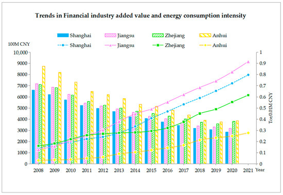
Figure 1.
The trend of financial industry added value and energy consumption intensity in the Yangtze River Delta region from 2008 to 2021. Data source: National Bureau of Statistics of China.
Concurrently, the financial industry’s added value demonstrated a continual upward trend, with the order of financial industry added value as follows: Jiangsu Province > Shanghai > Zhejiang Province > Anhui Province.
3.2. The Spatial Distribution of Financial Agglomeration and Carbon Emissions
In this study, we utilized ArcGIS 10.8 software to conduct spatial visualization analysis on the degree of financial agglomeration and CEI for the years 2008, 2013, and 2019. The detailed methods and sources of data are expounded in Section 3.
Figure 2 illustrates the uneven spatial distribution of CEI and financial agglomeration within China’s YRD region. The uneven distribution features of financial agglomeration are reflected in the high values of financial agglomeration (depicted in red) being concentrated in cities neighboring the southeastern coastal region of the YRD, namely Shanghai, Suzhou, Wuxi, Ningbo, Wenzhou, and Hangzhou. This concentration is linked to the construction plan of Shanghai as an international financial center. Moreover, the spatial disparities in carbon emissions are reflected in the lower values of carbon intensity (highlighted in dark green) being predominantly found in provincial capitals (Shanghai, Nanjing, Hangzhou, Hefei). China’s fiscal tradition of upward centralization has resulted in a significantly higher proportion of government resources in provincial capitals compared to other cities in the province. As a result, provincial capitals prioritize government emission reduction policies, leading to lower carbon emissions than in other cities.
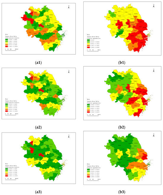
Figure 2.
Spatial distribution characteristics of financial agglomeration and carbon emission intensity in the Yangtze River Delta. (a1) represents the carbon emission intensity distribution among 41 cities in 2008; (a2) represents the distribution in 2013; and (a3) represents the distribution in 2019. Similarly, (b1) indicates the financial concentration distribution by city in 2019; (b2) indicates the distribution in 2013; and (b3) indicates the distribution in 2008.
In addition, from Figure 2(a1–a3), the number of green areas increases (low-CEI areas), and the red areas decrease (high-carbon-emission areas), revealing a declining trend in carbon emissions across the 41 cities in the YRD from 2008 to 2019. This trend is more pronounced in provincial capitals. From Figure 2(b1–b3), the transition of region colors from green areas (indicative of low financial agglomeration) to yellow and red regions (which indicate high financial agglomeration) signify an incremental trend in financial agglomeration degree. The more uniform color distribution reflects a deepening level of financial agglomeration and a narrowing gap from 2008 to 2019. Generally, the index of financial agglomeration is concentrated in Shanghai, slowly diminishing toward neighboring cities, while CEI exhibits a spatial distribution pattern that increases from provincial capitals toward the periphery.
Therefore, the analysis in this section indicates there is an uneven spatial geographical dispersion of carbon emissions and financial development within the YRD region of China.
3.3. Theoretical Mechanism and Research Hypotheses
The environmental Kuznets curve (EKC) suggests that environmental quality will initially degrade as a country’s economy grows but will subsequently improve once the economy reaches a certain level of income; there is a flipped U curve relationship between income and pollution [2,3,53,54]. In the agglomeration’s initial phases in the financial industry, historical factors, including the emphasis on heavy industry development at the inception of the People’s Republic of China and the use of GDP growth as a primary promotion metric for evaluating government officials [9], led financial institutions to give priority to short-term gains over long-term environmental sustainability. Consequently, investments were directed toward GHG-intensive industries, such as electric power, petrochemicals, building materials, and steel, resulting in a rise in fossil fuel consumption and subsequent carbon emissions. Additionally, the concentration of financial activities in urban areas contributed to urbanization and expansion, leading to higher energy consumption for transportation and infrastructure development. This, in turn, heightened the carbon emissions associated with increased car usage and energy consumption in densely populated areas.
As financial agglomeration reaches a certain threshold, it stimulates investment in facilitating the transition of GHG-intensive firms to renewable energy, thereby reducing carbon emissions [55,56]. Firstly, the clustering of financial industries can enhance economic efficiency through knowledge and technology spillovers. This efficiency has the potential to drive investments in clean technologies, thereby mitigating carbon emissions. Secondly, financial industry agglomeration can facilitate the regional coordination of emission reduction policies. This includes the development and adoption of information disclosure standards aligned with sustainable finance principles, aiming to bridge the information gap in sustainability data and regulatory measures. Moreover, by improving the availability and direction of sustainable financial instruments, such as green credit, green bonds, and green funds, firms with high greenhouse gas emissions can be incentivized to transition toward more sustainable practices, thereby reducing carbon emissions.
In summary, there may be a Kuznets curve relationship between the agglomeration of finance and carbon emissions; this paper posits Hypothesis H1.
H1.
Financial agglomeration exhibits an inverted U-shaped relationship with carbon emission intensity.
The spatial spillover effect refers to how an independent variable in neighboring regions influences the independent variable in the local region [57]. This influence may arise from the presence of spatial autocorrelation [58]. Previous research has shown the presence of spatial autocorrelation characteristics in carbon emissions [59], indicating that there is a spatial spillover effect between financial agglomeration and carbon emissions.
On the one hand, financial agglomeration precipitates spatial economic restructuring, which, in turn, alters the need for energy usage and pollution discharges within the area. The trade liberalization resulting from financial agglomeration triggers a regional transfer effect on carbon emissions, and stringent environmental regulations may prompt the relocation of polluting industries, which could potentially exacerbate ecological degradation in specific regions [60,61]. On the other hand, financial agglomeration enhances financial services’ capacity through inter-regional cooperation, such as support for clean energy R&D, the fostering of innovation in green technologies, and the design of financial instruments for emission reduction projects [35]. As financial agglomeration advances and emission reduction policies become more widespread, local governments will coordinate pollution control efforts, and financial services will radiate to surrounding cities. Ultimately, this concerted effort will propel the entire region toward carbon emission reduction. Considering this, Hypothesis H2 is posited.
H2.
Financial agglomeration exhibits a spatial spillover negative effect on carbon emissions.
Financial agglomeration has significantly enhanced the mobility of production factors, professional management knowledge, and technology, consequently leading to heightened competition among enterprises. However, this progress is tempered by governmental pollution regulations and market dynamics, which often cause the financial sector to reduce its investment toward high-pollution and high-energy-consumption (H&H) enterprises compared to green and low-carbon industries [50,62]. This dynamic interplay leads to the gradual elimination of H&H industries, such as GHG-intensive enterprises, within financial agglomeration regions or drives their transition toward low-carbon practices. As per the traditional three-sector division outlined in industrial economic theory, the secondary sector encompasses mining, electricity, manufacturing, and water and gas production and supply, along with construction, all of which host numerous GHG-intensive enterprises. Through financial agglomeration, funding can be channeled to facilitate the low-carbon transformation of these enterprises. Consequently, we posit Hypothesis H3.
H3.
Financial agglomeration facilitates industrial transformation by decreasing the share of the secondary industry, consequently mitigating carbon emissions.
4. Materials and Methods
4.1. Establishing an Assessment Framework for Financial Agglomeration Indicators
Given the data availability and the distinctive features of financial agglomeration in the YRD region, the empirical study selected panel data from the YRD region’s 41 cities spanning the years from 2008 to 2019. Given the absence of a unified index for measuring the level of financial agglomeration, building upon previous research, this paper examines financial agglomeration through three dimensions: financial scale, financial density, and financial depth. Specifically, financial scale represents the total financial capacity of a region; financial depth signifies the level of financial development; and financial density reflects the vitality of the financial system.
Drawing from the research methods of Tan, et al. [63] and Zou, et al. [64], we construct a financial agglomeration evaluation index framework. Subsequently, we calculate the degree of financial agglomeration using the entropy weight method with Stata 16 software. The specific index selection and attributes are detailed in Table 1. Among them, the number of financial institutions, the balance of financial institutions’ loans and deposits, and the number of financial workers are all sourced from Choice Financial Terminal. To mitigate the impact of inflation, we first obtain consumer price index (CPI) data for the years 2008 to 2019, which use the last year as the base period. These data are sourced from the Local Statistical Bureau and the China City Statistical Yearbook (CCSY). Next, using 2008 as the base year, we calculate the cumulative correction index. Finally, the balance of deposits and loans is divided by the correction index. The same methodology is applied to process the GDP data. The regional area, the regional population, and the proportion of tertiary industries’ added value data are sourced from the CCSY, China Economic Network statistical database, and EPS global statistical data. In addition to dimensionless treatment, the data undergo standardization.

Table 1.
Index framework for assessing the degree of financial agglomeration in the Yangtze River Delta.
4.2. Variable Setting
The dependent variable is CEI (variable code: cei). Following the methodology outlined in the existing literature, it is computed as the ratio of urban CO2 emissions to regional GDP, where GDP is adjusted for real values after excluding price factors. The China Carbon Accounting Database provides the source of CO2 emission data, with some cities requiring interpolation for missing emission data. For robustness testing, we use lnemission to replace cei, obtained by taking the logarithm of carbon emissions.
The independent variable is financial agglomeration (fin_agg). The mediating variable is industrial structure (ins), which is determined as the secondary industry’s added value as a percentage of GDP and serves as the mediating variable.
Control variables include economic development level (lngdp), calculated by taking the logarithm of GDP; green technology innovation (lngreen), represented by the logarithm of the number of green patents granted, with patent data sourced from the China Research Data Services Platform; urbanization rate (urban), as population urbanization is significantly inversely correlated with atmospheric pollution, measured by the percentage of people living in cities; and population density (lndp). Considering that denser populations tend to generate more carbon emissions in the long term, this paper uses the natural logarithm of population density, measured by population per square kilometer.
In conclusion, the panel data compiled in this article encompass 41 cities over an 11-year period from 2008 to 2019. The statistical values of the variables are shown in Table 2, with a notable observation that the standard deviation of cei is substantial, suggesting considerable variability in CEI values around the mean. Additionally, the range of fin_agg spans from 0 to 1, indicating a wide dispersion in the degree of financial agglomeration values.
Table 2.
Descriptive statistics of key variables.
4.3. Model Design and Empirical Strategies
4.3.1. Benchmark Model
This study employs the panel fixed effects model to examine the nonlinear correlation between financial agglomeration and CEI. The extremities of the nonlinear relationship are assessed through grouping regression analysis.
where cei represents the CEI. fin_agg indicates the degree of regional financial agglomeration; t and i in the equations above represent years and cities, respectively. represents the control variable. is the fixed effect of the city. is the fixed effect of the year. is the residual item. is a constant item. The benchmark model controls both time and municipal fixed effects and adopts the robust standard error clustered to the municipal level.
4.3.2. Spatial Durbin Model
This study uses the spatial panel model for regression and establishes the following three spatial econometric models: the spatial lag model (SAR) is represented by Equation (2), the spatial error model (SEM) by Equation (3), and the spatial Durbin model (SDM) by Equation (4) [65].
where and are the city and year, is the explanatory variable CEI, is a series of variables including the explanatory variables of the financial agglomeration degree and control variables, is the spatial lag term coefficient, is the spatial autoregressive coefficient of the spatial error term, and and are the parameters to be estimated in the model. Whether the SDM can be simplified to the spatial error or spatial lag model needs to be tested on two assumptions. Hypothesis 1 is —it is possible to determine whether to reduce the spatial Durbin to spatial lag, and Hypothesis 2 is —it is possible to determine whether to simplify the SDM to the spatial error model.
, is a standardized non-negative spatial weight matrix of N × N dimension, and is a measure of spatial autocorrelation.
The spatial weight matrix W is the coefficient matrix of the correlation between the two regions. In this study, is the geographical distance matrix, is the inverse distance spatial weight matrix, and all W matrices are standardized. The difference between and is that is built using Cartesian coordinates for latitude and longitude, and is built using spherical coordinates and specifies a radius of 3958.761 miles from Earth.
The inverse distance spatial weight matrix takes the following form:
In Equation (6), d represents the spherical distance between regions i and j.
In this paper, is the binary space weights matrix of adjacencies; the form is as follows:
In Equation (7), if two places are adjacent, then the corresponding element in the weight matrix is taken as 1 for and 0 for vice versa.
Due to the spatial correlation, the total effect of exogenous variables in the spatial econometric model can be decomposed into direct effects; the former refers to the impact of the change in the exogenous variable of region i on the explanatory variable of region i after considering the spatial correlation, and the latter represents the effect of the change in exogenous variables in other regions -i on the explanatory variable of region i. Both can be obtained by using the explanatory variable to find the partial derivative of the explanatory variable.
Equation (8)—41 is the (i,j) element of the spatial weight matrix W.
4.3.3. Mechanism Test Model
This paper tests the mediating mechanism by referencing Khan, et al. [66] to examine the process by which financial agglomeration lowers CEI. Firstly, we construct a regression model (9), which is derived from Equation (4), with the industrial structure level (ins) as the dependent variable and financial agglomeration (fin_agg) is the independent variable, to test the impact of financial agglomeration on industrial structures. Secondly, ins and fin_agg are included in the model (10). shows the mediating effect of industrial structure adjustment. If it is significant, then H3 is verified.
5. Empirical Results and Analysis
5.1. Nonlinear Relationship Analysis
5.1.1. Model Testing
Before conducting regression analysis, several tests were performed on the panel data (shown in Table 3). Firstly, the HT and LM tests yielded a significant p-value of 0, suggesting the absence of unit roots in the panel data. Next, the F-test resulted in a p-value (Prob > F is 0) of significantly 0, suggesting that the fixed effects model is more appropriate than the regression model of ordinary least squares (OLS). Thirdly, the p-value generated by the Hausman test is significant at 0; to address the risk of the Hausman test being ineffective in the presence of heteroscedasticity and autocorrelation, we supplemented the Hausman test based on the bootstrap method. The p-value generated by the bootstrap Hausman test is also 0 at the 10% significance level, demonstrating that the fixed effects model outperforms the random effect model. Furthermore, considering that explanatory variables such as financial agglomeration and GDP population are influenced by time factors and exhibit varying trends across different cities, a bidirectional fixed effects model, accounting for both temporal and regional effects, was selected for regression in this study.
Table 3.
Model selection test results.
5.1.2. Nonlinear Relation Test
Column (1) in Table 4 presents the regression findings from the two-way fixed effects model. In this model, the coefficient for fin_agg is 18.978, and the coefficient for the squared term fin_agg2 representing financial agglomeration is −10.707. There is an evident inverted U-shaped relationship between financial agglomeration and CEI, as both p-values pass the significance level test of 5%. This shows that a Kuznets curve exists between financial agglomeration and carbon emissions. On the one hand, during periods of low financial agglomeration, financial institutions often prioritize immediate profits over enduring sustainable development. This tendency results in increased investments in heavy industry, resulting in higher energy consumption and, consequently, elevated carbon emissions. On the other hand, heightened financial agglomeration fosters knowledge and technology spillovers, thereby enhancing economic efficiency. This efficiency encourages investments in clean technologies, consequently reducing carbon emissions. Thus, the U test (Lind and Mehlum [33]) results in Table 5 point to two conclusions. Firstly, the extreme point of the inverted U curve falls at 0.651, within the range of fin_agg values [0.010, 0.943]. However, it is noted that only Shanghai has achieved a financial agglomeration level of 0.651. Secondly, at the 5% significance level, the null hypothesis (monotone or inverse U shape) is rejected, with a negative sign observed in the interval for the slope, evidencing an inverted U-shaped link between financial agglomeration and carbon emissions again. Moreover, based on the extremum point, the sample is categorized into two groups (group 1: fin_agg < 0.651, group 2: fin_agg > 0.651). The regression results presented in columns (2) and (3) of Table 4 display coefficients for fin_agg of 7.912 and −1.659, respectively. These coefficients reveal that when financial agglomeration is below 0.651, inter-city financial agglomeration exacerbates carbon emissions per unit of GDP. Conversely, when the inter-city financial agglomeration level exceeds 0.651, financial agglomeration reduces CEI. Consequently, Hypothesis H1 is validated.
Table 4.
Results of the nonlinear regression.
Table 5.
Results of U test.
5.2. Spatial Spillover Analysis
5.2.1. Spatial Autocorrelation Test
Before using spatial econometric models for estimation, conducting a spatial correlation test on the carbon emissions of the 41 cities in the YRD is essential. Table 6 displays the values for Moran’s I (see Equation (5)). The global spatial autocorrelation index (Moran’s I) of the total carbon emissions for each year in urban areas is consistently positive and must pass the significance test of 5%.
Table 6.
The Moran index of carbon emissions in the Yangtze River Delta region from 2008 to 2019.
Figure 3 presents a scatter plot of the Moran index. Within Figure 3, cities are predominantly clustered in the first and third quadrants, suggesting that CO2 emissions tend to move in the same direction among adjacent cities. Cities in the third quadrant suggest that the carbon emissions gap between the city and its neighboring cities is relatively small, while those in the first quadrant indicate a larger carbon emission gap with neighboring cities. Anhui Province’s 16 cities (26~41) are mainly concentrated in the third quadrant, as the economic development in Anhui Province is led by the provincial capital, resulting in relatively small economic disparities among cities within the province and, consequently, smaller differences in carbon emissions. The cities in the first quadrant include Shanghai, Ningbo, Jiaxing, Changzhou, Suzhou, and Shaoxing. These cities, characterized by rapid development and high energy consumption, exhibit significantly higher total carbon emissions than other cities.
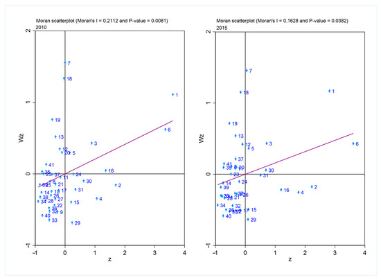
Figure 3.
Scatter plot of the Moran index of carbon emissions in 2010 and 2015. The numbers 1–41 represent the following: 1—Shanghai, 2—Nanjing, 3—Wuxi, 4—Xuzhou, 5—Changzhou, 6—Suzhou, 7—Nantong, 8—Lian-yungang, 9—Huai’an, 10—Yancheng, 11—Yangzhou, 12—Zhenjiang, 13—Taizhou, 14—Suqian, 15—Hangzhou, 16—Ningbo, 17—Wenzhou, 18—Jiaxing, 19—Huzhou, 20—Shaoxing, 21—Jinhua, 22—Quzhou City, 23—Zhoushan, 24—Taizhou, 25—Lishui, 26—Hefei, 27—Wuhu, 28—Bengbu, 29—Huainan city, 30—Ma’ anshan, 31—Huaibei, 32—Tongling, 33—Anqing, 34—Huangshan, 35—Chuzhou, 36—Fuyang, 37—Su-zhou city, 38—Lu’ an, 39—Bozhou city, 40—Chizhou, 41—Xuan city.
The above analysis suggests a strong positive spatial correlation in CEI, necessitating the construction of spatial econometric models for accurate estimation.
5.2.2. Selection of Spatial Panel Econometric Models
The statistical values and significance of the LM and robust LM tests were used to make the initial decision regarding the adoption of a spatial panel model in the lag or error term when choosing spatial econometric models. The categories of spatial econometric models are illustrated in Figure 4, and the outcomes of the examination are presented in Table 7. The estimation results revealed that the statistics for LM spatial error, robust LM spatial error, LM spatial lag, and robust LM spatial lag all passed the 5% significance level test, indicating that both the spatial lag and spatial error terms concurrently impact the model. Further verification of whether SDM can degrade to the spatial lag model (SLM) or spatial error model (SEM) was conducted through the statistical tests for LR spatial lag, LR spatial error, Wald spatial lag, and Wald spatial error, with all passing the 5% significance level test. These results reject the null hypothesis, confirming that the panel SDM is the optimal model. The subsequent application of the Hausman test to choose between fixed effects and random effects yielded a Hausman index of 76.44. The index passed the 1% significance test, indicating the suitability of fixed effects. The fixed effects in the SDM include temporal fixed effects, spatial fixed effects, and spatiotemporal dual fixed effects. The joint significance of the LR test for the spatiotemporal dual fixed effects concerning the financial agglomeration index on carbon emissions suggests that spatiotemporal dual fixed effects outperform temporal and spatial fixed effects. Consequently, the SDM with spatiotemporal dual fixed effects was selected to investigate the influence of YRD financial agglomeration on carbon emissions.
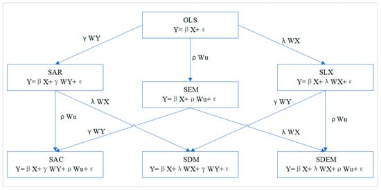
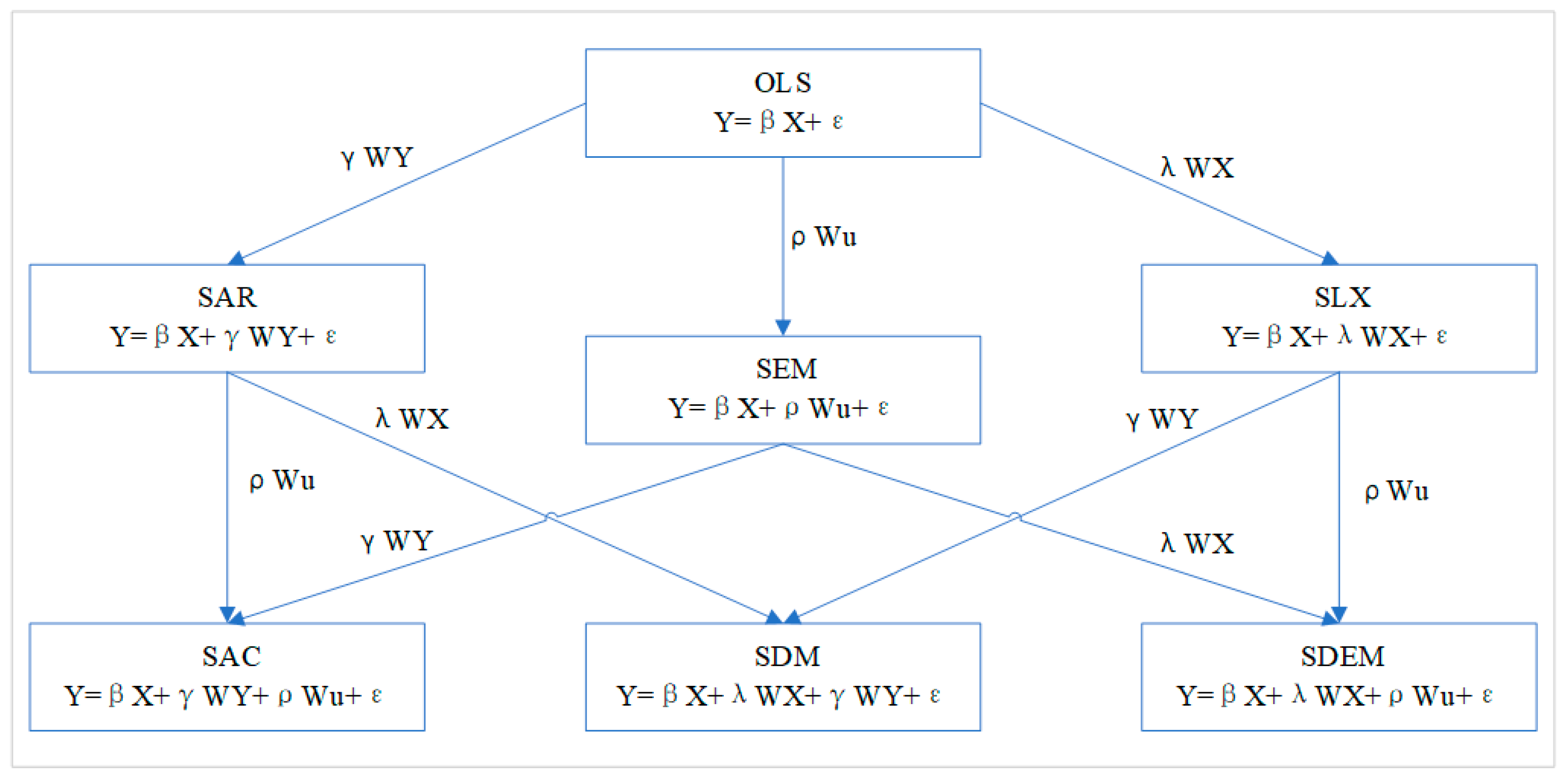
Figure 4.
Types and relationships of space panel measurement models. SAR—spatial lag model, SLX—spatial lag model with exogenous variables, SAC—spatial autoregressive conditionally heteroskedastic model, and SDEM—spatial Durbin error model.
Table 7.
Results of the spatial measurement model identification tests.
5.2.3. Spatial Spillover Effect Test Results
Utilizing Stata 16.0 software, we conducted SDM with spatiotemporal double fixed effects to estimate spatial spillover effects based on the panel data in the YRD region. The results are summarized in Table 8.
Table 8.
The spatial Durbin model regression results.
From the data reported in Table 8, we can derive the following two conclusions:
Firstly, considering spatial effects, the inverted U-shaped relationship still persists. The first-order term coefficient (fin_agg) for financial agglomeration in Column (1) is significant at 15.946, and the coefficient for the quadratic term (fin_agg2) is also significant at . According to the estimation model, the maximum point for carbon emissions is at fin_agg, equal to 0.76 (. This indicates that when fin_agg < 0.76, a 1% increase in fin_agg will lead to a 15.8% increase in urban CEI (Column 1), whereas when fin_agg > 0.76, this will result in a 15.8% decrease in CEI. This analysis suggests that the impact of financial agglomeration on urban CEI in the YRD follows a nonlinear inverted U-shaped relationship. The research findings reconfirm the validity of H1.
Secondly, financial agglomeration exhibits negative spatial spillover effects on carbon emissions, indicating the positive externalities associated with financial agglomeration. That is, the concentration of financial activities in one area can mitigate carbon emissions in surrounding regions. Columns (1), (2), and (3) in Table 8, respectively, display the outcomes of the SDM regression with the geographic distance weight matrix (), binary spatial weight matrix of geographic adjacency relations (), and inverse distance spatial weight matrix (). The spatial spillover effects (-values) of financial agglomeration on carbon emissions are , respectively. Moreover, they pass significance tests at least at the 10% level, indicating the presence of spatial spillover negative effects from financial agglomeration on carbon emissions. In other words, this demonstrates the positive externality of financial agglomeration. The ρ value in Column (1) is −1.163, suggesting that a 1% increase in local financial agglomeration leads to a 1.163% reduction in CEI in surrounding areas. Additionally, the coefficients for Wx:fin_agg are , indicating that financial agglomeration in neighboring cities decreases the CEI in the local city.
In summary, the local development of financial agglomeration reduces the CEI in surrounding cities, while the development of financial agglomeration in neighboring cities also decreases the CEI in the local city. The impact of financial agglomeration on CEI exhibits significantly negative spatial spillover effects, proving that H2 is verified.
5.2.4. Spatial Spillover Effect Decomposition
To further examine the marginal effects of financial agglomeration development on carbon emissions in the YRD region, we employed the matrix to decompose spatial effects, revealing the influence of financial agglomeration on both local and adjacent areas’ CEI through direct and spillover effects (the results are presented in Table 9).
Table 9.
Decomposition results of spatial spillover effects.
Regarding the direct effects, the quadratic term (fin_agg2) has a significantly negative coefficient, but the fin_agg linear term has a significantly positive coefficient. This indicates that the impact of financial agglomeration on local CEI increases initially and then decreases. Regarding spillover effects, the coefficient of fin_agg is negative and significant, while the quadratic term is positive but not significant. This suggests that an increase in local financial agglomeration reduces the CEI of surrounding cities. Additionally, with |−26.043|>|15.642| in Table 8, the indirect effect outweighs the direct effect, revealing that financial agglomeration development has a positive effect in inhibiting carbon emissions in surrounding cities. Considering the overall effect, the coefficient is −10.401, significant at the 10% level. The aforementioned findings suggest that the development of financial agglomeration can lead to a reduction in carbon emissions through spatial spillover effects.
5.2.5. Robustness Test
The logarithm of total carbon emissions (lnemission) in this study is utilized as a proxy variable for carbon emissions, and robustness tests are conducted (Table 10). The coefficients of the fin_agg first- and second-order terms are positive and negative, respectively, demonstrating an inverted U-shaped relationship between the two variables, confirming H1. The negative value indicates a spatial spillover negative effect. The direct effect coefficients of fin_agg2 are −1.670, −1.026, and −1.089, respectively, with the overall effect coefficient being negative. This suggests that financial agglomeration development has a spatial effect on suppressing carbon emissions, confirming H2. Hence, the empirical conclusions in this paper are robust.
Table 10.
Robustness test.
5.3. Verification of Mechanism
Columns (1) and (2) in Table 11 display the regression results for the mechanism identification models (Equations (9) and (10)) in Section 4.3. Firstly, the regression coefficient between the financial agglomeration variable (fin_agg) and the industrial structure variable (ins) is and is significant at the 1% level, pointing to a negative correlation between financial agglomeration and the share of added value from the secondary industry in the total GDP. This implies that the development of financial agglomeration in the YRD can reduce the percentage of the secondary industry. Secondly, the indirect effect is equal to (), suggesting that for each 1% increase in financial agglomeration, CEI can decrease by 3.62% units due to industrial transformation efforts aimed at decreasing the share of the secondary sector. This is because the intensification of competition, technological spillovers, and financial support brought about by financial agglomeration can drive the demand for low-carbon transformation among GHG-intensive firms in such industries. The study concludes that the development of financial agglomeration reduces CEI, through industrial transformation, to lower the share of the secondary industry, verifying Hypothesis H3.
Table 11.
Mechanism testing.
The hypothesis testing outcomes of this study, as summarized in Table 12, confirm that all hypotheses are supported.
Table 12.
Hypothesis test results.
6. Conclusions and Recommendations
6.1. Conclusions
Whether the development of financial agglomeration in China can contribute to attaining the objectives of “carbon peak” and “carbon neutrality” is a topic worthy of investigation. This paper, using panel data from 41 cities in the YRD from 2008 to 2019, examines the effect of financial agglomeration on carbon emissions, as well as its spatial spillover effects and the underlying mechanisms. The key findings are as follows.
Firstly, we analyzed the spatiotemporal distribution of financial agglomeration and carbon emissions in the YRD. Over the sample period, carbon emissions in this area have been decreasing while the number of financial institutions has been increasing. Financial agglomeration is concentrated in southeastern coastal areas, such as Shanghai, Suzhou, Wuxi, Ningbo, Wenzhou, and Hangzhou. The quantity of financial institutions decreases progressively from Shanghai to the surrounding cities, whereas carbon emissions exhibit an increasing trend from provincial capital cities to peripheral cities. In summary, there is an uneven spatial distribution in both financial agglomeration and carbon emissions.
Secondly, employing a benchmark model, we verified a significant inverted U-shaped nonlinear relationship between the degree of financial agglomeration and CEI. The critical point occurs at a financial agglomeration level of 0.651. Therefore, when the financial agglomeration exceeds 0.651, it is associated with the suppression of carbon emissions. However, currently, Shanghai is the only city that has achieved this level of financial agglomeration.
Thirdly, using an SDM, we verified the spatial spillover negative effects of financial agglomeration on carbon emissions. Financial agglomeration in neighboring cities suppresses local carbon emissions, whereas local financial agglomeration decreases carbon emissions in neighboring cities. Spatial effect decomposition shows that the indirect effect exceeds the direct effect, with an overall negative impact, suggesting a stronger suppressive effect on external carbon emissions compared to local emissions.
Fourthly, our mechanism study has found that financial agglomeration reduces carbon emissions by promoting industrial transformation, specifically by decreasing the proportion of secondary industry.
6.2. Policy Recommendations
Drawing on the conclusions outlined in this study, we put forward the following recommendations. Firstly, we suggest that Chinese governments need to break down administrative barriers and strengthen regional economic and financial cooperation, as well as implement emission reduction policies collaboratively. Implementing tailored financial development and emission reduction strategies based on local conditions is essential. Emphasis should be placed on enforcing environmental regulations in regions characterized by underdeveloped financial sectors. This approach aims to mitigate the early-stage negative impact of financial concentration on carbon emissions.
Secondly, China needs to narrow the regional disparities in financial development and strengthen an inclusive financial system. We recommend that China supports the establishment of integrated financial institutions. The financial sector should learn from the financial development experience of Shanghai, assisting cities with lower levels of financial development in enhancing their financial service capabilities. Financial institutions should aggressively advance green finance, develop novel carbon-hedging instruments and products, enhance the liquidity of carbon financial products, and strengthen the spillover dividends of financial agglomeration.
Thirdly, to fully leverage the positive externality of financial agglomeration spatial spillover effects, it is imperative for financial institutions, real enterprises, and scientific research institutions to coordinate their geographical locations. This coordination would aim to facilitate the integrated development of industries. This could involve establishing large industrial zones to form cross-regional industrial chains, further developing an interconnected high-speed rail and internet network, piloting cross-regional joint credit initiatives, enhancing mobile payment capabilities, and creating a shared platform for cross-regional public credit information. Furthermore, expanding the scope of carbon emission trading pilots and establishing a unified large-scale carbon trading market are crucial steps in advocating for cross-regional collaborative governance over carbon emissions.
Lastly, as financial agglomeration may cause secondary industries to decline in shares to mitigate carbon emissions, China needs to encourage the green transformation of the secondary industry, especially capital investment in the transformation of GHG-intensive industries. China should enhance investments in digitalization and intelligent R&D, empower advanced manufacturing, and boost high-end service industries. Encouraging support from venture capital funds and private equity funds for investments in green enterprises is essential. Establishing a repository of green development projects and reinforcing major technological breakthroughs and applications in green and low-carbon technologies is imperative.
The main limitations of this study are as follows. Firstly, China has 293 prefecture-level cities, contributing to approximately 60% of global carbon emissions from fossil fuels. Reducing carbon emissions across China is crucial. Nevertheless, because of limitations in data availability, this study focused on 41 of these prefecture-level cities. Secondly, this paper solely investigated the potential of financial agglomeration to decrease the proportion of secondary industries, thereby mitigating carbon emissions. Alternative avenues for emission reduction have not been explored. In the future, with access to additional data, we will aim to investigate whether the conclusions drawn in this paper regarding the impact of financial agglomeration on carbon emissions hold true on a national level. We also intend to comprehensively explore the underlying mechanisms and formulate more generalized recommendations.
Author Contributions
Conceptualization, Q.H.; methodology, Q.H.; software, Q.H.; validation, Q.H.; formal analysis, Q.H.; data curation, Q.H.; writing—original draft preparation, Q.H. and Y.H.; writing—review and editing, Q.H.; visualization, Q.H.; supervision, A.S.; project administration, A.S.; funding acquisition, A.S. All authors have read and agreed to the published version of the manuscript.
Funding
This research was supported by the Major Project of the National Social Science Foundation ’Research on Preventing and Responding to Foreign Economic Sanctions under the Concept of Overall National Security’ of China (NO. 22&ZD180), the Ministry of Education Project of China (NO. 23YJA790068).
Institutional Review Board Statement
Not applicable.
Informed Consent Statement
Not applicable.
Data Availability Statement
The data presented in this study are available from the corresponding author, Qun He, upon reasonable request.
Conflicts of Interest
The authors declare no conflicts of interest.
References
- Manioudis, M.; Meramveliotakis, G. Broad Strokes towards a Grand Theory in the Analysis of Sustainable Development: A Return to the Classical Political Economy. New Polit. Econ. 2022, 27, 866–878. [Google Scholar] [CrossRef]
- Arrow, K.; Bolin, B.; Costanza, R.; Dasgupta, P.; Folke, C.; Holling, C.S.; Jansson, B.O.; Levin, S.; Maler, K.G.; Perrings, C.; et al. Economic Growth, Carrying Capacity, and the Environment. Science 1995, 268, 520–521. [Google Scholar] [CrossRef]
- Panayotou, T. Environmental Degradation at Different Stages of Economic Development. In Beyond Rio; Ahmed, I., Doeleman, J.A., Eds.; Palgrave Macmillan: London, UK, 1995; pp. 13–36. ISBN 978-1-349-24247-4. [Google Scholar]
- Matthews, H.D.; Wynes, S. Current Global Efforts Are Insufficient to Limit Warming to 1.5 °C. Science 2022, 376, 1404–1409. [Google Scholar] [CrossRef]
- Liu, Z.; Deng, Z.; He, G.; Wang, H.; Zhang, X.; Lin, J.; Qi, Y.; Liang, X. Challenges and Opportunities for Carbon Neutrality in China. Nat. Rev. Earth Environ. 2022, 3, 141–155. [Google Scholar] [CrossRef]
- Meramveliotakis, G.; Manioudis, M. Default Nudge and Street Lightning Conservation: Towards a Policy Proposal for the Current Energy Crisis. J. Knowl. Econ. 2023, 1–10. [Google Scholar] [CrossRef]
- Chu, S.; Majumdar, A. Opportunities and Challenges for a Sustainable Energy Future. Nature 2012, 488, 294–303. [Google Scholar] [CrossRef] [PubMed]
- Law, S.; Singh, N. Does Too Much Finance Harm Economic Growth? J. Bank. Financ. 2014, 41, 36–44. [Google Scholar] [CrossRef]
- Zhang, X.; Cheng, X. Energy Consumption, Carbon Emissions, and Economic Growth in China. Ecol. Econ. 2009, 68, 2706–2712. [Google Scholar] [CrossRef]
- Soytas, U.; Sari, R. Energy Consumption, Economic Growth, and Carbon Emissions: Challenges Faced by an EU Candidate Member. Ecol. Econ. 2009, 68, 1667–1675. [Google Scholar] [CrossRef]
- Narayan, P.; Narayan, S. Carbon Dioxide Emissions and Economic Growth: Panel Data Evidence from Developing Countries. Energy Policy 2010, 38, 661–666. [Google Scholar] [CrossRef]
- Alam, M.; Murad, M.; Nornanc, A.; Ozturk, I. Relationships among Carbon Emissions, Economic Growth, Energy Consumption and Population Growth: Testing Environmental Kuznets Curve Hypothesis for Brazil, China, India and Indonesia. Ecol. Indic. 2016, 70, 466–479. [Google Scholar] [CrossRef]
- Bekun, F.; Emir, F.; Sarkodie, S. Another Look at the Relationship between Energy Consumption, Carbon Dioxide Emissions, and Economic Growth in South Africa. Sci. Total Environ. 2019, 655, 759–765. [Google Scholar] [CrossRef]
- Al-Mulali, U.; Ozturk, I.; Lean, H. The Influence of Economic Growth, Urbanization, Trade Openness, Financial Development, and Renewable Energy on Pollution in Europe. Nat. Hazards 2015, 79, 621–644. [Google Scholar] [CrossRef]
- Rahman, M.; Kashem, M. Carbon Emissions, Energy Consumption and Industrial Growth in Bangladesh: Empirical Evidence from ARDL Cointegration and Granger Causality Analysis. Energy Policy 2017, 110, 600–608. [Google Scholar] [CrossRef]
- Fang, Z.; Gao, X.; Sun, C. Do Financial Development, Urbanization and Trade Affect Environmental Quality? Evidence from China. J. Clean. Prod. 2020, 259, 120892. [Google Scholar] [CrossRef]
- Gao, D.; Li, Y.; Tan, L. Can Environmental Regulation Break the Political Resource Curse: Evidence from Heavy Polluting Private Listed Companies in China. J. Environ. Plan. Manag. 2023, 1–27. [Google Scholar] [CrossRef]
- Ahmed, K.; Bhattacharya, M.; Shaikh, Z.; Ramzan, M.; Ozturk, I. Emission Intensive Growth and Trade in the Era of the Association of Southeast Asian Nations (ASEAN) Integration: An Empirical Investigation from ASEAN-8. J. Clean. Prod. 2017, 154, 530–540. [Google Scholar] [CrossRef]
- Costa, L.; Moreau, V. The Emission Benefits of European Integration. Environ. Res. Lett. 2019, 14, 084044. [Google Scholar] [CrossRef]
- Kim, D.; Wu, Y.; Lin, S. Carbon Dioxide Emissions and the Finance Curse. Energy Econ. 2020, 88, 104788. [Google Scholar] [CrossRef]
- Wang, Y.; Yin, S.; Fang, X.; Chen, W. Interaction of Economic Agglomeration, Energy Conservation and Emission Reduction: Evidence from Three Major Urban Agglomerations in China. Energy 2022, 241, 122519. [Google Scholar] [CrossRef]
- Zhang, M.; Liu, Y. Influence of Digital Finance and Green Technology Innovation on China’s Carbon Emission Efficiency: Empirical Analysis Based on Spatial Metrology. Sci. Total Environ. 2022, 838, 156463. [Google Scholar] [CrossRef] [PubMed]
- Gao, D.; Tan, L.; Mo, X.; Xiong, R. Blue Sky Defense for Carbon Emission Trading Policies: A Perspective on the Spatial Spillover Effects of Total Factor Carbon Efficiency. Systems 2023, 11, 382. [Google Scholar] [CrossRef]
- Gao, D.; Feng, H.; Cao, Y. The Spatial Spillover Effect of Innovative City Policy on Carbon Efficiency: Evidence from China. Singap. Econ. Rev. 2024. [Google Scholar] [CrossRef]
- Chen, X.; Chen, Z. Can Green Finance Development Reduce Carbon Emissions? Empirical Evidence from 30 Chinese Provinces. Sustainability 2021, 13, 12137. [Google Scholar] [CrossRef]
- Li, Z.; Liu, W.; Wei, X. The Impact of Digital Finance Development on Carbon Dioxide Emissions: Evidence from Households in China. Technol. Forecast. Soc. Chang. 2023, 190, 122364. [Google Scholar] [CrossRef]
- Wang, J.; Tian, J.; Kang, Y.; Guo, K. Can Green Finance Development Abate Carbon Emissions: Evidence from China. Int. Rev. Econ. Financ. 2023, 88, 73–91. [Google Scholar] [CrossRef]
- Wang, T.; Umar, M.; Li, M.; Shan, S. Green Finance and Clean Taxes Are the Ways to Curb Carbon Emissions: An OECD Experience. Energy Econ. 2023, 124, 106842. [Google Scholar] [CrossRef]
- Gao, D.; Zhou, X.; Mo, X.; Liu, X. Unlocking Sustainable Growth: Exploring the Catalytic Role of Green Finance in Firms’ Green Total Factor Productivity. Environ. Sci. Pollut. Res. 2024. [Google Scholar] [CrossRef]
- Kindleberger, C.P. The Formation of Financial Centers: A Study in Comparative Economic History. Work. Pap. 1973, 5, 3395–3397. [Google Scholar]
- Shahbaz, M.; Shahzad, S.; Ahmad, N.; Alam, S. Financial Development and Environmental Quality: The Way Forward. Energy Policy 2016, 98, 353–364. [Google Scholar] [CrossRef]
- Setyowati, A.B. Governing Sustainable Finance: Insights from Indonesia. Clim. Policy 2023, 23, 108–121. [Google Scholar] [CrossRef]
- Lind, J.T.; Mehlum, H. With or Without U? The Appropriate Test for a U-Shaped Relationship*: Practitioners’ Corner. Oxf. Bull. Econ. Stat. 2010, 72, 109–118. [Google Scholar] [CrossRef]
- SASABUCHI, S. A Test of a Multivariate Normal Mean with Composite Hypotheses Determined by Linear Inequalities. Biometrika 1980, 67, 429–439. [Google Scholar] [CrossRef]
- Yuan, H.; Feng, Y.; Lee, J.; Liu, H.; Li, R. The Spatial Threshold Effect and Its Regional Boundary of Financial Agglomeration on Green Development: A Case Study in China. J. Clean. Prod. 2020, 244, 118670. [Google Scholar] [CrossRef]
- Porteous, D.J. The Geography of Finance: Spatial Dimensions of Intermediary Behaviour; Avebury: Aldershot, UK, 1995. [Google Scholar]
- Fujita, M.; Thisse, J.-F. Economics of Agglomeration: Cities, Industrial Location, and Regional Growth; Cambridge University Press: Cambridge, UK, 2002. [Google Scholar]
- Arthur, J.B. Effects of Human Resource Systems on Manufacturing Performance and Turnover. Acad. Manag. J. 1994, 37, 670–687. [Google Scholar] [CrossRef]
- Rosenthal, S.S.; Strange, W.C. Chapter 49—Evidence on the Nature and Sources of Agglomeration Economies. In Handbook of Regional and Urban Economics; Henderson, J.V., Thisse, J.-F., Eds.; Elsevier: Amsterdam, The Netherlands, 2004; Volume 4, pp. 2119–2171. ISBN 1574-0080. [Google Scholar]
- Acheampong, A.O. Modelling for Insight: Does Financial Development Improve Environmental Quality? Energy Econ. 2019, 83, 156–179. [Google Scholar] [CrossRef]
- Zhang, Y.-J.; Liu, Z.; Zhang, H.; Tan, T.-D. The Impact of Economic Growth, Industrial Structure and Urbanization on Carbon Emission Intensity in China. Nat. Hazards 2014, 73, 579–595. [Google Scholar] [CrossRef]
- Acheampong, A.O.; Amponsah, M.; Boateng, E. Does Financial Development Mitigate Carbon Emissions? Evidence from Heterogeneous Financial Economies. Energy Econ. 2020, 88, 104768. [Google Scholar] [CrossRef]
- Liu, H.; Song, Y. Financial Development and Carbon Emissions in China since the Recent World Financial Crisis: Evidence from a Spatial-Temporal Analysis and a Spatial Durbin Model. Sci. Total Environ. 2020, 715, 136771. [Google Scholar] [CrossRef] [PubMed]
- Liu, X.; Liu, X. Can Financial Development Curb Carbon Emissions? Empirical Test Based on Spatial Perspective. Sustainability 2021, 13, 11912. [Google Scholar] [CrossRef]
- Okere, K.I.; Onuoha, F.C.; Muoneke, O.B.; Oyeyemi, A.M. Towards Sustainability Path in Argentina: The Role of Finance, Energy Mix, and Industrial Value-Added in Low or High Carbon Emission—Application of DARDL Simulation. Environ. Sci. Pollut. Res. 2021, 28, 55053–55071. [Google Scholar] [CrossRef]
- He, J.; Iqbal, W.; Su, F. Nexus between Renewable Energy Investment, Green Finance, and Sustainable Development: Role of Industrial Structure and Technical Innovations. Renew. Energy 2023, 210, 715–724. [Google Scholar] [CrossRef]
- Hamed, W.M.A.; Özataç, N. Spillover Effects of Financial Development on Renewable Energy Deployment and Carbon Neutrality: Does GCC Institutional Quality Play a Moderating Role? Environ. Dev. Sustain. 2023. [Google Scholar] [CrossRef]
- Bai, J.; Chen, Z.; Yan, X.; Zhang, Y. Research on the Impact of Green Finance on Carbon Emissions: Evidence from China. Econ. Res.-Ekon. Istraživanja 2022, 35, 6965–6984. [Google Scholar] [CrossRef]
- Cui, S.; Wang, Z. The Impact and Transmission Mechanisms of Financial Agglomeration on Eco-Efficiency: Evidence from the Organization for Economic Co-Operation and Development Economies. J. Clean. Prod. 2023, 392, 136219. [Google Scholar] [CrossRef]
- Mei, B.; Ali, M.; Khan, I.; Luo, J. Analyzing the Mediating Role of Industrial Structure in the Spatial Spillover Effects of Financial Agglomeration on Carbon Emission and Regional Heterogeneity. Environ. Sci. Pollut. Res. 2023. [Google Scholar] [CrossRef] [PubMed]
- Yan, B.; Wang, F.; Dong, M.; Ren, J.; Liu, J.; Shan, J. How Do Financial Spatial Structure and Economic Agglomeration Affect Carbon Emission Intensity? Theory Extension and Evidence from China. Econ. Model. 2022, 108, 105745. [Google Scholar] [CrossRef]
- Fan, W.; Wang, F.; Liu, J.; Yan, B.; Chen, T.; Liu, S.; Zhang, H. Environmental Effects of Financial Agglomeration under Dual Correlations of Industry and Space: Evidence from 286 Prefecture-Level Cities in China. Environ. Impact Assess. Rev. 2023, 98, 106978. [Google Scholar] [CrossRef]
- Selden, T.; Daqing, S. Environmental Quality and Development: Is There a Kuznets Curve for Air Pollution Emissions? J. Environ. Econ. Manag. 1994, 27, 147–162. [Google Scholar] [CrossRef]
- Kuznets, S. Economic Growth and Income Inequality. Am. Econ. Rev. 1955, 45, 1–28. [Google Scholar]
- Yao, S.; Zhang, S.; Zhang, X. Renewable Energy, Carbon Emission and Economic Growth: A Revised Environmental Kuznets Curve Perspective. J. Clean. Prod. 2019, 235, 1338–1352. [Google Scholar] [CrossRef]
- Long, X.; Naminse, E.; Du, J.; Zhuang, J. Nonrenewable Energy, Renewable Energy, Carbon Dioxide Emissions and Economic Growth in China from 1952 to 2012. Renew. Sustain. Energy Rev. 2015, 52, 680–688. [Google Scholar] [CrossRef]
- LeSage, J.; Pace, R.K. Introduction to Spatial Econometrics, 1st ed.; Chapman and Hall/CRC: New York, NY, USA, 2009; ISBN 978-0-429-13808-9. [Google Scholar]
- Getis, A. Spatial Autocorrelation. In Handbook of Applied Spatial Analysis: Software Tools, Methods and Applications; Fischer, M.M., Ed.; Springer: Berlin/Heidelberg, Germany, 2010; pp. 255–275. ISBN 978-3-642-03646-0. [Google Scholar]
- Liu, Q.; Wu, S.; Lei, Y.; Li, S.; Li, L. Exploring Spatial Characteristics of City-Level CO2 Emissions in China and Their Influencing Factors from Global and Local Perspectives. Sci. Total Environ. 2021, 754, 142206. [Google Scholar] [CrossRef]
- Chen, Z.; Liu, Y.; Zhang, Y.; Zhong, Z. Inter-Regional Economic Spillover and Carbon Productivity Embodied in Trade: Empirical Study from the Pan-Yangtze River Delta Region. Environ. Sci. Pollut. Res. 2021, 28, 7390–7403. [Google Scholar] [CrossRef]
- Ouyang, X.; Li, Q.; Du, K. How Does Environmental Regulation Promote Technological Innovations in the Industrial Sector? Evidence from Chinese Provincial Panel Data. Energy Policy 2020, 139, 111310. [Google Scholar] [CrossRef]
- Ma, B.; Yu, Y. Industrial Structure, Energy-Saving Regulations and Energy Intensity: Evidence from Chinese Cities. J. Clean. Prod. 2017, 141, 1539–1547. [Google Scholar] [CrossRef]
- Tan, S.; Yang, J.; Yan, J.; Lee, C.; Hashim, H.; Chen, B. A Holistic Low Carbon City Indicator Framework for Sustainable Development. Appl. Energy 2017, 185, 1919–1930. [Google Scholar] [CrossRef]
- Zou, Z.H.; Yi, Y.; Sun, J.N. Entropy Method for Determination of Weight of Evaluating Indicators in Fuzzy Synthetic Evaluation for Water Quality Assessment. J. Environ. Sci. 2006, 18, 1020–1023. [Google Scholar] [CrossRef] [PubMed]
- Anselin, L. Spatial Econometrics: Methods and Models; Springer Science & Business Media: Berlin/Heidelberg, Germany, 2013; Volume 4, ISBN 94-015-7799-4. [Google Scholar]
- Khan, H.; Weili, L.; Khan, I.; Zhang, J. The Nexus between Natural Resources, Renewable Energy Consumption, Economic Growth, and Carbon Dioxide Emission in BRI Countries. Environ. Sci. Pollut. Res. 2023, 30, 36692–36709. [Google Scholar] [CrossRef] [PubMed]


Disclaimer/Publisher’s Note: The statements, opinions and data contained in all publications are solely those of the individual author(s) and contributor(s) and not of MDPI and/or the editor(s). MDPI and/or the editor(s) disclaim responsibility for any injury to people or property resulting from any ideas, methods, instructions or products referred to in the content. |
© 2024 by the authors. Licensee MDPI, Basel, Switzerland. This article is an open access article distributed under the terms and conditions of the Creative Commons Attribution (CC BY) license (https://creativecommons.org/licenses/by/4.0/).