Abstract
Environmental factors degrade civil infrastructure that is critical to humankind’s way of life. Sustainable asset management and capital allocation of infrastructure require an understanding of which factors most impact degradation. Heating, ventilation, and air conditioning (HVAC) system inspection records spanning 14 years from 49 locations across the USA were compiled and associated with the environmental conditions to which they were exposed. Nine environmental features were explored in this study: precipitation, minimum humidity, maximum humidity, minimum temperature, maximum temperature, wind speed, radiation, pH, and freeze–thaw cycles. Installation date, or age, was the lone nonenvironmental feature considered. Decreased precipitation, fewer freeze–thaw cycles and moderate temperatures led to lower degradation rates, while higher humidity led to higher degradation rates across the HVAC sections studied. Random forest models revealed that the most critical environmental features in predicting degradation rate were precipitation and radiation. However, feature importance varied in models that only considered subsets of the data based on either HVAC component type, initial condition of the HVAC section, or degradation rate. The results presented herein provide some insights into HVAC asset management, and the methodology used can be applied to other infrastructure systems.
1. Introduction
Humankind’s reliance on civil infrastructure such as transportation, communications, water, and energy is increasing. For example, infrastructure construction has increased by 33% between 2012 and 2022 to $366 billion per year [1]. While the environmental effects of constructing and operating civil infrastructure are widely documented, e.g., [2,3], environmental factors, in turn, cause degradation of infrastructure through forces such as temperature, humidity, and freeze–thaw cycles [4,5,6,7]. Infrastructure is degrading at a faster rate than it is being maintained and restored. The difference between required and projected investment to bring the condition of all infrastructure in the USA just to a mediocre level is expected to hit $2.59 trillion by the end of this decade [8].
For several reasons, it is important to understand the unique relationships between environmental factors and infrastructure systems. First, specific protections can be put in place to impede environmental degradation and prolong infrastructure lifespan for a more sustainable built environment. Second, the types of infrastructure built in certain locations can be systematically altered to be less prone to the specific environmental conditions that commonly occur there. Third, in some cases, decisions can be made to build infrastructure in locations where environmental conditions are less harsh on the built environment. And fourth, with a warming climate and as more intense weather-related disasters are projected in the coming years, e.g., [9,10], degradation will be exacerbated. In short, asset owners strive to maximize the utility of their assets and minimize their lifecycle costs. Understanding the complexities of the environmental degradation of civil infrastructure can present an opportunity for data-driven, effective capital allocation and asset management. This paper will center its attention on heating, ventilation, and air conditioning (HVAC) infrastructure.
2. Background
To investigate the causes of environmental degradation on infrastructure, a large dataset containing infrastructure conditions over time is needed. Further, a geographically diverse dataset is required to provide varied environmental conditions to which infrastructure is exposed. For example, if all infrastructure data were from one hot and humid location, it would be difficult to determine whether heat or humidity was more correlated to degradation. Studying at least four locations, e.g., hot and humid, cold and humid, hot and dry, and cold and dry, would provide the data required to understand the relative importance between environmental factors. Additional locations should be added as the number of environmental factors increase.
The USA Department of the Air Force (DAF) has a $359 billion facilities and infrastructure portfolio [11]. Additionally, the infrastructure is dispersed across the globe and exposed to various environmental conditions. DAF has been using a system of record, Sustainment Management System BUILDER, to document infrastructure conditions for the last 10 years or more since it was mandated across the USA Department of Defense in 2013 [12]. In recent years, the emergence of machine learning and its ability to generate actionable insights from complex data has rendered the study of infrastructure degradation feasible. This study leveraged machine learning technology to glean insights from the previously disparate data sets of weather and infrastructure condition. Given its large and geographically diverse nature, the DAF infrastructure portfolio was an ideal candidate for investigation.
Because DAF infrastructure is critical to the Air Force and Space Forces mission, analyzing its large infrastructure dataset across its geographically diverse portfolio may provide insights that could enhance the USA’s national defense. All DAF facilities and infrastructure assets have been inventoried and organized into three levels of classification (from broadest to most narrow): systems, components, and sections [13].
This research focused on HVAC and its importance, as they keep sensitive electronics and servers cool and within an optimal humidity range, in addition to air conditioning so people are comfortable. Degradation in HVAC systems could lead to increased costs to operate and shorter remaining life spans. HVAC system downtime could lead to mission failure. This study utilized HVAC data from BUILDER within the following seven component types: energy supply, heating, cooling, distribution, terminal and package units, controls, and other equipment.
Inspectors regularly conduct visual inspections of each facility and piece of infrastructure and assign a condition to each section. The condition can be assessed either through either a direct survey or a distress survey. The direct survey is the most common type and is most useful for a seasoned inspector to judge the overall condition quickly and efficiently. The distress survey is a more thorough approach that is more time consuming but results in a more thorough condition assessment. Direct surveys are more common when a section is relatively new with a long expected remaining service life. As a section deteriorates, it is often more beneficial to utilize a distress survey [14]. When considering either type of survey, the inspection results in a condition index. The condition index is a whole number between 0 and 100, inclusive, where 0 is assigned to a failed section and 100 is assigned to a section in perfect working condition. Both direct and distress survey results were used in this study.
Engineers at individual Air Force and Space Force bases can use the BUILDER data to make decisions on which assets need to be repaired or replaced and when. Taken in aggregate, BUILDER can help decision makers understand the condition of the facility and infrastructure portfolio across the DAF for budgetary planning and capital allocation decisions.
Condition indices (CIs) can be used to categorize infrastructure sections into one of three color codes: green (CI from 70 to 100), amber (CI from 40 to 69), or red (CI from 0 to 39). Color categories can also be subdivided for increased fidelity. Short descriptions within color categories are shown in Table 1.

Table 1.
BUILDER condition index categories [11].
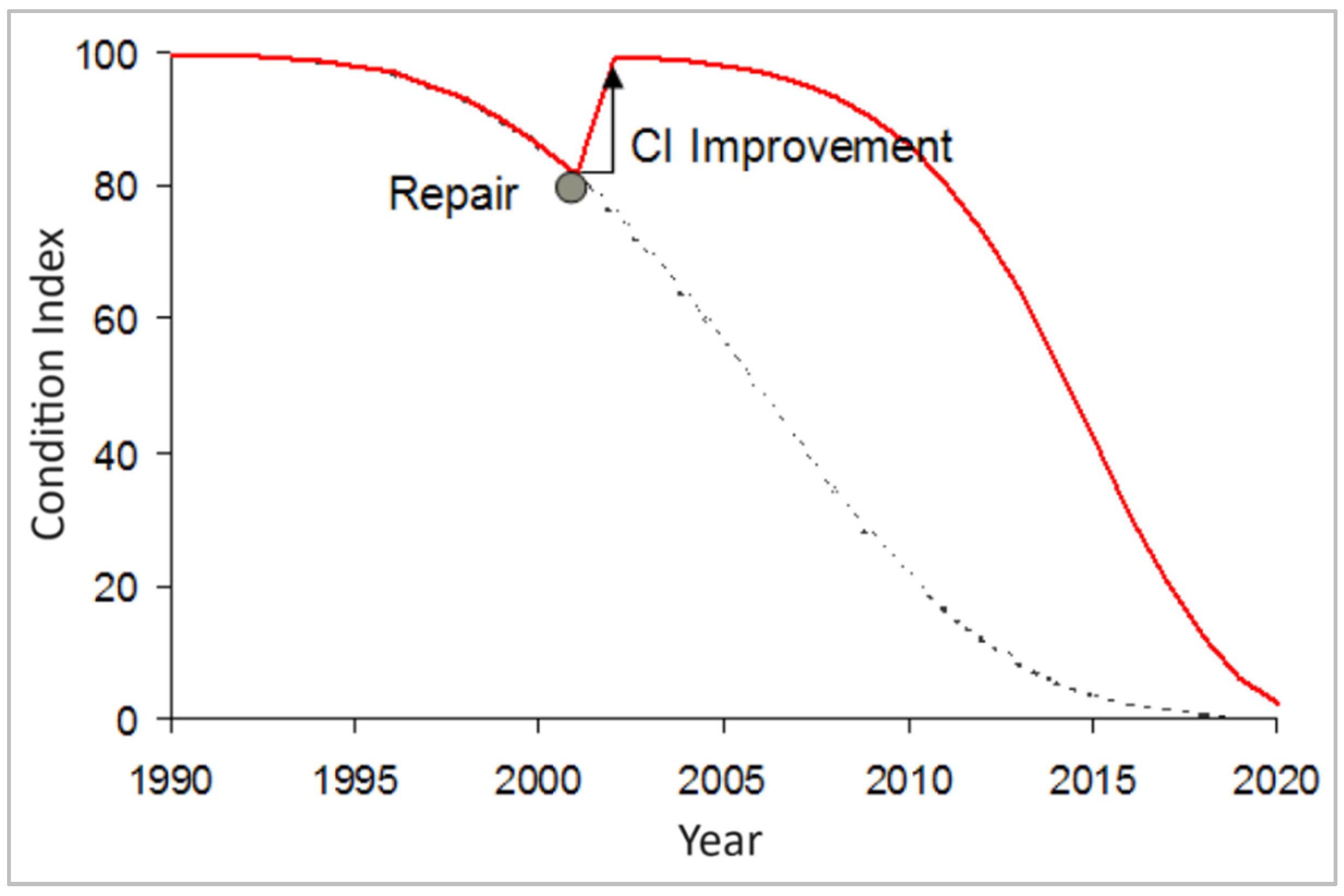
The condition index is a “value that is objective, repeatable, and clearly communicates the general physical health of the asset” [15]. Based on the current condition, a model showing how the CI degrades over time is then assumed for each infrastructure component (e.g., Figure 1). CI is a maximum of 100 at initial construction and approaches the minimum of 0 as it degrades nonlinearly, as indicated by the red line. Routine maintenance is assumed to be completed throughout the asset’s service life within the degradation model. When repairs are conducted, indicated by an upward jump in the asset’s condition, e.g., the CI improvement in Figure 1, the CI may increase at the next inspection. The red line after the repair deviates from the original trajectory of the dotted line and indicates a revised lifecycle condition trend with an extended service life. Likewise, if there is a major degradation event, CI may be lower than anticipated at the next inspection. The degradation model of an infrastructure component may be adjusted slightly based on the CI determined at subsequent inspections. Tracking the CI of an infrastructure component over time is helpful to those charged with prioritizing and financing repair and recapitalization projects. Currently, the degradation model for each component does not vary between types of HVAC components and does not vary with geographic location.

Figure 1.
Typical life cycle condition trend, including repair [11].
Environmental degradation of HVAC infrastructure can be direct or indirect. Direct degradation involves factors that come into physical contact with or physically influence the components. Examples of direct degradation from environmental factors include damage from strong winds or material corrosion from excessive rain. In contrast, indirect degradation causes the HVAC infrastructure to be used more often or in a different way, which, in turn, increases degradation. Examples of indirect degradation from environmental factors include increased run time in extremely hot or cold environments.
This study considered both direct and indirect degradation of HVAC sections across 49 Air Force and Space Force Bases within the USA. Other factors that may cause infrastructure degradation were not accounted for in this study. The research question of interest is, What are the environmental factors that cause the highest degradation rates to HVAC systems, and, do the relevant environmental factors change when looking at specific subsets of HVAC systems? Section 3 will summarize some relevant literature about infrastructure degradation this study built upon.
3. Literature Review
Insights into how HVAC systems degrade can be gleaned from investigating how the materials they are commonly made of degrade. In a study about how aluminum reacts in acidic and alkaline solutions, it was found that the most common source of degradation was from direct contact with alkaline solutions [16]. It was more difficult to predict the effects in acidic environments, as it depended on other factors such as concentration and temperature. Another study on the effect of relative humidity on an aluminum alloy found that even normal humidity can significantly embrittle it at room temperature [4]. A different study on the valorization of aluminum on the mechanical performance of mortar subjected to cycles of freeze–thaw found that the compressive strength of mortars with aluminum decreased significantly when exposed to freeze–thaw cycles compared with the control mortar without aluminum [5].
Another study investigated temperature and humidity and found that with temperature increases, the aging of silicone rubbers became more severe [6]. It also found that existing water molecules from humidified gases can accelerate the aging of the rubber. In steel, one study of steel–concrete composite girders found that the most critical temperature gradient occurs on sunny days when higher temperatures and radiation are prevalent [17]. Another study on the durability of steel joints under freeze–thaw conditions found that hot and wet environments controlled the lower bound of joint strength [7]. It also determined that steel joints immersed in saltwater (lower pH) decreased in strength significantly.
Within HVAC systems, ultraviolet light (UVC) used to kill microbes and maintain clean air flow has been shown to degrade surrounding materials due to poor shielding or improper layering of the HVAC system [18]. Further, photoaging, a process that can be initiated by UVC, air, and pollutants and enhanced by water, organic solvents, and temperature, can occur in polymers within HVAC components [19]. Because the UVC wavelength used for HVAC disinfection is also emitted by the sun, solar radiation may cause HVAC systems to degrade and lose performance efficiency.
There has been little research into environmental factors that cause degradation of HVAC components or systems. However, one preliminary study compared HVAC air handler units at four locations in the USA in different climate zones and concluded that temperature and humidity affected degradation rate [20]. Another compared HVAC components across 21 locations in the USA using three environmental and four non-environmental factors, wherein a machine learning model suggested temperature, component age and precipitation were the most relevant features to predict HVAC degradation rate [21]. In summary, the literature [12,13,14,15,16,17,18,19,20,21] shows that relative humidity, freeze–thaw cycles, pH, radiation, the presence of water, and temperature could be factors in HVAC infrastructure degradation.
4. Methods
4.1. HVAC Data
For this study, infrastructure inspection reports from 49 Air Force and Space Force bases in the USA were pulled from BUILDER between November and December 2022. The reports contain the date and CI for every inspection conducted on each section of infrastructure ever recorded in BUILDER, totaling data from over 2.4 million inspections. Data reduction and sorting were completed using Python computing tools in Google Colaboratory.
The BUILDER reports from each base were concatenated and filtered to keep only HVAC system data. Inspection reports for the same section were then grouped together. Next, data were arranged in sequential inspection pairs with an initial CI for the initial inspection date and a follow-on CI for the follow-on inspection date. Data for sections that had only been inspected once were removed since there was no follow-on inspection to determine the change in CI over time. Sections that were inspected twice had one inspection pair, sections that were inspected three times had two inspection pairs, and so on. Because this investigation focused on the causes of HVAC degradation, all cases in which the inspection score increased between the initial and follow-on inspections, e.g., due to infrastructure repair, were removed. Data in which the duration between inspections was less than 31 days were also removed to prevent outliers from potentially skewing the results.
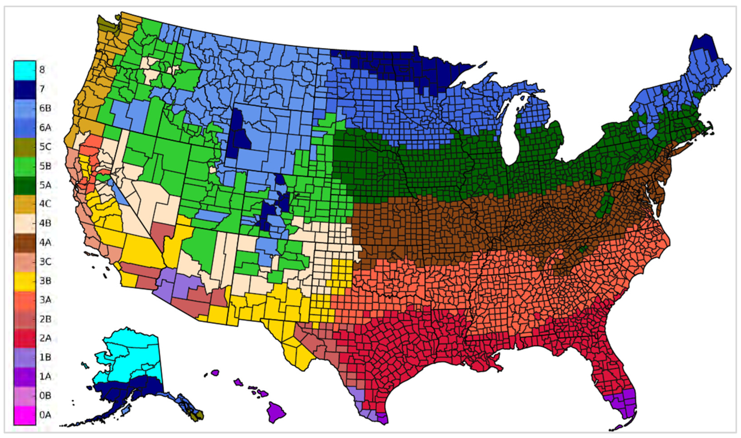
Base locations were further classified by climate zones as specified by the American Society of Heating, Refrigerating and Air-Conditioning Engineers (ASHRAE) [22]. The ASHRAE standard is a prominent reference for HVAC design professionals and a map of climate zones in the USA, as shown in Figure 2.

Figure 2.
Map of climate zones in the USA [22].
A summary of how the 49 bases in this study align within each climate zone is shown in Table 2. Of note, there are five climate zones that do not contain any bases in this study.
Table 2.
Summary of Air Force and Space Force bases by climate zone.
With HVAC section data arranged by inspection pairs, the duration of time between inspections and the change in condition index over time becomes apparent. Because inspections occur over different time intervals, a degradation rate metric, DR, was calculated and used to compare HVAC sections (Equation (1)).
where:
DR is the degradation rate;
CI2 is condition index of the follow-on inspection;
CI1 is condition index of the initial inspection;
t2 is date of the follow-on inspection;
t1 is date of the initial inspection.
DR is the metric this investigation focused on in pursuit of determining the environmental factors that cause the highest degradation rates to HVAC systems. The denominator of Equation (1) will always be a positive number of days. The numerator will be a unitless integer between −100 and 100; it will be negative if degradation occurred between the initial and follow-on inspections, will be zero if no change in condition index was observed between inspections, and will be positive if a repair occurred between inspections. The term “30” in Equation (1) converts days to months, approximately, and allows for the overall unit of DR being percentage points per month.
4.2. Environmental Data
In addition to HVAC condition data, environmental data were collected for this investigation based on the literature discussed in Section 3. Metrics included precipitation (mm), minimum and maximum relative humidity (%), minimum and maximum temperature (°K), mean daily windspeed (m/s), surface shortwave radiation (W/m2), and atmospheric deposition of free acidity (H+) as pH were collected [23]. Each metric was recorded daily at approximately 40–420 locations across the USA over the data range of the HVAC inspection data and downscaled to a 1 km2 grid. These point data were interpolated using the inverse-distance weighting technique [24], which estimates the values of the metric in unknown locations with each point’s value weighing more in the estimation with proximity. Data preprocessing was conducted in ArcGIS Pro version 3.2 and R version 3.1.
An additional metric of freeze–thaw boundary crossings was derived from the collected environmental data. If, within a given day, the minimum temperature was below freezing and the maximum temperature was above, it would be recorded as one boundary crossing. While additional environmental factors may impact HVAC infrastructure degradation rate, the factors listed in this section were expected to have an impact due to previous research described in Section 3 and engineering judgment.
4.3. Data Assembly and Analysis
HVAC data from BUILDER was paired with the environmental data that each section was exposed to between inspections. Data for each environmental feature for every third day between the initial and follow-up inspections were extracted and associated with each HVAC section’s DR. Note, because environmental data from every third day was appended to the HVAC data, some extreme values may not have been captured. Further, precipitation and freeze–thaw boundary crossing data can be interpreted in relative, but not absolute terms.
In addition to the environmental data discussed in Section 4.2, it was acknowledged that infrastructure age may play a role in degradation. Lacking other information, it seems reasonable to expect older infrastructure sections to degrade at a higher rate due to wear and tear from normal use or degradation at the material level. From the infrastructure operator’s perspective, it may be more difficult to obtain replacement parts for older infrastructure sections, and there may be a bias to replace older sections before newer ones. Therefore, section install date was included in this study as a feature when modeling factors affecting degradation rate. The list of features used in this study is shown in Table 3.
Table 3.
Environmental features used in this study.
The final dataset used during the analysis phase of this study contained 69,376 inspection pairs. The average CI of the initial inspection was 87.1, with a standard deviation of 12.3, and the average decrease in CI between inspections was 9.35, with a standard deviation of 14.8. The average duration of time between inspections was 1322 days (~3 years and 7.5 months), with a standard deviation of 738 days (~2 years).
Data were examined, and the results are reported in Section 5 in multiple forms. Initially, all HVAC sections in the total dataset are reported and discussed in aggregate and by ASHRAE climate zone. By analyzing the climate zones that include HVAC sections with the highest (or lowest) degradation rates, along with the values of environmental features to which they were exposed, the environmental factors that lead to greater (or lower) rates of degradation can be uncovered.
The data were broken down in three distinct ways to uncover additional, nuanced insights into which environmental features are most critical to predicting HVAC section degradation rates. First, results are presented by component type per the seven unique types listed in Section 2. As each HVAC component type performs different functions, may be made of different materials and may be physically located in different sites within or outside a facility, it follows that they may degrade at different rates.
Second, data were divided into three subgroups based on the CI at the time of the initial inspection. Per Table 1, the three subgroups were red, amber, and green HVAC infrastructure sections. Amber sections were expected to have a fairly consistent average DR amongst the data because the slope of the condition index trend in Figure 1 is fairly uniform between CI = 40 to CI = 69. Because the majority of the DAF infrastructure inventory was in the green subgroup, the green section data were investigated separately. Both green and red sections were expected to have a lower absolute value of DR than amber sections due to the condition index trend in Figure 1. Investigating results from red sections separately from the total may provide insights into the degradation of DAF’s assets in the worst condition.
The third means to analyze data and report results was in three subgroups by DR. While the majority of HVAC sections in this study had modest DR values, some outliers had comparatively high magnitude DRs. The low DR subgroup contained data within the mean ± 1 standard deviation. The medium DR subgroup contained data with values of DR that deviated from the mean by between −1 and −2 standard deviations. Lastly, the high DR subgroup contained data with values of DR that exceeded the mean by −2 standard deviations or more. While DR would not be known by HVAC system operators a priori with assurance, analysis of these three DR subgroups may provide insight into unique environmental factors that may influence higher or lower DRs.
4.4. Modeling Approach
The environmental factors that impact HVAC degradation are discoverable when measurements of those features contribute to creating predictive models for the degradation rate. Moreover, the contribution of each feature to the model’s predictive power indicates a stronger relationship between the environmental factor and degradation.
Random forests (RFs) are predictive models that have remarkable performance with few tuning parameters and can be used for both prediction and parameter value estimation [25]. RF is a nonparametric modeling method. Such modeling methods do not limit the relationships between features and the predicted variable [26] as parametric models like linear regression do. They have successfully been used in environmental science and engineering contexts, handling outliers well without overfitting [27]. The approach employed in much of the analysis of the final dataset was to determine relative feature importance for RF models trained to predict DR. The importance of features to predictive models provides insights into the relationships between environmental measurements and the DR.
The RF analysis was completed using the Scikit-Learn library [28]. The Gini importance (GI) estimates each feature’s contribution to a predictive model. An RF is made from many decision trees. While each decision tree is constructed, the fitting algorithm selects a feature and a value for that feature about which to split the data. The algorithm compares the mean squared error (MSE) of the model both before and after the split. The reduction in MSE is then attributed to the respective feature. The aggregate reduction in MSE constitutes the GI for each feature, which is normalized for each tree and averaged across all trees in the forest to determine the GI [26,28]. The GI cannot be used to infer a positive or inverse relationship, however. For a given model, the GI for each feature represents the portion of the total mean squared error that was reduced by it. The GI values for all features sum to one, accounting for the total explanatory power of the model.
GI provides more insight when a model has better predictive power. To estimate the predictive power of the modeling technique, K-fold cross-validation was applied. K-fold cross-validation creates several models from the data. In this study, the dataset was split into k = 5 shuffled independent subsets. Each model was trained on four (k − 1) portions of the data. The accuracy of each model was estimated on the data withheld from the model training process. This was repeated using each of the subsets as a validation set once. The final estimation of performance reported was the average of the models. Root mean square error (RMSE) gives a good estimate of the performance of the modeling technique (Equation (2)), and is reported for each model described in Section 5. All modeling was performed in the Python programming language using the open source Jupyter Notebook software version 6.4.5.
where:
RMSE is the root mean square error;
n is the number of observations;
yi is the actual value for the ith observation;
ŷi is the predicted value for the ith observation.
5. Results and Discussion
5.1. Comparison of Degradation Rates
Table 4 shows the average DR, standard deviation of DR, and number of datapoints for the total dataset as well as the various subgroups discussed in Section 4.3. Cells are shaded when the average DR of a subgroup showed a statistically significant difference (higher in red, lower in green) from the average DR of the total dataset from a two-tailed t-test of the means (p < 0.05).
Table 4.
Degradation rate of various datasets *.
Across the total dataset, the average DR was −0.389 percentage points per month. Energy supply, heat, and cooling sections had a significantly different DR than that of the total dataset; energy supply and heat sections degraded at a slower rate, while cooling degraded more rapidly than the average across all HVAC sections. This finding is significant to facility use, as cooling requirements are vital to keeping computers, servers, and other sensitive equipment effectively.
Because the amber sections were expected to have a more consistent DR than the other subgroups per the life cycle condition trend (Figure 1), the amber sections were expected to have a small standard deviation. However, the standard deviation of the amber sections was larger than that of the red sections. This finding could be due to repairs altering the slope of the life cycle condition trend such that degradation of the amber sections was not as predictable as expected. Owing to the shallower slope of the life cycle condition trend (Figure 1), the average DR of both the green and red sections had a lower absolute value than the amber sections.
5.2. Individual Environmental Feature Impacts on Degradation Rate
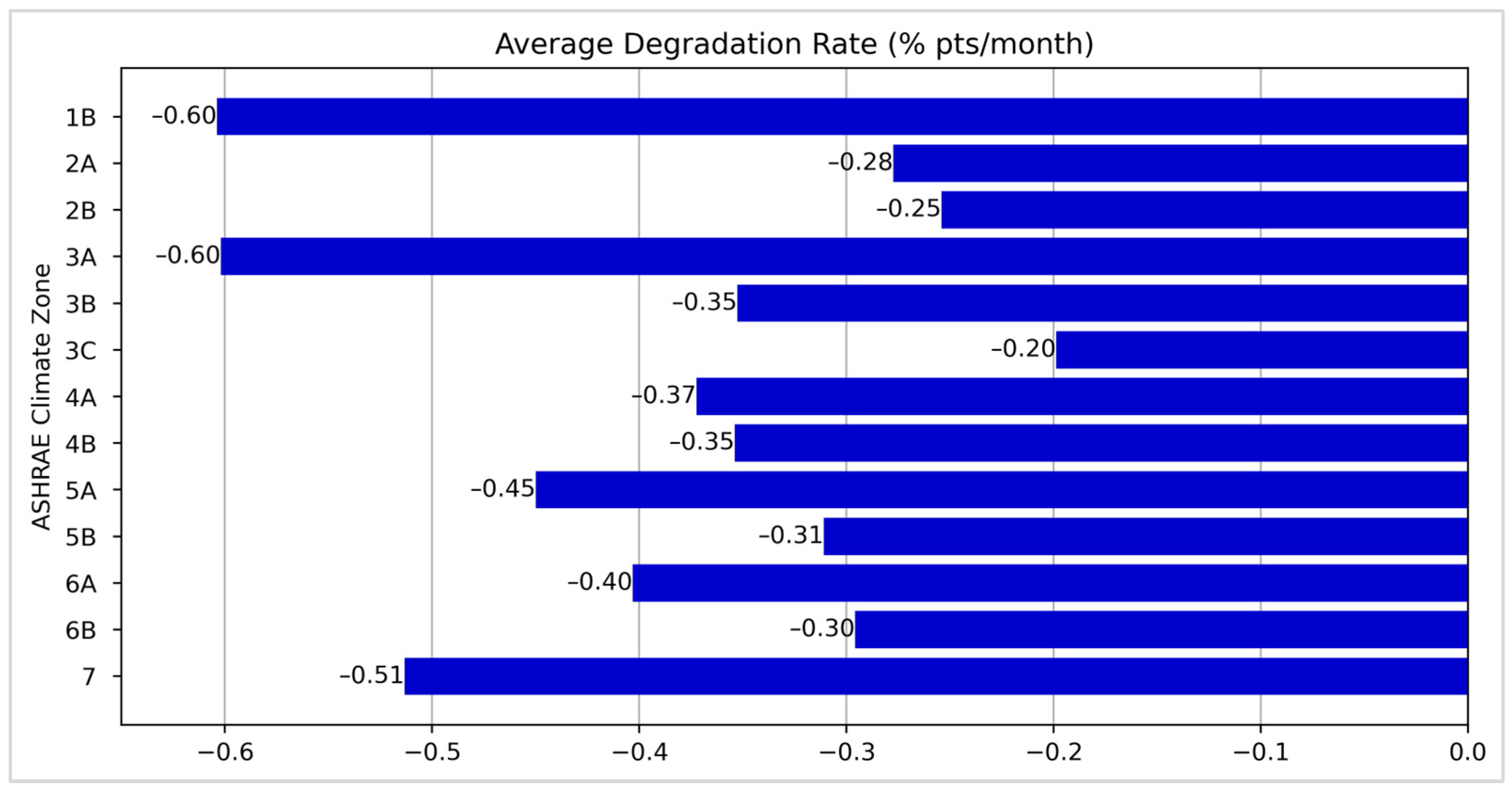
Evaluating the average degradation rate for each climate zone highlighted a few major trends. Figure 3 shows the average DR for all HVAC sections by climate zone. Of the 13 climate zones, 8 were considered outliers, where the average DR was more than 0.1 percentage point per month different than the average DR for the total dataset (−0.389% pts/mo). The average DR in four outlier zones was more than 0.1 percentage point per month greater, and the average DR in the other four outlier zones was more than 0.1 percentage point per month less than the average DR.
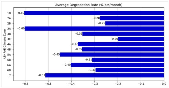
Figure 3.
Average degradation rate by climate zone.
HVAC sections in climate zones 1B, 3A, and 7 were outliers that had a substantially higher average DR than sections in other climate zones. Zones 1B and 7 tended to have fairly extreme environmental factors. Zone 1B is in the southwest USA (Figure 2) and is extremely hot and dry, while zone 7 is in the northern USA and is very cold and prone to arctic storm systems in the winter. Both zones 1B and 7 require a significant amount of heating or cooling, respectively, to maintain occupant comfort and condition air for mission-critical equipment. HVAC sections in zone 3C had the lowest DR of any region in the USA (Figure 3). Zone 3C is coastal and temperate, which should lead to a lower operational usage of HVAC systems.
Degradation rates for HVAC sections in the eight outlier climate zones were further evaluated by the 10 environmental features used in this study to identify any trends (Table 5). Cells are shaded where the average value for a given feature in at least three of the four climate regions in an outlier group either exceeded (red) or was less than (green) the feature average for the total dataset. There were no cases where the majority of lower DR outliers had, for example, a lower average feature value than the total dataset, while the majority of the higher DR outliers had a higher feature value for the same feature.
Table 5.
Feature values by climate zone *.
There are some valuable observations to note between climate zones, however. The average value of both minimum and maximum relative humidity in three of the four higher DR outlier climate zones exceeded that of the total dataset, indicating that higher humidity correlated with higher HVAC section degradation rates. Higher humidity can cause an increase in operational usage of HVAC systems in humid environments, which could have led to indirect degradation, and is supported by [4,6,20]. This finding may be useful to those maintaining and allocating resources toward geographically distributed infrastructure portfolios.
Lower maximum temperatures, less precipitation, and fewer freeze–thaw boundary crossings were characteristics of HVAC sections in three of the four lower DR outlier climate zones. Additionally, three of four lower DR outlier climate zones had higher minimum temperatures, indicating that more moderate climate zones with less extreme temperatures correlate to a lower DR. Average radiation was higher in the lower DR outlier climate zones than the average radiation to which the total dataset was exposed; this contrasts with expectations based on UVC exposure in HVAC systems per [18]. Average wind speed was higher than that of the total dataset in three of four climate zones in both the lower and higher outlier climate zone groups. Finally, the average section install date in three of four higher DR outlier climate zones was older than the average of the total dataset, indicating older HVAC sections may be prone to higher DRs.
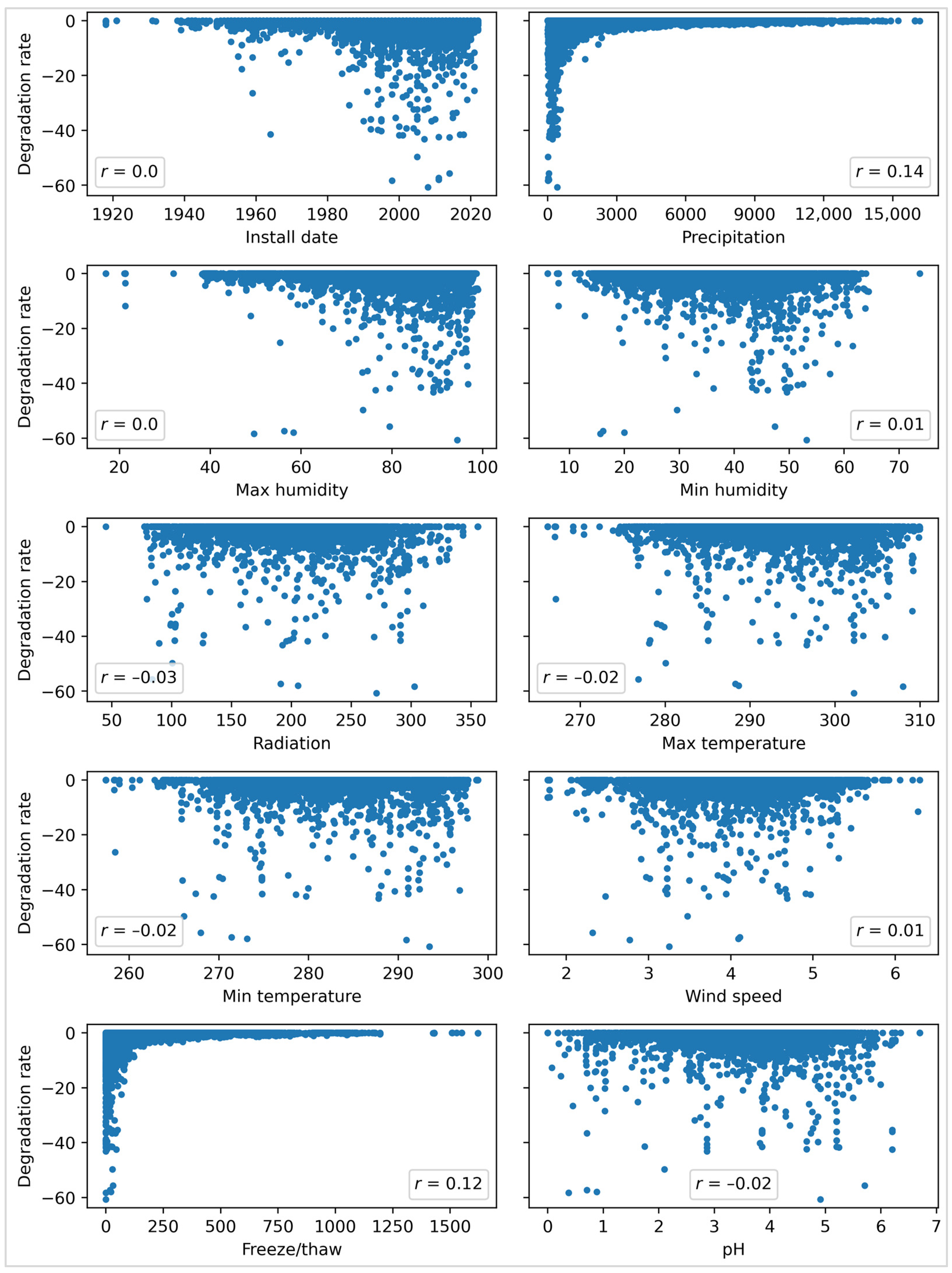
Figure 4 shows scatter plots representing how each of the 10 features correlated to the DR for the total dataset. The two most correlated features to DR were precipitation (Pearson correlation coefficient, r = 0.14) and freeze–thaw (r = 0.12), yet their correlation coefficients were still fairly modest. Precipitation and freeze–thaw were environmental factors expected to lead to higher degradation rates [7]. Correlation coefficients for the other eight features ranged from −0.03 to 0.01.

Figure 4.
Correlations between average degradation rate and each feature.
The scatter plots can also provide insight into the observations across the feature space of each feature. Values of install date, maximum humidity, and maximum temperature were more heavily skewed toward the higher end of their relative feature space. The models are not likely to robustly relate other factors to degradation rate when there are few samples. For example, sections installed before 1940 are few but all showed a low DR; the RF model described in Section 5.3 is capable of representing this relationship.
In contrast, radiation, wind speed, and pH are features with a fairly balanced number of observations across their respective feature spaces. This may cause the model training algorithm to select features based on more dynamic relationships between features.
5.3. Random Forest Results of Environmental Feature Impact on Degradation Rate
5.3.1. Total Dataset
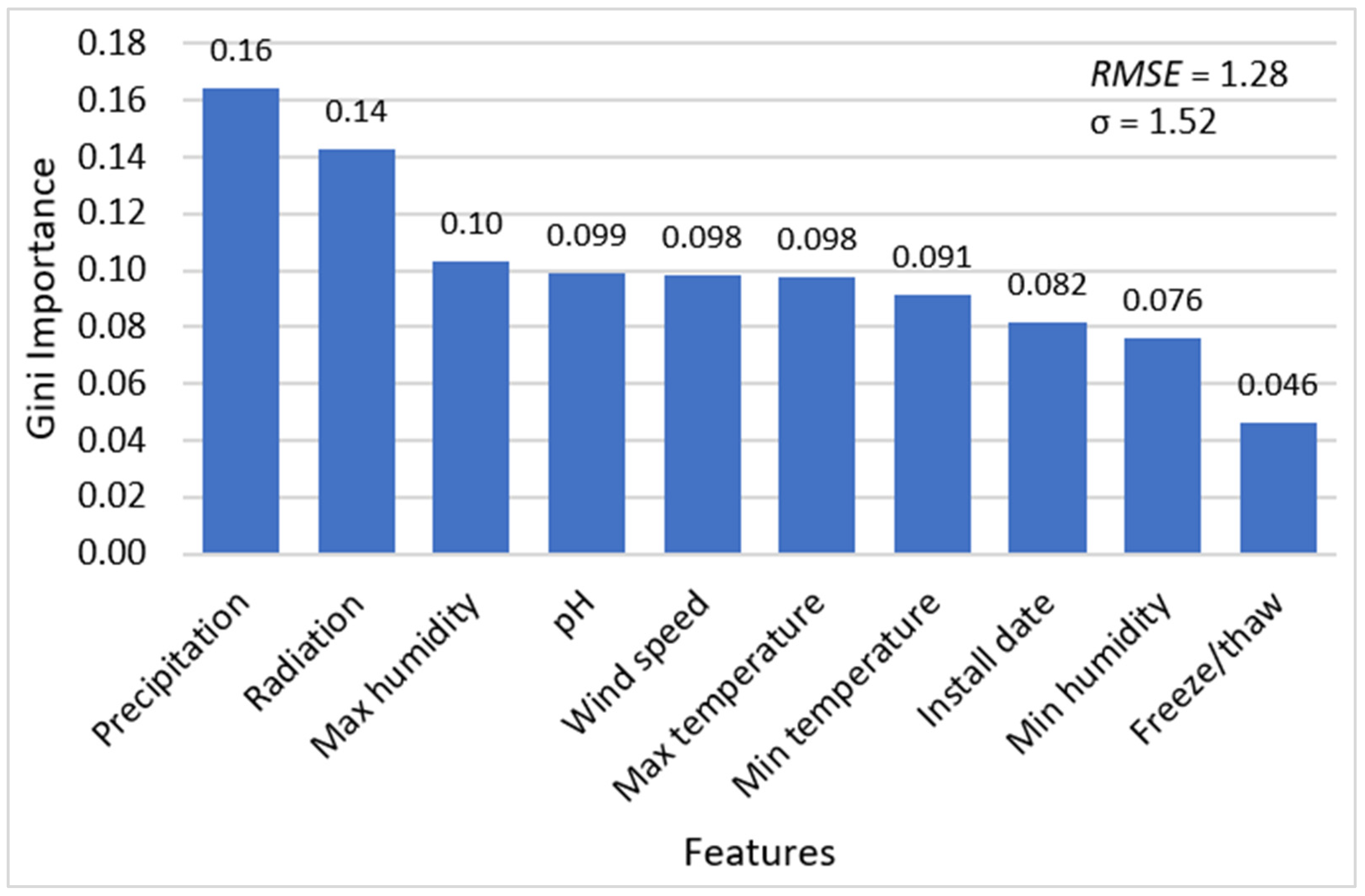
Using the total dataset, Figure 5 shows all 10 features on the x-axis and the GI of each on the y-axis. The RMSE in the RF model was 1.28 percentage points per month. The standard deviation, σ, of the total dataset was 1.52 percentage points per month; this indicates the model is better at predicting DR for a given HVAC section than by simply assuming the mean value and demonstrates credence to the GI values.

Figure 5.
Feature importance of the total dataset.
Based on the model for the total dataset, precipitation and radiation had a GI well above the other features and, thus, are the most important features in predicting the DR. The GI of the next four features (maximum humidity, pH, wind speed, and maximum temperature) were fairly constant. The GIs of minimum temperature, install date, and minimum humidity were less than that of the previous four, and freeze–thaw was distinctly the least important feature when predicting DR in the total dataset. The data showed that age is not as important as environmental features in predicting DR for all HVAC sections in aggregate.
From investigating the correlations between individual features and DR in Section 5.2, it was expected that precipitation might be relevant in the RF model. Physically, precipitation causes a direct impact on infrastructure as water comes into contact with sections exposed to the elements and may cause corrosion in ferrous metals over time. The words “rust” or “corrosion” were mentioned in 9.1% of all the inspection comments across the BUILDER reports, which supports the RF model’s output as precipitation being the most important feature in predicting degradation rate.
It was also expected that freeze–thaw would be important. However, as discussed in Section 4.2, freeze–thaw boundary crossings is a derived feature from the minimum and maximum daily temperatures. It follows that since minimum and maximum temperatures are included as separate features in the RF model, the addition of freeze–thaw boundary crossings was of little importance in reducing the RMSE of the model predictions, resulting in the lowest GI among all the features.
It was not expected that shortwave radiation would also have a relatively high GI. Radiation and precipitation were not well correlated (r = 0.0239), and environmentally, cloud cover both blocks solar radiation and can facilitate precipitation. UV radiation has been shown to cause direct deterioration to HVAC systems [18], but radiation is correlated to high temperatures (r = 0.807) and can also induce indirect deterioration from longer HVAC system run times.
5.3.2. Component Type Subgroups
Separate RF models were created using subgroups of the dataset corresponding to each component type. Table 6 shows the GI of each feature for each subgroup. For reference, the GI values for the total dataset are also shown. The GI of features in a subgroup’s analysis that were more than 0.05 above that of the total dataset are highlighted in red; the GI of features in a subgroup’s analysis that were less than that of the total dataset by 0.05 or more are highlighted in green.
Table 6.
Feature importance by component type subgroups *.
RMSEs were lower than standard deviations for all models, indicating all the RF models had better predictive power than simply selecting the mean value of DR for the subgroup. The distribution and terminal and package unit subgroups were the only two of the seven subgroups where the GI for all features were within ±0.05 of the GI of the corresponding feature in the total dataset. This is not surprising since these two subgroups have the largest number of datapoints and, thus, are less prone to outliers.
Within the energy supply sections, maximum humidity was particularly important in predicting degradation rate, with a GI of 0.26 (Table 6); additionally, the average maximum relative humidity to which the energy supply sections were exposed was 4.8% higher than the total dataset. It was expected that the DR of the heating sections may be impacted a great deal by minimum temperature, where run times and indirect degradation of heating systems would increase in colder climates, but this was not a finding from the analysis. Rather, radiation was particularly important in the RF model predicting heating section DR; while the average radiation to which heating sections were exposed was the same as the average radiation for the total dataset, radiation had a GI of 0.20 in the heating sections model.
On the contrary, radiation (GI = 0.073) was particularly unimportant in the RF model predicting the DR of the cooling sections, while pH was the environmental feature with the highest GI (0.22). pH was expected to be related to degradation [7], was deemed much more important to controls sections than the total dataset, and had the largest GI (0.16) in the controls subgroup.
The GIs of 7 of the 10 features differed by more than 0.05 in the RF model of other sections when compared with the total dataset. The other subgroup has the fewest datapoints, which could have contributed to the vastly different GIs.
5.3.3. Initial Condition Index Subgroups
Separate RF models were created using subsets of the data corresponding to the initial condition index: either green, amber, or red. Table 7 shows the GI of each feature for each subgroup along with the GIs for the total dataset for reference. The GI of features in a subgroup’s analysis that were more than 0.05 above that of the total dataset are highlighted in red; feature weights that were less than 0.05 below are highlighted in green. The RMSE for the model of each subgroup was smaller than the standard deviation, indicating reasonable model performance.
Table 7.
Feature importance by initial condition index subgroups *.
The green subgroup contained the most datapoints (95%) of any initial CI subgroup; therefore, as expected, the GI for each feature in the green dataset was fairly consistent with that of the total dataset.
In the amber subgroup, precipitation was the most important feature, but its GI was 0.22, meaning the RF model of the amber sections relied on precipitation much more to predict DR than the RF model for the total dataset. Despite average total precipitation between inspection pairs of amber sections being 5.1% lower than the average across the total dataset, cumulative direct environmental effects from precipitation could have led to its recognition as an important feature. Minimum humidity was among the least important feature for the total dataset; however, it was very important to the amber subgroup’s RF model. GIs for minimum and maximum humidity of the amber sections were both 0.15, while the average values of minimum and maximum humidity to which the amber sections were exposed were modestly higher (1.8% and 1.2%, respectively) than the total dataset. These results could indicate indirect degradation from potentially high run times of the amber sections due to the increased humidity. Section install date was particularly unimportant within the amber subgroup, with a GI of only 0.029, despite the average age of amber sections being about seven years older than the average in the total dataset.
Within the red subgroup, the average age was 10 years older than that of the total dataset, indicating that older age may be associated with a lower initial CI. Precipitation was again very important in the RF model’s predictive power (GI = 0.23), while average total precipitation was 9.0% higher in the red subgroup than the total dataset. Maximum humidity (GI = 0.29) and pH (GI = 0.19) also had significantly higher GIs for the red sections than in the total dataset. Maximum humidity averaged 3.4% more and pH averaged 1.5% less in the red sections than the total dataset. The GI of the top three features in the red subgroup’s model summed to 0.71, meaning they can explain over two-thirds of the variance in the RF model. This finding could simplify the prediction of DR for HVAC infrastructure in the red zone by monitoring just precipitation, maximum humidity, and pH.
5.3.4. Degradation Rate Subgroups
The GIs for the 10 features in the three DR subgroups are shown in Table 8 along with the GIs for the total dataset for reference. Feature weights for a subgroup’s analysis that were more than 0.05 above that of the total dataset are highlighted in red; feature weights that were at least 0.05 less than that of the total dataset are highlighted in green. The RMSE for the model of each subgroup was smaller than the standard deviation of the subgroup, indicating reasonable model performance.
Table 8.
Feature importance by degradation rate subgroups *.
The low DR subgroup contained 79% of datapoints; thus, the GI of its features were expected to mimic those of the total dataset. However, the two most important features in the total dataset, precipitation (GI = 0.086) and radiation (GI = 0.089), were much less important to the low DR model. The most important feature of the low DR model was install date, with a GI of 0.17, despite the average section age being about the same as that of the total dataset.
Install date was again fairly important to the medium DR subgroup (GI = 0.14), whose sections were, on average, 1 year older than the average age across the total dataset. Within the high DR subgroup, the RF model indicated that precipitation was the most important feature (GI = 0.27), and much more important than in the total dataset (GI = 0.16). High DR sections, on average, had a shorter duration of time between inspection pairs, but the average precipitation per month that sections were exposed to was 9.2% less than the total dataset. Additionally, minimum humidity was much more important for high DR sections (GI = 0.14) than to the total dataset (GI = 0.076), while minimum humidity values were 3.3% lower in the high DR subgroup. These findings indicate that when an HVAC section degrades rapidly, precipitation and minimum humidity are the best environmental indicators. However, because the higher DR subgroup experienced lower precipitation and minimum humidity than the total dataset, the results seem to be in conflict with previous claims that higher precipitation and higher humidity seem to be associated with a greater DR. The sample size of the high DR subgroup was fairly small (3.3% of the total dataset), which could have skewed results.
6. Conclusions
This study explored how environmental factors impacted the degradation rates of HVAC systems at 49 Air Force and Space Force bases across the USA. Over 69,000 pairs of HVAC section inspection data were compiled. Nine environmental features were investigated: precipitation, minimum humidity, maximum humidity, minimum temperature, maximum temperature, wind speed, radiation, pH, and freeze–thaw. Installation date, or age, was another feature explored. Random forest models were constructed to determine the relative importance of each feature when predicting degradation rate.
By ASHRAE climate zone, several findings about the HVAC degradation rate were discovered.
- Decreased precipitation, fewer freeze–thaw cycles, and a more moderate climate with higher minimum temperatures and lower maximum temperatures led to lower rates of HVAC infrastructure degradation;
- Higher relative humidity led to higher rates of HVAC infrastructure degradation.
Additional observations were made about the relative importance of environmental features for predicting the degradation rate across the total HVAC dataset.
- Considering environmental features individually, total precipitation and freeze–thaw boundary crossings were the most correlated to degradation rate across the total HVAC dataset;
- Using a random forest model, the most critical features in predicting degradation rate were precipitation and radiation. The age of the infrastructure section was not a highly weighted feature.
Precipitation and maximum relative humidity were frequently determined as important environmental features in random forest models specific to a component type of HVAC infrastructure, though feature importance varied between component types.
- In energy supply sections, maximum humidity was particularly important, followed by radiation and precipitation;
- In heating sections, radiation was the most important feature, followed by precipitation and wind speed;
- In cooling sections, pH was most important, followed by precipitation, then maximum humidity. Radiation was not an important feature when predicting the cooling system degradation rate;
- In controls sections, pH was particularly important, followed by radiation, then precipitation and maximum humidity.
Understanding how individual environmental factors relate to infrastructure degradation can be useful to asset managers and decision makers. Accurate predictions of degradation rates are key information when making trade-offs between various repair actions and determining maintenance schedules. Ultimately, a better understanding of how infrastructure degrades could inform how society reshapes infrastructure for a more sustainable and resilient future.
Despite the various findings presented herein, there are several limitations of this study. The environmental data associated with each HVAC section only included those effects that occurred between inspection pairs. Therefore, cumulative effects across the lifetime of the HVAC infrastructure were not captured nor considered by the models. The HVAC inspection data from BUILDER was created by individual inspectors and were subjective. Therefore, inaccurate data could have affected the results. Other factors that may cause HVAC degradation were not considered, nor is their contribution to overall infrastructure degradation well known.
7. Next Steps
Future work could include predictive modeling of infrastructure degradation. This study can also be expanded geographically to increase the feature space of the environmental variables, and additional environmental features can be added to the dataset. The methodology described in this study can be applied to other infrastructure types, such as electrical or structural systems.
Author Contributions
Conceptualization, T.F. and J.W.; Methodology, T.F., J.W. and M.C. (Marcus Catchpole); Validation, M.C. (Marcus Catchpole); Formal analysis, T.F.; Investigation, T.F., M.C. (Michelle Cabonce) and S.B.; Resources, S.B.; Data curation, T.F., J.A. and J.W.; Writing—original draft, T.F., J.A., J.W., M.C. (Marcus Catchpole), M.C. (Michelle Cabonce) and S.B.; Writing—review & editing, T.F., J.A., J.W., M.C. (Marcus Catchpole), M.C. (Michelle Cabonce) and S.B.; Visualization, M.C. (Marcus Catchpole); Supervision, T.F. and J.A.; Project administration, T.F. and J.W. All authors have read and agreed to the published version of the manuscript.
Funding
This research received no external funding.
Institutional Review Board Statement
Not applicable.
Informed Consent Statement
Not applicable.
Data Availability Statement
The data presented in this study are available on request from the corresponding author.
Acknowledgments
The authors thank Daniel Noonan, who derived the freeze–thaw feature.
Conflicts of Interest
The authors declare no conflicts of interest. The views expressed in this paper are those of the authors and not necessarily reflect those of the United States Air Force Academy, the Air Force, the Department of Defense, or the U.S. Government.
References
- Statistica. Total New Infrastructure Construction in the U.S. 2012–2022, by Segment. Available online: https://www.statista.com/statistics/1307529/total-new-infrastructure-construction-in-the-usa-by-segment/ (accessed on 6 November 2023).
- Architecture 2030. Why the Built Environment? Available online: https://www.architecture2030.org/why-the-built-environment/#:~:text=The%20built%20environment%20is%20responsible,of%20annual%20global%20CO2%20emissions (accessed on 6 November 2023).
- Okafor, J. Environmental Impact of Construction and the Built Environment. Available online: https://www.trvst.world/environment/environmental-impact-of-construction-and-the-built-environment/ (accessed on 6 November 2023).
- Safyari, M.; Hojo, T.; Moshtaghi, M. Effect of environmental relative humidity on hydrogen-induced mechanical degradation in an al–zn–mg–cu alloy. Vacuum 2021, 192, 110489. [Google Scholar] [CrossRef]
- Tebbal, N.; Rahmouni, Z.E. Valorization of aluminum waste on the mechanical performance of mortar subjected to cycles of freeze-thaw. Procedia Comput. Sci. 2019, 158, 1114–1121. [Google Scholar] [CrossRef]
- Chang, H.; Wan, Z.; Chen, X.; Wan, J.; Luo, L.; Zhang, H.; Shu, S.; Tu, Z. Temperature and humidity effect on aging of silicone rubbers as sealing materials for proton exchange membrane fuel cell applications. Appl. Therm. Eng. 2016, 104, 472–478. [Google Scholar] [CrossRef]
- Heshmati, M.; Haghani, R.; Al-Emrani, M. Durability of bonded FRP-to-steel joints: Effects of moisture, de-icing salt solution, temperature and FRP type. Compos. Part B Eng. 2017, 119, 153–167. [Google Scholar] [CrossRef]
- ASCE. Infrastructure Investment Gap 2020–2029. Available online: https://infrastructurereportcard.org/resources/investment-gap-2020-2029/ (accessed on 6 November 2023).
- USGS. What Are Some of the Signs of Climate Change? Available online: https://www.usgs.gov/faqs/what-are-some-signs-climate-change (accessed on 6 November 2023).
- USEPA. Climate Change Impacts on the Built Environment. Available online: https://www.epa.gov/climateimpacts/climate-change-impacts-built-environment (accessed on 6 November 2023).
- Sloan, J.A.; Stanford, M.S.; Phelan, T.J.; Pocock, J.B. Infrastructure Truths for Air, Space, and Cyberspace. Air Space Power J. 2021, 35, 19–36. [Google Scholar]
- USECDEF. Standardizing Facility Condition Assessments. Available online: https://www.acq.osd.mil/eie/Downloads/FIM/DoD%20Facility%20Inspection%20Policy.pdf (accessed on 1 May 2023).
- USACE. BUILDER Inventory Guide V3.6.4. 30 March 2022. Available online: https://support.sms.erdc.dren.mil/downloads/files/builder-inventory-guide-3-6-4 (accessed on 8 January 2023).
- USACE. BUILDER Condition Assessment Guide V3.5.4. 6 February 2020. Available online: https://support.sms.erdc.dren.mil/focus-win/downloads/files/builder-condition-assessment-guide-3-5-4 (accessed on 8 January 2023).
- Grussing, M.N. Facility Degradation and Prediction Models for Sustainment, Restoration, and Modernization (SRM) Planning. USACE ERDC/CERL TR 12-13. Available online: https://apps.dtic.mil/sti/citations/ADA570002 (accessed on 8 January 2023).
- Boukerche, I.; Djerad, S.; Benmansour, L.; Tifouti, L.; Saleh, K. Degradability of aluminum in acidic and alkaline solutions. Corros. Sci. 2014, 78, 343–352. [Google Scholar] [CrossRef]
- Zhang, P.J.; Wang, C.S.; Wu, G.S.; Wang, Y. Temperature gradient models of steel-concrete composite girder based on long-term monitoring data. J. Constr. Steel Res. 2022, 194, 107309. [Google Scholar] [CrossRef]
- Kauffman, R.E. Study of the Degradation of Typical HVAC Materials, Filters and Components Irradiated by UVC Energy--Part I: Literature Search. ASHRAE Trans. 2012, 118, 638–648. [Google Scholar]
- Rabek, J.F. Polymer Photodegradation: Mechanisms and Experimental Methods, 1st ed.; Springer: Dordrecht, The Netherlands, 1995; pp. 1–664. [Google Scholar]
- Lamm, K.L.; Fortney, E.; Brown, S. Final Project: Investigation of Trends in Roof, HVAC, and Airfield Pavement Systems Using Localized Climate Data; Air Force Institute of Technology: Wright-Patterson AFB, OH, USA, 2019. [Google Scholar]
- Frank, T.E.; Aldred, J.R.; Boulware, S.B.; Cabonce, M.K.; White, J.H. Degradation of Heating, Ventilation, and Air Conditioning Components across Locations. Int. J. Struct. Const. Eng. 2023, 17, 437–442. [Google Scholar]
- Addendum to ANSI/ASHRAE Standard 169-2020; Climatic Data for Building Design Standards. ASHRAE: Peachtree Corners, GA, USA, 2021.
- NADP. National Trends Network. Wisconsin State Laboratory of Hygiene, Madison, WI, USA. Available online: https://nadp.slh.wisc.edu/networks/national-trends-network/ (accessed on 31 May 2023).
- Watson, D.F.; Philip, G.M. A Refinement of Inverse Distance Weighted Interpolation. Geoprocessing 1985, 2, 315–327. [Google Scholar]
- Probst, P.; Wright, M.N.; Boulesteix, A.-L. Hyperparameters and tuning strategies for random forest. Wiley Interdiscip. Rev. Data Min. Knowl. Discov. 2019, 9, e1301. [Google Scholar] [CrossRef]
- James, G.; Witten, D.; Hastie, T.; Tibshirani, R. An Introduction to Statistical Learning; Springer: New York, NY, USA, 2013. [Google Scholar]
- Gupta, S.; Aga, D.; Pruden, A.; Zhang, L.; Vikesland, P. Data analytics for environmental science and engineering research. Environ. Sci. Technol. 2012, 55, 10895–10907. [Google Scholar] [CrossRef] [PubMed]
- Pedregosa, F.; Varoquaux, G.; Gramfort, A.; Michel, V.; Thirion, B.; Grisel, O.; Blondel, M.; Prettenhofer, P.; Weiss, R.; Dubourg, V.; et al. Scikit-Learn: Machine Learning in Python. J. Mach. Learn. Res. 2011, 12, 2825–2830. [Google Scholar]
Disclaimer/Publisher’s Note: The statements, opinions and data contained in all publications are solely those of the individual author(s) and contributor(s) and not of MDPI and/or the editor(s). MDPI and/or the editor(s) disclaim responsibility for any injury to people or property resulting from any ideas, methods, instructions or products referred to in the content. |
© 2024 by the authors. Licensee MDPI, Basel, Switzerland. This article is an open access article distributed under the terms and conditions of the Creative Commons Attribution (CC BY) license (https://creativecommons.org/licenses/by/4.0/).