Abstract
Buildings remain pivotal in global energy consumption, necessitating a focused approach toward enhancing their energy efficiency to alleviate environmental impacts. Precise energy prediction stands as a linchpin in optimizing efficiency, offering indispensable foresight into future energy demands critical for sustainable environments. However, accurately forecasting energy consumption for individual households and commercial buildings presents multifaceted challenges due to their diverse consumption patterns. Leveraging the emerging landscape of the Internet of Things (IoT) in smart homes, coupled with AI-driven energy solutions, presents promising avenues for overcoming these challenges. This study introduces a pioneering approach that harnesses a hybrid deep learning model for energy consumption prediction, strategically amalgamating convolutional neural networks’ features with long short-term memory (LSTM) units. The model harnesses the granularity of IoT-enabled smart meter data, enabling precise energy consumption forecasts in both residential and commercial spaces. In a comparative analysis against established deep learning models, the proposed hybrid model consistently demonstrates superior performance, notably exceling in accurately predicting weekly average energy usage. The study’s innovation lies in its novel model architecture, showcasing an unprecedented capability to forecast energy consumption patterns. This capability holds significant promise in guiding tailored energy management strategies, thereby fostering optimized energy consumption practices in buildings. The demonstrated superiority of the hybrid model underscores its potential to serve as a cornerstone in driving sustainable energy utilization, offering invaluable guidance for a more energy-efficient future.
1. Introduction
1.1. Motivation
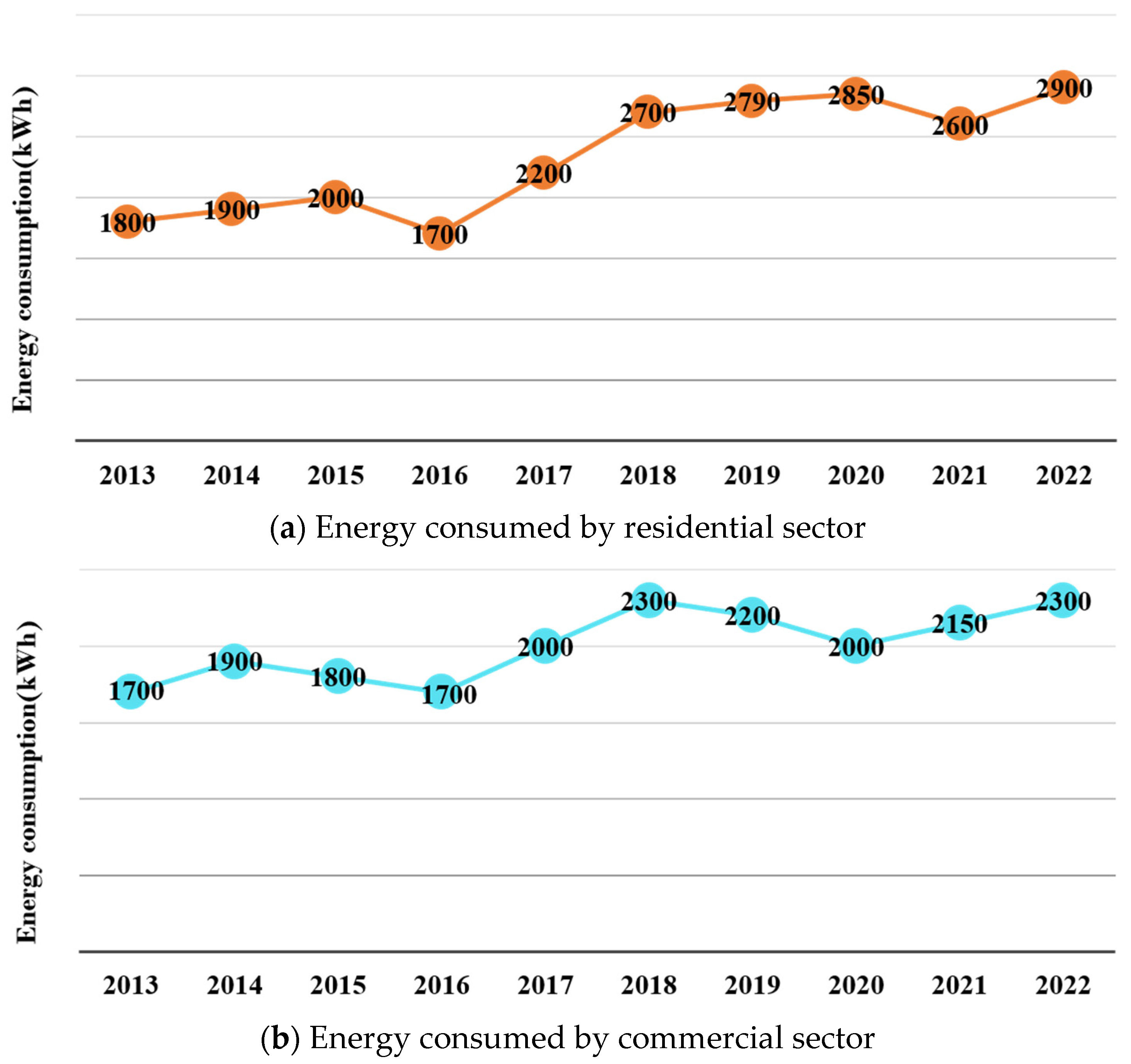
The COVID-19 pandemic, declared a global health crisis by WHO in March 2020, caused widespread deaths, impacted public health, economies, and energy safekeeping. From December 2022, WHO reported 99,057,629 confirmed COVID-19 cases and 1,080,010 deaths [1]. It led to a severe economic downturn, high unemployment, and a significant decline in GDP growth rates. The United States experienced energy security concerns, witnessing a 7% decrease in overall energy consumption, reaching 93 quads in 2020 compared to 2019, as per the EIA’s Energy Review [2]. The commercial and residential sectors saw a 7% decrease in energy consumption to under 17 quads in 2020. Home heating also decreased by 1% to under 21 quads due to warmer weather. This reduction was a result of lockdown measures, including closed offices, businesses, schools, industrial facilities, and limited recreational activities. In particular, home power sales in the U.S. increased by 8% in May compared to April 2019, while the commercial sector decreased by 11% [3]. The energy sector’s return to normalcy will be gradual, as shown in Figure 1, as studies indicate substantial changes in residential and commercial energy consumption due to COVID-19 lockdowns [4,5]. The pandemic remains an ongoing source of uncertainty, particularly in sectors closely tied to human life. With governments and societies worldwide relaxing policies and focusing on economic recovery post-omicron wave, there is also the looming risk of new variants. Accurate energy consumption forecasting is crucial for ensuring energy security, social operations, and a safe living environment in the face of challenges.

Figure 1.
Energy consumed by commercial and residential sector from January 2000 to February 2023.
Long-term, medium-term, and short-term forecasting are commonly used divisions when it comes to predicting energy consumption [6,7]. Let us delve into each division in more detail: Short-term forecasting focuses on predicting energy consumption within relatively brief intervals, usually ranging from one hour to one week. This forecasting horizon includes hourly, daily, and weekly predictions. The aim here is to provide accurate and timely insights into energy usage patterns in the immediate future. Moving on to medium-term forecasting, this approach is employed to forecast energy consumption over slightly longer intervals, typically spanning from 1 week to 1 year. Monthly and quarterly horizons are commonly utilized in this type of forecasting. The objective is to gain a broader understanding of energy consumption trends and patterns that extend beyond the immediate short term. Lastly, long-term forecasting is employed for predicting energy consumption over periods exceeding one year. This approach is used for annual horizons or even longer durations. By analyzing historical data and considering various influencing factors, long-term forecasting seeks to provide insights into future energy consumption [8]. The prediction of individual customers’ energy usage in networks with smart grids has received little attention from models and algorithms. Traditionally, energy use for the following day, hour, week, month, and year was the main focus. Due to the lack of historical data and the limits of algorithms, the prediction of current customers’ energy use is more manageable than the prediction of future demand. Even if each customer has an individual energy need, residential consumers still exhibit a consistent pattern of energy usage [9]. As a result, it is difficult for researchers and experts to predict the energy consumption of specific customers in networks of smart grids [10].
1.2. Related Work
A review of pertinent articles was carried out on energy consumption forecasting and efficiency enhancements. These studies look at household and commercial building energy efficiency models. Due to the complex structure and numerous hidden layers, deep learning techniques have been applied in the literature on energy consumption prediction. Deep learning techniques are expensive to apply with large datasets due to the training times of the algorithms. At the moment, grey system models, statistical forecasting simulations, machine learning approaches, and deep learning models can all be used to predict energy use. The most established forecasting techniques are time series models. Numerous researchers have made significant advancements in energy consumption forecasting in the previous few years by broadening the scope of conventional time-based approaches at the application and modeling stages [11]. For instance, various specialized time series forecasting models have been recommended for specific applications. In Turkey, the SARIMAX (seasonal autoregressive integrated moving average with exogenous factors) is often used to predict natural gas utilization in residential sector. When dealing with short-term gas consumption forecasts, the recursive autoregressive model with additional input is favored. Additionally, the WT-ARIMA model (wavelet transform autoregression integrated moving average) finds its utility in load forecasting [12,13]. These models are designed to account for trends, seasonality, and chronological patterns in the facts, making them suitable for various forecasting horizons. However, it is important to note that when dealing with large-scale data characterized by complex nonlinearities, certain limitations may arise. In such cases, time series models tend to demonstrate more robust performance in medium- and long-term forecasting scenarios as opposed to short-term predictions.
In recent years, grey system models have become increasingly popular for energy forecasting, especially when handling nonlinear time series data. Researchers have developed a number of models to forecast energy use in various regions and nations. An improved nonlinear grey Bernoulli model, for instance, was developed by Khan and Osinska [14] specifically for predicting energy consumption in India and Brazil. A seasonal adaptive grey model was developed by Ding et al. [15] to anticipate medium-term renewable energy consumption with an emphasis on the US commercial sector. The grey Lotka-Volterra model was additionally proposed by Zhang et al. [16] to investigate the core links among the energy utilization systems in the United States, China, and Deutschland. The ideal nonlinear metabolic grey system approaches were proposed by Chen et al. [17] and were created especially for predicting energy consumption in the Yangtze River Delta area. In order to predict the portion of renewable energy within main energy utilization, an insignificant nonlinear grey Bernoulli approach with systematic capabilities was projected [18]. Additionally, combining the “grey box” technique with additional nonlinear methods has the potential to solve problems related to nonlinear long-term forecasting. Despite these developments, it is important to note that the use of grey scheme models for intermediate and short-term prediction has been fairly restricted and frequently leads in less accurate [7].
When it comes to medium- and short-term prediction, data-driven ML approaches are favored over traditional time-based models and the grey system technique. The reason behind this preference is that machine learning models require learning from the data and hyperparameter tuning to develop an effective forecasting capability. Unlike their counterparts, these models have the ability to adapt and make accurate predictions. Today, many academics rely on machine learning models for energy forecasting. These models provide precise predictions by leveraging the power of advanced algorithms and techniques. By directly utilizing machine learning models, researchers are able to enhance the accuracy and reliability of their forecasts. An alternative study technique that has gained popularity involves employing different machine learning (ML) models for energy forecasting and evaluating the accuracy of their predictions [19,20]. To predict solar and wind power in the short to medium term, Gaussian process regression has been employed [21]. However, extensive research has revealed that hybrid approaches outperform individual models. For instance, hybrid models combining SVR [22,23], extreme gradient boosting (XGB) [24], and multiple machine learning models [25] have demonstrated superior performance. Machine learning models offer several advantages for short- and medium-term forecasting, particularly their ability to tackle complex nonlinear problems. However, when it comes to monthly and quarterly forecasts, these models face limitations and often exhibit a “time delay” issue, resulting in lower prediction accuracy. In the domain of energy consumption predictions, various neural network models are widely employed due to the popularity of deep learning techniques.
Deep learning (DL) approaches are driven by data and require substantial amounts of training data to optimize their hyperparameters, similar to traditional ML models. Consequently, DL models are commonly utilized for short-term and intermediate-term forecasting, primarily due to their exceptional precision, resilience, and remarkable capacity to handle entirely nonlinear problems. Currently, the long short-term memory (LSTM), the recurrent neural network (RNN), the convolutional neural network (CNN), and the gate recurrent unit (GRU) are widely recognized as the utmost widespread neural network approaches. These models have been extensively studied and utilized in various research endeavors. Ding et al. [26] developed a prediction model for renewable energy production by utilizing Loess (STL) and LSTM. In order to estimate the supply of renewable power in the Asian country South Korea, a hybrid model combining LSTM and variational autoencoder was proposed [27]. Yang et al. [28] employed a nonlinear mapping system to predict wind energy utilization. Amalou et al. [29] conducted an evaluation of LSTM, RNN, and GRU in various methods for energy utilization forecasting. Multiple studies have shown that integrating neural networks with multiple layers can effectively enhance the predictive capabilities of individual neural networks, such as the LSTM-RNN [30]. Other successful approaches include CNN-GRU [31], A-CNN-LSTM (where A represents the attention layer) [32], RNN-LSTM [33], CNN-BiGRU [34], LSTM-GAM [35], ConvLSTM-BDGRU-MLP, and CNN-LSTM [36]. Table 1 illustrates the diverse landscape of energy consumption forecasting techniques, outlining their key traits, advantages, and limitations across various modeling approaches.

Table 1.
Summary of energy consumption forecasting techniques and their characteristics.
1.3. Contribution
These research findings highlight the effectiveness of combining neural networks with different layers to improve prediction accuracy. According to the study, CNN and LSTM are highly regarded for their effectiveness in identifying data features [37]. Notably, the bidirectional LSTM (BiLSTM) has shown superior performance in predicting energy usage when compared to alternative models. The researchers suggest a hybrid model that fuses CNN and BiLSTM to forecast energy consumption in both the residential and commercial sectors.
Integration of Novelty
Our research pioneers a fresh approach to energy consumption forecasting, employing advanced deep learning algorithms. In contrast to conventional methods, our unique approach leverages diverse sensor data, enabling precise estimations of individualized energy consumption. A key breakthrough lies in our ability to predict energy needs tailored to specific customers within smart grid systems—an area largely overlooked in prior studies. Our exploration encompasses both residential and commercial sectors, aiming not only to optimize grid efficiency but also to empower proactive energy management strategies for a more sustainable future.
1.4. Paper Organization
Within this manuscript, we embark on an exploration aimed at enhancing building energy efficiency through the innovative integration of IoT-driven hybrid deep learning models for accurate energy consumption prediction. This endeavor unfolds across several sections, each contributing a pivotal facet to our comprehensive study. Commencing with the “Introduction”, we lay the groundwork by elucidating the motivation behind this research, delving into related works in the domain, and presenting the unique contributions that define our study. In “Materials and Methods”, Section 2, we delve into the technical aspects, delineating the methodologies employed, encompassing the extraction of spatial features using convolutional neural networks (CNN), temporal feature extraction with BiLSTM, and the design of our proposed CNN_BiLSTM model, complemented by insights into the grid search method utilized for hyperparameter fine-tuning. Section 3, “Experimental Setup and Analysis”, provides a detailed overview of the data acquisition process, comparative models used for evaluation, and an in-depth analysis of the forecasted outcomes. Following this, Section 4, “Discussion”, synthesizes our findings, elucidating the implications and significance of our results. Finally, “Conclusion and Future Work” in Section 5 encapsulates the study’s conclusions and outlines avenues for future research. This manuscript, thus, navigates a structured trajectory, culminating in comprehensive insights and potential directions to advance the realm of energy consumption prediction in building efficiency.
2. Materials and Methods
2.1. Extracting Spatial Features Using Convolutional Neural Networks
The energy consumption patterns in commercial and residential sectors exhibit nonlinear and nonstationary characteristics, which are influenced by the geographical locations of these areas. Capturing these spatial features poses a challenge, though the CNN provides an effective solution by effectively learning the configuration of the time series-based data. CNNs are neural networks that utilize convolutions to simplify the complexity of the network. The key operations of CNNs are local feature extraction and weight sharing. Given that the spatial relationship within the time-based/series data is localized, every neuron in the network barely needs to focus on capturing resident features. By combining these local neurons, global information can be obtained, thereby reducing the number of associations required. Weight sharing further enhances the adaptability and simplicity of the network by reducing the hyperparameters. The main components of a CNN responsible for feature extraction are the convolutional layer and the pooling layer. These modules work together to extract relevant features from the input data. The main focus of this paper is to analyze the spatial characteristics of time series data through the use of convolutional layers. Unlike traditional weight connection layers, these layers apply the convolution technique to extract relevant features. Specifically, this paper utilizes the 1D-convolution layer to perform this task. During a convolution operation, a convolution kernel glides over the input (i/o), computing the innermost product with the i/o to generate a novel feature matrix. This process aids in capturing the spatial properties of the time-oriented data. Given a 1D i/o of time stamp , the output (o/p) generated by the convolution layer using a single convolution kernel is represented as . Equation (1) shows the mathematical formula of a convolutional layer using single convolution kernel.
In this approach, the subsequence “” represents the i/o roofed by the pth slide of “”, while “” denotes the kernel scope. Since the input is one-dimensional, the convolution kernel has a single network. Consequently, the output size represented in Equation (1) is determined solely by the kernel scope and i/o range.
By reducing the number of features, the pooling layer is an essential component for feature matrix compression and the avoidance of overfitting. The two frequently used techniques of maximum pooling and average pooling are in use inside this layer. When using the feature matrix, maximum pooling, produced by the convolution layer, is divided into subdivisions, and the highest value is chosen from each of these subregions. A new feature matrix with fewer dimensions than the original is produced as a result of this operation. Finding the most responsive feature components is where max pooling really shines. In contrast, average pooling produces a changed feature matrix by calculating the mean value inside each subregion. This method conserves the inclusive features of the data while reducing the variances between the features. In summary, the pooling layer plays a crucial role in compressing the feature matrix and avoiding overfitting. Max pooling focuses on extracting the most responsive features, while average (avg) pooling maintains the inclusive features of the data point. Therefore, this paper utilizes the 1D max pooling layer. It assumes that the i/o range of the max pooling tensor is , where refers to the number of channels or feature maps in the input, represents the number of classes or categories, and signifies the length or size of the input. The output can be described using the following formula shown in Equation (2):
In this equation, the output at position is obtained by taking the maximum value over a sliding window of size k along the input tensor. The gliding window moves with a stride of . The index iterates over the elements of the gliding window. The o/p range is , where is calculated as shown in Equation (3):
Here, represents the length or size of the output tensor along the input dimension. It is computed by subtracting the size of the sliding window from the input size .
2.2. BiLSTM-Based Temporal Feature Extraction for Time Series
LSTMs have proven to be effective for time series forecasting due to their ability to accurately capture long-term dependencies. Over the years, various variants and versions of LSTM have emerged, showcasing outstanding performance. One widely applied LSTM variant is the BiLSTM, developed by Schmidhuber [38], which consistently outperforms traditional LSTM approaches in time series prediction. Therefore, this work leverages the BiLSTM model to enhance forecasting performance. Firstly, let us delve into the workings of the basic LSTM. Then, we will explore the operations of BiLSTM. The output of an LSTM depends on three factors at distinct times, as depicted in Figure 2.
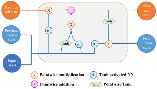
Figure 2.
Working model of long short-term memory (LSTM).
Firstly, the neural network stores long-term information in the present—known as the cell state. Secondly, it retains the output from the last state—referred to as the previous hidden state. Lastly, it incorporates the input data for the current time step. LSTMs employ a series of “gates” to regulate data flow within the network, controlling how information enters, remains, and exits. The conventional LSTM architecture encompasses three gates: an output gate, an input gate, and a forget gate. These gates function as individual neural networks or filters, each serving a distinct purpose. The input gate allows pertinent data to be extracted from the current cell state. Utilizing the sigmoid activation function, this gate determines which data are necessary for the current input and which can be disregarded. Subsequently, the data are stored in the current cell state. Following this step, the tanh activation mechanism computes vector representations of the input gate values, which are then added to the cell state [39]. Equations (4) and (5) depict the computational formulae for the input gate and the current cell state.
where is the input gate; is the previous hidden state; is the current cell state. The forget gate is the initial stage of the procedure. Considering the initial concealed state and fresh input data, the forget gate determines the utility of specific cell state bits. The NN receives both the original hidden state and the new input data. Each element within the vector generated by the network falls within the range of [0, 1]. It is helpful to conceptualize each component of the vector as a filter, allowing more information to pass through as its value approaches 1. These output values are then scaled by the initial cell point before advancing. Through point-wise multiplication, components of the cell state deemed irrelevant by the forget gate network, multiplied by values near zero, subsequently exert lesser influence in subsequent steps. Here, h(t − 1) signifies the resulting concealed state at timestamp (t − 1). The input x(t) and output h(t − 1) are initially derived by the forget gate, which subsequently employs point-wise multiplication of its weight matrix alongside the addition of sigmoid activation to determine the probability scores. It can distinguish between relevant and beneficial information using likelihood scores. The forget gate is represented as below in Equation (6):
The output gate determines the current cell state, and the weights in the output gate matrix are maintained and updated through backpropagation. A point-wise multiplication operation is conducted on the weight matrix using the input/output token x(t) and the previous output h(t − 1) from the hidden state. As mentioned earlier, this occurs atop a sigmoid activation since it necessitates probability calculations to determine the output order. Once sigmoid results are obtained, they are multiplied by the new cell state, providing the necessary information to predict the final output. To ensure that the numerical range remains within [−1, 1], our output sequence is completed after the final multiplication with tanh. Equation (7) shows how output sequence is calculated mathematically. Equation (8) represents the mathematical formula of hidden state.
where denotes the output gate and is the hidden state.
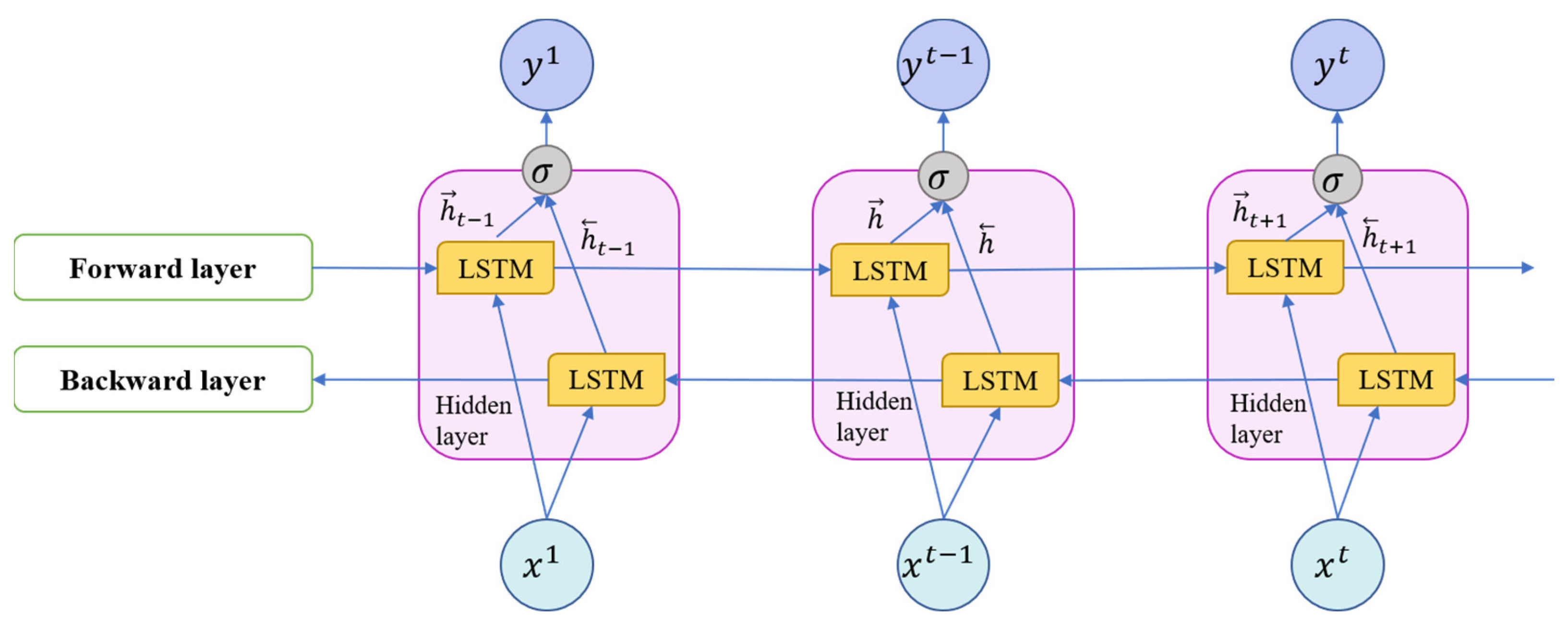
Algorithm 1 illustrates the complete implementation process of the LSTM, utilizing all three gates of the LSTM to calculate annual electricity consumption. The architecture of the BiLSTM network is depicted in Figure 3. It is important to note that the standard one-directional LSTM differs from the bidirectional long short-term memory (BiLSTM), which comprises two distinct LSTM structures. These structures employ both the forward and reverse order of the input data to learn features. This unique characteristic enables the model to undergo training from both input to output and output to input. Consequently, this feature significantly enhances the model’s dependency and augments its forecasting accuracy. In the case of BiLSTM, the hidden layer () comprises both the forward hidden state () and the backward hidden state (), which can be represented as follows:
| Algorithm 1. Long short-term memory (LSTM). |
| Input: Normalized input data Output: Predicted annual electricity consumption of the residential building
|
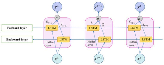
Figure 3.
The architecture of the BiLSTM network.
2.3. Proposed CNN_BiLSTM
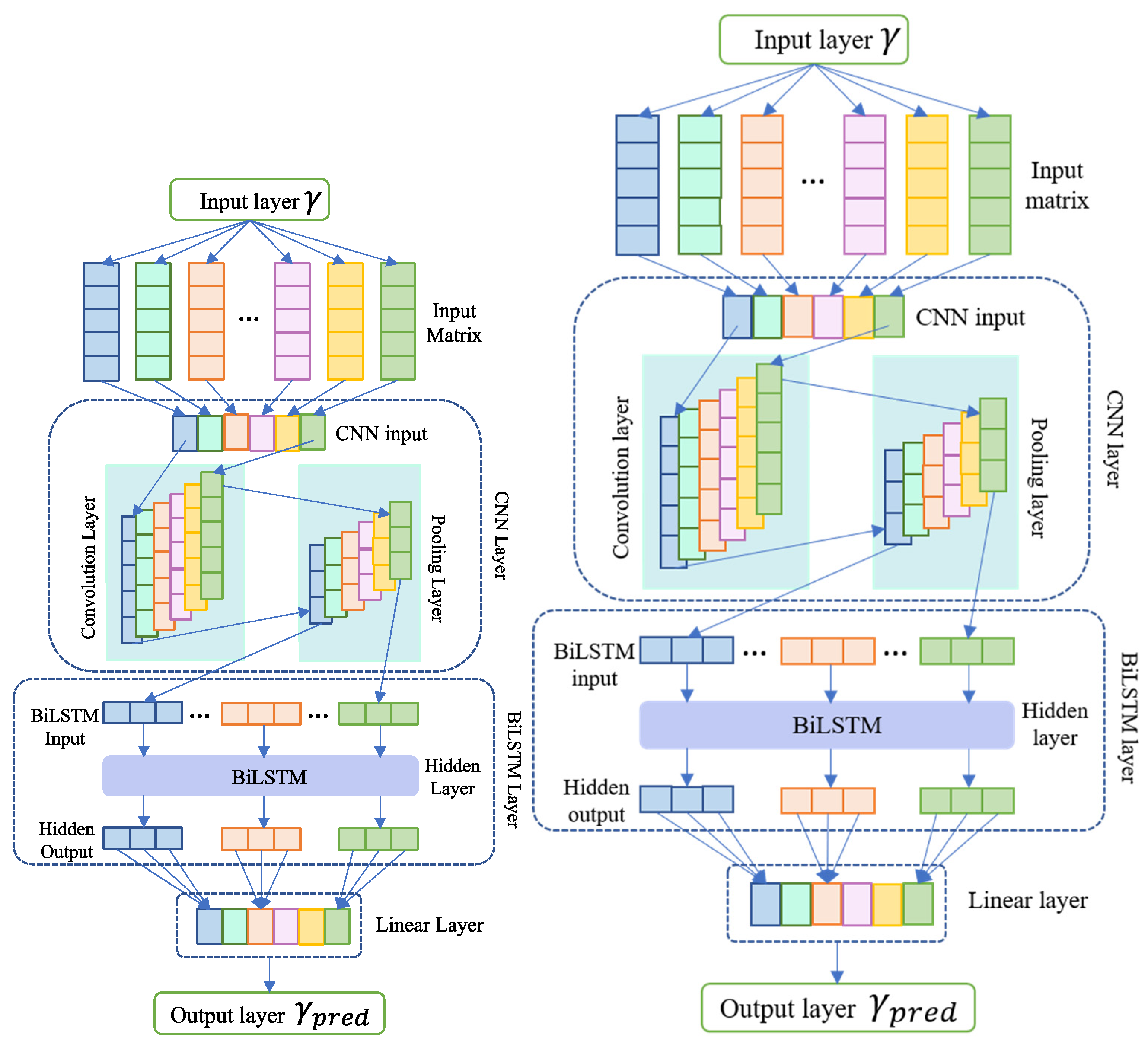
A proposed model for predicting energy utilization in commercial and residential sectors is the CNN_BiLSTM hybrid technique. This model associates the BiLSTM, CNN, and a joining layer. Initially, the convolutional layer takes the input within the CNN_BiLSTM model, performing convolution computations and employing max pooling to generate a new feature matrix. This matrix derived from CNN operations serves as input for the subsequent BiLSTM layer, generating hidden outputs that encapsulate temporal dependencies within the energy consumption data. These hidden outputs are then processed through an interconnected layer comprising a linear layer, responsible for deriving concealed output. Finally, the connection layer produces the ultimate projected results, elucidating the relationship between input and output through the hybrid CNN_BiLSTM model. The fusion of CNNs and BiLSTMs in the CNN_BiLSTM model holds significant theoretical grounding in enhancing predictive accuracy, particularly in forecasting weekly energy consumption patterns. CNNs excel in extracting spatial or temporal patterns from input data through convolutional and pooling layers. In energy utilization prediction, CNNs efficiently capture local dependencies and patterns in the temporal data, discerning meaningful features representing various patterns like hourly or daily fluctuations in energy usage. The pivotal integration of the BiLSTM layer further strengthens the model’s predictive capabilities. BiLSTMs, a variant of recurrent neural networks (RNNs), capture long-range dependencies and sequential patterns, considering both past and future context simultaneously. This proves advantageous in energy consumption forecasting, where dependencies exist not only in recent historical data but also in longer-term trends such as weekly or monthly patterns. The synergy between CNNs and BiLSTMs addresses individual architecture limitations. While CNNs focus on local patterns, BiLSTMs specialize in capturing long-term dependencies, enabling a comprehensive analysis of energy utilization patterns at various temporal scales. The convolutional layers extract hierarchical features, contextualized by the bidirectional temporal modeling of the BiLSTM layer. By effectively leveraging both spatial and temporal information, the CNN_BiLSTM model accurately captures complex energy consumption patterns on a weekly basis. This integration enables adaptive learning and utilization of multiscale features, significantly enhancing precision in forecasting weekly energy utilization in both commercial and residential sectors. The detailed calculation process of the proposed work is elaborated in Algorithm 2:
| Algorithm 2. The CNN_BiLSTM algorithm. |
| Input: Let be the input time series of length n. Let be the corresponding output time series of length m. Output: Predicted energy consumption of the residential and commercial building.
|
The workflow of the CNN_BiLSTM can be observed in Figure 4.
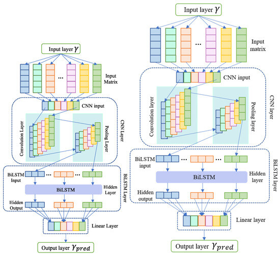
Figure 4.
The proposed CNN_BiLSTM network.
2.4. Grid Search Method for Fine-Tunning CNN_BiLSTM Hyper-Parameters
Neural networks are known for their complexity in configuration, often necessitating the adjustment of numerous hyperparameters. It is widely recognized that the effectiveness of a deep learning technique is comprehensively influenced by the choice of hyperparameters. In recent years, swarm intelligence optimization methods have gained considerable popularity for the purpose of fine-tuning these model hyperparameters. Optimizing precision in various applications is influenced by several critical factors. These factors encompass the computational burden, fine-tuning of algorithmic parameters, convergence rate, and control mechanisms, among others. For instance, consider the widely recognized particle swarm optimization (PSO) technique, which often encounters limitations in local exploration, leading to suboptimal convergence rates and ultimately reduced precision or outright failure [40]. To address these challenges, the grid search method emerges as a popular and direct approach for efficiently fine-tuning model hyperparameters. It has proven successful in optimizing the hyperparameters of deep learning models [41]. Consequently, the grid search method serves as a valuable tool for tailoring the ideal hyperparameters of models. The proposed work for hyperparameter optimization using grid search consists of two primary components: the grid search scheme and data division. To mitigate overfitting issues in time series forecasting, we employ nested cross-validation [42] for data partitioning.
This method is widely recognized for hyperparameter optimization and model selection. The dataset is divided into three distinct portions. Training data (): This segment, which comprises 80% of the dataset, is dedicated to model fitting. It involves the utilization of input data () and corresponding output data () to construct the predictive model. Validation data (): Accounting for 10% of the dataset, this set is reserved for model validation. It facilitates the evaluation of the model’s generalization to unseen data. Input data () and output data () in this section play a pivotal role in fine-tuning the model’s hyperparameters. Testing data (): The remaining 10% of the data are allocated for testing purposes. This portion ( and ) is crucial for assessing the out-of-sample forecasting performance of the model, providing a realistic measure of its real-world effectiveness. By adopting this structured approach to data division and integrating it with the grid search strategy, the objective is to effectively optimize hyperparameters and enhance the accuracy of the time series forecasting model. To determine the optimal hyperparameters for the proposed CNN_BiLSTM model, the grid search technique was employed, leveraging both the training and validation datasets. Within the scope of hyperparameter tuning, three critical parameters require adjustment: the learning rate (), a pivotal factor in deep learning model training; the hidden size () for the BiLSTM component; and the kernel size () for the CNN component. The fundamental principle underlying the grid search strategy is to systematically explore various combinations of these hyperparameters within a predefined grid. The primary objective is to minimalize the MSE (mean squared error) observed on the justification data, namely, and . Calculative expression of MSE is represented by Equation (10):
Upon selecting the optimal hyperparameters, denoted as , , and , the CNN_BiLSTM model undergoes a retraining process using the in-sample data, which mutually encompass the validation dataset () and the training dataset (). This retraining step is essential to ensure that the model is fine-tuned according to the selected hyperparameters. Subsequently, the model, now fitted with the optimal hyperparameters, is prepared for assessing its predictive performance using the assessment data (). In conclusion, the following algorithm summarizes the whole computational programming approach for hyperparameter tuning, which relies on the grid search approach.
3. Experimental Setup and Analysis
3.1. Data Acquisition and Preparation
The dataset utilized in this research, sourced from the EIA Monthly Energy Review, represents a comprehensive collection spanning an extensive timeframe from January 1973 to May 2020 [43]. The EIA Monthly Energy Review is a crucial publication by the U.S. Energy Information Administration, serving as a comprehensive repository for energy statistics and trends within the United States. This resource is instrumental in understanding and analyzing the nation’s energy landscape, aggregating a wealth of data related to energy production, consumption, prices, and key metrics across diverse sectors like residential, commercial, industrial, and transportation. Encompassing a substantial timeframe from January 1973 to May 2020, this publication provides detailed insights spanning almost five decades of energy consumption patterns and fluctuations within the U.S. energy sector. It includes a broad spectrum of statistics covering areas such as petroleum, natural gas, coal, electricity, renewable energy sources, and energy prices. Professionals ranging from researchers and policymakers to analysts and industry experts often rely on the EIA Monthly Energy Review for assessing energy consumption patterns, examining historical trends, and making well-informed decisions concerning energy policies and investments. This dataset boasts an impressive volume, encompassing over individual data points. It intricately captures nuanced trends in total energy consumption and provides detailed breakdowns across multiple sectors, including residential, commercial, primary, and end-use categories. To ensure coherence and meaningful analysis, the raw dataset underwent an essential preprocessing phase. Leveraging MinMax scaling, we normalized the diverse range of values, aligning them within a standardized scale confined to the [0, 1] range. This normalization strategy was pivotal, aiming to neutralize potential biases stemming from varying scales across distinct energy consumption metrics. It preserved the dataset’s inherent patterns and dynamics while facilitating fair and comprehensive model training. Furthermore, the dataset was meticulously partitioned into two distinct subsets to facilitate robust model evaluation. The first subset, encompassing data from June 2018 to May 2020, functioned as the testing dataset, allowing rigorous assessments of model performance in an out-of-sample scenario. Meanwhile, the second subset, spanning from January 1973 to May 2018, served as the in-sample dataset, enabling effective model training and hyperparameter optimization. The EIA Monthly Energy Review stands as a comprehensive repository, capturing intricate energy consumption trends over nearly five decades. Its expansive scope and granularity empower detailed analyses across various sectors, providing invaluable insights into the evolution of energy usage patterns over time. This dataset’s extensive coverage enhances the credibility and reliability of our research findings, establishing a robust foundation for assessing and validating the developed models. This meticulous approach not only enhances the manuscript’s credibility but also contributes to the robustness and generalizability of the developed models by establishing a solid foundation for their assessment and validation.
3.2. Comparative Models and Performance Metrics
To facilitate a comprehensive model comparison, a range of deep learning architectures, including convolutional neural networks (CNNs) [44], long short-term memory networks (LSTM) [45], and a combined CNN-LSTM approach [46], were developed in this study. Additionally, well-established machine learning models, such as gradient boosting with categorical feature provision (CatBoost), XGBoost [47], and light gradient boosting machine (LGBM) [48], were incorporated. To assess the predictive accuracy of these models, a set of evaluation metrics was employed. A detailed overview of these performance metrics is presented in Table 2, providing a comprehensive reference for the assessment criteria.
Table 2.
Assessment metrics for evaluating the predictive performance of the CNN_BiLSTM model.
3.3. Analysis of Forecasted Outcomes
To conduct a comprehensive comparison between the CNN_BiLSTM model and other models, four distinct comparisons were performed. These comparisons encompassed the assessment of total energy consumption within both the residential and commercial sectors, as well as the evaluation of results achieved using performance metrics specific to each of these sectors. The comparison is visually represented using graphics—a graph displaying the energy consumption range in kilowatt-hours (KWH) across varying numbers of test cases, indicated on the x-axis from 1 to 24. The y-axis depicts the range of energy consumption values in KWH. As the number of test cases increases, the bar heights demonstrate the fluctuation in energy consumption, showcasing the variability in KWH across the different scenarios tested.
3.3.1. Residential Sector Energy Consumption Analysis
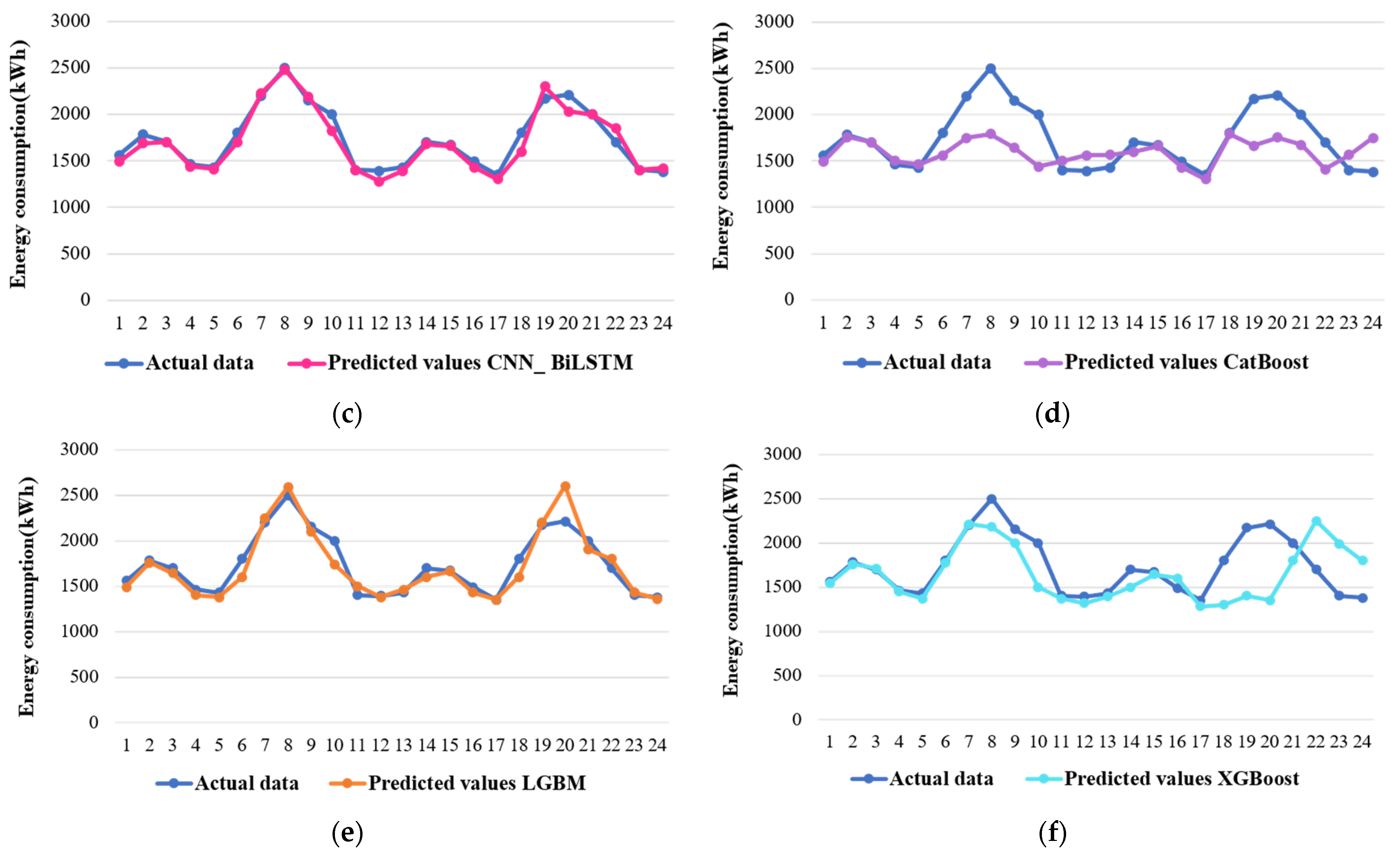
In the context of predicting entire energy consumption by the residential area, Figure 5 showcases the proposed algorithm’s predicted values. A notable observation is that the forecasted values generated by the CNN_BiLSTM model closely align with the raw data. Furthermore, the forecasted curve of the BiLSTM model bears a resemblance to that of the CNN_BiLSTM, which is expected since the BiLSTM constitutes single layer within the CNN_BiLSTM architecture, though it is worth noting that the BiLSTM model encountered challenges in forecasting the last two data points. A significant performance gap becomes evident when comparing the CNN_BiLSTM with the standalone CNN model. The hybrid CNN_BiLSTM model clearly outperforms the CNN, underscoring the effectiveness of the hybrid approach in enhancing predictive performance compared to a single-model strategy. On the other hand, the predicted values generated by other deep learning models exhibit a distinct pattern. These models appear to produce predictions akin to constants, reflecting an evident overfitting issue. In contrast, among the machine learning models, the light gradient boosting machine (LGBM) performs admirably in this context. However, the CatBoost and XGBoost models only manage to capture the general trend of the raw data, falling short in accurately forecasting the finer details. In summary, the CNN_BiLSTM model emerges as a robust performer in predicting residential sector energy consumption, demonstrating its superiority over other models, particularly in comparison to the standalone CNN model, which struggles to match its predictive prowess.
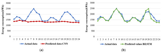
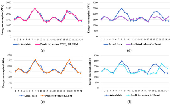
Figure 5.
Comparison of predicted and actual residential sector energy consumption of all the models: (a) CNN, (b) BiLSTM, (c) CNN_BiLSTM, (d) CatBoost, (e) LGBM, and (f) XGBoost.
The CNN_BiLSTM demonstrates superior performance compared to the other models, with consistently better metrics across the board. While the predicted values of light gradient boosting machine (LGBM) exhibit similarities to the CNN_BiLSTM, their corresponding metrics fall short in comparison. Furthermore, it is evident that the forecast accuracy achieved by the CNN_BiLSTM significantly surpasses that of both the individual CNN and BiLSTM models.
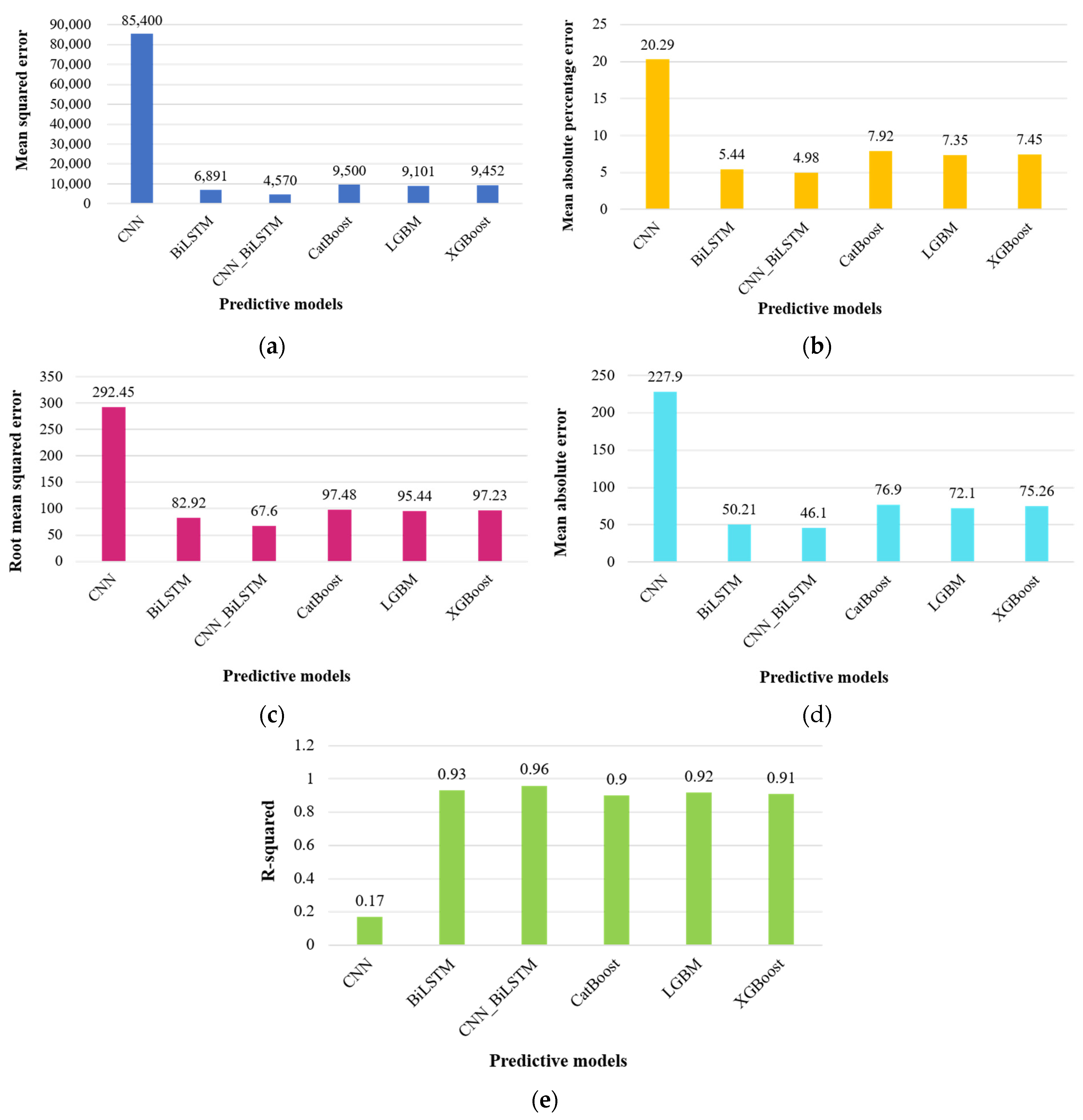
For the end-use energy consumption within the residential part, Figure 5 illustrates the predicted values, while Table 3 and Figure 6 provides the equivalent assessment metrics. Notably, as the number of forecasting steps increases, the prediction accuracy of most models tends to deteriorate. However, the CNN_BiLSTM model exhibits remarkable stability throughout this process. Comparatively, the CNN_BiLSTM consistently outstrips both the standalone CNN and BiLSTM models, despite the BiLSTM’s predicted values closely resembling those of the CNN_BiLSTM. This performance discrepancy becomes particularly evident in the later forecasting points, where the BiLSTM model’s stability falters in comparison to the CNN_BiLSTM.
Table 3.
Evaluation metrics for forecasting residential sector energy consumption.
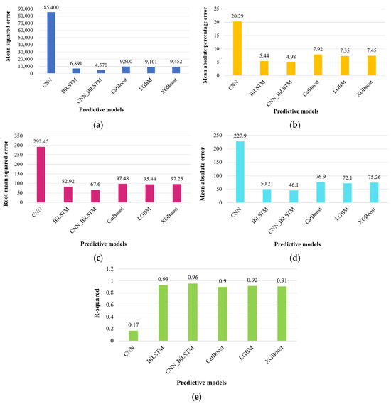
Figure 6.
Graphical representation of evaluation metrics for forecasting residential sector energy consumption: (a) mean squared error, (b) mean absolute percentage error, (c) root mean squared error, (d) mean absolute error, and (e) R-squared.
3.3.2. Commercial Sector Energy Consumption Analysis
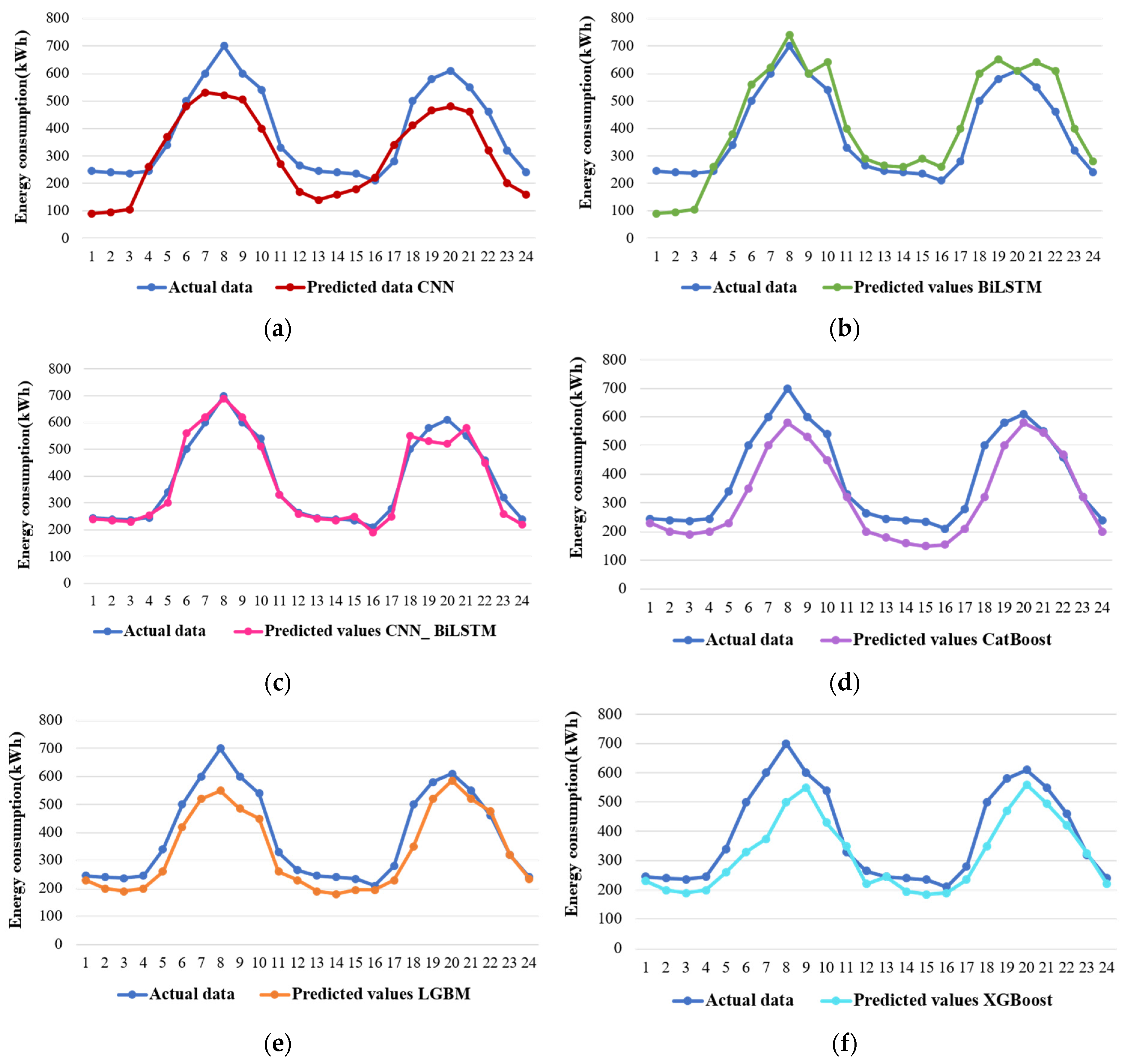
Figure 7 presents a visual comparison between actual energy consumption values and the predicted values for the commercial sector, while Table 3 provides an overview of the evaluation metrics. Overall, the CNN_BiLSTM model outperforms other predictive models, demonstrating its proficiency in predicting energy usage, with projected values closely aligning with real data samples. Notably, the CNN_BiLSTM model significantly enhances prediction accuracy when compared to individual deep learning approaches, containing CNN, BiLSTM, and LSTM.
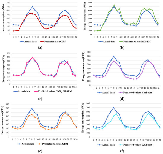
Figure 7.
Comparison of predicted and actual commercial sector energy consumption of all the models: (a) CNN, (b) BiLSTM, (c) CNN_BiLSTM, (d) CatBoost, (e) LGBM, and (f) XGBoost.
The efficiency of the CNN_BiLSTM model in forecasting is evident in Figure 7. When we examine the anticipated values generated by deep learning models (depicted in (a)–(f)), it is clear that the CNN approach presents poorly in forecasting. The predicted values deviate significantly from the actual values, mainly due to overfitting issues. Additionally, the CNN model fails to capture the ongoing periodic patterns and exhibits an inaccurate linear growth trend in its predictions, which is a consequence of its overfitting nature. In contrast, when we compare it to the sole BiLSTM approach, the combination of BiLSTM with CNN demonstrates better-quality forecasting capabilities. It handles fluctuations more effectively and closely follows the original trend, showcasing its ability to provide more accurate and stable predictions. Concerning machine learning models, a common issue often encountered is the delay in predicted values, particularly as we move further ahead in the forecast timeline. These models tend to struggle when it comes to accurately predicting values in close proximity to topmost points. In comparison, the CNN_BiLSTM approach displays a notable improvement in professionally capturing these peak points. It exhibits a pattern of predicted values that closely aligns with the original data, displaying less of a “lag” feature when forecasting energy consumption. This suggests that the CNN_BiLSTM technique excels in providing timely and accurate predictions, especially in critical periods of energy consumption.
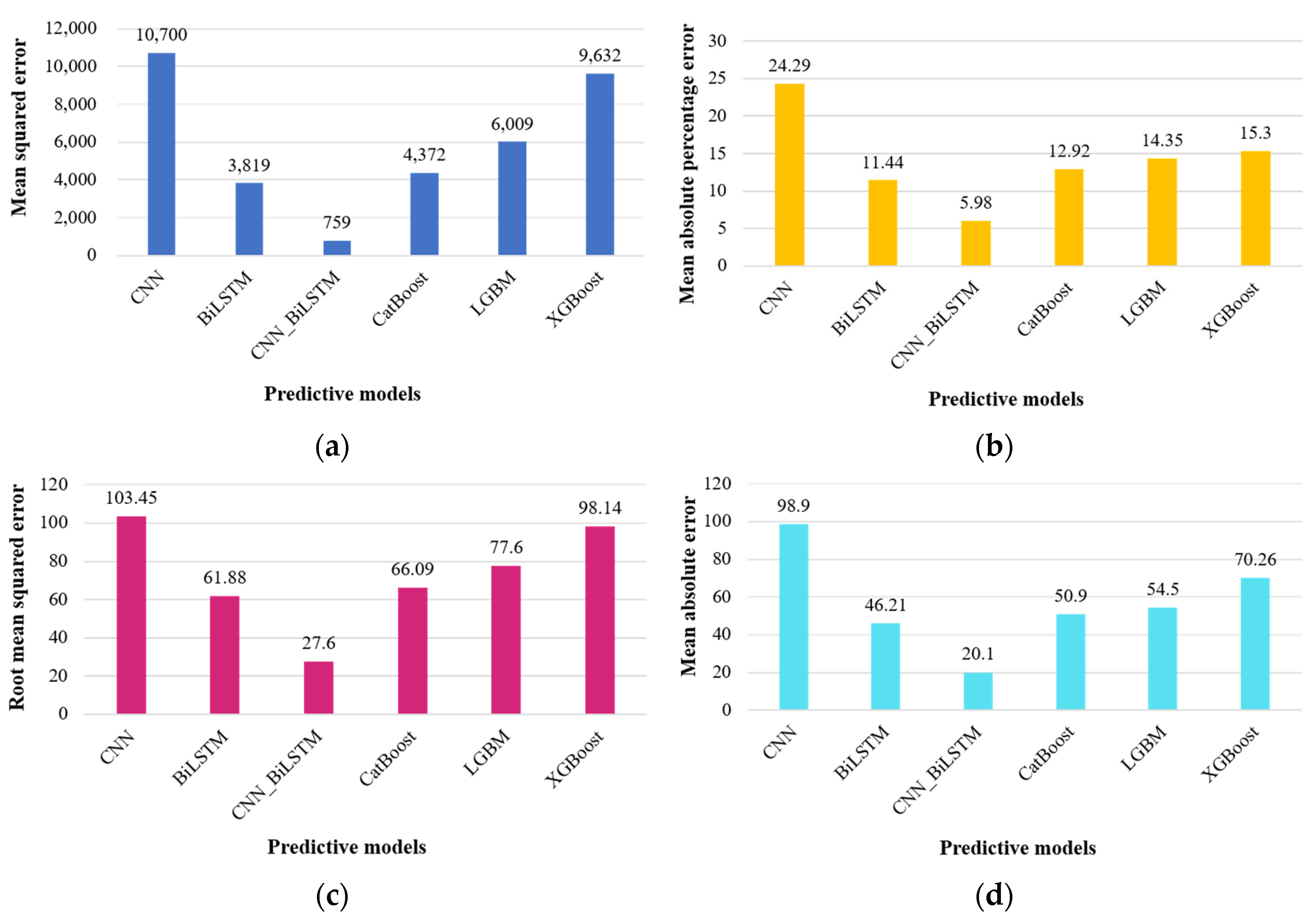
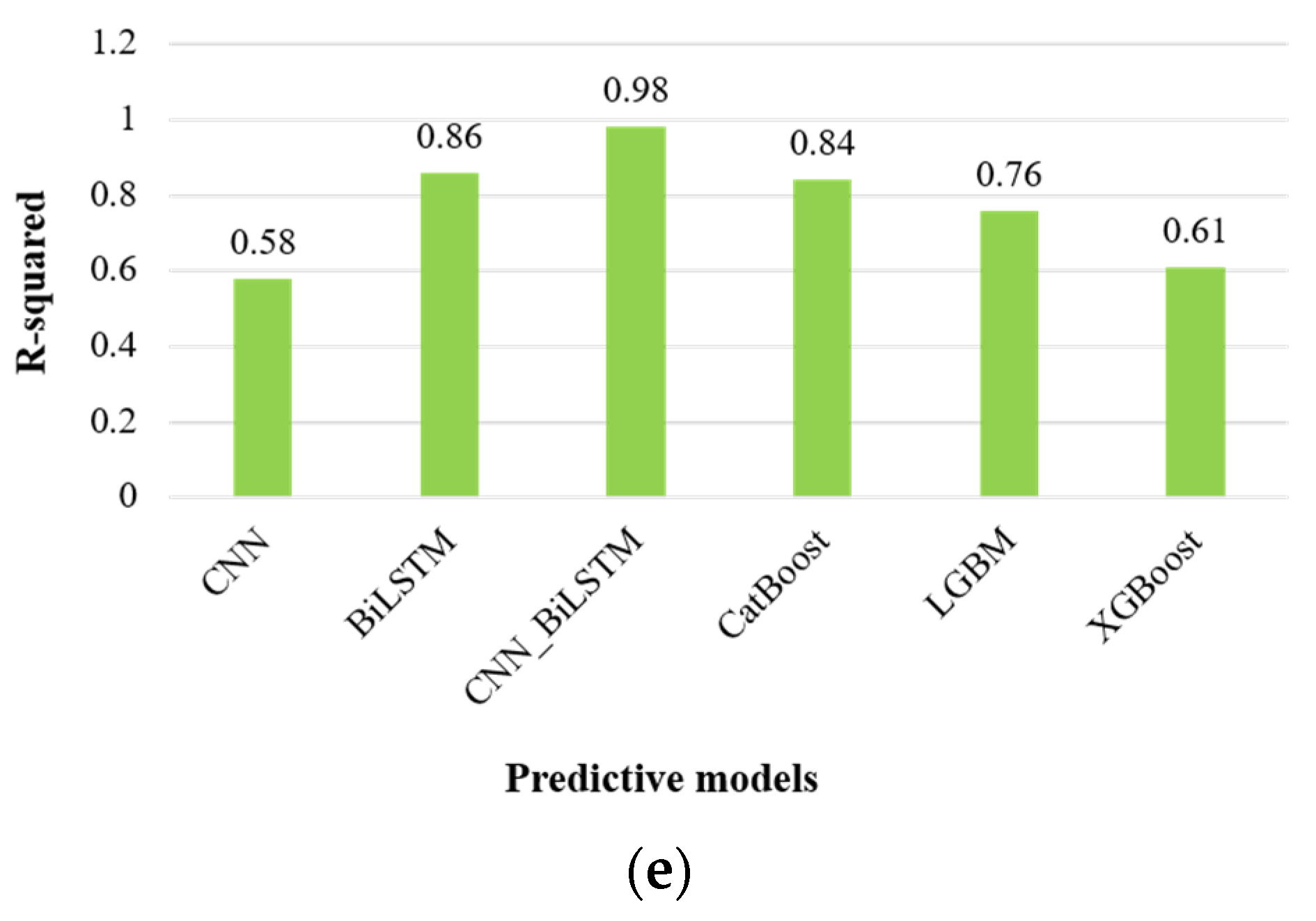
In terms of the evaluation metrics provided in Table 4, and graphical representation in Figure 8, the CNN_BiLSTM model consistently yields superior results, indicated by its larger R-squared (R2) values compared to other machine learning and deep learning techniques. Notably, the R2 values for the supplementary deep learning techniques are comparatively modest, particularly the CNN model, which has an R2 value of 0.58. In contrast, our proposed CNN_BiLSTM model exhibits a significantly higher R2 value of 0.98, underscoring its remarkable ability to generate accurate forecasts and achieve favorable outcomes.
Table 4.
Evaluation metrics for forecasting commercial sector energy consumption.
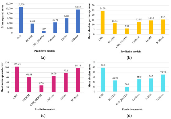

Figure 8.
Graphical representation of evaluation metrics for forecasting commercial sector energy consumption: (a) mean squared error, (b) mean absolute percentage error, (c) root mean squared error, (d) mean absolute error, and (e) R-squared.
When comparing with benchmark deep learning models, the CNN_BiLSTM model stands out, displaying a significantly lower MAPE, which is reduced by approximately five times compared to these models. The reduction in MAPE ranges from 5.98% to 24.29%. In contrast, the machine learning models’ predictive capabilities fall short in comparison to the CNN_BiLSTM model. In summary, the CNN_BiLSTM consistently delivers superior forecasting performance.
4. Discussion
The CNN_BiLSTM model consistently outperforms other DL and ML models, closely aligning its predicted values with the actual data trends across all cases. In the subsequent sections, we provide a more detailed analysis of the model’s predictive capabilities and its performance in various applications. In recent years, the realm of predictive modeling and forecasting has witnessed significant advancements. Among the methodologies employed, tree models like random forest (RF) and CatBoost, as well as kernel models such as support vector regression (SVR) and least squares support vector regression (LSSVR), have consistently shown promise in tackling forecasting challenges in the past. These machine learning models have demonstrated effectiveness, especially when dealing with outliers and extreme data points that often deviate markedly from the original dataset. Nonetheless, it is intriguing to note that the CNN_BiLSTM deep learning model has emerged as a standout performer in addressing these intricate challenges. This deep learning architecture exhibits robust and stable performance, underscoring its prowess in handling time series data. This article presents a comparative analysis between the BiLSTM technique and the conventional LSTM technique, particularly in the context of time series forecasting, with a specific focus on energy consumption prediction. Our findings consistently highlight the superior predictive capabilities of the BiLSTM model, aligning with prior research in the domain of deep learning models for time series analysis.
To delve into the nuances, the BiLSTM model employs a unique training strategy involving dual components: forward and reverse LSTM layers. This approach enhances the model’s ability for comprehensive feature extraction, providing a holistic perspective of the input sequence. While the forward LSTM captures past data information, the reverse LSTM extracts insights into future data trends. This dual perspective empowers the BiLSTM model to make more accurate and robust predictions in energy consumption forecasting. Furthermore, the integration of convolutional neural networks (CNNs) with the bidirectional long short-term memory (BiLSTM) architecture has yielded remarkable enhancements when compared to employing these models in isolation. The CNN_BiLSTM model has demonstrated impressive performance metrics, including a mean square error (MSE) of 4570.14, mean absolute percentage error (MAPE) of 4.98%, root mean square error (RMSE) of 67.60, mean absolute error (MAE) of 46.10, and an R-squared (R2) coefficient of 0.96. In stark contrast, the light gradient boosting machine (LGBM), renowned as one of the most proficient machine learning models for residential sector applications, yielded different performance metrics. Specifically, it recorded a mean square error (MSE) of 9100.86, a mean absolute percentage error (MAPE) of 7.35%, a root mean square error (RMSE) of 95.44, a mean absolute error (MAE) of 72.1, and an R-squared (R2) coefficient of 0.92.
These outcomes distinctly underscore the superiority of the CNN_BiLSTM model in achieving accurate energy consumption predictions when compared to the LGBM model. This amalgamation of CNN and BiLSTM not only showcases remarkable performance across various evaluation metrics but also holds the promise of significantly enhancing forecasting accuracy in a wide array of time series prediction scenarios.
5. Conclusions
Predicting energy consumption in both residential and commercial sectors is a vital task, but it becomes especially challenging due to the intricate temporal and spatial patterns inherent in energy consumption time series data. Conventional deep learning and machine learning approach often struggle to provide reliable forecasts in such cases. To address this, we propose a hybrid model called CNN_BiLSTM, combining bidirectional long short-term memory (BiLSTM) and convolutional neural networks (CNNs), in this research to anticipate energy usage in these sectors. The CNN_BiLSTM model leverages the CNN layer to capture spatial characteristics within the time series data and the BiLSTM layer to capture both long-term and short-term temporal patterns. We also employ recursive prediction with the CNN_BiLSTM model to enhance its forecasting capabilities. Hyperparameter tuning, facilitated by grid search, helps identify the optimal configuration for the CNN_BiLSTM model. We utilized raw energy consumption data spanning from January 1975 to July 2022 for the US residential and commercial sectors in our study. The model’s performance is notably impressive, with key metrics indicating its accuracy. These include a mean square error (MSE) of 4570.14, a mean absolute percentage error (MAPE) of 4.98%, a root mean square error (RMSE) of 67.60, a mean absolute error (MAE) of 46.10, and an R-squared (R2) coefficient of 0.96. These metrics underscore the CNN_BiLSTM superior forecasting capabilities compared to various other deep learning and machine learning models, highlighting its ability to surpass the performance of individual CNN and BiLSTM models. It is worth noting that the CNN-BiLSTM’s effectiveness is most pronounced when dealing with substantial datasets. However, due to its multilayer architecture and substantial parameter training requirements, it may not be the best choice for modeling smaller datasets.
Future Work
In steering future research, key pathways emerge. These include refining the CNN_BiLSTM architecture for scalability while preserving accuracy. Exploring external factor integration enhances adaptability. Adapting the model for real-time predictions enables proactive decision making. Lastly, assessing its transferability across diverse contexts ensures wider applicability. These avenues promise heightened precision and adaptability in energy consumption forecasting.
Author Contributions
Y.N.: Conceptualization, methodology, visualization; S.P.K.R.: Data curation, writing—reviewing and editing; G.W.: Software, writing—original draft preparation; Y.C.: Investigation, supervision; Z.C.: Writing—reviewing and editing; D.-E.L. and Y.M.: Validation, resources. All authors have read and agreed to the published version of the manuscript.
Funding
This work was supported by the National Research Foundation of Korea (NRF) grant funded by the Korea government (MSIT) (No.2022R1F1A1068374). This research was supported by Brain Pool program funded by the Ministry of Science and ICT through the National Research Foundation of Korea (NRF-2022H1D3A2A02082296). This work was supported by the National Research Foundation of Korea (NRF) grant funded by the Korea government (MSIT) (No. NRF-2018R1A5A1025137).
Institutional Review Board Statement
Not applicable.
Informed Consent Statement
Not applicable.
Data Availability Statement
The data and the code of this study are available from the first author upon request.
Conflicts of Interest
The authors declare no conflicts of interest.
References
- World Health Organization. WHO COVID-19 Dashboard; World Health Organization: Geneva, Switzerland, 2020; Available online: https://covid19.who.int/ (accessed on 26 June 2023).
- U.S. Energy Consumption Fell by a Record 7. Available online: https://www.eia.gov/todayinenergy/detail.php?id=47397 (accessed on 26 June 2023).
- Stay-at-Home Orders Led to Less Commercial and Industrial Electricity Use in April. Available online: https://www.eia.gov/todayinenergy/detail.php?id=44276# (accessed on 30 June 2020).
- Chinthavali, S.; Tansakul, V.; Lee, S.; Whitehead, M.; Tabassum, A.; Bhandari, M.; Munk, J.; Zandi, H.; Buckberry, H.; Kuruganti, T.; et al. COVID-19 pandemic ramifications on residential Smart homes energy use load profiles. Energy Build. 2022, 259, 111847. [Google Scholar] [CrossRef] [PubMed]
- Krarti, M.; Aldubyan, M. Review analysis of COVID-19 impact on electricity demand for residential buildings. Renew. Sustain. Energy Rev. 2021, 143, 110888. [Google Scholar] [CrossRef] [PubMed]
- Tamba, J.G.; Essiane, S.N.; Sapnken, E.F.; Koffi, F.D.; Nsouandélé, J.L.; Soldo, B.; Njomo, D. Forecasting natural gas: A literature survey. Int. J. Energy Econ. Policy 2018, 8, 216. [Google Scholar]
- Wei, N.; Li, C.; Peng, X.; Zeng, F.; Lu, X. Conventional models, and artificial intelligence-based models for energy consumption forecasting: A review. J. Pet. Sci. Eng. 2019, 181, 106187. [Google Scholar] [CrossRef]
- Wright, C.; Chan, C.W.; Laforge, P. Towards developing a decision support system for electricity load forecast. In Decision Support Systems; IntechOpen: London, UK, 2012. [Google Scholar]
- Gyamfi, S.; Krumdieck, S.; Urmee, T. Residential peak electricity demand response—Highlights of some behavioural issues. Renew. Sustain. Energy Rev. 2013, 25, 71–77. [Google Scholar] [CrossRef]
- Kuosa, M.; Kiviranta, P.; Sarvelainen, H.; Tuliniemi, E.; Korpela, T.; Tallinen, K.; Koponen, H.K. Optimisation of district heating production by utilising the storage capacity of a district heating network on the basis of weather forecasts. Results Eng. 2022, 13, 100318. [Google Scholar] [CrossRef]
- He, Y.; Lin, B. Forecasting China’s total energy demand and its structure using ADL-MIDAS model. Energy 2018, 151, 420–429. [Google Scholar] [CrossRef]
- Rakpho, P.; Yamaka, W. The forecasting power of economic policy uncertainty for energy demand and supply. Energy Rep. 2021, 7, 338–343. [Google Scholar] [CrossRef]
- Jain, R.; Mahajan, V. Load forecasting and risk assessment for energy market with renewable based distributed generation. Renew. Energy Focus 2022, 42, 190–205. [Google Scholar] [CrossRef]
- Khan, A.M.; Osi’nska, M. Comparing forecasting accuracy of selected grey and time series models based on energy consumption in Brazil and India. Expert Syst. Appl. 2023, 212, 118840. [Google Scholar] [CrossRef]
- Ding, S.; Tao, Z.; Li, R.; Qin, X. A novel seasonal adaptive grey model with the data-restacking technique for monthly renewable energy consumption forecasting. Expert Syst. Appl. 2022, 208, 118115. [Google Scholar] [CrossRef]
- Zhang, Y.; Guo, H.; Sun, M.; Liu, S.; Forrest, J. A novel grey Lotka–Volterra model driven by the mechanism of competition and cooperation for energy consumption forecasting. Energy 2023, 264, 126154. [Google Scholar] [CrossRef]
- Chen, H.; Yang, Z.; Peng, C.; Qi, K. Regional energy forecasting and risk assessment for energy security: New evidence from the Yangtze River Delta region in China. J. Clean. Prod. 2022, 361, 132235. [Google Scholar] [CrossRef]
- Sahin, U. Forecasting share of renewables in primary energy consumption and CO2 emissions of China and the United States under Covid-19 pandemic using a novel fractional nonlinear grey model. Expert Syst. Appl. 2022, 209, 118429. [Google Scholar] [CrossRef]
- Mehmood, F.; Ghani, M.U.; Ghafoor, H.; Shahzadi, R.; Asim, M.N.; Mahmood, W. EGD-SNet: A computational search engine for predicting an end-to-end machine learning pipeline for Energy Generation & Demand Forecasting. Appl. Energy 2022, 324, 119754. [Google Scholar] [CrossRef]
- Ye, L.; Dang, Y.; Fang, L.; Wang, J. A nonlinear interactive grey multivariable model based on dynamic compensation for forecasting the economy-energy-environment system. Appl. Energy 2023, 331, 120189. [Google Scholar] [CrossRef]
- Ahmad, T.; Zhang, D.; Huang, C. Methodological framework for short-and medium-term energy, solar and wind power forecasting with stochastic-based machine learning approach to monetary and energy policy applications. Energy 2021, 231, 120911. [Google Scholar] [CrossRef]
- Rao, C.; Zhang, Y.; Wen, J.; Xiao, X.; Goh, M. Energy demand forecasting in China: A support vector regression-compositional data second exponential smoothing model. Energy 2023, 263, 125955. [Google Scholar] [CrossRef]
- Liu, H.; Tang, Y.; Pu, Y.; Mei, F.; Sidorov, D. Short-term Load Forecasting of Multi-Energy in Integrated Energy System Based on Multivariate Phase Space Reconstruction and Support Vector Regression Mode. Electr. Power Syst. Res. 2022, 210, 108066. [Google Scholar] [CrossRef]
- Feng, Z.; Zhang, M.; Wei, N.; Zhao, J.; Zhang, T.; He, X. An office building energy consumption forecasting model with dynamically combined residual error correction based on the optimal model. Energy Rep. 2022, 8, 12442–12455. [Google Scholar] [CrossRef]
- Li, R.; Song, X. A multi-scale model with feature recognition for the use of energy futures price forecasting. Expert Syst. Appl. 2023, 211, 118622. [Google Scholar] [CrossRef]
- Ding, S.; Zhang, H.; Tao, Z.; Li, R. Integrating data decomposition and machine learning methods: An empirical proposition and analysis for renewable energy generation forecasting. Expert Syst. Appl. 2022, 204, 117635. [Google Scholar] [CrossRef]
- Lee, Y.; Ha, B.; Hwangbo, S. Generative model-based hybrid forecasting model for renewable electricity supply using long short-term memory networks: A case study of South Korea’s energy transition policy. Renew. Energy 2022, 200, 69–87. [Google Scholar] [CrossRef]
- Yang, B.; Yuan, X.; Tang, F. Improved nonlinear mapping network for wind power forecasting in renewable energy power system dispatch. Energy Rep. 2022, 8, 124–133. [Google Scholar] [CrossRef]
- Amalou, I.; Mouhni, N.; Abdali, A. Multivariate time series prediction by RNN architectures for energy consumption forecasting. Energy Rep. 2022, 8, 1084–1091. [Google Scholar] [CrossRef]
- Chaturvedi, S.; Rajasekar, E.; Natarajan, S.; McCullen, N. A comparative assessment of SARIMA, LSTM RNN and Fb Prophet models to forecast total and peak monthly energy demand for India. Energy Policy 2022, 168, 113097. [Google Scholar] [CrossRef]
- Li, C.; Li, G.; Wang, K.; Han, B. A multi-energy load forecasting method based on parallel architecture CNN-GRU and transfer learning for data deficient integrated energy systems. Energy 2022, 259, 124967. [Google Scholar] [CrossRef]
- Zheng, J.; Du, J.; Wang, B.; Klemeš, J.J.; Liao, Q.; Liang, Y. A hybrid framework for forecasting power generation of multiple renewable energy sources. Renew. Sustain. Energy Rev. 2023, 172, 113046. [Google Scholar] [CrossRef]
- Shabbir, N.; Kütt, L.; Raja, H.A.; Jawad, M.; Allik, A.; Husev, O. Techno-economic analysis and energy forecasting study of domestic and commercial photovoltaic system installations in Estonia. Energy 2022, 253, 124156. [Google Scholar] [CrossRef]
- Niu, D.; Yu, M.; Sun, L.; Gao, T.; Wang, K. Short-term multi-energy load forecasting for integrated energy systems based on CNNBiGRU optimized by attention mechanism. Appl. Energy 2022, 313, 118801. [Google Scholar] [CrossRef]
- Kim, H.; Kim, M. A novel deep learning-based forecasting model optimized by heuristic algorithm for energy management of microgrid. Appl. Energy 2023, 332, 120525. [Google Scholar] [CrossRef]
- Rick, R.; Berton, L. Energy forecasting model based on CNN-LSTM-AE for many time series with unequal lengths. Eng. Appl. Artif. Intell. 2022, 113, 104998. [Google Scholar] [CrossRef]
- He, Y.L.; Chen, L.; Gao, Y.; Ma, J.H.; Xu, Y.; Zhu, Q.X. Novel double-layer bidirectional LSTM network with improved attention mechanism for predicting energy consumption. ISA Trans. 2022, 127, 350–360. [Google Scholar] [CrossRef] [PubMed]
- Schmidhuber, J. Deep learning in neural networks: An overview. Neural Netw. 2015, 61, 85–117. [Google Scholar] [CrossRef]
- Priyadarshini, I.; Cotton, C. A novel LSTM–CNN–grid search-based deep neural network for sentiment analysis. J. Supercomput. 2021, 77, 13911–13932. [Google Scholar] [CrossRef] [PubMed]
- Van, P.T.; Van, T.H.; Tangaramvong, S. Performance Comparison of Variants Based on Swarm Intelligence Algorithm of Mathematical and Structural Optimization. IOP Conf. Ser. Mater. Sci. Eng. 2022, 1222, 012013. [Google Scholar] [CrossRef]
- Cui, Y.; Jia, L.; Fan, W. Estimation of actual evapotranspiration and its components in an irrigated area by integrating the Shuttleworth-Wallace and surface temperature-vegetation index schemes using the particle swarm optimization algorithm. Agric. For. Meteorol. 2021, 307, 108488. [Google Scholar] [CrossRef]
- Stone, M. Cross-validatory choice and assessment of statistical predictions. J. R. Stat. Soc. Ser. B 1974, 36, 111–133. [Google Scholar] [CrossRef]
- EIA U.S. Monthly Energy Review. Available online: https://www.eia.gov/totalenergy/data/monthly/ (accessed on 29 December 2023).
- Krizhevsky, A.; Sutskever, I.; Hinton, G.E. Imagenet classification with deep convolutional neural networks. Commun. ACM 2017, 60, 84–90. [Google Scholar] [CrossRef]
- Peng, L.; Wang, L.; Xia, D.; Gao, Q. Effective energy consumption forecasting using empirical wavelet transform and long short-term memory. Energy 2022, 238, 121756. [Google Scholar] [CrossRef]
- Natarajan, Y.; Wadhwa, G.; Sri Preethaa, K.R.; Paul, A. Forecasting Carbon Dioxide Emissions of Light-Duty Vehicles with Different Machine Learning Algorithms. Electronics 2023, 12, 2288. [Google Scholar] [CrossRef]
- Chen, T.; Guestrin, C. Xgboost: A scalable tree boosting system. In Proceedings of the 22nd Acm Sigkdd International Conference on Knowledge Discovery and Data Mining, San Francisco, CA, USA, 13–17 August 2016; pp. 785–794. [Google Scholar]
- Ke, G.; Meng, Q.; Finley, T.; Wang, T.; Chen, W.; Ma, W.; Ye, Q.; Liu, T.Y. Lightgbm: A highly efficient gradient boosting decision tree. In Proceedings of the Advances in Neural Information Processing Systems, Long Beach, CA, USA, 4–9 December 2017; Volume 30. [Google Scholar]


Disclaimer/Publisher’s Note: The statements, opinions and data contained in all publications are solely those of the individual author(s) and contributor(s) and not of MDPI and/or the editor(s). MDPI and/or the editor(s) disclaim responsibility for any injury to people or property resulting from any ideas, methods, instructions or products referred to in the content. |
© 2024 by the authors. Licensee MDPI, Basel, Switzerland. This article is an open access article distributed under the terms and conditions of the Creative Commons Attribution (CC BY) license (https://creativecommons.org/licenses/by/4.0/).