Abstract
The performance of supply chains significantly impacts the success of businesses. In addressing this critical aspect, this article presents a methodology for analyzing and predicting key performance indicators (KPIs) within supply chains characterized by limited, imprecise, and uncertain data. Drawing upon an extensive literature review, this study identifies 21 KPIs using the balanced scorecard (BSC) methodology as a performance measurement framework. While prior research has relied on the grey first-order one-variable GM (1,1) model to predict supply chain performance within constrained datasets, this study introduces an artificial intelligence approach, specifically a GM (1,1)-based artificial neural network (ANN) model, to enhance prediction precision. Unlike the traditional GM (1,1) model, the proposed approach evaluates performance based on the mean relative error (MRE). The results demonstrate a significant reduction in MRE levels, ranging from 77.09% to 0.23%, across various KPIs, leading to improved prediction accuracy. Notably, the grey neural network (GNN) model exhibits superior predictive accuracy compared to the GM (1,1) model. The findings of this study underscore the potential of the proposed artificial intelligence approach in facilitating informed decision-making by industrial managers, thereby fostering economic sustainability within enterprises across all operational tiers.
1. Introduction
Supply chain management (SCM) encompasses the entirety of the production process, spanning from raw-material procurement to manufacturing, distribution, and post-sale service [1]. Following the financial crisis of 2008, uncertainty management within supply chains (SCs) emerged as a paramount concern for researchers and managers worldwide [2]. A pivotal strategy in addressing this uncertainty lies in the regulation and benchmarking of SC operational performance, which is intricately linked to the synchronization of internal operational activities and management procedures [3,4,5]. The profitability of enterprises is significantly contingent upon the overall performance of their supply chains (SCP), underscoring the critical importance of SC optimization [6]. However, SC networks often exhibit complexity due to their expansive size and interconnected nature. To maintain a competitive advantage, enterprises must implement effective SCM practices supported by robust performance-measurement systems (PMSs) [1].
Due to the intricate nature of supply chains (SCs), identifying key performance indicators (KPIs) poses a significant challenge. There is no universally applicable set of indicators suitable for the diverse array of SC systems, thereby complicating the task of selecting KPIs for measuring supply chain performance (SCP) within the context of the case studies presented in this research. To address this challenge, the existing literature offers various tools for constructing performance-measurement frameworks, among which the balanced scorecard (BSC) framework stands out as one of the most prevalent [7,8]. Its widespread adoption is evident across both management and SC domains [9,10,11]. However, much of the literature tends to focus predominantly on individual dimensions of SCs, overlooking the comprehensive optimization of the entire supply chain [12]. Recognizing this limitation, we employ the BSC framework to attain a more holistic representation of SCP. Our selection of relevant KPIs for SCP measurement is informed by a thorough review of the literature on the BSC and incorporates feedback from supply chain managers involved in the case studies presented within this research.
The accurate prediction of selected key performance indicators (KPIs) is imperative for supply chain (SC) managers to uphold a competitive edge in policymaking, strategic planning, and uncertainty management, thereby enhancing consumer satisfaction, profitability, and economic sustainability. Despite the prevalence of big data analytics as a favoured method for developing predictive models, the challenge of time-series modelling in the presence of scarce data persists. Commonly used models in the literature often prove ineffective in scenarios characterized by data limitations, as observed in the case studies presented in this paper. In response, this research addresses the issue of data scarcity in time-series modelling through the application of grey system theory (GST)-based modelling. GST proves effective for handling datasets that are imprecise, incomplete, or small, adeptly managing uncertainty through data generation, excavation, and extraction [13]. The literature supports the efficacy of GST-based predictions for limited datasets [14,15]. Consequently, we employ the Grey prediction model for the time-series prediction of selected KPIs, while recognizing that any non-linearities within the dataset are only partially captured by this approach, necessitating model adjustments.
Conversely, artificial neural networks (ANNs) offer the capability to detect non-linearities in datasets, contingent upon the selection of appropriate activation functions. While numerous statistical, heuristic, and artificial intelligence algorithms for time-series prediction exist in the literature [2,16,17], their efficacy in scenarios characterized by limited datasets remains questionable. To address this limitation, we propose the integration of Grey modelling with artificial neural networks (ANNs), thereby enabling our proposed model to cope with limited datasets and accurately predict KPIs in the presence of data non-linearities.
In addressing the challenges outlined above, this article initially analyses performance-measurement system (PMS) frameworks based on the balanced scorecard (BSC) approach. Subsequently, following discussions with supply chain managers from the case-study industries, the final selection of KPIs is determined. This paper then introduces a grey-based neural network (GNN) approach for predicting supply chain performance (SCP), benchmarking this integrated model against traditional grey prediction models to validate the effectiveness of the GNN. A robust predictive model will support industrial managers in informed decision-making, strategic planning, and policymaking efforts aimed at sustaining a competitive advantage and fostering economic sustainability.
2. Literature Review
Effective supply chain management (SCM) is characterized by long-term information-sharing, strategic partnerships, and commitment [18]. SCM encompasses multiple dimensions of an enterprise’s activities, with efficient supply chains facilitating inventory reduction and optimal resource utilization, thereby enhancing customer satisfaction [19]. Conversely, non-integrated supply chains often incur excessive costs due to suboptimal management of information and resources, which impedes overall production efforts [20]. Hence, the selection of appropriate KPIs for SCP is crucial to ensure that profitability is optimized. The following subsections segment the concerned literature.
2.1. BSC and SCP Metrics
The study conducted by Reddy and Rao [8] identified the balanced scorecard (BSC) as the most used tool among researchers for performance-management system (PMS) frameworks. Comparing the BSC with other commonly used frameworks such as supply chain operation reference, analytic hierarchy process, and data envelopment analysis, they found that 35% of PMSs are based on the BSC according to their survey. Since its inception by Kaplan and Norton [21], the BSC has been favoured for its balanced view of four primary SC metric perspectives: financial, internal business, consumer, and innovation. Our literature review indicates that the BSC or some integrated form of it is commonly used for SCP indicators. For instance, Chai et al. [22] utilized the BSC to measure SCP, while Trivedi and Rajesh [23] paired the BSC with AHP. Xia et al. [24] modified the BSC to evaluate the sustainability of new SC technologies, while Thanki and Thakkar [25] paired the BSC with a map-based quantitative framework to assess the “greenness” of SCs. Agarwal et al. [26] used the BSC to evaluate the performance of humanitarian organizations. The broad application potential of the BSC in the literature motivated its implementation in this research.
In cases where decision-making and automated responses are required, researchers and managers tend to prefer quantitative models [27]. As such, SCP metrics have undergone a drastic shift from traditional measures to more balanced techniques [18]. Representative SCP metric choices differentiate between conforming and non-conforming entities, allowing for new strategies in SCM [28]. Common trends in the literature for representing SCP involve the use of predetermined performance metrics to conduct predictive analysis to ascertain the most appropriate management strategies. Beamon [29] segmented PMSs into qualitative and quantitative systems to reflect consumer satisfaction, cost, supplier performance, responsiveness, flexibility, and other elements. He also categorized PMSs into resource, output, or flexibility, emphasizing these as SCM’s three most important aspects. Chen [30] used an integrated method to evaluate SCP consisting of four sub-classified mechanisms: determining key indicators; computing and analysing factor correlation; uncovering the impacting routine; and revealing hidden patterns. Gunasekaran et al. [31] proposed a PMS based on SCs’ tactical, strategic, and operational levels, considering measures including logistics costs, supplier delivery, inventory, and customer service.
Taking motivations form these categorizations of SCP metrics in the literature, this research considered five dimensions of SCP metrics for the three cases studied (subject to data limitation in some cases). This research categorized SCP metrics into five broad dimensions: consumer attribute, accounting attribute, internal business process attribute, innovation/development attribute, and supplier attribute. Due to data confidentiality issues, the consumer attribute indicators were omitted for case study Company 2.
2.2. Forecasting Methodologies
The reliable prediction of key performance indicators (KPIs) is paramount for supply chain (SC) managers. Classical forecasting models rely on mathematical formulations and statistical assessments, with exponential smoothing (ES) being a prominent example that is widely used in the literature [32]. However, determining the optimal hyperparameter (smoothing constant) for ES in scarce and uncertain datasets is unreliable [33]. Nevertheless, ES performs surprisingly well due to its simplicity, contrasting with the complexity of more sophisticated and computationally exhaustive models [32,34,35]. Regression-based models, although simple, lack self-learning capabilities, making it challenging to maintain accuracy, especially in the presence of data fluctuations [2,16,17,36]. For instance, Ye et al. [17] utilized the Levenberg–Marquardt back-propagation algorithm to predict electricity consumption, while Sezer et al. [16] employed deep learning to review time-series prediction models in the financial sector. However, these data-intensive heuristic approaches are not suitable for limited and uncertain datasets, rendering standalone models unreliable.
Grey system theory (GST) addresses this limitation by effectively handling vague, discrete, incomplete, and uncertain datasets. Since its inception, GST has been extensively utilized across various domains, including systems analysis, data processing, system modeling, forecasting modeling, and decision-making [37,38,39]. Grey prediction models, particularly the grey one-order one variable, GM (1,1), have shown promising results in prediction tasks. Qu [15] achieved a relatively strong prediction accuracy in income forecasting using GM (1,1), and Liu et al. [22] successfully predicted GDP growth with it. Grey forecasting has also been applied to predict SC performance amidst intermittent disruptions and overall SC resilience [40]. Rahman et al. [6] demonstrated a better fit using GM (1,1) than classical optimized exponential smoothing in SC demand forecasting. Additionally, grey prediction models can achieve highly accurate future time-series predictions, with a potency level of four [41]. While grey prediction models have a limited capability in capturing data non-linearity, integrating them with non-linearity-adapting neural networks presents an opportunity for an effective predictive model. The literature supports this claim, as demonstrated by Pang et al. [42] in predicting electric vehicle lifetimes using a grey neural network model, by Huang et al. [12] in enhancing an algorithm’s convergence capability and running speed through a hybrid model, and by Chen et al. [43] in using a grey neural network-based prediction model with optimizations of the initial weight and threshold using a particle swarm optimization algorithm.
The preceding discussion underscores the rationale for integrating GM (1,1) with ANNs in predicting SCP metrics for this study. Traditional forecasting methods struggle with limited and uncertain datasets, while data-intensive modern heuristic models may not be suitable. GST offers a solution for handling incomplete and uncertain data through GM (1,1), albeit with limitations in capturing data non-linearity. By integrating GM (1,1) with ANNs, which excels in capturing non-linearity, this study aims to enhance its prediction accuracy and reliability. The effectiveness of this integration is supported by the literature, demonstrating its applicability across various prediction tasks. Given the challenges of predicting SCP metrics in limited and uncertain datasets, this integrated approach promises to offer a robust solution.
2.3. Research Gaps and Contributions
Based on our literature review, a primary shortcoming of studies on SCP is the bias toward specific dimensions of SCs in selecting performance metrics. Additionally, no study has attempted to employ an absolute SCP measure, hindering overall SC optimization. To address this gap, we adopt a BSC approach for selecting SCP metrics, aiming for a more holistic representation. Supply chain managers’ recommendations further enhance the reliability of the chosen metrics.
Regarding prediction modelling, most existing models struggle with small, imprecise, or uncertain data. This challenge underscores the relevance of the GM (1,1) model, known for its efficacy in handling such data. In this research, we optimize the GM (1,1) model by transforming source data sequencing and background values. Moreover, to address the dataset’s non-linearity, we integrate GM (1,1) with artificial neural networks (ANNs) to the improve prediction accuracy. This integrated model, designed to mitigate individual model limitations, represents a novel approach to SCP prediction. Addressing this research gap, our study aims to develop an effective predictive model for SCP, incorporating five dimensions of an overall SC.
3. Methodology
This article combines the ideas of grey system theory (GST) and ANNs, both of which are discussed below. The flow chart in Figure 1 shows the overall process proposed in the paper.
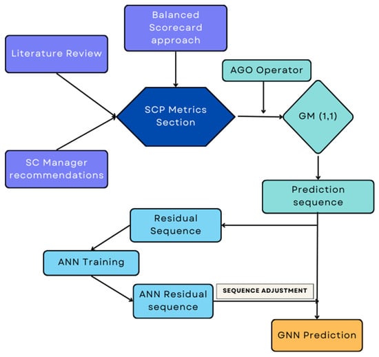
Figure 1.
Flowchart of the overall process.
3.1. GST
GST is common across numerous fields when working with uncertain, partial, and small datasets [37,38,39]. The idea behind the name is that unknown information is black while known information is white; thus, in cases where only partial information is available, the information can be viewed as grey. It addresses the high degree of uncertainty through generation, excavation, and extraction. This systematic treatment of data enables researchers to account for the inherent properties of data and effectively describe system behaviors.
The GST-based prediction model is denoted as GM (), where ‘GM’ stands for grey model, ‘’ represents the order of the differential equation, and ‘’ represents the number of variables. Therefore, GM (1,1) is referred to as the ‘grey first-order one-variable model’. While numerous variations of the model have been developed by researchers for time-series prediction, GM (1, 1) is the most widely used version due to its low complexity and high accuracy. It is worth noting that, before applying the prediction model, the source data must be pre-processed to reduce noise and mitigate the impacts of any undesirable factors hindering the observation of the true system behavior. Hence, we apply some sequence operators to the source data before its incorporation into the prediction model.
3.1.1. Grey Sequence Operators
Buffer Operator:
The buffer operator is denoted by ‘D’. As the raw data sequence is denoted by ‘z’, ‘’ represents the buffer sequence. Two primary types of buffer operators exist, the average weakening buffer operator (AWBO) and the average strengthening buffer operator (ASBO). If the buffered sequence exhibits an increase, decrease, slower fluctuation, or smaller amplitude fluctuation compared to the original sequence z, then D is classified as a weakening operator. Let the original sequence of observed data be z, such that:
then:
where:
Note that, regardless of whether z is a monotonic, increasing, decreasing, or fluctuating sequence, D is always considered an AWBO.
For a second-order weakening operator :
where:
Note that D2 is consistently a second-order weakening buffer operator, irrespective of whether z is a monotonic, increasing, decreasing, or fluctuating sequence.
On the other hand, if the buffered sequence demonstrates a faster increase, decrease, fluctuation, or a larger amplitude fluctuation compared to the original sequence , then is termed as a strengthening operator.
For the original sequence :
and:
where D is called an ASBO, defined as follows:
Average Operator:
Complex system behavior often results in the data sequence missing entries, making it an inaccurate representation of the system. If abnormal entities are removed from the source data, blank entries are created. The missing entries must be filled in from available data to construct a new sequence. Let the original sequence of observed data be z, such that:
where is the preceding term and is the succeeding term. As is the new information for any , represents old information. As the sequence has a blank entry at location , denoted as , the entry is the preceding boundary and is the succeeding boundary. is then an internal point of the interval [, ].
where the new value is generated using new and old information under the generation coefficient . When the generation of is weighted more toward the new information than to the old information; when , it is weighted more toward the old information than to the new information. If , the numerical value denoted as is generated impartially and is identified as the mean generation operation utilizing the non-adjacent neighbor. Typically, such an operation is utilized in situations where determining the impact of both new and old information on the missing value poses a challenge.
Quasi-Smoothness Sequence and Stepwise Ratio Operator:
The fundamental concept behind quasi-smoothness and the stepwise ratio is to assess the stability of variability in the source data points. The greater the stability, the smaller the smoothness ratio . The dataset must be pre-checked for certain conditions before its use in the development of a grey model. If the data sequence is z (Equation (1)), such that:
Then the smoothness ratio is:
In addition, the sequence will be termed a quasi-smooth sequence if the following conditions are met:
In some cases, the first and/or last data entries may be missing, inhibiting the use of the adjacent neighbor mean generation operation. For such cases, we must employ stepwise ratios.
For sequence z (Equation (1)):
If the missing entries are and , then the missing entries should be generated using stepwise ratios of z.
Accumulator Operator (AGO) and Inverse Accumulator Operator (IAGO):
AGO is a process that is used to whitenize a grey process. The quasi-smooth non-negative sequence that AGO generates is likely to show some degree of exponential growth with a dampened variability and randomness. Let the original sequence of observed data be z, such that:
Then:
Where:
In this case, D is known as an accumulating operator of z and is denoted by 1-AGO. If the ‘accumulating operator’ is applied to the data y times, we obtain the following:
where:
In this case, Dy can be denoted as y-AGO.
The IAGO is the opposite of AGO. It reverses the effect of the accumulation process and recovers the data. For the original sequence z (Equation (1)):
then:
where:
D, here, is called an IAGO of z and is denoted by 1-IAGO. This inverse operation on a sequence is also denoted by If the IAGO D is applied y times, then:
where:
3.1.2. Grey Sequence Generation: GM (1,1)
Step 1: Establishing the Original Data Sequence
Having applied the buffer operators, we have established the new sequence z. Let the sequence of source data following buffer operation be , such that:
Step 2: Generating the First-Order Accumulated Generator Operator (1-AGO)
This step of the operation is crucial, as its application decreases randomness/noise during model fitting. The resulting data are a monotonously increasing sequence that satisfies the solution of the first-order differential equation (DE). This allows for an approximate representation of the 1-AGO information based on the solution curve generated from the DE. We must generate the 1-AGO sequence based on .
Step 3: Checking Quasi-Smoothness and Quasi-Index Pattern
We must test the quasi-smoothness of and the quasi-index pattern of . This step is particularly important, as satisfying these conditions facilitates the use of the sequences for building a grey model. The quasi-smoothness test of the sequence is done via the smoothness test ratio. For the sequence , the smoothness ratio () is obtained as follows:
or
The sequence is considered to be a quasi-smooth sequence if smoothness ratio () satisfies Equations (10)–(12). The application of the AGO gives , which must satisfy the quasi-index test before its involvement in the development of a grey model. The quasi-indexed pattern of sequence is tested using the following equation:
Assuming the buffered sequence is a quasi-smooth sequence, for the generated sequence , if , then satisfies the law of quasi-index patterning.
Step 4: Constructing the Mean Generated Sequence/Background Value Sequence
Traditionally, the mean generated sequence (or background value sequence) is used in the differential equation rather than , referred to as an even grey model (EGM). This is because the combination of and does not fulfill the requirement for a flat projection relationship. As the time-series sequence comprises discrete points, it includes boundary points instead of internal points; it is empty between those boundary points. Note that the inner points are derived using the adjacent boundaries from left and right to create a sequence called the mean generated sequence or the background value sequence. The background value sequence is obtained via the following equation:
where and the ‘generating coefficient’ α is usually chosen as 0.5.
Step 5: Developing and Solving the First-Order Differential Equation
We then form the grey differential equation of GM (1,1).
where ‘’ is the developing coefficient and ‘’ is the grey controlled variable. The relevant differential equation (whitenization equation) is as follows:
To estimate the parameters ‘’ and ‘’, we form a matrix such that .
Where:
Then, using the method of minimal squares, we estimate ‘’ and ‘’ as follows:
where:
Step 6: Solving the Whitening Equation
By substituting the values of ‘’ and ‘’ in the grey differential equation, we can achieve a solution for the whitening equation. The resulting sequence is a time-response sequence :
and:
Step 7: Generation of Prediction Sequence
From the sequence of , the prediction sequence is recovered by an IAGO on to obtain the predictive sequence , as follows:
where:
3.2. Artificial Neural Network (ANN)
ANNs mimic the learning properties of a human brain through non-linear information processing via large-scale parallel computing. They can constantly self-learn and make adjustments to conform to the data pattern. They can memorize information, optimize information, reason, and adapt. Hence, ANNs have many applications, including pattern recognition, change prediction, decision optimization, and process enhancement. According to [17], ANNs read datasets in the input node, and certain patterns are used to distribute stored information. The advantage of ANNs over mathematical models is that they do not require precise formulations of physical relationships—they only need output data. They have a simple structure and perform well in the prediction of non-linear systems. A major limitation of ANNs is that they require large datasets for proper training; additionally, factors like slow convergence and prolonged training may result in sub-optimal results. It is also worth noting that the proper determination of the neuron number in ANNs’ implicit layer is undefined in the literature. Thus, iterative decision-making may affect networks’ overall accuracy. Furthermore, ANNs can be greatly affected by randomness, especially if the sample size is limited.
Each ANN consists of input, output, and implicit layers. Each layer consists of multiple processing units called nodes. The nodes are connected across layers via numeric weights that can be modified during the learning phase. The most common ANN is the feed-forward back-propagation neural network (BPNN). Learning samples are provided during the network’s training phase; the samples are used to generate output using an initial weight at the nodes. If the generated output is beyond a predefined acceptance level, the error between the output and the target output is propagated backward through its original route. It diverges from the error-performance function gradient, employing an optimized gradient descent algorithm to iteratively adjust network weights and thresholds until the network output aligns with the target output at the desired accuracy level. Figure 2 is a basic ANN diagram.
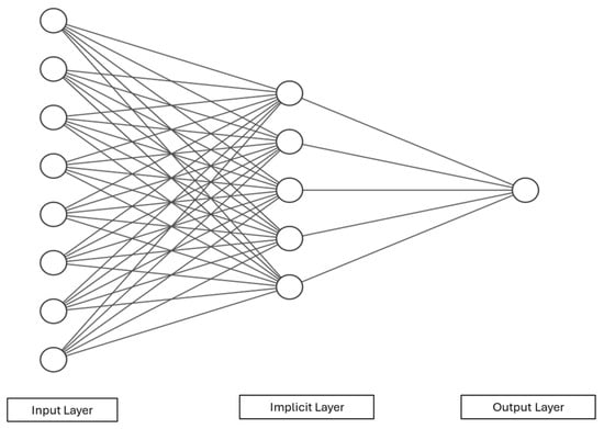
Figure 2.
Artificial neural network.
In Figure 2, let the input layer be the independent inputs to the input layer of the BPNN. The output layer generates the output Layers between the input and output layers are called hidden layers (or hidden layers). The number of implicit layers varies by system complexity. While the number of implicit layers is not predefined by any rule, a single layer is typically chosen for simplicity. However, adding multiple implicit layers can improve network training at the cost of speed—more implicit layers means more time for training. Connection between layers is achieved by weights— and —where represents the connection between the input and the implicit layer and represents the connection between the implicit layer and the output layer.
Let the number of input nodes and output nodes be n and m, respectively, and the threshold for each node be . The number of nodes in the implicit layer is l. The computational scheme of a typical BPNN abides by the following algorithms.
- (i)
- Forward propagation in BPNN
The output of the implicit layer is generated as follows:
The output of the output layer is generated as follows:
The initial generated output vector is compared to the expected output vector, and a mean square error function is generated, which can be defined as follows:
where represents the components of the expected output vectors.
- (ii)
- Error back-propagation in BPNN
The error function of the BPNN can be obtained by substituting and in :
After deriving the error function concerning the weights and threshold values of the outputs, we can obtain the error of the output node.
In the output layer node, the weights and threshold adjustment are as follows:
In Equations (35) and (36), is defined as the BPNN’s learning rate. The adjustment algorithm of the weights and threshold values is very significant in training and affects the forecasting accuracy.
While several algorithms are available for network training, the Levenberg–Marquardt algorithm is the most common choice among researchers. The LM algorithm is generally a non-linear training algorithm based on the combination of the gradient descent method and the quasi-Newton method. It generally enhances the network’s convergence speed and overall performance. The LN algorithm behaves as the gradient descent method when the initial solution is far from the target solution. This ensures convergence in the iterations. However, as the solution closes in on the target solution, we apply the quasi-Newton method. Additionally, the network weights are adjusted alongside the combination of the two methods, which, in effect, allows the network to efficiently converge at an increased speed.
3.3. Proposed Model
This article proposes the construction of a grey-based neural network model that pairs GM (1,1) with ANN. This proposed model simultaneously boasts the low data requirements of grey models and the non-linear mapping capabilities of ANNs. Figure 3 details the steps involved in the model’s formulation.
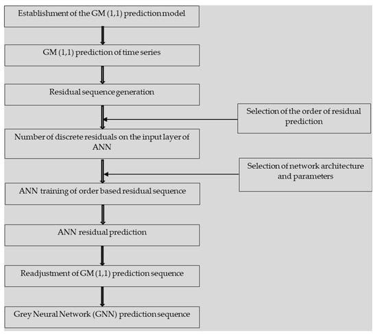
Figure 3.
GNN model.
Initially, we use GM (1,1) for a prediction based on the original data sequence. Based on the generated output, the residual sequence can be generated through a comparison with the predicted data. We then use the residual sequence , generated in line with Equation (37), for ANN prediction.
The architecture of the ANN is determined based on the characteristics of the residual sequence. The order of prediction is a crucial factor in ANN training. Although there is no predefined rule for setting prediction order, researchers should maximize the number of different sets of input. A prediction-order decision can be made based on an iterative process. If the order of prediction is then the inputs selected would be for predicting the kth period, while the outputs selected would be , where . The ordered residual sequence is then used to train a BPNN. Thus, the training value obtained through the network can predict the error in the predetermined order. This predicted residual sequence () can then be used to adjust the initial prediction from the GM (1,1) model to form the final prediction sequence, as per Equation (38).
3.4. Proposed Model
Table 1 represents the mean relative error requirements for a varying accuracy scale. The mean relative error () and mean relative accuracy are calculated based on Equations (39) and (40).
where and n represent the number of data points in the original sequence.

Table 1.
Accuracy scale for model testing.
4. Case Analysis
To validate the model, numerical examples were conducted with three Bangladeshi apparel-manufacturing companies, specializing in casual wear and undergarments. The companies, while undisclosed for confidentiality reasons, are well-established members of the Bangladesh Garment Manufacturers and Exporters Association, differing in their annual turnover, production scale, and volume.
Company 1, established in 2000 with an initial investment of $600 million, boasts an annual turnover of approximately $180 million. With 11,000 employees, it exports high-quality garments to European brands, holding the highest total export value in Bangladesh for the past 11 years. Its representative SCP indicators include its market share, profitability, turnover ratios, response time, stock turnover, information sharing, R&D, and delivery performance.
Company 2, a leading Chinese apparel exporter in Bangladesh, operates modern machinery and vertically integrated facilities with around 8000 workers. The selected indicators for this company include its turnover time, profitability, response time, information sharing, and delivery performance, omitting consumer-related attributes for confidentiality.
Company 3, founded in 1997, exhibits the lowest annual turnover among the three. It exports garments to European and North American fashion brands, focusing on customer satisfaction, turnover ratios, waste management, profit increment, delivery performance, and flexibility.
Despite their differences, all of these companies utilize internal management to navigate market uncertainties and strategize for a competitive advantage. A reliable prediction model accommodating uncertainty would aid in predicting SCP, thereby enhancing the supply chain performance and informing strategic decisions.
4.1. Application of the Balanced Scorecard
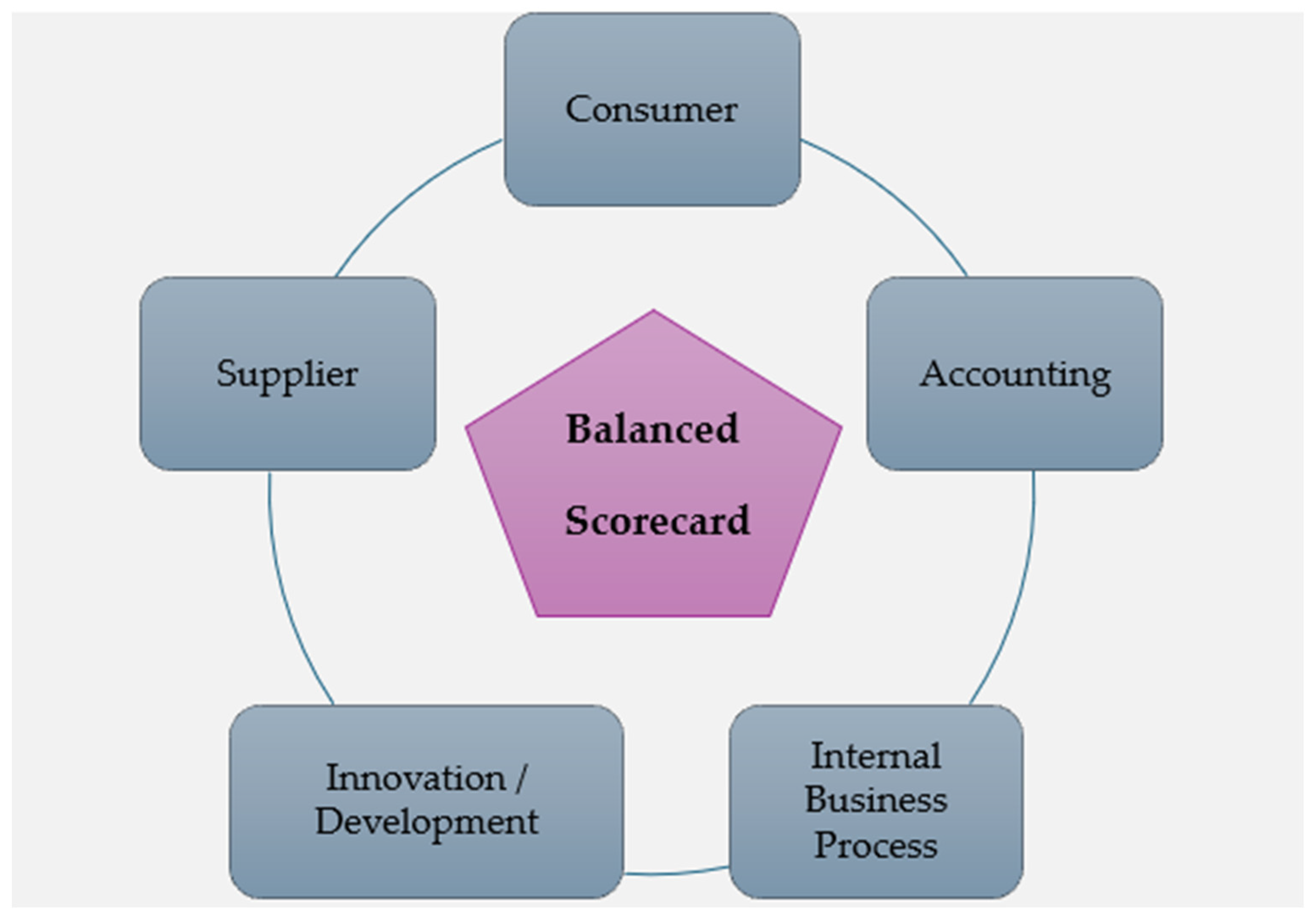
We adopted the BSC approach to select indicators for our cases. Considering both our literature review and company expertise, this article supplements the traditional components with a supplier component, as shown in Figure 4. This can be justified, as there is a great dependency on the outsourcing of certain components in the production process. It expands across numerous SC stages.
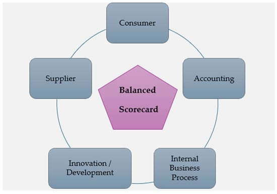
Figure 4.
Balanced scorecard approach.
KPIs across three broad categories have been selected based on applicability, availability, literature review considerations, and company feedback. The use of these attributes for the representation of SCs has been suggested by academic experts. The attributes are as follows: accounting, supplier, internal business process, innovation, development, and customer satisfaction. The KPI lists for the three companies are displayed in Table 2, Table 3 and Table 4.
Table 2.
SCM KPIs of Company 1.
Table 3.
SCM KPIs of Company 2.
Table 4.
SCM KPIs of Company 3.
A brief explanation of each of the KPIs used in the model is given below.
- ▪
- Market share: Percentage of total sales in an industry generated by the company, as recorded by the company;
- ▪
- Profitability: The difference between the revenue and costs, as recorded by the company;
- ▪
- Capital turnover rate: Represents the capital turnover rate as recorded by the company;
- ▪
- Cash turnover time: Turnover time in days; the data collected were scaled down by an unknown factor for confidentiality;
- ▪
- SC response time: The time the SC takes, in days, to adjust its operations in line with sudden market shifts, as recorded by the company;
- ▪
- Stock market cash availability: Cash, in Bangladeshi taka (BDT), that is available through the stock market; the data collected were scaled down by an unknown factor for confidentiality;
- ▪
- Information sharing: Rate of information sharing between SC stages; both qualitative and numerical values collected on a 0–10 scale based on manager feedback (higher values represent better performance);
- ▪
- New product period: Number of days required from order receipt to product provision;
- ▪
- Rate of on-time delivery: Percentage of successful product provisions;
- ▪
- Flexibility: Ability of the SC to buffer supplier uncertainty; both qualitative and numerical values collected on a 0–10 scale based on manager feedback (higher values represent better performance);
- ▪
- Customer satisfaction: Satisfaction level of buyers after receiving the company’s product;
- ▪
- Waste rate: Proportion of products that failed to meet order specifications and requirements;
- ▪
- Profit increment rate: The company’s development capability, based on incremental profits generated by delivery completion.
Although the selected indicators vary among the three different case studies, the construction of the GNN model is similar for all of these cases. Hence, we only show the modeling process in detail for Company 1. However, we report the accuracy of all of the case studies in the results section. The relevant tables for Company 2 and Company 3 can be found in Appendix A.
4.2. Construction of the GM (1,1) Model
The construction of the GM (1,1) model (as discussed in Section 3.1) was conducted via the following steps:
- ▪
- Step 1: To establish the original data sequence, take the collected KPI data (Table 5, Table 6 and Table 7 for Company 1, Company 2, and Company 3, respectively) as input for ;
Table 5. SCM KPIs from Company 1.
Table 6. SCM KPIs from Company 2.
Table 7. SCM KPIs from Company 3.
- ▪
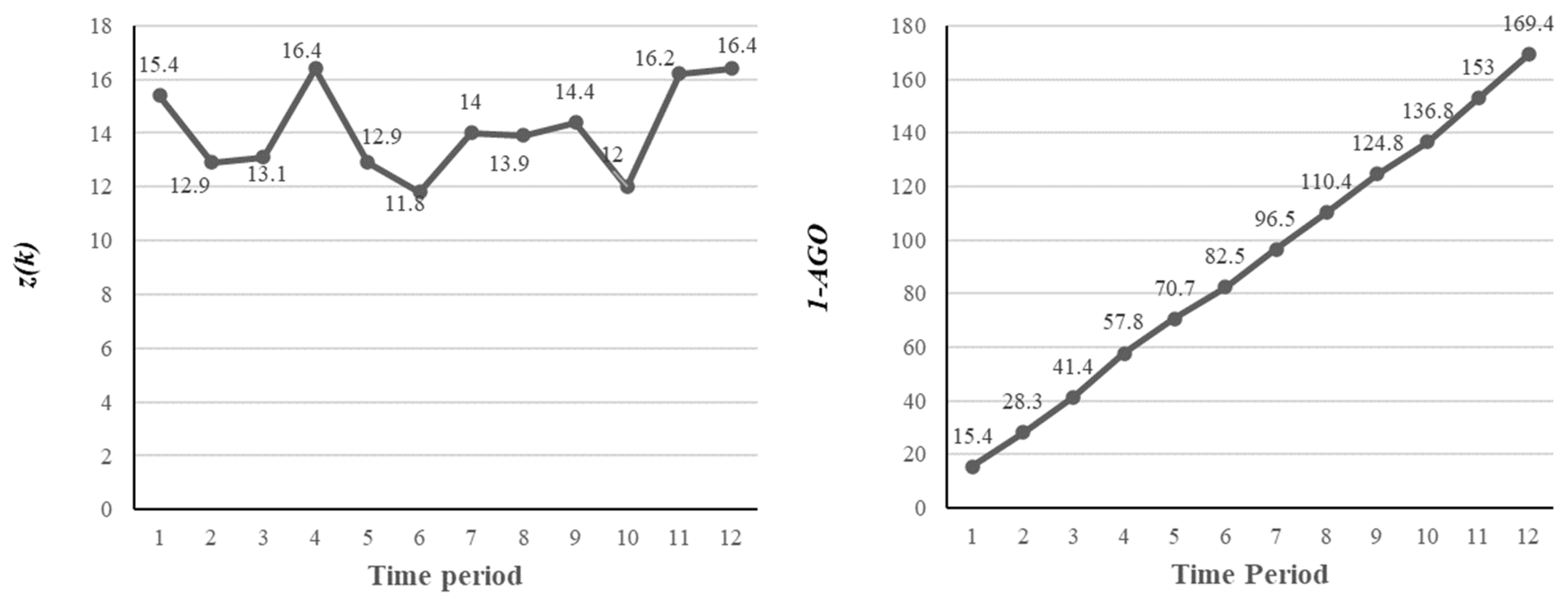
- Step 2: Establish the first-order accumulated generator operator (1-AGO) as presented in Table 8 for company 1.
Table 8. values for Company 1.
A plot of and of I11 is shown in Figure 5. The reduced randomness in the 1-AGO sequence is a crucial factor in the prediction accuracy of the GM (1,1) model.
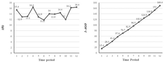
Figure 5.
Representation of the data pattern of I11.
Before step three, the sequence must be tested for the quasi-smoothness of and the quasi-index pattern of . This step is particularly important, as satisfying these conditions allows for the use of sequences in the development of the grey model.
- ▪
- Step 3: Obtain the mean generated sequence/background value sequence (Table 9);
Table 9. Mean generated sequence of the KPIs for Company 1.
- ▪
- Step 4: Use the mean generated sequence and the original sequence to construct the grey differential equation. The differential equation can be solved by forming a matrix, and is used to estimate the parameters developing coefficient (a) and the grey controlled variable/grey input (Table 10);
Table 10. Estimation of developing coefficient and grey input for Company 1.
- ▪
- Step 5: Use the values of developing coefficient (a) and grey input (b) to achieve the solution for the whitening equation, as per Equations (27) and (28). The prediction sequence is () (Table 11).
Table 11. Prediction sequence, , for Company 1.
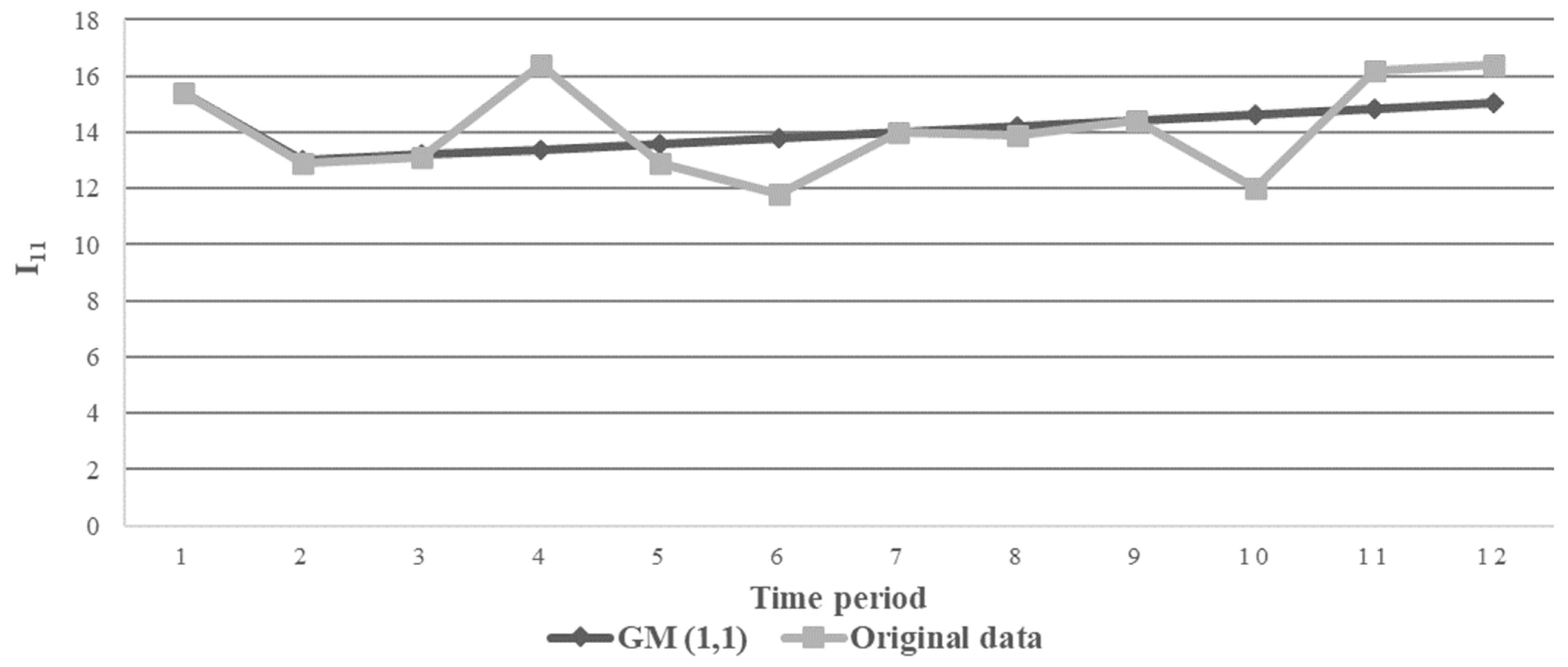
Figure 6 shows the GM (1,1)’s predicted sequence against the original data sequence for KPI I11 of Company 1.

Figure 6.
Illustration of GM (1,1) prediction and original sequence of I11.
4.3. Construction of the Grey-Based Neural Network (GNN) Model
The development of the GNN involves two stages. First, the ANN is configured based on the data pattern and the desired prediction order. The ANN is configured as a 2-5-1 system (i.e., the input layer consists of two neurons; the implicit layer consists of five neurons; and the output layer consists of one neuron). We set up a two-node input layer on account of the desired prediction order of 2. This allows for a large number of distinct dataset combinations, ensuring better training conditions. The ANN performance depends on the choice of prediction order. A higher prediction order reduces overfitting; however, considering the available data, a prediction order of 2 is the best fit. There is no predefined rule for determining the number of neurons in the implicit layer despite the choice being of extreme significance. A lower number inhibits the network’s capability in terms of the sample input’s identity, training, and fault tolerance; a higher number increases the number of iterations necessary and, in turn, hinders both the completion time and accuracy. For the network, the transfer function used is Tansig. While training, the function is Trainlm (LM training algorithm); while learning, the function is Learngdm (Gradient descent rule). The performance function used is the mean squared error (MSE). The maximum epoch is set at 1000.
After obtaining the residual sequence from the initial GM (1,1) predictions, the next step involves preprocessing, data cleaning, and splitting the data for further analysis and model training. First, missing values and outliers are identified and addressed through imputation (mean value of training set), as they can distort the analysis and model performance. Following preprocessing, the data should be split into training (70%), validation (15%), and testing (15%) sets to evaluate model performance effectively. The training set is used to train the neural network on historical data, while the validation set is employed to tune hyperparameters and prevent overfitting. Finally, the testing set, which remains unseen by the model during training, is used to report the model’s performance.
We use the residual sequence from GM (1,1) to train the ANN and, in turn, make predictions to form the predicted error sequence, . In the second stage of constructing the GNN, we incorporate the predicted error sequence into the original prediction sequence of GM (1,1) to generate the GNN prediction sequence, (see Table 12).
Table 12.
GNN prediction sequence, , for Company 1.
Figure 7 shows the GNN predicted sequence against the original data sequence for KPI I11 of Company 1.
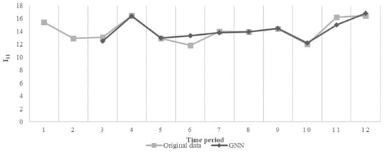
Figure 7.
Illustration of GNN prediction and original sequence for I11.
4.4. Findings and Discussion
There are no pre-defined rules regarding the optimal number of neurons in the implicit layer; we set the number at five based on iterations on the network. The output being a single data point on the residual sequence resulted in a one-node output selection. We finalized all other network parameters on a trial-and-error basis. We adjusted the predicted residual sequence stemming from network training in line with the initial GM (1,1) prediction sequence to find a GNN prediction sequence.
Table 13 compares the mean relative error and mean relative accuracy between GM (1,1) and the GNN for Company 1. Six of the KPIs exhibit changes in accuracy, while all of the KPIs exhibit a decrease in both their mean relative accuracy and mean relative error. The bar chart above illustrates the changes in the mean relative error. Table 14 lists the percentage change in the mean relative error between GM (1,1) and the GNN. We can observe a reduction in the mean relative error for all of the KPIs. The highest reduction was one of 70.54% for KPI 10; the lowest reduction was one of 0.23% for KPI 5.
Table 13.
GM (1,1) and GNN mean relative accuracy for Company 1.
Table 14.
Percentage change in mean relative error for Company 1.
For Company 2, four of the five KPIs have shifts in their mean relative accuracy, though the change was not significant for one of them, as depicted in Table 15. Table 16 illustrates the percentage change in the mean relative error for the KPIs of Company 2. All five saw significant reductions. The highest reduction was one of 77.09% for KPI 1 (77.09%); the lowest reduction was one of 50.51% for KPI 3 (50.51%).
Table 15.
GM (1,1) and GNN mean relative accuracy for Company 2.
Table 16.
Percentage change in mean relative error for Company 2.
For Company 3, all of the indicators improved by one level in the prediction accuracy scale, though KPIs 4 and 5 failed to be within an acceptable range using GM (1,1). However, the GNN reduced the errors significantly, bringing it within an acceptable range (Table 17). Table 18 shows the percentage change in the mean relative error for the KPIs of Company 3. The highest reduction was one of 72.94%; the lowest reduction was one of 22.05% for KPI 1.
Table 17.
GM (1,1) and GNN mean relative accuracy for Company 3.
Table 18.
Percentage change in mean relative error for Company 3.
The changes in all of the KPIs across all three companies are plotted in Figure 8. The highest reduction was one of 77.09% for KPI 1 of Company 2 (I21); the lowest reduction was one of 0.23% for KPI 5 of Company 1 (I15).
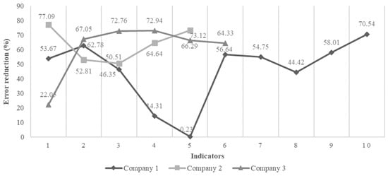
Figure 8.
Percentage reduction in error for GNN prediction.
In the case of I15, the GM (1,1) attained a good fit (level 2). This could be attributed to the stable changes in the source sequence of the indicator. Although the GNN performed slightly better for I15, further improvement is inhibited by the prediction order, which is largely based on the availability of distinct data combinations. Through the inclusion of new datasets in the source sequence, we can achieve a prediction order that is more optimized, resulting in a greater performance. Overall, the mean relative accuracy increased from the GM (1,1) model to the GNN. This indicates that the GNN is a reliable, robust, and efficient model for time-series prediction. It has the potential to aid SC managers in developing strategies and policies to stay ahead of their competition.
5. Conclusions
Drawing inspiration from the categorization of SCP metrics in the existing literature, this study examines five dimensions of SCP metrics across three cases. These dimensions include the consumer attribute, accounting attribute, internal business process attribute, innovation/development attribute, and supplier attribute. In this context, a total of 21 KPIs from three different apparel manufacturing companies in Bangladesh are selected for case analysis.
The hybrid GNN model was implemented for SCP prediction and benchmarked against the traditional GM (1,1) model. Although GM (1,1) has been able to achieve acceptable results in most of the time-series sequence, except for two indicators from Company 3, the application of the GNN has been able to reduce the prediction error for all the KPIs. The hybrid model sufficiently utilizes the attributes of the grey system model, requiring fewer data and features of a non-linear map of the neural network. The proposed model reduced the MRE for all indicators considered. For company 1, the range of percentage reduction in MRE is 70.54–0.23%, for Company 2, the range is 77.09–50.51%, and for Company 3, the range is 72.94–22.01%. This performance improvement illustrates the effectiveness of the GNN model as a prediction model and outperforms the traditional GM (1,1) by overcoming the associated constraints. The proposed methodology of KPI prediction in this paper can aid SC managers in the evaluation of SCP and, in turn, in the maintenance of competitive advantage and economic sustainability.
6. Limitations and Further Research
The inherent nature of the source data in our case studies remains unknown, leading us to overlook buffer operators in our analysis. Exploring the source data distribution could provide valuable insights for future modeling efforts. Moreover, our choice of prediction order was constrained by data limitations. Increasing the sample size could mitigate this issue and enhance the overall performance of our GNN model. Furthermore, a deeper understanding of the source data’s intrinsic characteristics would facilitate noise reduction. By discerning the growth tendencies of our data, we could implement strengthening and weakening buffer operators to refine the predictive capabilities of the GNN model. Looking ahead, with a sufficiently large data source, the development of machine learning algorithms for future time-series predictions becomes viable. Decision tree regression and random forest regression are established methods in scenarios of robust data availability, and the incorporation of gradient-boosted trees would further elevate the model’s predictive prowess.
Author Contributions
Conceptualisation, S.M.A., A.U.R., G.K. and S.K.P.; methodology, S.M.A., A.U.R., G.K. and S.K.P.; software, S.M.A. and A.U.R.; validation, S.M.A., A.U.R. and G.K.; formal analysis, A.U.R.; investigation, S.M.A., A.U.R. and G.K.; resources, S.M.A. and G.K.; data curation, A.U.R.; writing—original draft preparation, S.M.A. and A.U.R.; writing—review and editing, S.M.A., G.K. and S.K.P.; visualisation, S.M.A. and A.U.R.; supervision, S.M.A.; project administration, S.M.A. All authors have read and agreed to the published version of the manuscript.
Funding
This research received no external funding.
Institutional Review Board Statement
Not applicable.
Informed Consent Statement
Not applicable.
Data Availability Statement
Data used are embedded in this article.
Acknowledgments
The authors are grateful to the experts for supporting this project.
Conflicts of Interest
The authors declare no conflicts of interest.
Appendix A
Table A1.
values for Company 2.
Table A1.
values for Company 2.
| Period (Month) | Accounting Attribute | Internal Business Process Attribute | Innovation & Development Attribute | Supplier Attribute | |
|---|---|---|---|---|---|
| I21 | I22 | I23 | I24 | I25 | |
| 1 | 91 | 53.6 | 91 | 8 | 97 |
| 2 | 201 | 114.6 | 180 | 17 | 196 |
| 3 | 307 | 172.9 | 270 | 26 | 292 |
| 4 | 397 | 220.5 | 356 | 36 | 387 |
| 5 | 498 | 271.7 | 441 | 46 | 485 |
| 6 | 604 | 325.4 | 529 | 55 | 581 |
| 7 | 694 | 375.5 | 615 | 64 | 680 |
| 8 | 797 | 427.4 | 703 | 74 | 777 |
| 9 | 882 | 488.2 | 793 | 84 | 877 |
| 10 | 985 | 534.4 | 885 | 92 | 973 |
| 11 | 1105 | 595 | 970 | 102 | 1068 |
| 12 | 1218 | 645.3 | 1062 | 112 | 1168 |
Table A2.
values for Company 3.
Table A2.
values for Company 3.
| Period (Month) | Customer Attribute | Accounting Attribute | Internal Business Process Attribute | Innovation & Development Attribute | Supplier Attribute | |
|---|---|---|---|---|---|---|
| I31 | I32 | I33 | I34 | I35 | I35 | |
| 1 | 4 | 0.387 | 0.059 | 0.31 | 9 | 4 |
| 2 | 8 | 0.733 | 0.13 | 0.581 | 19 | 10 |
| 3 | 11 | 1.14 | 0.209 | 1.341 | 26 | 16 |
| 4 | 15 | 1.572 | 0.271 | 1.551 | 31 | 22 |
| 5 | 19 | 1.97 | 0.352 | 1.791 | 40 | 30 |
| 6 | 22 | 2.276 | 0.425 | 2.152 | 50 | 38 |
| 7 | 25 | 2.657 | 0.516 | 2.722 | 56 | 44 |
| 8 | 29 | 3.033 | 0.583 | 3.182 | 66 | 52 |
| 9 | 32 | 3.525 | 0.667 | 3.348 | 71 | 60 |
| 10 | 36 | 3.851 | 0.735 | 3.742 | 81 | 67 |
| 11 | 40 | 4.204 | 0.812 | 4.271 | 89 | 76 |
| 12 | 44 | 4.571 | 0.899 | 4.761 | 98 | 84 |
Table A3.
Estimation of developing coefficient and grey input for Company 2.
Table A3.
Estimation of developing coefficient and grey input for Company 2.
| Indicators | Developing Coefficient (a) | Grey Input (b) |
|---|---|---|
| I21 | −0.0070 | 97.9030 |
| I22 | 0.0054 | 55.6950 |
| I23 | −0.0023 | 86.8990 |
| I24 | −0.0038 | 9.2251 |
| I25 | −0.0008 | 96.8315 |
Table A4.
Estimation of developing coefficient and grey input for Company 3.
Table A4.
Estimation of developing coefficient and grey input for Company 3.
| Indicators | Developing Coefficient (a) | Grey Input (b) |
|---|---|---|
| I31 | −0.0078 | 3.4497 |
| I32 | 0.0040 | 0.3903 |
| I33 | −0.0107 | 0.0713 |
| I34 | −0.0161 | 0.3646 |
| I35 | −0.0070 | 7.7193 |
| I36 | −0.0306 | 5.9919 |
Table A5.
Prediction sequence, , for Company 2.
Table A5.
Prediction sequence, , for Company 2.
| Period (k) | |||||
|---|---|---|---|---|---|
| I21 | I22 | I23 | I24 | I25 | |
| 1 | 91 | 53.6 | 91 | 8 | 97 |
| 2 | 98.88957 | 55.25588 | 87.22094 | 9.273782 | 96.9541 |
| 3 | 99.58696 | 54.95801 | 87.42977 | 9.309516 | 97.0358 |
| 4 | 100.2893 | 54.66175 | 87.6391 | 9.345388 | 97.11757 |
| 5 | 100.9965 | 54.36708 | 87.84894 | 9.381398 | 97.19941 |
| 6 | 101.7088 | 54.074 | 88.05927 | 9.417547 | 97.28131 |
| 7 | 102.426 | 53.7825 | 88.27011 | 9.453835 | 97.36328 |
| 8 | 103.1484 | 53.49258 | 88.48146 | 9.490262 | 97.44533 |
| 9 | 103.8758 | 53.20421 | 88.69331 | 9.526831 | 97.52744 |
| 10 | 104.6083 | 52.9174 | 88.90566 | 9.56354 | 97.60962 |
| 11 | 105.346 | 52.63214 | 89.11853 | 9.60039 | 97.69187 |
| 12 | 106.089 | 52.34841 | 89.3319 | 9.637383 | 97.77419 |
Table A6.
Prediction sequence, , for Company 3.
Table A6.
Prediction sequence, , for Company 3.
| Period (k) | ||||||
|---|---|---|---|---|---|---|
| I31 | I32 | I33 | I34 | I35 | I35 | |
| 1 | 4 | 0.387 | 0.059 | 0.31 | 9 | 4 |
| 2 | 3.49494869 | 0.392669 | 0.072331 | 0.37267 | 7.809888 | 6.209556 |
| 3 | 3.52254206 | 0.395769 | 0.073112 | 0.378741 | 7.864875 | 6.403104 |
| 4 | 3.55035329 | 0.398894 | 0.073901 | 0.38491 | 7.920249 | 6.602685 |
| 5 | 3.5783841 | 0.402043 | 0.074698 | 0.39118 | 7.976013 | 6.808486 |
| 6 | 3.60663621 | 0.405217 | 0.075504 | 0.397551 | 8.03217 | 7.020702 |
| 7 | 3.63511138 | 0.408417 | 0.076319 | 0.404027 | 8.088722 | 7.239533 |
| 8 | 3.66381137 | 0.411641 | 0.077142 | 0.410608 | 8.145672 | 7.465184 |
| 9 | 3.69273795 | 0.414891 | 0.077975 | 0.417297 | 8.203023 | 7.697869 |
| 10 | 3.72189291 | 0.418167 | 0.078816 | 0.424094 | 8.260778 | 7.937806 |
| 11 | 3.75127805 | 0.421468 | 0.079666 | 0.431002 | 8.31894 | 8.185223 |
| 12 | 3.7808952 | 0.424796 | 0.080526 | 0.438023 | 8.377511 | 8.440351 |
Table A7.
GNN prediction sequence, , for Company 2.
Table A7.
GNN prediction sequence, , for Company 2.
| Period (k) | |||||
|---|---|---|---|---|---|
| I21 | I22 | I23 | I24 | I25 | |
| 1 | - | - | - | - | - |
| 2 | - | - | - | - | - |
| 3 | 111.76 | 59.431 | 89.976 | 9.175 | 96.569 |
| 4 | 92.844 | 47.60 | 85.906 | 9.565 | 96.209 |
| 5 | 101 | 48.569 | 86.601 | 10.001 | 98.134 |
| 6 | 106 | 57.655 | 87.579 | 9.00 | 95.972 |
| 7 | 90 | 51.509 | 85.397 | 8.00 | 98.974 |
| 8 | 103 | 52.682 | 88.012 | 9.808 | 97.545 |
| 9 | 85.0004 | 56.473 | 89.995 | 10.001 | 99.038 |
| 10 | 104.354 | 46.142 | 91.940 | 8.007 | 96.358 |
| 11 | 119.999 | 60.577 | 85.084 | 9.990 | 95.024 |
| 12 | 120.727 | 45.287 | 85.272 | 9.999 | 99.759 |
Table A8.
GNN prediction sequence, , for Company 3.
Table A8.
GNN prediction sequence, , for Company 3.
| Period (k) | ||||||
|---|---|---|---|---|---|---|
| I31 | I32 | I33 | I34 | I35 | I35 | |
| 1 | - | - | - | - | - | - |
| 2 | - | - | - | - | - | - |
| 3 | 3.258 | 0.390 | 0.078 | 0.621 | 6.984 | 6.001 |
| 4 | 3.467 | 0.436 | 0.062 | 0.209 | 7.046 | 6.758 |
| 5 | 3.449 | 0.408 | 0.079 | 0.139 | 9.943 | 7.397 |
| 6 | 3.034 | 0.324 | 0.071 | 0.360 | 9.846 | 7.998 |
References
- Balfaqih, H.; Nopiah, Z.M.; Saibani, N.; Al-Nory, M.T. Review of supply chain performance measurement systems: 1998–2015. Comput. Ind. 2016, 82, 135–150. [Google Scholar] [CrossRef]
- Baryannis, G.; Dani, S.; Antoniou, G. Predicting supply chain risks using machine learning: The trade-off between performance and interpretability. Futur. Gener. Comput. Syst. 2019, 101, 993–1004. [Google Scholar] [CrossRef]
- Mangla, S.K.; Kusi-Sarpong, S.; Luthra, S.; Bai, C.; Jakhar, S.K.; Khan, S.A. Operational excellence for improving sustainable supply chain performance. Resour. Conserv. Recycl. 2020, 162, 105025. [Google Scholar] [CrossRef]
- Taelman, S.; Sanjuan-Delmás, D.; Tonini, D.; Dewulf, J. An operational framework for sustainability assessment including local to global impacts: Focus on waste management systems. Resour. Conserv. Recycl. X 2020, 162, 104964. [Google Scholar] [CrossRef]
- Bag, S.; Wood, L.C.; Xu, L.; Dhamija, P.; Kayikci, Y. Big data analytics as an operational excellence approach to enhance sustainable supply chain performance. Resour. Conserv. Recycl. 2019, 153, 104559. [Google Scholar] [CrossRef]
- Rahman, A.U.; Zahura, M.T. A Grey Approach for the Prediction of Supply Chain Demand. Am. J. Ind. Eng. 2018, 5, 25–30. [Google Scholar] [CrossRef]
- Frederico, G.F.; Garza-Reyes, J.A.; Kumar, A.; Kumar, V. Performance measurement for supply chains in the Industry 4.0 era: A balanced scorecard approach. Int. J. Prod. Perform. Manag. 2020, 70, 789–807. [Google Scholar] [CrossRef]
- Ka, J.M.R.; Ab, N.R.; Lb, K. A review on supply chain performance measurement systems. Procedia Manuf. 2019, 30, 40–47. [Google Scholar] [CrossRef]
- Nouri, F.A.; Nikabadi, M.S.; Olfat, L. Developing the framework of sustainable service supply chain balanced scorecard (SSSC BSC). Int. J. Prod. Perform. Manag. 2019, 68, 148–170. [Google Scholar] [CrossRef]
- Reefke, H.; Trocchi, M. Balanced scorecard for sustainable supply chains: Design and development guidelines. Int. J. Prod. Perform. Manag. 2013, 62, 805–826. [Google Scholar] [CrossRef]
- Bhagwat, R.; Sharma, M.K. Performance measurement of supply chain management: A balanced scorecard approach. Comput. Ind. Eng. 2007, 53, 43–62. [Google Scholar] [CrossRef]
- Huang, C.-K.; Wang, T.; Huang, T.-Y. Initial Evidence on the Impact of Big Data Implementation on Firm Performance. Inf. Syst. Front. 2018, 22, 475–487. [Google Scholar] [CrossRef]
- Zu, X.; Yang, C.; Wang, H.; Wang, Y. An EGR performance evaluation and decision-making approach based on grey theory and grey entropy analysis. PLoS ONE 2018, 13, e0191626. [Google Scholar] [CrossRef]
- Liu, C.; Xie, W.; Lao, T.; Yao, Y.-T.; Zhang, J. Application of a novel grey forecasting model with time power term to predict China′s GDP. Grey Syst. Theory Appl. 2020, 11, 343–357. [Google Scholar] [CrossRef]
- Qu, P. Mobile communication service income prediction method based on grey buffer operator theory. Grey Syst. Theory Appl. 2014, 4, 250–259. [Google Scholar] [CrossRef]
- Sezer, O.B.; Gudelek, M.U.; Ozbayoglu, A.M. Financial time series forecasting with deep learning: A systematic literature review: 2005–2019. Appl. Soft Comput. 2020, 90, 106181. [Google Scholar] [CrossRef]
- Ye, Z.; Kim, M.K. Predicting electricity consumption in a building using an optimized back-propagation and Levenberg–Marquardt back-propagation neural network: Case study of a shopping mall in China. Sustain. Cities Soc. 2018, 42, 176–183. [Google Scholar] [CrossRef]
- Mishra, D.; Gunasekaran, A.; Papadopoulos, T.; Dubey, R. Supply chain performance measures and metrics: A bibliometric study. Benchmark. Int. J. 2018, 25, 932–967. [Google Scholar] [CrossRef]
- Chorfi, Z.; Benabbou, L.; Berrado, A. An integrated performance measurement framework for enhancing public health care supply chains. Supply Chain Forum Int. J. 2018, 19, 191–203. [Google Scholar] [CrossRef]
- Fan, X.; Zhang, S.; Wang, L.; Yang, Y.; Hapeshi, K. An evaluation model of supply chain performances using 5DBSC and LMBP neural network algorithm. J. Bionic Eng. 2013, 10, 383–395. [Google Scholar] [CrossRef]
- Kaplan, R.S.; Norton, D.P. The balanced scorecard: Measures that drive performance. Harv. Bus Rev. 2005, 83, 172. [Google Scholar]
- Chai, J.; Liu, J.N.; Ngai, E.W. Application of decision-making techniques in supplier selection: A systematic review of literature. Expert Syst. Appl. 2013, 40, 3872–3885. [Google Scholar] [CrossRef]
- Trivedi, A.; Rajesh, K. A framework for performance measurement in supply chain using balanced score card method: A case study. Int. J. Recent Trends Mech. Eng. 2013, 4, 20–23. [Google Scholar]
- Xia, D.; Yu, Q.; Gao, Q.; Cheng, G. Sustainable technology selection decision-making model for enterprise in supply chain: Based on a modified strategic balanced scorecard. J. Clean. Prod. 2017, 141, 1337–1348. [Google Scholar] [CrossRef]
- Thanki, S.; Thakkar, J. A quantitative framework for lean and green assessment of supply chain performance. Int. J. Prod. Perform. Manag. 2018, 67, 366–400. [Google Scholar] [CrossRef]
- Agarwal, A.; Shankar, R.; Tiwari, M. Modeling the metrics of lean, agile and leagile supply chain: An ANP-based approach. Eur. J. Oper. Res. 2006, 173, 211–225. [Google Scholar] [CrossRef]
- Lima-Junior, F.R.; Carpinetti, L.C.R. An adaptive network-based fuzzy inference system to supply chain performance evaluation based on SCOR® metrics. Comput. Ind. Eng. 2019, 139, 106191. [Google Scholar] [CrossRef]
- Elrod, C.; Murray, S.; Bande, S. A review of performance metrics for supply chain management. Eng. Manag. J. 2013, 25, 39–50. [Google Scholar] [CrossRef]
- Beamon, B.M. Measuring supply chain performance. Int. J. Oper. Prod. Manag. 1999, 19, 275–292. [Google Scholar] [CrossRef]
- Chen, K. Research and Practice of the Models of Supply Chain Performance in Manufacturing Industry. Ph.D. Thesis, Tianjin University, Tianjin, China, 2009. (In Chinese). [Google Scholar]
- Gunasekaran, A.; Patel, C.; Tirtiroglu, E. Performance measures and metrics in a supply chain environment. Int. J. Oper. Prod. Manag. 2001, 21, 71–87. [Google Scholar] [CrossRef]
- Billah, B.; King, M.L.; Snyder, R.D.; Koehler, A.B. Exponential smoothing model selection for forecasting. Int. J. Forecast. 2006, 22, 239–247. [Google Scholar] [CrossRef]
- Tsaur, R.-C. Forecasting by fuzzy double exponential smoothing model. Int. J. Comput. Math. 2003, 80, 1351–1361. [Google Scholar] [CrossRef]
- Makridakis, S.; Andersen, A.; Carbone, R.; Fildes, R.; Hibon, M.; Lewandowski, R.; Newton, J.; Parzen, E.; Winkler, R. The accuracy of extrapolation (time series) methods: Results of a forecasting competition. J. Forecast. 1982, 1, 111–153. [Google Scholar] [CrossRef]
- Makridakis, S.; Hibon, M. The M3-Competition: Results, conclusions and implications. Int. J. Forecast 2000, 16, 451–476. [Google Scholar] [CrossRef]
- Chan, H.K.; Xu, S.; Qi, X. A comparison of time series methods for forecasting container throughput. Int. J. Logist. Res. Appl. 2018, 22, 294–303. [Google Scholar] [CrossRef]
- Julong, D. Introduction to grey system theory. J. Grey Syst. 1989, 1, 1–24. [Google Scholar]
- Deng, J.-L. Control problems of grey systems. Syst. Contr. Lett. 1982, 1, 288–294. [Google Scholar]
- Liu, S.F.; Yang, Y.; Forrest, J. Grey Data Analysis; Springer: Berlin/Heidelberg, Germany, 2017. [Google Scholar]
- Samvedi, A.; Jain, V. A grey approach for forecasting in a supply chain during intermittentdisruptions. Eng. Appl. Artif. Intell. 2013, 26, 1044–1051. [Google Scholar] [CrossRef]
- Hsu, C.-C.; Chen, C.-Y. Applications of improved grey prediction model for power demand forecasting. Energy Convers. Manag. 2003, 44, 2241–2249. [Google Scholar] [CrossRef]
- Pang, X.; Li, Z.; Tseng, M.-L.; Liu, K.; Tan, K.; Li, H. Electric Vehicle Relay Lifetime Prediction Model Using the Improving Fireworks Algorithm–Grey Neural Network Model. Appl. Sci. 2020, 10, 1940. [Google Scholar] [CrossRef]
- Chen, K.; Laghrouche, S.; Djerdir, A. Degradation prediction of proton exchange membrane fuel cell based on grey neural network model and particle swarm optimization. Energy Convers. Manag. 2019, 195, 810–818. [Google Scholar] [CrossRef]


Disclaimer/Publisher’s Note: The statements, opinions and data contained in all publications are solely those of the individual author(s) and contributor(s) and not of MDPI and/or the editor(s). MDPI and/or the editor(s) disclaim responsibility for any injury to people or property resulting from any ideas, methods, instructions or products referred to in the content. |
© 2024 by the authors. Licensee MDPI, Basel, Switzerland. This article is an open access article distributed under the terms and conditions of the Creative Commons Attribution (CC BY) license (https://creativecommons.org/licenses/by/4.0/).