A Joint Electricity Market-Clearing Mechanism for Flexible Ramping Products with a Convex Spot Market Model

Abstract

A high proportion of renewable energy access makes the net load of the power system volatile and uncertain, increasing the demand for the ramping capacity of the power system. Traditional electricity spot markets compensate for the power imbalances caused by an insufficient ramping capacity through traditional flexibility services such as ancillary services and interconnection power. However, conventional flexibility services may lead to frequency deviations in the power system, increased response costs, spikes in electricity prices, and dramatic price volatility in the traditional spot market. To solve the above problems, this paper proposes an FRP and convex electricity spot market joint clearing (FCESMJC) market mechanism. The FCESMJC model can more accurately represent the relationship between electrical power output and the price of electricity and reduces the number of spikes in electricity prices. In addition, a novel FRP pricing method is proposed to compensate FRP market participants for their FRP costs more reasonably. Additionally, the difference in system performance is provided by comparing the energy prices, pricing method, clearing prices, and system costs in the FCESMJC method and the traditional electricity spot market. The FCESMJC system reduces the total system cost by 18.6% compared with the electricity spot market. Numerical experiments are simulated on the IEEE 14-bus test system to validate the superiority of the proposed model.

1. Introduction

Renewable energy (RE) has received increasing attention for its renewable nature and reduction of environmental pollution and greenhouse gas emissions. For 2020, the share of RE in newly installed capacities was 4.88 times higher than that of conventional energy sources [1,2]. However, RE has uncertainty and variability caused by variable weather and soiling in power generation facilities [3]. A high percentage of RE is connected to the modern power system, which causes inconvenience to the operation and dispatch of the grid. The new challenge is mainly reflected in the fact that when renewable energy generators are connected to and withdrawn from the power system on a large scale, the net load of the system will fluctuate so drastically that a “duck curve” will form, which puts a high demand on the ramping capability of dispatchable generators (DPGs), excluding renewable energy generators [4]. The integration of RE into the grid in a power system is mainly driven by the flexibility of grid operation, and power systems that do not have sufficient ramping capacities will experience operational accidents and economic losses (e.g., load curtailment and discarding of RE) [5,6,7]. FRP has been proposed by many system operators to enhance the ramping capability of power systems [8,9]. The purpose of FRP is to reserve enough flexible ramping capacity for the system in the current period to ensure that the DPG output can meet the demand of the load change in the following period, guaranteeing the system’s power balance when the electricity system takes into account forecast errors and fluctuations in renewable energy output [10].

FRP is an ancillary service product closely linked to the operation of electricity spot markets [11,12,13]. The traditional problem of electricity spot market clearing is linear program (LP) market clearing in general equilibrium theory dominated by DC optimal power flow (DC-OPF). LP methods have difficulty describing many nonlinear features in power systems (e.g., nonlinear costs and nonlinear network characteristics). In recent years, cone economics was introduced by the authors of [14], which is presented in general equilibrium theory and focuses on financial risk mitigation, giving direction to further characterizing the nonlinear properties of systems in market models. Power flow plays a vital role in the operation of power markets. Currently, there are many methods for solving power flow, such as DC-OPF [15], second-order cone programming relaxations optimal power flow (SOCP-OPF) [16,17], and semidefinite programming optimal power flow (SDP-OPF) [18,19]. DC-OPF calculation is fast, but the error is relatively large. SDP-OPF calculation is more accurate, but the calculation time is longer. SOCP-OPF is a good overall performance choice for solving power currents [20].

Using the linear markets (LM) method in power systems has recently garnered significant attention. In [21], a linear model for microgrid dispatching utilizing electric vehicles as flexible resources is proposed, which can reduce the operation cost of the microgrid. The authors of [22] introduced natural gas as a flexible resource into FRP markets, added FRP-natural gas coupling constraints, and proposed a linear DAM model, contributing to the safe operation of natural gas-FRP markets. The authors of [23] presented a robust, optimized linear markets model for distributed energy storage aggregator participation and a method to measure an aggregator’s feasible service ratio, improving the system’s profitability. The authors of [24] proposed a market clearing model with robustness and economics by estimating the cost of generation through segmented linearized cost offers. The authors of [21,22,23,24] successfully implemented electricity market clearing through relatively fast computational work. However, they had limitations in accurately characterizing the operation of nonlinear costs and nonlinear network properties of power systems.

In terms of market pricing, the authors of [25] proposed an enhanced FRP method to improve the system’s reliability and obtain the FRP’s clearing price through the marginal pricing method. The authors of [26] proposed an RT linear markets model to participate in real-time FRP markets by utilizing the spinning reserve cleared in the day-ahead markets. The article offers a compensation strategy for the spinning reserve portion of the FRP. The authors of [27] introduced electric vehicles (EVs) to FRP and proposed a market model with an objective function of minimizing cost. The marginal pricing method is used to obtain the clearing price. In [28], a bidding model for FRP participants is presented where the FRP price is reflected by market participant quotes, effectively reducing the market cost. The authors of [25,26,27,28] quickly obtained the clearing price of FRP and compensated market participants to a certain extent for their costs based on the clearing price. However, this method does not consider the relationship between the compensation costs and the additional operating costs incurred by DPGs due to their participation in the FRP markets.

The ramping capacity provided by the DPG is associated with its active power output. However, traditional electricity spot markets give insufficient consideration to more accurate representations of power system constraints and asset relationships. In addition, the existing FRP pricing method is insufficient to compensate for the additional costs incurred by FRP market participants due to their participation in FRP markets, negatively impacting the DPG’s participation in FRP markets. To solve the above problems, the FCESMJC model is proposed in this paper. First, to more accurately characterize the nonlinear costs of the power system, the convex electricity spot market (CESM) model is constructed based on SOCP-OPF and conic economics theory. Second, we propose the FRP opportunity loss pricing (FOLP) method by adding pricing capacity boundary constraints based on the ramping characteristics of FRP. The method is calculated by ISO, which avoids speculative offers and at the same time can reasonably compensate for the DPG provided by FRP. Overall, the contributions of this paper are as follows:

• We propose a novel FCESMJC model that reduces spikes in electricity prices and dramatic electricity price volatility. The model’s clearing price can more accurately represent the relationship between the active output and the value of electricity in market clearing. The FCESMJC model reduces the system’s spikes in electricity price, contributing to the electricity market’s stable operation.
• We design a FOLP method that provides better economic benefits to FRP market participants. The FOLP method offers positive incentives for DPG to participate in the FRP market by reasonably compensating market participants. Meanwhile, the price obtained by the FOLP method is more intuitive, facilitating FRP market participants in making market decisions.
• We conduct economic analyses which improve the economic efficiency of the electricity market. The FCESMJC model brings significant ramping capabilities to the system. At the same time, the unexpected costs that arise from net load fluctuations are reduced, and the economic efficiency of the electricity market is improved prominently.

The remainder of this paper is organized as follows. Section 2 reviews the CESM model. Section 3 proposes the FCESMJC model. Section 4 presents computational experiments to analyze the market performance under different market clearing models. Section 5 summarizes the work of this paper and looks forward to future work.

2. Convex Electricity Spot Market Clearing

In the present study, we advance a mathematical depiction of a CESM, which will be based on the linear quotation approach in [29]. The time axis is discretized in this model, with a scheduling horizon of 24 h. We assign the index $h$ to represent the hour of the day and construct the set $H:=\left\{h:h=1,2,\dots ,24\right\}$. We partition each hour h into K equal-length intra-hourly subperiods and give an index to each subperiod to signify its temporal granularity. At the same time, we define the set $T:=\left\{t:t=1,2\dots K,\dots ,2K,2K+1,\dots ,24·K\right\}$. Taking the DAM clearing time scale (1 h) as an example, intra-hourly subperiods $K=1$, and temporal granularity set $T:=\left\{t:t=1,2,\dots ,24\right\}$, we describe the power system bus index n and define the set of buses $\mathcal{N}:=\left\{n:n=1,2\dots N\right\}$, where the constant $N$ denotes the aggregate number of buses within the system. At the same time, we describe the generator index g and define the set $\mathcal{G}:=\left\{g:g=1,2\dots G\right\}$. The constant $G$ represents the number of generator sets in the system. To illustrate the generator set on the bus $i$, we describe the set $\Omega (i)$. (Take the example of generator one and generator two on bus one, $\Omega (1):=\left\{g:g=1,2\right\}$.)

2.1. Convex Electricity Spot Market Clearing Model

With the indexes and sets combined, CESM is described as

$$Min{\displaystyle \sum _{t\in T}\left\{{\displaystyle \sum _{g\in \mathcal{G}}SP{C}_{g,t}+b_g}{P}_{g,t}+c_g+C_g^{st}{y}_{g,t}\right\}}$$

(1)

The objective function in Equation (1) of the CESM problem is to minimize the DPG generation and startup costs:

$$a_g{(P_{g,t})}^2\le SP{C}_{g,t}\hspace{1em}\forall g\in \mathcal{G},t\in \mathcal{T}$$

(2)

Equation (2) represents the convexified generation cost quadratic term constraint:

$$u_{g,1}-u_g^o=y_{g,1}-z_{g,1}\hspace{1em}\forall g\in \mathcal{G},t=1$$

(3)

$$u_{g,t}-u_{g,t-1}=y_{g,t}-z_{g,t}\hspace{1em}\forall g\in \mathcal{G},t\in \mathcal{T}\cap t\ne 1$$

(4)

$$0\le y_{g,t}+z_{g,t}\le 1\hspace{1em}\forall g\in \mathcal{G},t\in \mathcal{T}$$

(5)

$$P_{g,t}\ge 0\hspace{1em}\forall g\in \mathcal{G},t\in \mathcal{T}$$

(6)

Equations (3)–(5) illustrate the on and off logic of the DPG, and Equation (6) places limits on the minimum values of the variables:

$$\left(\begin{array}{l}{\displaystyle \sum _{g\in \Omega (i)}{P}_{g,t}}-P_{i,t}^d=G_{i,i}{C}_{i,i,t}+\\ {\displaystyle \sum _{j\in \delta (i)}\left(G_{i,j}{C}_{i,j,t}-B_{i,j}{S}_{i,j,t}\right)}\end{array}\right)\iff {\lambda }_{i,t}^{aps}\hspace{1em}\forall i,j\in \mathcal{N},t\in \mathcal{T}$$

(7)

$$\begin{array}{l}{\displaystyle \sum _{g\in \Omega (i)}{Q}_{g,t}}-Q_{i,t}^d=-B_{i,i}{C}_{i,i,t}-{\displaystyle \sum _{j\in \delta (i)}\left(B_{i,j}{C}_{i,j,t}+G_{i,j}{S}_{i,j,t}\right)}\\ \forall i,j\in \mathcal{N},t\in \mathcal{T}\hspace{1em}\end{array}$$

(8)

$$C_{i,j,t}=C_{j,i,t}\hspace{1em}\forall i,j\in \mathcal{N},t\in \mathcal{T}$$

(9)

$$S_{i,j,t}=-S_{j,i,t}\hspace{1em}\forall i,j\in \mathcal{N},t\in \mathcal{T}$$

(10)

$$\begin{array}{l}{C}_{i,j,t}{C}_{i,j,t}+S_{i,j,t}{S}_{i,j,t}\le C_{i,i,t}{C}_{j,j,t}\\ \forall i,j\in \mathcal{N},t\in \mathcal{T}\end{array}$$

(11)

Equations (7)–(11) illustrate the power balance constraints:

$$\begin{array}{l}{\left(f_{i,j}^{\max }\right)}^2\ge {\left(-G_{i,j}{c}_{i,i,t}+G_{i,j}{c}_{i,j,t}-B_{i,j}{s}_{i,j,t}\right)}^2+\\ {\left(B_{i,j}{c}_{i,i,t}-B_{i,j}{c}_{i,j,t}-G_{i,j}{s}_{i,j,t}\right)}^2\forall i,j\in \mathcal{N},t\in \mathcal{T}\end{array}$$

(12)

Equation (12) constrains the power flow of each power transmission line:

$${\left(V_i^{\min }\right)}^2\le C_{i,i,t}\le {\left(V_i^{\max }\right)}^2\hspace{1em}\forall i\in \mathcal{N},t\in \mathcal{T}$$

(13)

$$P_g^{\min }{u}_{g,t}\le P_{g,t}\le P_g^{\max }{u}_{g,t}\hspace{1em}g\in \mathcal{G},t\in \mathcal{T}$$

(14)

$$Q_g^{\min }{u}_{g,t}\le Q_{g,t}\le Q_g^{\max }{u}_{g,t}\hspace{1em}g\in \mathcal{G},t\in \mathcal{T}$$

(15)

Equations (13)–(15) constrain the maximum and minimum values of the voltage, active power, and reactive power of the DPG, respectively:

$$\begin{array}{l}{P}_{g,t}\le P_{g,t-1}+L_g^{ur}{u}_{g,t-1}+L_g^{st}{y}_{g,t}\\ \forall g\in \mathcal{G},t\in \mathcal{T}\cap t\ne 1\end{array}$$

(16)

$$\begin{array}{l}{P}_{g,1}\le P_g^o+L_g^{ur}{u}_g^o+L_g^{st}{y}_{g,1}\\ \forall g\in \mathcal{G},t=1\hspace{1em}\end{array}$$

(17)

$$\begin{array}{l}{P}_{g,t-1}\le P_{g,t}+L_g^{dr}{u}_{g,t-1}+(L_g^{off}-L_g^{dr})z_{g,t}\\ \forall g\in \mathcal{G},t\in \mathcal{T}\cap t\ne 1\end{array}$$

(18)

$$\begin{array}{l}{P^o}_g\le P_{g,1}+L_g^{dr}{u}_{g,1}^o+(L_g^{off}-L_g^{dr})z_{g,1}\\ \forall g\in \mathcal{G},t=1\end{array}$$

(19)

Equations (16)–(19) constrain the ramping rate, startup, and shutdown rates of the DPG:

$${\displaystyle \sum _{x=\max \left(t-T_{g,\min }^{st}+1,1\right)}^t{y}_{g,t}}⩽u_{g,t}t\in \left[S{U}_g+1,T\right]$$

(20)

$${\displaystyle \sum _{x=\max \left(t-T_{g,\min }^{off}+1,1\right)}^t{z}_{g,t}}⩽1-u_{g,t}t\in \left[O{d}_g+1,T\right]$$

(21)

Equations (20) and (21) constrain the minimum continuous startup time and minimum continuous shutdown time of each DPG, respectively. The CESM model refers to the SOCP-OPF of SOCP relaxation of an alternative formulation [30].

2.2. CESM Vectorized Structure and Solution Methods

The CESM problem is a mixed-integer second-order cone problem. To evaluate the clearing price in the markets, we use the standard practice implemented by most independent operators [30]. First, we run the CESM model to obtain the optimal solution in binary variables, indicating the DPG’s startup and shutdown status [31]. We fix the DPG’s startup and shutdown status when we receive a continuous second-order cone programming problem (security-constrained economic dispatch). We utilize the Karush—Kuhn—Tucker (KKT) condition to solve the new convex problem.

To visualize the mathematical principles of the proposed model more intuitively, the method for solving for dual variables is described as follows.

We set the variables vector as follows:

$$x=\left({\left\{P_{\gamma ,\tau }\right\}}_{\forall \gamma \in \mathcal{G},\tau \in \mathcal{T}},{\left\{Q_{\gamma ,\tau }\right\}}_{\forall \gamma \in \mathcal{G},\tau \in \mathcal{T}},{\left\{SP{C}_{\gamma ,\tau }\right\}}_{\forall \gamma \in \mathcal{G},\tau \in \mathcal{T}},{\left\{C_{\alpha ,\beta ,\tau },S_{\alpha ,\beta ,\tau }\right\}}_{\forall \alpha ,\beta \in \mathcal{N},\tau \in \mathcal{T}}\right)$$

The vectorized CESM convex model can be expressed as

$$Min\hspace{1em}\left(b^{\top }x+e^{\top }c\right)$$

(22)

$$s.t.{\underset{¯}{f}}_{\theta }\le {‖A_{\theta }x+d_{\theta }‖}_2-a_{\theta }^{\top }x\le {\overline{f}}_{\theta }$$

(23)

$$k_{\xi }^{\mathrm{T}}x=e^{\top }{h}_{\xi }$$

(24)

The problem’s parameters are $A\in {ℝ}^{(2n^2+G)\times (2n^2+G)},d\in {ℝ}^{(2n^2+G)},a\in {ℝ}^{(2n^2+G)}$, $\overline{f},\underset{¯}{f}\in ℝ,k\in {ℝ}^{(2n^2+3G)},h\in {ℝ}^{(2n^2+3G)},e={\left[1,\dots ,1\right]}^T$.

We derive the solution procedure based on the Karush—Kuhn—Tucker condition. Let $f(x)=b^{\top }x+e^{\top }c,g(x)={‖A_{\theta }x+d_{\theta }‖}_2-a_{\theta }^{\top }x,h(x)=k_{\xi }^{\mathrm{T}}x-e^{\top }{h}_{\xi }$. The following function can describe the CESM vectorized convex model:

$$\begin{array}{ll}Min& f(x)\\ s.t.& g(x)\le 0\\ & h(x)=0\end{array}$$

(25)

By slacking the problem in Equation (27), the slacked optimization problem can be obtained:

$$\begin{array}{ll}\min \hfill & f(x)\hfill \\ \mathrm{s}.\mathrm{t}.\hfill & h(x)=0\hfill \\ \hfill & g(x)-l-{\underset{¯}{f}}_{\theta }=0\hfill \\ \hfill & g(x)+u-{\overline{f}}_{\theta }=0\hfill \\ \hfill & l,u\ge 0\hfill \end{array}$$

(26)

In the optimization problem in Equation (28), the slack variable is $l={\left[l_1,\dots ,l_{c1}\right]}^T,u={\left[u_1,\dots ,u_{c2}\right]}^T$.

By transforming the objective function, the barrier function is obtained:

$$\begin{array}{cc}\min & f(x)-\mu {\displaystyle \sum _{\theta =1}^c\ln }\left(l_{\theta }\right)-\mu {\displaystyle \sum _{\theta =1}^c\ln }\left(u_{\theta }\right)\\ \mathrm{s}.\mathrm{t}.& h(x)=0\\ & g(x)-l-{\underset{¯}{f}}_{\theta }=0\\ & g(x)+u-{\overline{f}}_{\theta }=0\\ & \mu \ge 0\end{array}$$

(27)

The Lagrange function of the optimization problem in Equation (29) is given by

$$\mathcal{L}=f(x)-h(x)\lambda -[g(x)-l-{\underset{¯}{f}}_{\theta }]z-[g(x)+u-{\overline{f}}_{\theta }]w-\mu {\displaystyle \sum _{\theta =1}^c\ln }\left(l_{\theta }\right)-\mu {\displaystyle \sum _{\theta =1}^c\ln }\left(u_{\theta }\right)$$

(28)

In Equation (30), $\lambda ={\left[{\lambda }_1,\dots ,{\lambda }_{\xi }\right]}^T,z={\left[z_1,\dots ,z_{\theta }\right]}^T\ge 0,w={\left[w_1,\dots ,w_{\eta }\right]}^T\ge 0$ is the Lagrange multiplier. The necessary conditions for the existence of the extremum of the problem is that the partial derivatives of the Lagrange function for all variables and multipliers are zero. Therefore, we obtain the first-order necessary conditions as follows:

$$\left\{\begin{array}{l}{\mathcal{L}}_x=\frac{\partial \mathcal{L}}{\partial x}=\nabla f(x)-\nabla h(x)\lambda -\nabla g(x)(z+w)=0\hfill \\ {\mathcal{L}}_y=\frac{\partial \mathcal{L}}{\partial y}=h(x)=0\hfill \\ {\mathcal{L}}_z=\frac{\partial \mathcal{L}}{\partial z}=g(x)-l-{\underset{¯}{f}}_{\theta }=0\hfill \\ {\mathcal{L}}_w=\frac{\partial \mathcal{L}}{\partial w}=\phi (x)+u-{\overline{f}}_{\theta }=0\hfill \\ {\mathcal{L}}_l=\frac{\partial \mathcal{L}}{\partial l}=z-{\mu }_1{L}^{-1}e=0\Rightarrow {\mathcal{L}}_l^{\mu }=Zl-\mu e=0\hfill \\ {\mathcal{L}}_u=\frac{\partial \mathcal{L}}{\partial u}=-w-{\mu }_2{U}^{-1}e=0\Rightarrow {\mathcal{L}}_u^{\mu }=Wu+\mu e=0\hfill \end{array}\right.$$

(29)

In Equation (31), $\mathit{Z}=diag\left(z\right),\mathit{W}=diag\left(w\right)$. With ${\mathcal{L}}_l^{\mu }=0$ and ${\mathcal{L}}_u^{\mu }=0$, and we obtain the equation

$$\mu =l^{T}z-u^{T}w$$

(30)

The duality gap is defined as

$$Gap=l^{T}z-u^{T}w$$

(31)

$$\mu =\frac{Gap}{2c}$$

(32)

$$\mu =\sigma \frac{Gap}{2c}$$

(33)

The authors of [32] proved that under certain conditions, if $x\ast$ is a solution to the optimization problem in Equation (28), then $x\left(\mu \right)$ is a solution to the optimization problem in Equation (29) when $\mu$ is fixed. Then, when $Gap\to 0,\mu \to 0$, $x\left(\mu \right)$ converges to $x\ast$.

In Equation (34), $\sigma \in \left(0,1\right)$ is called the center parameter. From [33], when the parameter μ in the objective function is taken as in Equation (32), the convergence of the algorithm is poor, and it is found that when the parameter $\mu$ in the objective function is taken according to Equation (33), $\sigma$ is generally taken to be 0.1, and good convergence results can be obtained most often.

The necessary condition in Equation (29) for the extremum is a system of nonlinear equations which the Newton—Raphson method can solve. After linearizing Equation (29), we obtain the modified equation:

$$\left\{\begin{array}{ll}-{\mathcal{L}}_x=& \left({\nabla }^{2}f(x)-{\nabla }^{2}h(x)\lambda -{\nabla }^{2}g(x)z-{\nabla }^{2}g(x)w)\right)\Delta x\\ & -\nabla h(x)\Delta \lambda -\nabla g(x)\Delta z-\nabla g(x)\Delta w)\\ -{\mathcal{L}}_y=& \nabla h{(x)}^T\Delta x\\ -{\mathcal{L}}_z=& \nabla g{(x)}^T\Delta x-\Delta l\\ -{\mathcal{L}}_w=& \nabla g{(x)}^T\Delta x+\Delta u\\ -{\mathcal{L}}_l^{\mu }=& Z\Delta l+L\Delta z\\ -{\mathcal{L}}_u^{\mu }=& W\Delta u+U\Delta w\end{array}\right.$$

(34)

$$\left\{\begin{array}{l}\left[\begin{array}{cccccc}H(\cdot )& \nabla h(x)& \nabla g(x)& \nabla g(x)& 0& 0\\ \nabla h{(x)}^T& 0& 0& 0& 0& 0\\ \nabla g{(x)}^T& 0& 0& 0& -I& 0\\ \nabla g{(x)}^T& 0& 0& 0& 0& I\\ 0& 0& L& 0& Z& 0\\ 0& 0& 0& U& 0& W\end{array}\right]\left[\begin{array}{c}\Delta x\\ \Delta \lambda \\ \Delta z\\ \Delta w\\ \Delta l\\ \Delta u\end{array}\right]=\left[\begin{array}{c}{\mathcal{L}}_x\\ -{\mathcal{L}}_{\lambda }\\ -{\mathcal{L}}_z\\ -{\mathcal{L}}_w\\ -{\mathcal{L}}_l^{\mu }\\ -{\mathcal{L}}_u^{\mu }\end{array}\right]\\ H(\cdot )=-{\nabla }^{2}f(x)+{\nabla }^{2}h(x)\lambda +{\nabla }^{2}g(x)z+{\nabla }^{2}g(x)w)\end{array}\right.$$

(35)

In Equation (35), the unit diagonal matrix and the column vectors that make it up are represented by $I=diag([1,1,\dots ,1])=[I_1,I_2,\dots ,I_{\Gamma }]$.

Taking $g(x)=[\begin{array}{cccc}{g}_1(x)& g_2(x)& \dots & g_{\theta }(x)\end{array}]$ as an example, the vector function is calculated as follows.

The Jacobian matrix is obtained by

$$\nabla g(x)={\left[\begin{array}{c}{g}_1(x)\\ g_2(x)\\ ⋮\\ g_{\theta }(x)\end{array}\right]}^{\prime }=\left[\begin{array}{ccc}{I}_1^T{A}_1^{2}x+I_1^T(2d_1^T{A}_1-a_1^T)& \cdots & I_{\theta }^T{A}_1^{2}x+I_{\theta }^T(2d_1^T{A}_1-a_1^T)\\ \begin{array}{c}{I}_1^T{A}_2^{2}x+I_1^T(2d_2^T{A}_2-a_2^T)\\ ⋮\end{array}& \begin{array}{l}\cdots \\ \ddots \end{array}& \begin{array}{c}{I}_{\theta }^T{A}_2^{2}x+I_{\theta }^T(2d_2^T{A}_2-a_2^T)\\ ⋮\end{array}\\ I_1^T{A}_{\theta }^{2}x+I_1^T(2d_{\theta }^T{A}_{\theta }-a_{\theta }^T)& \cdots & I_{\theta }^T{A}_{\theta }^{2}x+I_{\theta }^T(2d_{\theta }^T{A}_{\theta }-a_{\theta }^T)\end{array}\right]$$

(36)

${\nabla }^{2}g(x)$ is a Hessian matrix. The derivation of the first line of ${\nabla }^{2}g(x)$ is as follows:

$${\nabla }^{2}g(x)=\nabla \mathit{g}{(x)}^{\prime }\Rightarrow {\nabla }^2{g}_1(x)\triangleq \left[\begin{array}{cccc}{I}_1^T{A}_1^2{I}_1& I_1^T{A}_1^2{I}_2& \cdots & I_1^T{A}_1^2{I}_{\theta }\\ I_2^T{A}_1^2{I}_1& I_2^T{A}_1^2{I}_2& \cdots & I_2^T{A}_1^2{I}_{\theta }\\ ⋮& ⋮& \ddots & ⋮\\ I_{\theta }^T{A}_1^2{I}_1& I_{\theta }^T{A}_1^2{I}_2& \cdots & I_n^T{A}_1^2{I}_{\theta }\end{array}\right]$$

(37)

The dual variable ($\lambda$) of $h\left(x\right)$ is obtained by the above solution method. The dual variable in $\lambda$ corresponding to the bus power balance (BPB) constraint is the clearing price of electricity.

3. FCESMJC Model

3.1. Assessment of FRP Demand

The essence of FRP is the ramping capacity that the DPG sets aside in advance to cope with fluctuations caused by uncertainty and variability in the net load of the system. The FRP demand is related to system uncertainty fluctuations and changes in the forecasted net load in the following period. Referring to [34], we use the 95% confidence interval method to assess the net load fluctuation. The formulas are as follows:

$$F{u}_t^{\sup }=\max \{{\mathrm{NL}}_{t+1}-{\mathrm{NL}}_t+{\mathrm{UT}}_{t+1},0\}$$

(38)

$$F{d}_t^{\sup }=\max \{{\mathrm{NL}}_t-{\mathrm{NL}}_{t+1}+{\mathrm{UT}}_{t+1},0\}$$

(39)

3.2. Mathematical Model of the FOLP Method

The essence of FRP pricing is to compensate the DPG for the opportunity cost of not being able to operate at a power value corresponding to a higher econometric profit due to the reserved regulation capacity. The authors of [29] proposed the opportunity loss (OL) pricing method, an opportunity cost-based pricing method for ancillary products. This paper introduces the OL pricing method to FRP markets and proposes the FOLP pricing method by adding a pricing capacity boundary (PCB).

The FRP cost of the FOLP pricing method is calculated as follows:

$$C_{g,p}^{cl}=\max \left\{{\lambda }_{g,t}^p-C_{g,p}^{\mathrm{Eo}},0\right\}$$

(40)

The FOLP method first obtains a forecasted locational marginal price (LMP) based on market clearing with a forecasted load, fixing the output $P_{g,t}^{fix}$ of each DPG at that time. Then, the total cost $C{o}_{g,t}^{\mathrm{cl}}$ is calculated based on the computed capacity demand $P_t^{\mathrm{CL}}$ for FRP products. The pricing formula at this point is

$$C{o}_{g,t}^{cl}={\displaystyle \underset{P_{g,t}^{fix}}{\overset{P_{g,t}^{fix}+P_t^{cl}}{\int }}{C}_{g,p}^{cl}dp}$$

(41)

Then, we find the cost pricing value per DPG of the capacity for each DPG:

$$C_{g,t}^{cl0}=\raisebox{1ex}{$C{o}_{g,t}^{cl}$}\!\left/ \!\raisebox{-1ex}{$P_t^{cl}$}\right.$$

(42)

The capacity of the FRP involved in FRP pricing should be commensurate with the ramping capacity that the system can provide. However, traditional pricing methods like the OL pricing method do not consider a constrained FRP capacity, which participates in FRP pricing. During drastic changes in net load, the FRP demand is more significant and may exceed the ramping capacity that a single DPG can provide. Using the traditional pricing method would involve too great a ramping capacity in FRP pricing, making FRP prices unreasonable. To solve the above problems and find a more reasonable FRP pricing method, we calculate the capacity of the FRP involved in FOLP, which is consistent with the DPG ramping capacity, by adding PCBs:

$$P_{g,t}^{Fu}=\min \left\{L^{ur},F{u}_t^{\sup }\right\}$$

(43)

$$P_{g,t}^{Fd}=\min \left\{L^{dr},F{d}_t^{\sup }\right\}$$

(44)

Equations (36) and (37) obtain the FRP pricing capacity with a nonzero cost, the schematic calculation of which is shown in Figure 1:

$$F{u}_{g,t}^a=\left\{\begin{array}{ccc}0\hfill & \hfill b{p}_g& \le P_{g,t}\hfill \\ b{p}_g-P_{g,t}\hfill & \hfill b{p}_g-P_{g,t}^{Fu}& \le P_{g,t}<b{p}_g\hfill \\ P_{g,t}^{Fu}\hfill & \hfill 0& \le P_{g,t}<b{p}_g-P_{g,t}^{Fu}\hfill \end{array}\right.$$

(45)

$$F{d}_{g,t}^a=\left\{\begin{array}{ccc}0\hfill & \hfill P_{g,t}^{F\mathrm{d}}+b{p}_g& \le P_{g,t}\hfill \\ b{p}_g-P_{g,t}+P_{g,t}^{F\mathrm{d}}\hfill & \hfill b{p}_g& \le P_{g,t}<b{p}_g+P_{g,t}^{F\mathrm{d}}\hfill \\ P_{g,t}^{F\mathrm{d}}\hfill & \hfill 0& \le P_{g,t}<b{p}_g\hfill \end{array}\right.$$

(46)

Equations (43)–(46) are brought into Equations (41) and (42) to derive the total FRP cost and FRP price of the FOLP method, the schematic calculation of which is shown in Figure 2:

$$C{o}_{g,t}^{fu}=\frac{\left[\begin{array}{l}{\lambda }_{g,t}^p-C_{g,P_{g,t}^{fix}}^{Eo}+\\ {\lambda }_{g,t}^p-C_{g,P_{g,t}^{fix}+F{u}_{g,t}^a}^{Eo}\end{array}\right]}{2}F{u}_{g,t}^a$$

(47)

$$C{o}_{g,t}^{fd}=\frac{\left[\begin{array}{l}{\lambda }_{g,t}^p-C_{g,P_{g,t}^{fix}-P_{g,t}^{Fd}}^{Eo}+\\ {\lambda }_{g,t}^p-C_{g,P_{g,t}^{fix}-P_{g,t}^{Fd}+F{d}_{g,t}^a}^{Eo}\end{array}\right]}{2}F{d}_{g,t}^a$$

(48)

$$C_{g,t}^{fu0}=\raisebox{1ex}{$C{o}_{g,t}^{fu}$}\!\left/ \!\raisebox{-1ex}{$P_{g,t}^{Fu}$}\right.$$

(49)

$$C_{g,t}^{fd0}=\raisebox{1ex}{$C{o}_{g,t}^{fd}$}\!\left/ \!\raisebox{-1ex}{$P_{g,t}^{Fd}$}\right.$$

(50)

3.3. Mathematical Modeling of Joint FRP and Convex Electricity Spot Market Clearing

In this section, we describe the proposed mathematical model of FCESMJC:

$$Min{\displaystyle \sum _{t\in T}\left\{\begin{array}{l}\left(\begin{array}{l}{\displaystyle \sum _{g\in G}SP{C}_{g,t}+b_g}{P}_{g,t}+c_g+C_g^{st}{y}_{g,t}\\ +C_{g,t}^{fu0}F{u}_{g,t}+C_{g,t}^{fd0}F{d}_{g,t}\end{array}\right)\\ +\left({\displaystyle \sum _{i\in n}{C}^{pencut}{P}_{i,t}^{cut}+C^{ov}{P}_{i,t}^{ov}}\right)\end{array}\right\}}$$

(51)

$$a{(P_{g,t})}^2\le SP{C}_{g,t}\hspace{1em}\forall g\in \mathcal{G},t\in \mathcal{T}$$

(52)

The objective of the FCESMJC model is to minimize the costs associated with DPG operation, startup, and FRP, as well as unexpected costs due to load curtailment and power surplus. The unit cost of FRP is obtained from Equation (51). To facilitate the study of the characterization and clearing of the electricity spot markets with FRP, the net demand for the system buses was set to be completely inelastic. Equation (52) represents the convexified generation cost quadratic term constraint:

$$u_{g,1}-u_g^o=y_{g,1}-z_{g,1}\hspace{1em}\forall g\in \mathcal{G},t=1$$

(53)

$$u_{g,t}-u_{g,t-1}=y_{g,t}-z_{g,t}\hspace{1em}\forall g\in \mathcal{G},t\in \mathcal{T}\cap t\ne 1$$

(54)

$$0\le y_{g,t}+z_{g,t}\le 1\hspace{1em}\forall g\in \mathcal{G},t\in \mathcal{T}$$

(55)

Equations (53)–(55) describe the DPG commitment, startup, and shutdown logic constraints:

$$P_{g,t}\ge 0\hspace{1em}\forall g\in \mathcal{G},t\in \mathcal{T}$$

(56)

$$P_{i,t}^{cut}\ge 0\hspace{1em}\forall g\in \mathcal{G},t\in \mathcal{T}$$

(57)

$$P_{i,t}^{ov}\ge 0\hspace{1em}\forall g\in \mathcal{G},t\in \mathcal{T}$$

(58)

Equations (56)–(58) constrain the nonnegativity of the variables:

$$\begin{array}{l}\left(\begin{array}{l}{\displaystyle \sum _{g\in \Omega (i)}{P}_{g,t}}-P_{i,t}^d+P_{i,t}^{cut}-P_{i,t}^{ov}=\\ G_{i,i}{C}_{i,i,t}+{\displaystyle \sum _{j\in \delta (i)}\left(G_{i,j}{C}_{i,j,t}-B_{i,j}{S}_{i,j,t}\right)}\end{array}\right)\iff {\lambda }_{i,t}^{apf}\\ \forall i,j\in \mathcal{N},t\in \mathcal{T}\end{array}$$

(59)

$$\begin{array}{l}{\displaystyle \sum _{g\in \Omega (i)}{Q}_{g,t}}-Q_{i,t}^d=-B_{i,i}{C}_{i,i,t}\\ -{\displaystyle \sum _{j\in \delta (i)}\left(B_{i,j}{C}_{i,j,t}+G_{i,j}{S}_{i,j,t}\right)}\hspace{1em}\hspace{1em}\\ \forall i,j\in \mathcal{N},t\in \mathcal{T}\hspace{1em}\end{array}$$

(60)

$$C_{i,j,t}=C_{j,i,t}\hspace{1em}\forall i,j\in \mathcal{N},t\in \mathcal{T}$$

(61)

$$S_{i,j,t}=-S_{j,i,t}\hspace{1em}\forall i,j\in \mathcal{N},t\in \mathcal{T}$$

(62)

$$\begin{array}{l}{C}_{i,j,t}{C}_{i,j,t}+S_{i,j,t}{S}_{i,j,t}\le C_{i,i,t}{C}_{j,j,t}\hspace{1em}\\ \forall i,j\in \mathcal{N},t\in \mathcal{T}\end{array}$$

(63)

Equations (59)–(63) describe the bus power balance. We will obtain the dual variables from Equation (59) and use them to describe the LMP:

$$\begin{array}{l}{\left(f_{i,j}^{\max }\right)}^2\ge {\left(-G_{i,j}{C}_{i,i,t}+G_{i,j}{C}_{i,j,t}-B_{i,j}{S}_{i,j,t}\right)}^2\\ +{\left(B_{i,j}{C}_{i,i,t}-B_{i,j}{C}_{i,j,t}-G_{i,j}{S}_{i,j,t}\right)}^2\hspace{1em}\\ \forall i,j\in \mathcal{N},t\in \mathcal{T}\end{array}$$

(64)

Equation (64) constrains the power flow of each power transmission line:

$$V^{\min }\le C_{i,i,t}\le V^{\max }\hspace{1em}\forall i\in \mathcal{N},t\in \mathcal{T}$$

(65)

$$P_g^{\min }{u}_{g,t}\le P_{g,t}\le P_g^{\max }{u}_{g,t}\hspace{1em}g\in \mathcal{G},t\in \mathcal{T}$$

(66)

$$Q_g^{\min }{u}_{g,t}\le Q_{g,t}\le Q_g^{\max }{u}_{g,t}\hspace{1em}g\in \mathcal{G},t\in \mathcal{T}$$

(67)

Equation (65) constrains the maximum and minimum voltage values at each bus, while Equations (66) and (67) constrain the maximum minimum values of the active and reactive power output of the DPG, respectively:

$$\begin{array}{l}{P}_{g,t}\le P_{g,t-1}+L_g^{ur}{u}_{g,t-1}+L_g^{st}{y}_{g,t}\hspace{1em}\\ \forall g\in \mathcal{G},t\in \mathcal{T}\cap t\ne 1\end{array}$$

(68)

$$\begin{array}{l}{P}_{g,1}\le P_g^o+L_g^{ur}{u^o}_g+L_g^{st}{y}_{g,1}\hspace{1em}\\ \forall g\in \mathcal{G},t=1\hspace{1em}\hspace{1em}\end{array}$$

(69)

$$\begin{array}{l}{P}_{g,t-1}\le P_{g,t}+L_g^{dr}{u}_{g,t-1}+(L_g^{off}-L_g^{dr})z_{g,t}\\ \forall g\in \mathcal{G},t\in \mathcal{T}\cap t\ne 1\end{array}$$

(70)

$$\begin{array}{l}{P}_g^o\le P_{g,1}+L_g^{dr}{u}_{g,1}^o+(L_g^{off}-L_g^{dr})z_{g,1}\hspace{1em}\\ \forall g\in \mathcal{G},t=1\end{array}$$

(71)

Equations (68)–(71) impose constraints on the DPG’s on and off status and the change in power output over two consecutive hours based on the commitment, startup, and shutdown variables defined in Equations (62)–(64):

$$\begin{array}{l}F{u}_{g,t}\le L_g^{ur}{u}_{g,t+1}+(L_g^{st}-L_g^{ur})y_{g,t+1}\hspace{1em}\\ \forall g\in \mathcal{G},t\in \mathcal{T}\cap t\ne T\end{array}$$

(72)

$$\begin{array}{l}-L_g^{dr}{u}_{g,t}+(L_g^{dr}-L_g^{off})z_{i,t+1}\le F{u}_{g,t}\hspace{1em}\\ \forall g\in \mathcal{G},t\in \mathcal{T}\cap t\ne T\end{array}$$

(73)

$$\begin{array}{l}{F}_{g,t}^d\le L_g^{dr}{u}_{g,t}+(L_g^{off}-L_g^{dr})z_{g,t+1}-{P^{\min }}_g{y}_{g,t+1}\\ \forall g\in \mathcal{G},t\in \mathcal{T}\cap t\ne T\end{array}$$

(74)

$$\begin{array}{l}-L_g^{ur}{u}_{g,t+1}+(L_g^{ur}-L_g^{st})y_{g,t+1}\le F_{g,t}^d\hspace{1em}\\ \forall g\in \mathcal{G},t\in \mathcal{T}\cap t\ne T\end{array}$$

(75)

Equations (72)–(75) constrain the FRP provided by the DPG:

$$\begin{array}{l}0\le P_{g,t}+F{u}_{g,t}\le P^{\max }+\left(L_g^{st}-P^{\max }\right)(1-u_{g,t})\hspace{1em}\\ \forall g\in \mathcal{G},t\in \mathcal{T}\cap t\ne T\end{array}$$

(76)

$$\begin{array}{l}0\le P_{g,t}+F{d}_{g,t}\le P^{\max }+\left(L_g^{st}-P^{\max }\right)(1-u_{g,t})\hspace{1em}\\ \forall g\in \mathcal{G},t\in \mathcal{T}\cap t\ne T\end{array}$$

(77)

In Equations (76) and (77), we concurrently impose limitations on the FRP furnished by each DPG within each time frame and the alteration in DPG power output between each pair of consecutive time intervals, respectively:

$$\begin{array}{l}{\displaystyle \sum _{g\in \mathcal{G}}F{u}_{g,t}}=F{u}^{Sup}\iff {\lambda }_{g,t}^{fu}\\ \forall g\in \mathcal{G},t\in \mathcal{T}\end{array}$$

(78)

$$\begin{array}{l}{\displaystyle \sum _{g\in \mathcal{G}}F{d}_{g,t}}=F{d}^{Sup}\iff {\lambda }_{g,t}^{fd}\\ \forall g\in \mathcal{G},t\in \mathcal{T}\end{array}$$

(79)

We describe the FRP supply-demand equilibrium constraint by bringing the upward FRP demand and the downward FRP demand obtained from the evaluation in Equations (38) and (39) into Equations (78) and (79). We further use the shadow prices of the constraints in Equations (78) and (79) to set the clearing prices for the upward FRP and downward FRP [35], respectively:

$${\displaystyle \sum _{x=\max \left(t-T_{g,\min }^{st}+1,1\right)}^t{y}_{g,t}}⩽u_{g,t}\hspace{1em}\hspace{1em}t\in \left[S{U}_g+1,T\right]$$

(80)

$${\displaystyle \sum _{x=\max \left(t-T_{g,\min }^{off}+1,1\right)}^t{z}_{g,t}}⩽1-u_{g,t}\hspace{1em}t\in \left[O{d}_g+1,T\right]$$

(81)

Equations (80) and (81) describe the minimum DPG startup and shutdown times, respectively.

Other services, such as spinning reserves, were omitted from the model due to the complexity it would introduce to the FCESMJC model without directly addressing the underlying concerns of FRP. The flowchart of the FCESMJC market mechanism is shown in Figure 3.

4. Numerical Experiments

4.1. Assumptions

The FRP market is cleared at different time intervals in different ISOs. In the California Independent System Operator, the time intervals of FRP in the real-time market are 15 min and 5 min [34]. In the Midcontinent Independent System Operator, the FRP market is categorized into day-ahead trades (1 h) and real-time trades (5 min) [36]. Our proposed generalized model can apply to the FRP and electricity spot markets. We performed simulations using a time interval of 1 h and implemented the proposed FCESMJC model on the IEEE 14 bus test system.

It is important to emphasize that net load volatility in the day-ahead and real-time markets exhibit different characteristics. This study used a standard deviation of 10% to calculate the error in net load volatility in the DAM. The DPG power surplus and load curtailment cost was USD 60/MW. The Gaussian probability distribution function models the system’s net load fluctuations, and the 95% confidence level expresses the forecast error coverage [34,37]. The proposed model was simulated in the Python optimization platform. The proposed optimization model was solved using the GUROBI solver.

The following five test cases are simulated in this paper, and the results are compared and analyzed extensively:

(1)

LESM: linear electricity spot markets without FRP and net load fluctuations;

(2)

LESM-F: linear electricity spot markets without FRP but with net load fluctuations;

(3)

FCESMJC: convex electricity spot markets with FRP and net load fluctuations;

(4)

FCESMJC-F: convex electricity spot markets without FRP but with net load fluctuations;

(5)

NP-FCE: model of joint clearing of FRP and convex electricity spot markets without FOLP.

The LESM and FCESMJC models are market clearing models. The LESM model is a linear market clearing model based on power transfer distribution factors (PTDF), the power balance constraints of which are slack power balance constraints based on DC-OPF. The LESM-F and FCESMJC-F models are based on the clearing results and net load after fluctuations in the LESM and FCESMJC model market clearing results under net load fluctuations.

The IEEE 14 bus test system used in the test cases is shown in Figure 4 (The numbers in Figure 4 represent buses numbers). The day-ahead forecasted net load curve, output curve of a renewable energy generator, and total system load curve are shown in Figure 5. The net load curve in Figure 5 is the duck curve formed by the participation of RE in the power system, and the load fluctuations in Figure 5 are referenced in [4]. The DPG characterization parameters in the IEEE 14 bus test system are shown in

Table 1. Characteristic parameters of the DPG.

DPG	The Bus Where the DPG Is Located	DPG Cost Parameters			Characteristic Parameters of DPG
		$\mathit{a}$	$\mathit{b}$	$\mathit{c}$	${\mathit{P}}^{\mathbf{min}}$	${\mathit{P}}^{\mathbf{max}}$	$\mathit{S}\mathit{U}$	$\mathit{O}\mathit{d}$	${\mathit{T}}_{\mathit{g},\mathbf{min}}^{\mathit{s}\mathit{t}}$	${\mathit{T}}_{\mathit{g},\mathbf{min}}^{\mathit{o}\mathit{f}\mathit{f}}$	${\mathit{L}}_{\mathit{g}}^{\mathit{u}\mathit{r}}$	${\mathit{L}}_{\mathit{g}}^{\mathit{d}\mathit{r}}$	${\mathit{L}}_{\mathit{g}}^{\mathit{s}\mathit{t}}$	${\mathit{L}}_{\mathit{g}}^{\mathit{o}\mathit{f}\mathit{f}}$	${\mathit{C}}_{\mathit{g}}^{\mathit{s}\mathit{t}}$
DPG1	1	0.005	2.45	1.0	50	200	1	1	4	4	55	55	50	50	259.33
DPG2	2	0.005	3.51	1.0	20	100	1	1	2	2	25	25	20	20	34.53
DPG3	6	0.005	3.89	1.0	20	100	1	1	1	1	65	65	20	20	4.01

.

Table 2. Segmental step cost offer curve parameters.

DPG	Segmental Power Points					Segmental Step Cost
	SPP1	SPP2	SPP3	SPP4	SPP5	cost1	cost2	cost3	cost4
DPG1	50	90	130	170	200	315	355	395	430
DPG2	20	40	60	80	100	381	401	420	442
DPG3	20	40	60	80	100	419	439	455	483

shows the segmental step cost offer curve in the LESM model.

The segmented step cost offer curves were divided into four active power unit cost segments by the five segmental power points (SPPs). The unit cost per segment of the segmental step cost offer curve corresponds to the characteristic parameters of the DPG.

4.2. Simulation Results

4.2.1. Market Clearing Price Analysis

By simulating the LESM-F and FCESMJC-F models, we obtained the LMPs of the LESM-F and FCESMJC-F models for each bus at each period, displayed in

Table 3. LMP from LESM-F model.

Hours	Buses
	B1	B2	B3	B4	B5	B6	B7	B8	B9	B10	B11	B12	B13	B14
h1	3.55	3.55	3.55	3.55	3.55	3.55	3.55	3.55	3.55	3.55	3.55	3.55	3.55	3.55
h2	3.95	3.95	3.95	3.95	3.95	3.95	3.95	3.95	3.95	3.95	3.95	3.95	3.95	3.95
h3	3.95	3.95	3.95	3.95	3.95	3.95	3.95	3.95	3.95	3.95	3.95	3.95	3.95	3.95
h4	3.95	3.95	3.95	3.95	3.95	3.95	3.95	3.95	3.95	3.95	3.95	3.95	3.95	3.95
h5	4.01	4.01	4.01	4.01	4.01	4.01	4.01	4.01	4.01	4.01	4.01	4.01	4.01	4.01
h6	4.01	4.01	4.01	4.01	4.01	4.01	4.01	4.01	4.01	4.01	4.01	4.01	4.01	4.01
h7	60.0	60.0	60.0	60.0	60.0	60.0	60.0	60.0	60.0	60.0	60.0	60.0	60.0	60.0
h8	3.81	3.81	3.81	3.81	3.81	3.81	3.81	3.81	3.81	3.81	3.81	3.81	3.81	3.81
h9	3.81	3.81	3.81	3.81	3.81	3.81	3.81	3.81	3.81	3.81	3.81	3.81	3.81	3.81
h10	3.81	3.81	3.81	3.81	3.81	3.81	3.81	3.81	3.81	3.81	3.81	3.81	3.81	3.81
h11	3.81	3.81	3.81	3.81	3.81	3.81	3.81	3.81	3.81	3.81	3.81	3.81	3.81	3.81
h12	3.81	3.81	3.81	3.81	3.81	3.81	3.81	3.81	3.81	3.81	3.81	3.81	3.81	3.81
h13	3.81	3.81	3.81	3.81	3.81	3.81	3.81	3.81	3.81	3.81	3.81	3.81	3.81	3.81
h14	3.55	3.55	3.55	3.55	3.55	3.55	3.55	3.55	3.55	3.55	3.55	3.55	3.55	3.55
h15	3.55	3.55	3.55	3.55	3.55	3.55	3.55	3.55	3.55	3.55	3.55	3.55	3.55	3.55
h16	3.81	3.81	3.81	3.81	3.81	3.81	3.81	3.81	3.81	3.81	3.81	3.81	3.81	3.81
h17	60.0	60.0	60.0	60.0	60.0	60.0	60.0	60.0	60.0	60.0	60.0	60.0	60.0	60.0
h18	3.95	3.95	3.95	3.95	3.95	3.95	3.95	3.95	3.95	3.95	3.95	3.95	3.95	3.95
h19	3.95	3.95	3.95	3.95	3.95	3.95	3.95	3.95	3.95	3.95	3.95	3.95	3.95	3.95
h20	4.29	4.29	4.29	4.29	4.29	4.29	4.29	4.29	4.29	4.29	4.29	4.29	4.29	4.29
h21	4.19	4.19	4.19	4.19	4.19	4.19	4.19	4.19	4.19	4.19	4.19	4.19	4.19	4.19
h22	3.95	3.95	3.95	3.95	3.95	3.95	3.95	3.95	3.95	3.95	3.95	3.95	3.95	3.95
h23	3.95	3.95	3.95	3.95	3.95	3.95	3.95	3.95	3.95	3.95	3.95	3.95	3.95	3.95
h24	3.95	3.95	3.95	3.95	3.95	3.95	3.95	3.95	3.95	3.95	3.95	3.95	3.95	3.95

and

Table 4. LMP from FCESMJC-F model.

Hours	Buses
	B1	B2	B3	B4	B5	B6	B7	B8	B9	B10	B11	B12	B13	B14
h1	3.24	3.3	3.43	3.38	3.36	3.36	3.38	3.38	3.38	3.38	3.38	3.39	3.39	3.42
h2	3.43	3.51	3.65	3.59	3.56	3.56	3.59	3.59	3.59	3.59	3.59	3.61	3.61	3.64
h3	3.38	3.45	3.59	3.53	3.5	3.5	3.53	3.53	3.53	3.53	3.52	3.53	3.54	3.57
h4	3.36	3.43	3.56	3.5	3.48	3.48	3.5	3.5	3.5	3.51	3.5	3.51	3.52	3.55
h5	3.7	3.81	4.01	3.92	3.88	3.88	3.92	3.92	3.92	3.93	3.92	3.93	3.95	3.99
h6	3.51	3.6	3.8	3.7	3.66	4.09	3.7	3.7	3.7	3.71	3.70	3.71	3.72	3.78
h7	3.17	3.22	3.32	3.28	3.26	3.26	3.28	3.28	3.28	3.28	3.28	3.29	3.29	3.32
h8	3.11	3.17	3.26	3.22	3.2	3.2	3.22	3.22	3.22	3.22	3.22	3.22	3.23	3.25
h9	3.11	3.17	3.26	3.22	3.2	3.2	3.22	3.22	3.22	3.22	3.22	3.22	3.23	3.25
h10	3.11	3.17	3.26	3.22	3.2	3.2	3.22	3.22	3.22	3.22	3.22	3.22	3.23	3.25
h11	3.06	3.11	3.2	3.16	3.14	3.14	3.16	3.16	3.16	3.16	3.16	3.16	3.17	3.19
h12	3.06	3.11	3.2	3.16	3.14	3.14	3.16	3.16	3.16	3.16	3.16	3.16	3.17	3.19
h13	3.06	3.11	3.2	3.16	3.14	3.14	3.16	3.16	3.16	3.16	3.16	3.16	3.17	3.19
h14	3.01	3.05	3.13	3.1	3.08	3.08	3.10	3.10	3.10	3.10	3.10	3.10	3.11	3.13
h15	3.01	3.05	3.13	3.09	3.08	4.09	3.09	3.09	3.09	3.10	3.09	3.10	3.10	3.12
h16	3.01	3.04	3.12	3.08	3.07	4.09	3.08	3.08	3.08	3.09	3.08	3.09	3.09	3.11
h17	4.07	4.18	4.43	4.29	4.24	4.24	4.29	4.29	4.29	4.31	4.29	4.30	4.32	4.39
h18	3.74	3.86	4.1	3.97	3.92	4.09	3.97	3.97	3.97	3.98	3.96	3.98	4.02	4.06
h19	3.81	3.93	4.18	4.05	4.00	4.09	4.05	4.05	4.05	4.07	4.05	4.06	4.08	4.15
h20	3.75	3.87	4.11	3.99	3.94	4.09	3.99	3.99	3.99	4.00	3.98	4.02	4.01	4.07
h21	3.71	3.81	4.03	3.93	3.89	3.89	3.93	3.93	3.93	3.94	3.93	3.94	3.96	4.01
h22	3.48	3.57	3.72	3.65	3.62	3.62	3.65	3.65	3.65	3.66	3.65	3.66	3.67	3.7
h23	3.58	3.69	3.83	3.76	3.73	3.73	3.76	3.76	3.76	3.77	3.76	3.76	3.77	3.81
h24	3.48	3.57	3.69	3.63	3.61	3.61	3.63	3.63	3.63	3.64	3.63	3.64	3.65	3.68

. (B in Table 3 and Table 4 refers to the bus, and h refers to the time.) The LMP from the LESM-F model showed dramatic fluctuations, which are bolded and provided in Table 3. From Table 3 and Table 4, we can see that the LMP was smaller at low load states because the LMP is related to the marginal cost, which is equal to the marginal cost that the system increases when the variable per unit of capacity is increased. When the net load was low, the system had a lower active output level from the DPG. When the level of active output was lower, the generation cost was minor, and the marginal cost was smaller. Therefore, the LMP obtained was smaller. Similarly, the LMPs were generally higher when the load state was high.

The LMPs from the LESM-F and FCESMJC-F models at bus 13 are shown in Figure 6. In the LMP results for the LESM-F model, spikes in electricity prices reflected the unexpected cost factor generated at t = 7 and t = 17. And the spikes in electricity prices were harmful to market operations. At t = 6 and t = 17, the LMP of the FCESMJC-F model did not create spikes in electricity prices because the FCESMJC-F model could more accurately represent the relationship between the active output and the value of electricity while providing ramping capability, which reduced the number of times the spikes in electricity prices were generated. In summary, the FCESMJC-F model reduced the spikes in electricity prices for the LMP and facilitated more excellent market stability. It should be noted that both models have a computing speed of seconds, which can meet the markets’ requirements for solution speed.

4.2.2. Economic Analysis of Market Participants

By simulating the FOLP method, the upward FRP and downward FRP demand were found, as shown in Figure 7. FRP demand is associated with the variability and uncertainty of the net load. The upward FRP demand increased when the net load rose sharply. For example, the net load rose sharply from $t$ = 16 to $t$ = 17, while the uncertainty was significant, leading to a more considerable upward FRP demand at $t$ = 16. Similarly, from $t$ = 6 to $t$ = 7, the connection of renewable generation led to a sharp decrease in the net load. At the same time, renewable generation forecast errors led to uncertainty in the net load. The effect of the above two components caused the system to generate a downward FRP demand spike at $t$ = 6.

Figure 8 and Figure 9 illustrate the pricing results and clearing prices for the NP-FCE and FCESMJC models. From Figure 8 and Figure 9, we see that at high loads, the level of active output of the DPG was higher, leading to a higher LMP at the bus where the DPG was located, which led to a higher opportunity cost lost by the DPG to participate in the FRP market. Therefore, the upward FRP price and downward FRP price were higher in the high-load state relative to other load states. At low-load states, the LMP at the bus where the DPG was located was smaller, and there were sufficient FRP ramping resources in the power system, while the DPG’s loss of participation in the FRP market was lower. Therefore, the upward FRP price and the downward FRP price were lower at low-load states.

DPGs with different cost curves and opportunity costs should also have different FRP prices. However, Figure 8 and Figure 9 show that FRP marginal pricing made distinguishing between the FRP prices of different DPGs difficult because the marginal pricing results were related to the FRP supply-demand equilibrium equation. However, the FOLP method, which can calculate the FRP price based on the cost of the DPG and LMP, could better compensate for the opportunity cost of the DPG. Meanwhile, the FRP cost obtained from marginal pricing was generally small and complex to compensate for the economic loss incurred by the DPG’s participation in the FRP market. Compared with the traditional marginal pricing method, the FOLP method could better compensate for the opportunity cost of participating in the FRP market.

As shown in Figure 8 and Figure 9, the FRP cost curves of different DPGs could be obtained in FOLP pricing, and the FRP clearing price could also be obtained in the FCESMJC model. In contrast, marginal pricing could only obtain the clearing price, which was used as the result of FRP pricing. Compared with marginal pricing, the FOLP method provided more information to market participants, and the price signal was more prominent, which helps market participants make market decisions.

By simulating the NP-FCE and FCESMJC models, we obtained the cost and profit curves of DPG3, shown in Figure 10 and Figure 11. The NP-FCE model obtained the upward FRP and downward FRP prices through marginal pricing, but the FRP profit received was insufficient to cover the costs incurred by DPG3’s participation in the FRP market. However, the FCESMJC model could reasonably cover the cost of a DPG’s participation in the FRP market through the FOLP method, which increased the DPG’s incentive to participate in the FRP market. At $t$ = 6, the enlarged charts of cost and profit in Figure 10 and Figure 11 show that participation in the FRP markets without FOLP resulted in a negative net profit, which had a harmful impact on the DPG’s participation in the FRP markets, and with FOLP, the DPG’s net profit was positive, which reduced DPG’s economic loss from participating in the FRP markets and provided a positive incentive for DPG to join the FRP markets.

4.2.3. Markets Economics Analysis

Figure 12 and Figure 13 illustrate the upward FRP and downward FRP clearing results obtained from the FCESMJC model, respectively. The upward FRP and downward FRP clearing results are related to FRP pricing. The model prioritizes the clearing of products with low FRP prices. For example, at $t$ = 16, the upward FRP demand was considerable and was provided by several DPGs. During the clearing process, DPG3, which had a lower FRP price, provided the ramping capacity first, and after that, DPG2, which had a higher FRP price, provided the ramping capacity. However, DPG2 was constrained by the upward ramping capacity to meet the remaining upward FRP demand. Moreover, DPG1 provided the final upward FRP demand. Compared with the LESM model, the FCESMJC model could clear the FRP based on the FRP price and clear the DPG active output, improving the system’s ramping capability in the next time interval to better cope with drastic fluctuations in the net load.

By simulating the LESM and FCESMJC models, we obtained the active output of the DPG in the LESM and FCESMJC models, as shown in Figure 14 and Figure 15, respectively. Figure 14 and Figure 15 show that if the load forecast was accurate, the FCESMJC model could meet the net load demand well even without FRP. However, when a load forecasting error existed, load curtailment (power surplus) due to forecasting uncertainty mainly occurred when the net load positive increment (negative increment) was too large, and the system’s upward (downward) ramping capability was seriously insufficient, thus affecting the system’s performance.

Table 5. Result of load curtailment and power surplus in different cases.

Model	Load Curtailment (MW)	Power Surplus (MW)
LESM-F	26.8	10.0
FCESMJC-F	0	0

shows the load curtailment and power surplus of the LESM-F and FCESMJC-F models. According to Table 5, the load curtailment and power surplus of the LESM-F model were 26.8 MWh and 10.0 MWh, respectively, which would result in significant unexpected costs. However, the load curtailment and power surplus of the FCESMJC-F model were zero, which means the FCESMJC model could reduce the unanticipated costs of the system, providing a sufficient ramp-up capability to cope with large fluctuations in the net load.

Figure 15 shows that the FCESMJC model changed the operating status and active output of the DPG through the FRP markets, reserving enough ramping capacity in advance to reduce the unexpected cost of the system (for load curtailment and power surplus). Figure 14 and Figure 15 show that at $t$ = 7, due to the large-scale access to renewable energy sources, the net load negative increment was significant, and there was a high demand for the downward ramping capacity of the system. Due to the absence of FRP, DPG3 was not turned on at $t$ = 6 in the LESM model, and the downward ramping capacity of the system was insufficient, resulting in a power surplus. In the FCESMJC model, DPG3 was turned on in advance to reserve enough ramping capacity for $t$ = 7, thus solving the power surplus problem. Compared with the LESM model, the FCESMJC model reduced load curtailment and power surplus by providing ramping capacity to the power system through changing the startup-shutdown states and DPG active output levels in advance.

The generation cost (active power cost and DPG startup cost), FRP cost, unexpected cost, and system cost for both models (LESM-F and FCESMJC-F) are shown in

Table 6. Case operating costs.

Model	Generation Costs (USD)	FRP Cost (USD)	Unexpected Costs (USD)	System Costs (USD)
LESM-F	9092.1337	0	2209.1099	11,301.2436
FCESMJC-F	9175.3727	20.9244	0	9196.2971

. The FCESMJC-F model had a higher generation cost and FRP cost but a lower unexpected cost. The system cost of the FCESMJC-F model was 18.6% lower than that of the LESM-F model. This is because the system improved a small portion of the generation and FRP costs, improved the ramping capacity of the DPG, and reduced the unexpected cost, which had a higher unit cost. In summary, the FCESMJC-F model could effectively cope with rapidly changing net load fluctuations, and from an economic point of view, the FCESMJC-F model provided significant operating cost savings for the entire system, further demonstrating the advantages of the FCESMJC-F model.

To more fully demonstrate the feasibility of the proposed model, we conducted a phase angle calibration experiment, such as at $t$= 1, and the results are displayed in Figure 16. Figure 16 shows that the phase angle could satisfy the range of safety constraints.

4.3. Discussion

To better cope with the net load fluctuation caused by the large-scale entry of new energy sources into the grid, this paper proposes the FCESMJC market mechanism, which finds the LMP through the CESM model based on the SOCP-OPF approach, conic economics theory, and the KKT condition and then calculates the FRP price through the FOLP method. Finally, it finds the DPG active power clearing price and the FRP clearing price through the FCECMJC model. Numerical experiments were simulated on the IEEE 14 bus test system:

• In the traditional LESM model, the LMP at t = 7 of bus 13 was USD 60/MW, as shown in Figure 6, which far exceeded the generation cost of the DPG and made the electricity price fluctuate drastically. In the proposed FCESMJC model, the LMP at t = 7 of bus 13 was USD 3.29/MW, as shown in Figure 6. In contrast, the proposed FCESMJC model reduced the number of spikes in electricity prices and the dramatic fluctuations in the electricity prices.
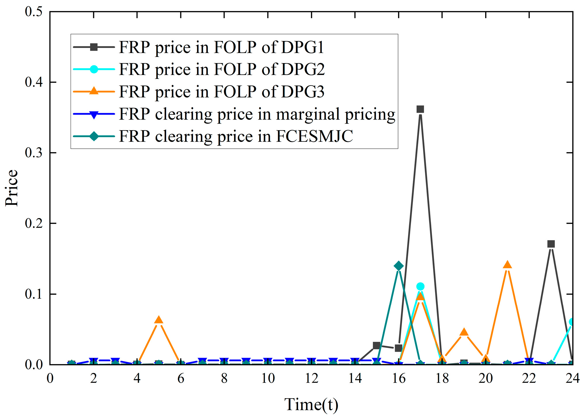
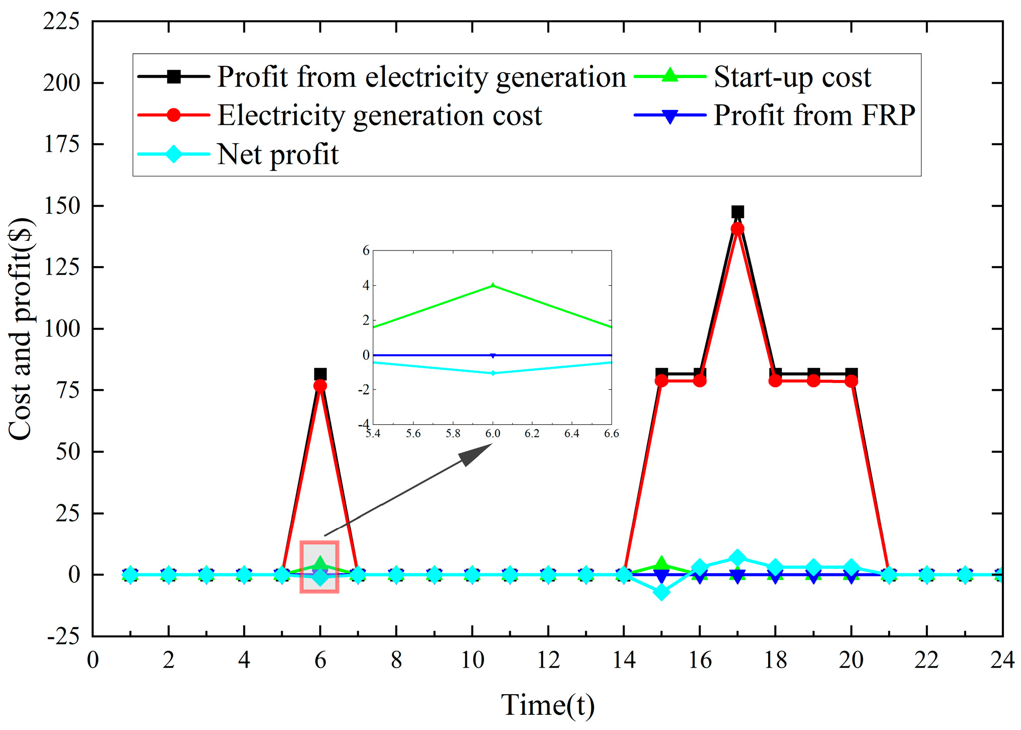
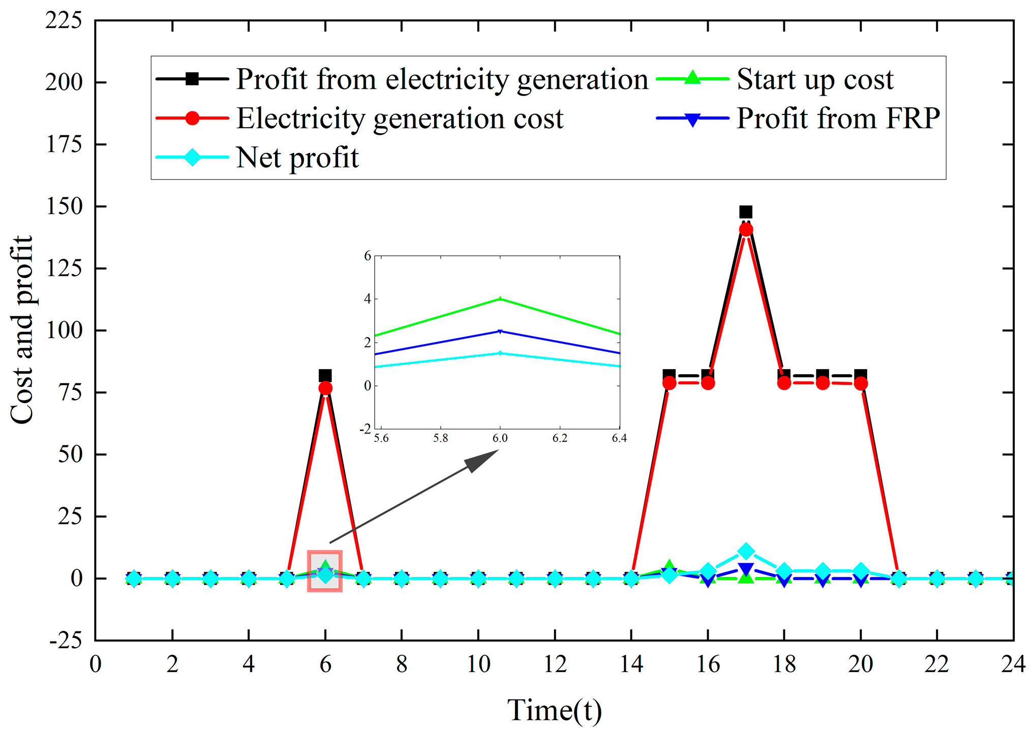
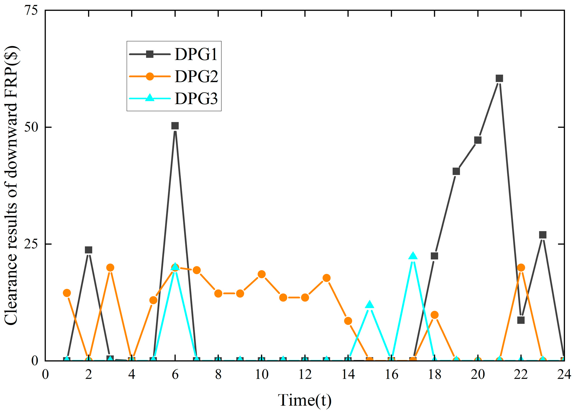
• In the NP-FCE model, the downward FRP price for all DPGs at t = 6 was USD 8 × 10⁻⁶/MW, as shown in Figure 9, and the net profit of DPG3 was USD −1.001, as shown in Figure 10. In the FCESMJC model, using the FOLP method, the downward FRP prices for DPG1, DPG2, and DPG3 at t = 6 were USD 0.114/MW, 0.21514/MW, and 0/MW, respectively, as shown in Figure 9, and the net profit of DPG3 was USD 1.530, as shown in Figure 11. The FRP price for all DPGs in the NP-FCE model at t = 6 was close to 0, and DPG3 operated at a negative net profit. This was not enough to cover the lost opportunity cost of DPG3. In contrast, DPG3 had better economic profit in the FCESMJC model. The proposed FCESMJC model could calculate the FRP price based on the power output of the DPG and LMP and better compensate for the FRP cost of the FRP market participants.
• In the conventional LESM-F model, the generation cost was USD 9092.1337, the FRP cost was USD 0, the accidental cost was USD 2209.1099, and the system cost was USD 11,301.2436, as shown in Table 6. In the proposed FCESMJC-F model, the generation cost was USD 9175.3727, the FRP cost was USD 20.9244, the unexpected cost was USD 0, and the system cost was USD 9196.2971, as shown in Table 6. Compared with the LESM model, although the generation cost and FRP cost of the FCESMJC model increased by 0.68%, the unexpected cost of the system was reduced by improving the ramping capacity of the system, which resulted in a decrease in the system cost by 18.6%. This improved the economic efficiency of the system.

5. Conclusions

The high percentage of fluctuating new energy access poses new challenges to the flexible operation of power systems. FRP is designed to meet the increased demand for DPG ramping capacity by reserving the ramping capacity of an adjustable DPG in advance. In this paper, we proposed a novel FCESMJC market mechanism that reduces spikes in electricity prices, compensates FRP market participants economically, and improves system economics.

Future works may look at joint services between FRP and other products in the electricity market to improve the ramping capacity of the power systems and optimize the market for ancillary services. Additionally, further research on FRP demand is necessary to calculate FRP demand more accurately by considering the stochastic nature of the net load, which is closely related to the operating status of the DGP, the level of active output, and the market clearing price. The conventional calculation of FRP demand is based on renewable energy fluctuations and load forecast errors, and thus a more accurate characterization of renewable energy fluctuations is essential for assessing FRP demand. Procuring FRP products through stochastic and robust optimization is also a future research priority.

References

1. CAISO. 2018 Annual Report on Market Issues & Performance. May 2019. Available online: http://www.caiso.com/Documents/2018AnnualReportonMarketIssuesandPerformance.pdf (accessed on 26 January 2024).
2. Haegel, N.M.; Kurtz, S.R. Global Progress Toward Renewable Electricity: Tracking the Role of Solar. IEEE J. Photovolt. 2021, 11, 1335–1342. [Google Scholar] [CrossRef]
3. Tseng, M.-L.; Eshaghi, N.; Gassoumi, A.; Dehkalani, M.M.; Gorji, N.E. Experimental Measurements of Soiling Impact on Current and Power Output of Photovoltaic Panels. Mod. Phys. Lett. B 2023, 37, 2350182. [Google Scholar] [CrossRef]
4. Wang, Q.; Hodge, B.-M. Enhancing Power System Operational Flexibility With Flexible Ramping Products: A Review. IEEE Trans. Ind. Inform. 2017, 13, 1652–1664. [Google Scholar] [CrossRef]
5. Riaz, S.; Mancarella, P. Modelling and Characterisation of Flexibility From Distributed Energy Resources. IEEE Trans. Power Syst. 2022, 37, 38–50. [Google Scholar] [CrossRef]
6. Mladenov, V.; Chobanov, V.; Georgiev, A. Impact of Renewable Energy Sources on Power System Flexibility Requirements. Energies 2021, 14, 2813. [Google Scholar] [CrossRef]
7. Min, C. Investigating the Effect of Uncertainty Characteristics of Renewable Energy Resources on Power System Flexibility. Appl. Sci. 2021, 11, 5381. [Google Scholar] [CrossRef]
8. Steriotis, K.; Šepetanc, K.; Smpoukis, K.; Efthymiopoulos, N.; Makris, P.; Varvarigos, E.; Pandžić, H. Stacked Revenues Maximization of Distributed Battery Storage Units Via Emerging Flexibility Markets. IEEE Trans. Sustain. Energy 2022, 13, 464–478. [Google Scholar] [CrossRef]
9. Badanjak, D.; Pandžić, H. Battery Storage Participation in Reactive and Proactive Distribution-Level Flexibility Markets. IEEE Access 2021, 9, 122322–122334. [Google Scholar] [CrossRef]
10. California Independent System Operator. Addendum-Draft Final Technical Appendix-Flexible Ramping Product. 2016. Available online: https://www.caiso.com/Documents/Addendum-DraftFinalTechnicalAppendix-FlexibleRampingProduct.pdf (accessed on 26 January 2024).
11. Sreekumar, S.; Sharma, K.C.; Bhakar, R. Multi-Interval Solar Ramp Product to Enhance Power System Flexibility. IEEE Syst. J. 2021, 15, 170–179. [Google Scholar] [CrossRef]
12. Varghese, S.; Dalvi, S.; Narula, A.; Webster, M. The Impacts of Distinct Flexibility Enhancements on the Value and Dynamics of Natural Gas Power Plant Operations. IEEE Trans. Power Syst. 2021, 36, 5803–5813. [Google Scholar] [CrossRef]
13. Khatami, R.; Parvania, M.; Narayan, A. Flexibility Reserve in Power Systems: Definition and Stochastic Multi-Fidelity Optimization. IEEE Trans. Smart Grid 2020, 11, 644–654. [Google Scholar] [CrossRef]
14. Wang, B.; Hobbs, B.F. Real-Time Markets for Flexiramp: A Stochastic Unit Commitment-Based Analysis. IEEE Trans. Power Syst. 2016, 31, 846–860. [Google Scholar] [CrossRef]
15. Pan, H.; Chen, X.; Jin, T.; Bai, Y.; Chen, Z.; Wen, J.; Wu, Q. Real-Time Power Market Clearing Model With Improved Network Constraints Considering PTDF Correction and Fast-Calculated Dynamic Line Rating. IEEE Trans. Ind. Appl. 2023, 59, 2130–2139. [Google Scholar] [CrossRef]
16. Howdhury, M.M.-U.-T.; Biswas, B.D.; Kamalasadan, S. Second-Order Cone Programming (SOCP) Model for Three Phase Optimal Power Flow (OPF) in Active Distribution Networks. IEEE Trans. Smart Grid 2023, 14, 3732–3743. [Google Scholar] [CrossRef]
17. Garifi, K.; Johnson, E.S.; Arguello, B.; Pierre, B.J. Transmission Grid Resiliency Investment Optimization Model with SOCP Recovery Planning. IEEE Trans. Power Syst. 2022, 37, 26–37. [Google Scholar] [CrossRef]
18. Bai, X.; Wei, H.; Fujisawa, K.; Wang, Y. Semidefinite Programming for Optimal Power Flow Problems. Int. J. Electr. Power Energy Syst. 2008, 30, 383–392. [Google Scholar] [CrossRef]
19. Shin, H.; Baldick, R. Optimal Battery Energy Storage Control for Multi-Service Provision Using a Semidefinite Programming-Based Battery Model. IEEE Trans. Sustain. Energy 2023, 14, 2192–2204. [Google Scholar] [CrossRef]
20. Lorca, Á.; Sun, X.A. The Adaptive Robust Multi-Period Alternating Current Optimal Power Flow Problem. IEEE Trans. Power Syst. 2018, 33, 1993–2003. [Google Scholar] [CrossRef]
21. Kim, D.; Kwon, K.; Kim, M.-K. Application of Flexible Ramping Products with Allocation Rates in Microgrid Utilizing Electric Vehicles. Int. J. Electr. Power Energy Syst. 2021, 133, 107340. [Google Scholar] [CrossRef]
22. Chen, S.; Conejo, A.J.; Wei, Z. Power-Gas Coordination: Making Flexible Ramping Products Feasible. IEEE Trans. Power Syst. 2023, 38, 4697–4707. [Google Scholar] [CrossRef]
23. Cha, S.-H.; Kwak, S.-H.; Ko, W. A Robust Optimization Model of Aggregated Resources Considering Serving Ratio for Providing Reserve Power in the Joint Electricity Market. Energies 2023, 16, 7061. [Google Scholar] [CrossRef]
24. Zhong, J.; Chen, H.; Chen, W. Real-time power market clearing with flexibility resource trading. Grid Technol. 2021, 45, 1032–1041. [Google Scholar]
25. Park, H.; Huang, B.; Baldick, R. Enhanced Flexible Ramping Product Formulation for Alleviating Capacity Shortage in Look-Ahead Commitment. J. Mod. Power Syst. Clean Energy 2022, 10, 850–860. [Google Scholar] [CrossRef]
26. Khoshjahan, M.; Dehghanian, P.; Moeini-Aghtaie, M.; Fotuhi-Firuzabad, M. Harnessing Ramp Capability of Spinning Reserve Services for Enhanced Power Grid Flexibility. IEEE Trans. Ind. Appl. 2019, 55, 7103–7112. [Google Scholar] [CrossRef]
27. Zhang, X.; Hu, J.; Wang, H.; Wang, G.; Chan, K.W.; Qiu, J. Electric Vehicle Participated Electricity Market Model Considering Flexible Ramping Product Provisions. IEEE Trans. Ind. Appl. 2020, 56, 5868–5879. [Google Scholar] [CrossRef]
28. Zhang, Z.; Li, F.; Park, S.-W.; Son, S.-Y. Local Energy and Planned Ramping Product Joint Market Based on a Distributed Optimization Method. CSEE J. Power Energy Syst. 2021, 7, 1357–1368. [Google Scholar]
29. PJM Education. Consistency of Energy-Related Opportunity Cost Calculations [EB/OL]. 20 May 2017. Available online: http://citeseerx.ist.psu.edu/viewdoc/download.doi=10.1.1.352.7791&rep=rep1&1&type=pdf (accessed on 26 January 2024).
30. Kocuk, B.; Dey, S.S.; Sun, X.A. Strong SOCP Relaxations for the Optimal Power Flow Problem. Oper. Res. 2016, 64, 1177–1196. [Google Scholar] [CrossRef]
31. Mezghani, I.; Stevens, N.; Papavasiliou, A.; Chatzigiannis, D.I. Hierarchical Coordination of Transmission and Distribution System Operations in European Balancing Markets. IEEE Trans. Power Syst. 2023, 38, 3990–4002. [Google Scholar] [CrossRef]
32. O’Neill, R.P.; Castillo, A.; Eldridge, B.; Hytowitz, R.B. Dual Pricing Algorithm in ISO Markets. IEEE Trans. Power Syst. 2017, 32, 3308–3310. [Google Scholar] [CrossRef]
33. Fiacco, A.V.; McCormick, G.P. Nonlinear Programming: Sequential Unconstrained Minimization Techniques; Society for Industrial and Applied Mathematics: Philadelphia, PA, USA, 1990. [Google Scholar]
34. Wei, H.; Sasaki, H.; Kubokawa, J.; Yokoyama, R. An Interior Point Nonlinear Programming for Optimal Power Flow Problems with a Novel Data Structure. IEEE Trans. Power Syst. 1998, 13, 870–877. [Google Scholar] [CrossRef]
35. California Independent System Operator. Revised Draft Final Proposal-Flexible Ramping Product. 2015. Available online: https://www.caiso.com/Documents/RevisedDraftFinalProposal-FlexibleRampingProduct-2015.pdf (accessed on 26 January 2024).
36. MISO. Ramp Product Questions and Answers [EB/OL]. 31 March 2016. Available online: https://www.misoenergy.org/Library/Repository/Communication%20Material/Strategic%20Initiatives/Ramp%20Product%20Questions%20and%20Answers.pdf (accessed on 26 January 2024).
37. Cornelius, A.; Bandyopadhyay, R.; Patiño-Echeverri, D. Assessing Environmental, Economic, and Reliability Impacts of Flexible Ramp Products in MISO’s Electricity Market. Renew. Sustain. Energy Rev. 2018, 81, 2291–2298. [Google Scholar] [CrossRef]
Figure 1. Schematic calculation of Equations (45) and (46).
Sustainability 16 02390 g001
Figure 2. Schematic calculation of Equations (47) and (48).
Sustainability 16 02390 g002
Figure 3. Flowchart of FCESMJC market mechanism.
Sustainability 16 02390 g003
Figure 4. Single-line diagram of IEEE 14 bus power system.
Sustainability 16 02390 g004
Figure 5. Forecasted net load curve.
Sustainability 16 02390 g005
Figure 6. LESM-F and FCESMJC-F model clearing prices at bus 13.
Sustainability 16 02390 g006
Figure 7. Upward FRP demand and downward FRP demand.
Sustainability 16 02390 g007
Figure 8. Upward FRP price and clearing price from NP-FCE and FCESMJC models.
Sustainability 16 02390 g008
Figure 9. Downward FRP price and clearing price from NP-FCE and FCESMJC models.
Sustainability 16 02390 g009
Figure 10. Cost and benefit curves for DPG3 in NP-FCE model.
Sustainability 16 02390 g010
Figure 11. Cost and profit curves for DPG3 in FCESMJC-N model.
Sustainability 16 02390 g011
Figure 12. Clearing results of upward FRP.
Sustainability 16 02390 g012
Figure 13. Clearing results of downward FRP.
Sustainability 16 02390 g013
Figure 14. LESM system load and DPG active output.
Sustainability 16 02390 g014
Figure 15. FCESMJC system load and DPG active output.
Sustainability 16 02390 g015
Figure 16. Bus phase angle from FCESMJC model at  t  = 1.
Sustainability 16 02390 g016