Abstract
Comprehensively and objectively revealing the spatial relationship between ecosystem services (ESs) and human activity intensity (HAI) is vital for achieving sustainable development goals. However, existing studies still have an incomplete understanding of how ESs change with HAI gradients. Therefore, taking Shenzhen City, China, as an example region experiencing rapid urbanization, the distribution of ESs and HAI in 2010 and 2020 were quantified using the InVEST model and the human footprint index method; at the same time, the gradient perspective was introduced and the spatial and temporal correlation characteristics of ESs along 10 HAI gradient bands, from weak to strong, were captured by applying multiscale geographically weighted regression (MGWR) and the bivariate spatial autocorrelation model. The findings showed that (1) the HAI demonstrated an increasing trend (20.63 (2010) and 23.36 (2020)), and the area with high values of HAI (the 10th gradient band) was distributed in the western part of the study area; meanwhile, the area with low HAI values (the 1st gradient band) was more distributed in the eastern part of the study area. (2) On the whole, the average levels of water conservation, soil conservation, carbon storage, and habitat quality decreased from 2010 to 2020; the spatial distribution characteristics of these parameters were similar. (3) In general, ESs were negatively correlated with HAI, and the negative correlation ratio was more than 65%. At the same time, the spatial and temporal correlations between ES patterns and HAI under different gradient bands were significant. These findings can effectively alleviate the pressure on the ecosystem caused by human activities, which is of great significance for the sustainable development of highly urbanized regions.
1. Introduction
Human activity intensity (HAI) refers to the degree of disturbance caused by human activities in a certain area [1]; as a universal phenomenon in nature, HAI directly or indirectly affects the succession of ecosystems [2]. Ecosystem services (ESs) are defined as benefits or contributions provided by natural ecosystems that can be utilized by humans [3,4]; these services are the material basis for human survival and development, and are the bridge between natural ecosystems and human beings [5]. In recent years, the United Nations 2030 Agenda and the Sustainable Development Goals (SDGs) have aimed to reduce the impact of human activities on the ecological environment and improve human well-being [6]. It can be seen that understanding the relationship between HAI and ESs is an urgent problem that must be solved, in order to achieve the sustainable development of human society [7]. Currently, rapid population growth and urbanization have led to the substantial shrinkage of ecological land and serious environmental pollution, both of which have brought severe environmental pressure to the global ecological environment [8]. The impact of this will continue to expand and intensify in the future, with its obvious gradient characteristics, long-term evolution, and adaptation process [9]. Therefore, exploring and quantifying the spatial characteristics of ESs along gradients of HAI can provide theoretical guidance for the rational control of human activities and maintenance of service functions.
With the development of spatial analysis technology, the traditional non-spatialization methods (i.e., statistical analysis methods) are gradually facing more difficulty in meeting the needs of various types of applications; research on the spatialization of HAI has begun to develop, and various methods of direct or indirect spatialization have been put forward and widely used [10]. First, indirect spatialization methods include the vegetation index method [11], the human appropriation of net primary production (HANPP), and the global disturbance index method. Among these, the HANPP method has better evaluation results, can also reflect the positive impacts of human activities, and has been applied at different scales [12]. However, the method needs to be coupled with statistical data, resulting in the insufficient spatial refinement of the data [13]. The global disturbance index method couples surface temperature with the enhanced vegetation index, in order to characterize the intensity [14]. Nonetheless, this method makes it difficult to isolate the human factors, making it more suitable for large-scale vegetation belts. Second, direct spatialization methods include the land use type change method, the comprehensive indicator method [15], and the human footprint index method. Among these, the land use change method evaluates HAI using a model based on construction land, and then spatially expresses the evaluation results [10]. It has been applied at different spatial scales. The comprehensive indicator method [16] considers that HAI is the result of the combined effects of natural environmental conditions and human socio-economic activities. However, the data prepared by this type of method mainly take the county as the smallest spatial unit, with poor spatial refinement, and this applies to regions where administrative units are the object of study [17]. The human footprint index method was proposed by Sanderson and other scholars [18], and this method selects spatial data, such as population density, land use change, and roads, to quantify HAI [19], which can make up for the weaknesses of previous findings that were only calculated using a single indicator of landscape change or land use change. In general, the study of the human footprint index method has made some progress; this method is more suitable for quantifying HAI in land systems at a grid scale [20]. However, in quantifying HAI, the methodology has a wide accuracy range in terms of data selection, which means it has difficulties generalizing all human activities and may underestimate HAI to a certain extent; thus, it still needs to be improved and optimized [21,22]. Therefore, based on the research results of the human footprint index method, this study fully considers the economic and social development of the high-speed development area, and adds the urban facility density layer (POI data) to represent the spatial distribution of HAI.
Various researchers have conducted more elaborate studies on the classification of ESs, such as Costanza et al. [23], Ouyang et al. [24], Xie et al. [25], and Millennium Ecosystem Assessment [26], all of whom elaborated on the classification system. Among them, MA is an influential classification system, which mainly includes provisioning services, regulating services, supporting services, and cultural services; it is widely acknowledged and employed by scholars in the academic field [27]. Existing studies have found that ES evaluation has mainly focused on the evaluation of service provision and regulation, with many studies on land use change and ESs, but few studies on support and cultural services [28]. In the meantime, ES evaluation methods have undergone a long development process from simple ES measurement (quality and value) to the current composite model method [29]. In recent years, research on ESs has become widespread in countries around the globe, focusing mainly on service frameworks, developing value assessment methodologies, and analyzing internal trade-offs [30]. From the perspective of research objects and spatial scope, the research objects regarding ESs have become broader, their spatial scope has expanded, and their application fields have become more diversified. The research objects involve ecologically fragile areas [31], river basins [32], hills and mountains [33], etc. With the rapid development of remote sensing technology, InVEST, ARIES, MIMES, and other models have been applied for evaluating ESs [34], but the emphases of these models are different. Among them, the InVEST model is the most systematic; not only does it have a strong spatial analysis function, but its low application cost, strong open source, high assessment accuracy, etc., are also superior to other models [35]. Therefore, it is widely used in current ecosystem assessment models.
Changes in HAI affect the changes in the ecosystem structure, function, and service, posing a threat to the ecosystem’s balance and the sustainable development of society and the economy [2,36]. However, due to the complexity and uncertainty of human activities [37], the interaction mechanism between HAI and ESs is still being explored. Currently, many studies have discussed the changing trend in the relationship between HAI and ESs from different perspectives [20,38] and have reached different conclusions. For example, Qi et al. [39] used the Sanderson human footprint model and InVEST model to measure human activities and ecosystem services in the Qinghai Lake Basin, China, and simulated the influence curves of human activities on six types of ecosystem services, including carbon storage, habitat quality, soil erosion, and water yield, through the generalized additive model. This model also reveals the evolution of complex nonlinear relationships between human activities and these types of ESs. Existing studies show that most studies start from the perspective of exploring the correlation between them, and often fail to fully and specifically reveal their roles under different gradients. In terms of research methodology, scholars have further explored the quantitative correlation between human activities and environmental systems with the help of coupled coordination models [20], while less research has been conducted on the spatial correlation between HAI and ESs, as well as on the spatial distribution of the degree of correlation. There needs to be more research on whether a spatial autocorrelation exists between HAI and ESs [1], what kinds of characteristics that spatial aggregation may present, and whether the spatial relationship between the two evolves with spatial and temporal changes. In real contexts, there are different scales of action for the effect of HAI on ESs, and thus a single bandwidth cannot well reflect the spatial process of the action intensity between variables [40]. Based on this, Fotheringham et al. [41] proposed the use of multiscale geographically weighted regression (MGWR) for estimating the spatial bandwidths of variable differentiation based on traditional geographically weighted regression (GWR), which better solves the defects of a single bandwidth of the GWR model, and has become an important method for revealing the impacts and the scale of the effects between variables. Therefore, this study adopts the bivariate spatial autocorrelation method and the MGWR model to explore the relationship and clustering patterns between human activities and ESs under different gradients.
Thanks to the depth of research on this topic, the theoretical and methodological system for quantifying ESs and HAI has gradually improved. However, there are some shortcomings: (1) more attention has been paid to the study of ecologically fragile areas, but fewer studies have focused on areas with higher levels of economic development; and (2) most of the existing studies are limited to the quantitative relationship between HAI and ESs, which, to some extent, limits the disclosure of their complex interactions from a gradient perspective. In coastal cities with rapid economic development, such as Shenzhen, China, human development activities are more frequent and intense due to the need to source land from the sea in order to meet the social development requirements. ESs face a significant challenge, which greatly hinders the sustainable development of the economy in the Greater Bay Area [42]. In summary, we studied the distribution of HAI and ESs in Shenzhen by analyzing spatial and temporal geographic data with the InVEST model, human footprint index method, MGWR model, and the bivariate spatial autocorrelation model. We also aimed to divide HAI into multiple gradient bands from weak to strong, and explore the relationship between different gradients of HAI and ESs. The research objectives are as follows: (1) to understand the spatial and temporal characteristics of ESs and HAI in economically developed areas and (2) to explore the relationship between gradient differences in ESs and gradient changes in HAI. This study overcomes the deficiencies of existing research findings and explores the spatial relationship between HAI and ESs from a gradient perspective, in order to provide data support and a scientific basis for the sustainable development in high-utilization urban areas.
2. Materials and Methods
2.1. Study Area
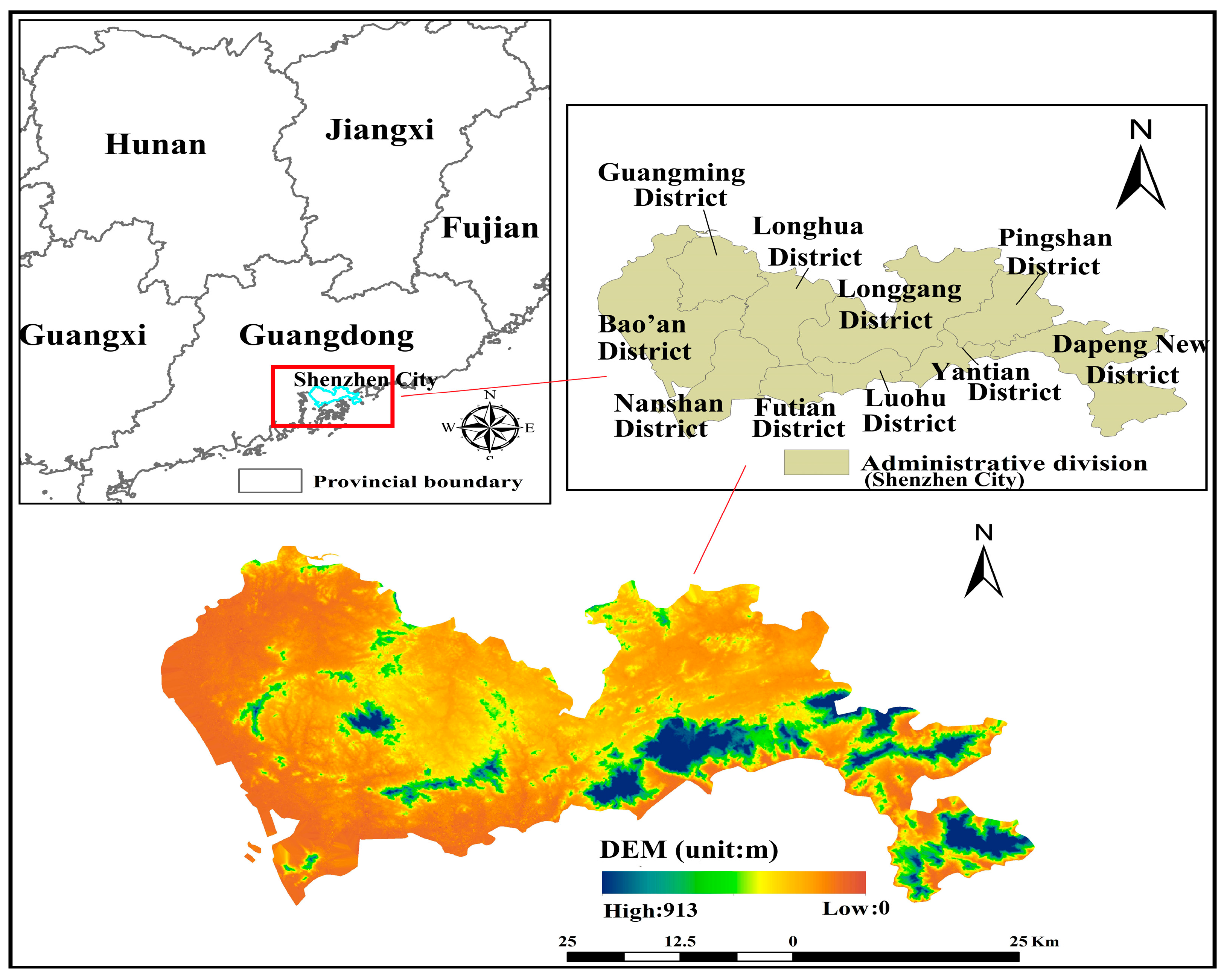
Shenzhen City (113°45′~114°37′ E, 22°26′~22°51′ N) is located to the south of the Tropic of Cancer, in the southern coastal area of China, with low terrain in the northwest and high in the southeast (the average elevation is about 80 m), and is one of the four central cities in the Guangdong–Hong Kong–Macao Greater Bay Area (Figure 1). The land area of the study area is approximately 1997.47 km2, of which approximately 1005.95 km2 is built up, accounting for approximately 50.36% of the city; meanwhile, the topography of the area is low in the northwest and high in the southeast. In the continuous development and construction of urbanization in the study area, urban green space has been increasingly eroded, fragmentation is serious, and eco-environmental problems are becoming increasingly prominent, which seriously affects regional ESs [43].
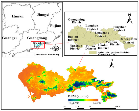
Figure 1.
Location of study area.
2.2. Data Sources
The four sub-modules of the InVEST model selected in this study were water conservation (water yield), carbon storage, soil conservation, and habitat quality. The data requirements of each module of the InVEST model are shown in Table 1. Secondly, the human footprint index method mainly involves population, night-time lighting, land use, and point of interest (POI) data, the sources of which are detailed in Table 1.

Table 1.
Summary of main data types and data sources.
2.3. Methods
2.3.1. ESs Based on InVEST Model
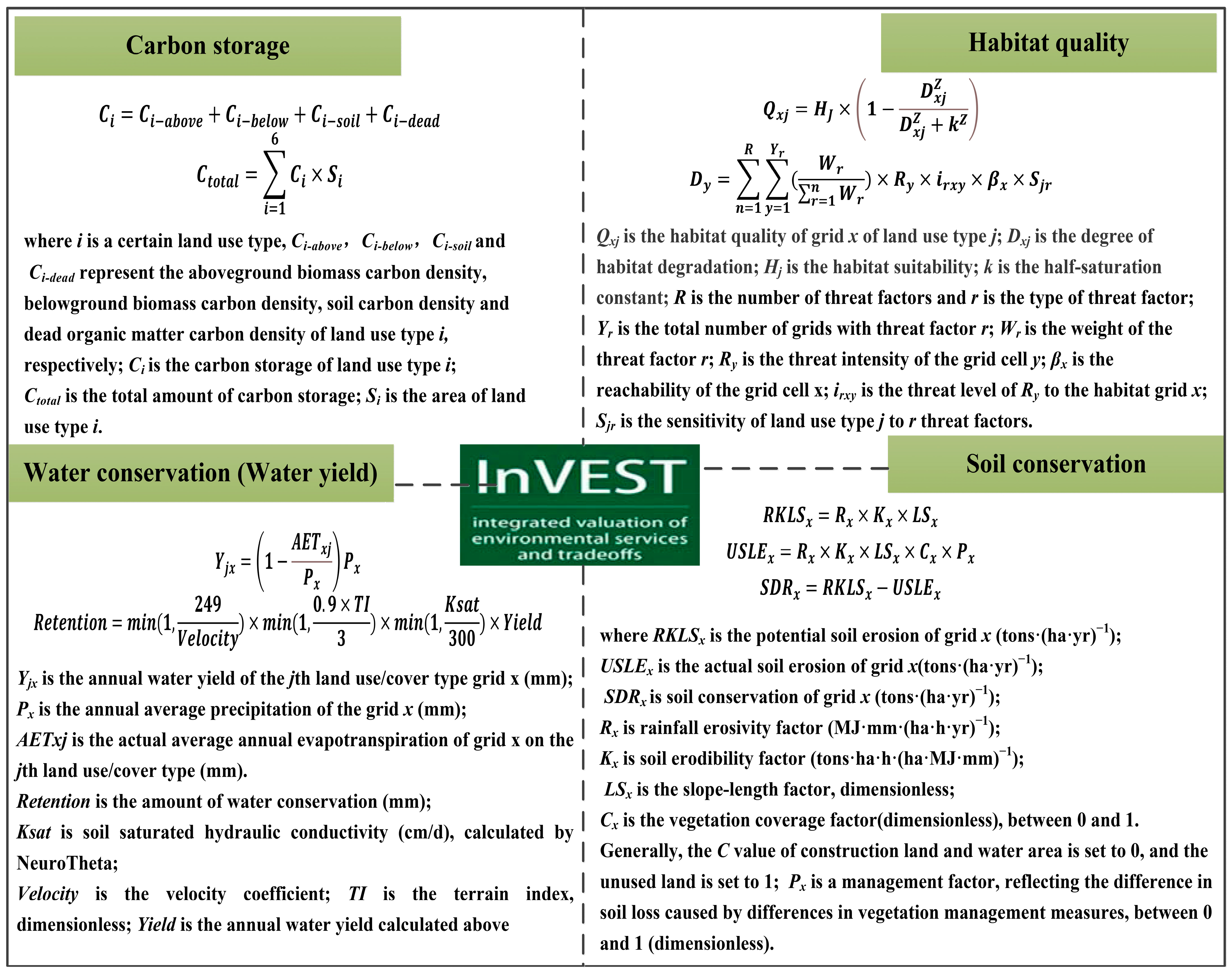
This study used multiple modules of the InVEST model (Figure 2), a model system used to assess ESs in order to support ecosystem management and decision making. The module was set by referring to the InVEST Model User Guide [44] and to previous research results [45,46]. The specific setting parameters are shown in Table 2 and Table 3.
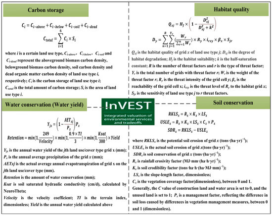
Figure 2.
Principles of ES estimation based on InVEST.
Table 2.
Threat factors in the Habitat Quality module.
Table 3.
Relevant parameters in carbon storage, soil conservation, and water conservation.
2.3.2. Quantitative Modeling of HAI
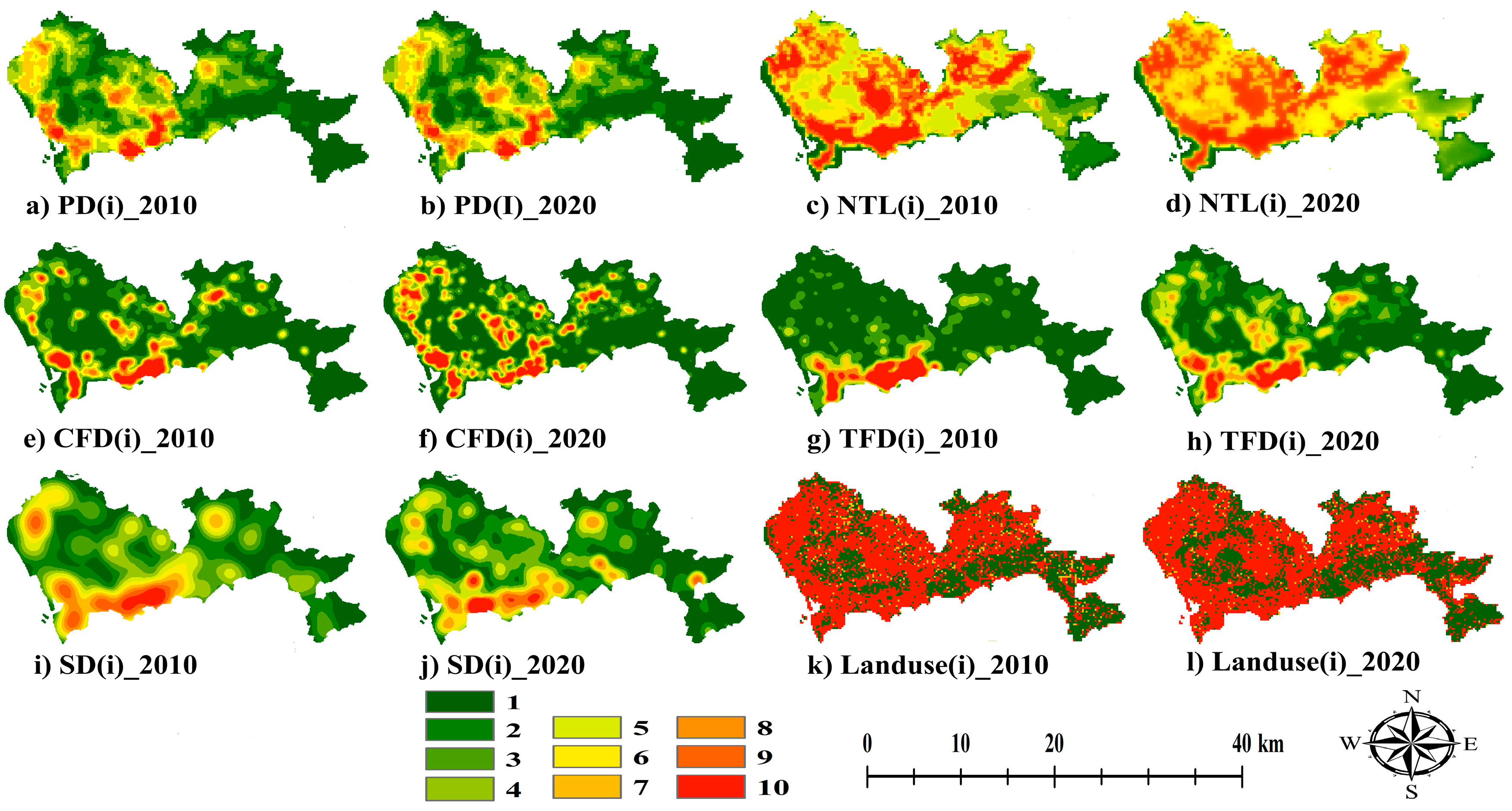
Based on the human footprint index method, six types of human activity characterization factors—namely land use, population density, night-time lighting index, scenic area (POI data), commercial facility (POI data), and transport facilities (POI data)—were finally selected based on the actual development of the study area and previous studies [20], and combined with data availability. The formula is as follows:
where Value(i) represents the HAI, landuse(i) is the land use index after assignment quantification, PD(i) is the population density after assignment quantification, TFD(i) is the transport facility density index after assignment quantification, SD(i) is the scenic spot density index after assignment quantification, NTL(i) is the night-time lighting index after assignment quantification, and CFD(i) is the commercial facility density index after assignment quantification (Figure 3).
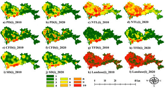
Figure 3.
Spatial distributions of each index based on the human footprint index method.
The specific assignment method is as follows:
- (1)
- Population density
In this study, grid pixels with population densities greater than 1000 person/km2 were assigned a value of 10, while those with population densities equal to 0 person/km2 were assigned a value of 1; the rest of the grid pixels, with population densities between 0 and 1000 person/km2, were assigned a value from 2 to 9 (from smallest to largest) using the equal division method.
- (2)
- Land use
The land use data constitute an important factor reflecting human activities; this study assigned a value of 10 to all construction land, 7 to cropland, and the rest of the land use types were assigned a score of 1.
- (3)
- Night-time lighting
The DN values of night-time lighting data were corrected to be between 0 and 63; secondly, a grid with a DN value equal to 0 was assigned as 1; finally, the rest of the raster data, with DN values greater than 0, were assigned 2–10 (from smallest to largest) using the equal division method.
- (4)
- Scenic area, commercial facility, and transport facilities (POI data)
The kernel density analysis function of GIS was used to obtain the density values of scenic area, commercial facilities, and transport facilities according to a 1 km search radius; secondly, using the normalization method, the density value was normalized as 0–1; finally, the assignment steps were the same as for night-time lighting data.
2.3.3. Driving Mechanism Analysis
First, in this study, the MGWR model (the open-source platform MGWR 2.2 was used) was used to measure the spatial heterogeneity in the pattern and intensity of the interactions between ESs and HAI at different gradients. Compared to the traditional GWR model, MGWR improves the GWR model by allowing the bandwidths of the individual variables to differ, which, in turn, generates more plausible estimates [40,47]. The MGWR model is formulated as follows:
where denotes HAI (response variable), denotes each ES (covariate), is the total number of spatial units involved in the analysis, denotes the random error term, and is the jth local regression coefficient with bandwidth bw. In addition, the MGWR model was built based on GWR estimation as the initial setting, and the quadratic kernel function and Akaike Information Criterion (AICc) methods were used in this study to determine the optimal bandwidth.
Second, the bivariate spatial autocorrelation can reveal the spatial distribution correlation and dependence characteristics between variables [48]. The bivariate Moran index is used to detect the correlation in the spatial distribution of variables and is between −1 and 1; when it is closer to 0, this indicates a smaller spatial correlation between two variables. The resulting aggregate graph can represent the local high value of ES–high value of HAI (H-H)/low value of ES–low value of HAI (L-L) spatial positive correlation between variables, or the high value of ES–low value of HAI (H-L)/low value of ES–high value of HAI (L-H) spatial negative correlation between variables.
where N represents the total number of spatial units; and represent the values of variables m and n in the i and j region units, respectively; and represent the average value of the two variables m and n, respectively; and represent the standard deviation of m and n variables, respectively; and represents the weight of the space between two regions, i and j.
3. Results
3.1. Changing Characteristics of ESs
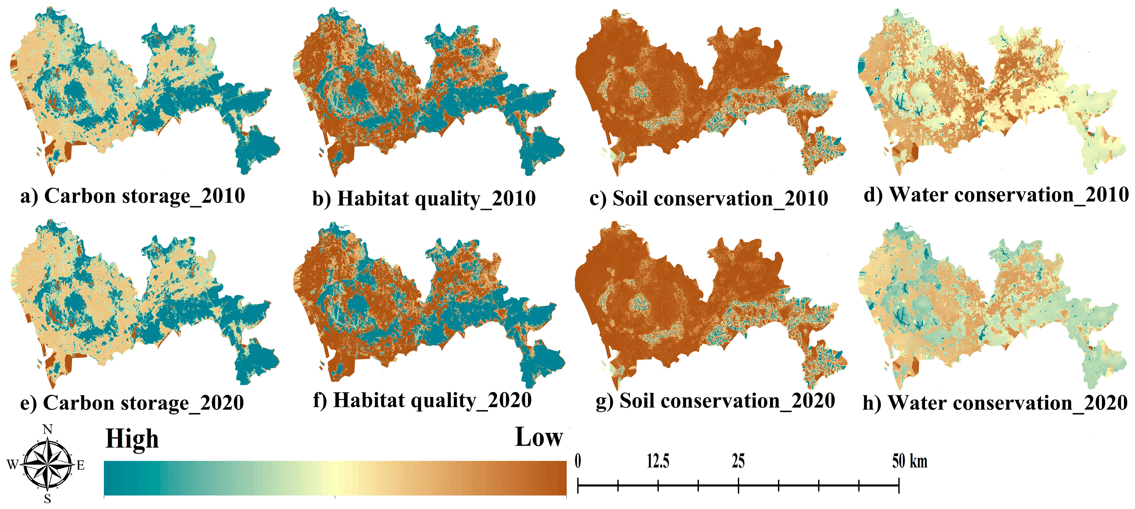
This study used the InVEST (Version 3.10.2) model to quantify and spatially map ESs in the study area. From 2010 to 2020, the average levels of water conservation, soil conservation, carbon storage, and habitat quality showed general downward trends. Furthermore, from 2010 to 2020, the spatial patterns of ESs were similar.
First, the mean value of carbon storage decreased by 0.051 t/km2 (3.158 t/km2 in 2010 and 3.107 t/km2 in 2020). At the same time, the carbon storage spatial pattern was high in the east and low in the west. Among these, the low-value zones were mainly concentrated in construction land and waters; the high-value zones were mainly dominated by forested land, with high carbon densities and high carbon sequestration capacities (Table 4 and Figure 4a,e).
Table 4.
Average level of ESs per unit area.

Figure 4.
Spatial analysis of ESs from 2010 to 2020.
Second, the mean value of habitat quality decreased by 0.017 (0.464 in 2010 and 0.447 in 2020). At the same time, the high-value zones were distributed in high-altitude areas (southeast and west in the study area), with excellent natural conditions suitable for biological survival and a high level of biodiversity, while the low-value zones were mainly distributed in urban areas, whose habitats had been severely damaged by urbanization and development (Table 4 and Figure 4b,f).
Third, the mean value of soil conservation decreased by 0.191 103 t/km2 (1.720 103 t/km2 in 2010 and 1.529 103 t/km2 in 2020). At the same time, the high-value zones were mainly concentrated in the southeast and western parts of the study area. Although the soil was easily eroded due to the large slope, the surface vegetation was dense and the forest land dominated, thus creating a better preservation effect on the soil. While the low-value zones were flat and human activities were frequent, the degree of development was high, mostly for construction land, cultivated land, and water area; the soil was easily eroded (Table 4 and Figure 4c,g).
Fourth, the mean value of water conservation decreased by 0.232 103 m3/km2 (1.498 103 m3/km2 in 2010 and 1.266 103 m3/km2 in 2020). At the same time, the low-value area was mainly construction land and water areas, with low vegetation coverage rates, significant evapotranspiration, and less rainfall than the central area, resulting in a lessened annual water quantity. In the high-value region, the annual precipitation was more abundant, the woodland was widely distributed, and the precipitation was strongly intercepted; thus, the water conservation function was stronger (Table 4 and Figure 4d,h).
3.2. Changing Characteristics of HAI
In terms of time scale, during the period from 2010 to 2020, the mean HAI values in the study area showed an increasing trend (20.63 (2010) and 23.36 (2020)). Moreover, HAI showed an expanding trend during the study period. Specifically, the Luohu District, Futian District, and Nanshan District had higher mean HAI values (above 25). Secondly, the Longgang District, Longhua District, Guangming District, and Bao’an District had medium HAI levels, with mean values mainly between 20 and 25. Finally, the Dapeng New District, Yantian District, and Pingshan District had lower HAI, with mean values below 20 (Table 5).
Table 5.
The mean HAI values of each district and county in the study area.
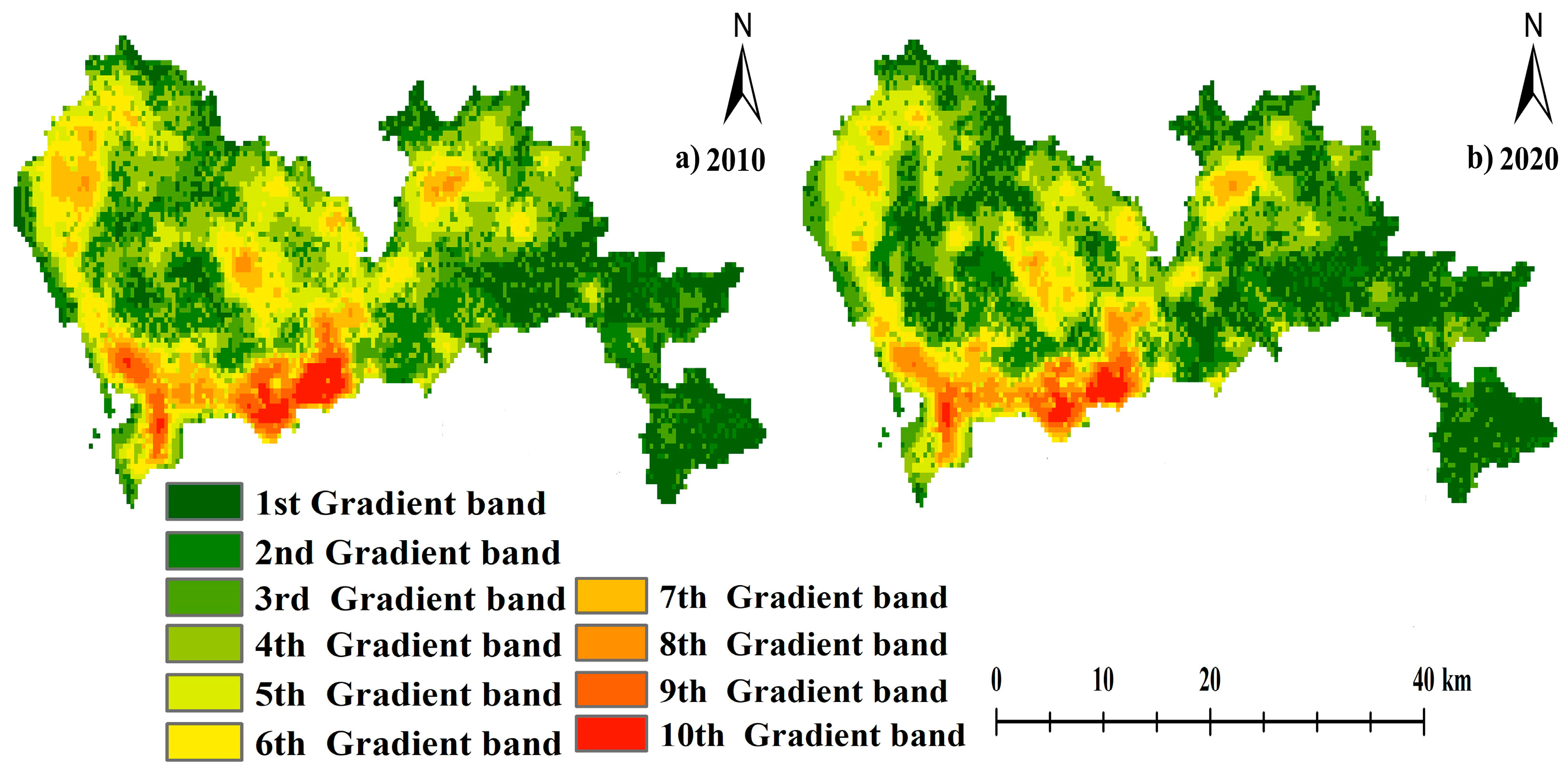
In this study, based on the HAI assessment results, we classified 10 gradients with the help of the average breakpoint method, in which the first gradient band was 0 < HAI ≤ 6, the second gradient band was 6 < HAI ≤ 12, the third gradient band was 12 < HAI ≤ 18, the fourth gradient band was 18 < HAI ≤ 24, the fifth gradient band was 24 < HAI ≤ 30, the sixth gradient band was 30 < HAI ≤ 36, the seventh gradient band was 36 < HAI ≤ 42, the eighth gradient band was 42 < HAI ≤ 48, the ninth gradient band was 48 < HAI ≤ 54, and the tenth gradient band was 54 < HAI ≤ 60. In terms of the spatial scale, there was significant spatial variability in the HAI (first gradient band to tenth gradient band), with HAI in the western part of the study area being higher than that in the eastern part. Among the gradients, the eighth to the tenth bands were mainly concentrated in the southwestern part of the study area, and were located in the region where construction land was concentrated. The first to the third gradient bands were mainly concentrated in the southeastern part of the study area and located in regions with high vegetation cover; the fourth to the seventh gradient bands were mainly concentrated in the northwestern, northeastern, and central parts of the study area. At the same time, the high-intensity regions in the study area were surrounded by medium-intensity areas, while the medium-intensity areas were surrounded by low-intensity areas (Figure 5).

Figure 5.
Spatial distributions of HAI.
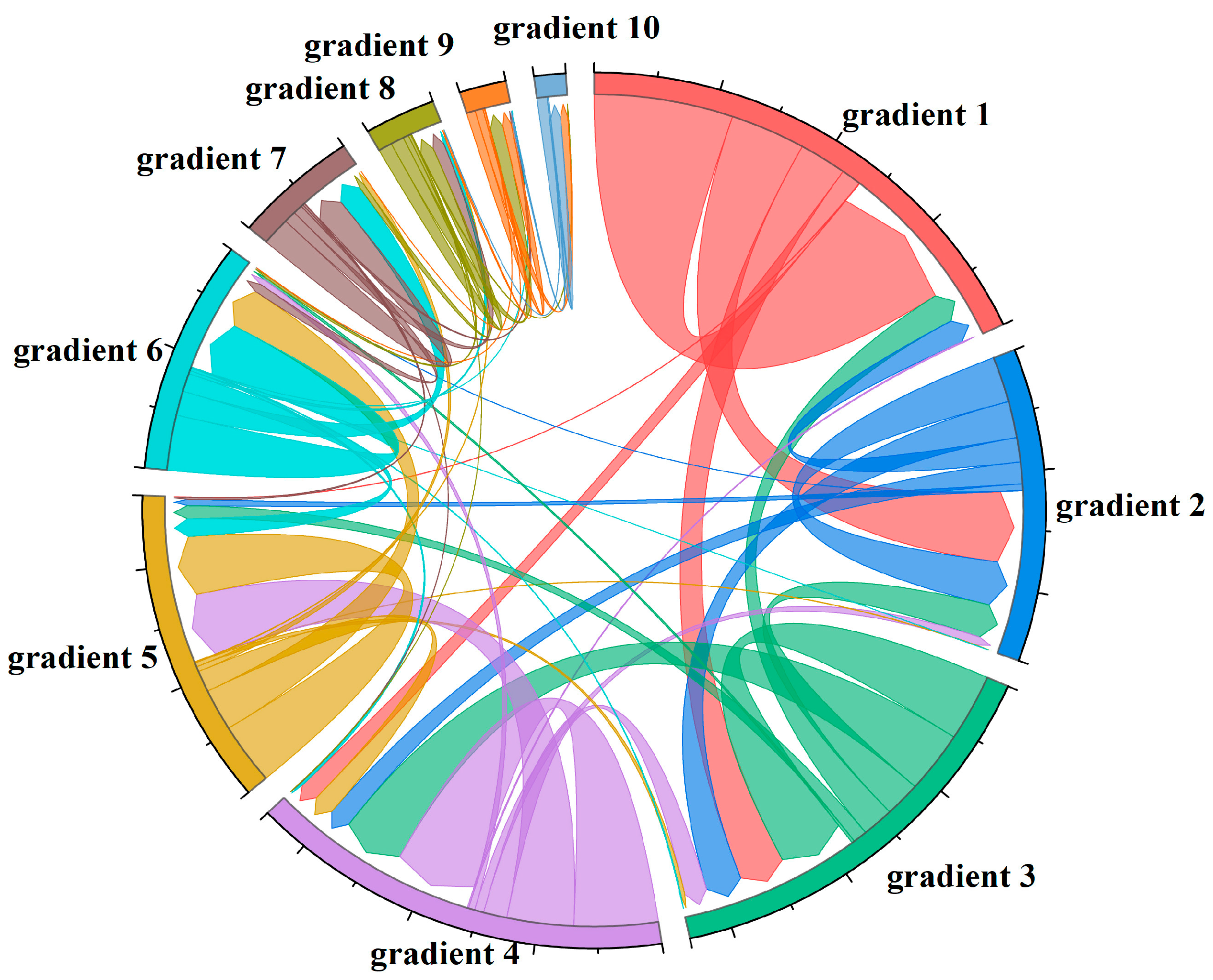
A comparison of HAI in 2010 and 2020 revealed that most of the gradient bands shifted from low to high, and the area transferred out was larger than the area transferred in. Firstly, the first gradient band accounted for the highest total area in 2010 and 2020, and this gradient band mainly shifted to the second–fourth gradient bands. The highest region was transferred to the second gradient band, which accounted for 6.30% of the total area, and the lowest region was transferred to the fourth gradient band, which accounted for 1.67% of the total area. Secondly, the region transferred out of the second–fourth gradient bands was around 5% of the total area. In particular, the transfer from the third to the fourth gradient band accounted for 5.30% of the total area, while the transfer from the fourth to the fifth gradient band accounted for 5.59% of the total area. Finally, the region transferred out of the 5th–9th gradient bands was about 3% of the total area. In particular, the transfer from the fifth gradient band to the sixth gradient band was 3.60% of the total area, and the transfer from the ninth gradient band to the tenth gradient band was 0.64% of the total area (Figure 6).

Figure 6.
Gradient transfers of HAI in study area from 2010 to 2020.
3.3. Gradient Response of ESs Pattern Based on HAI
3.3.1. Changes in ESs along Gradients of HAI
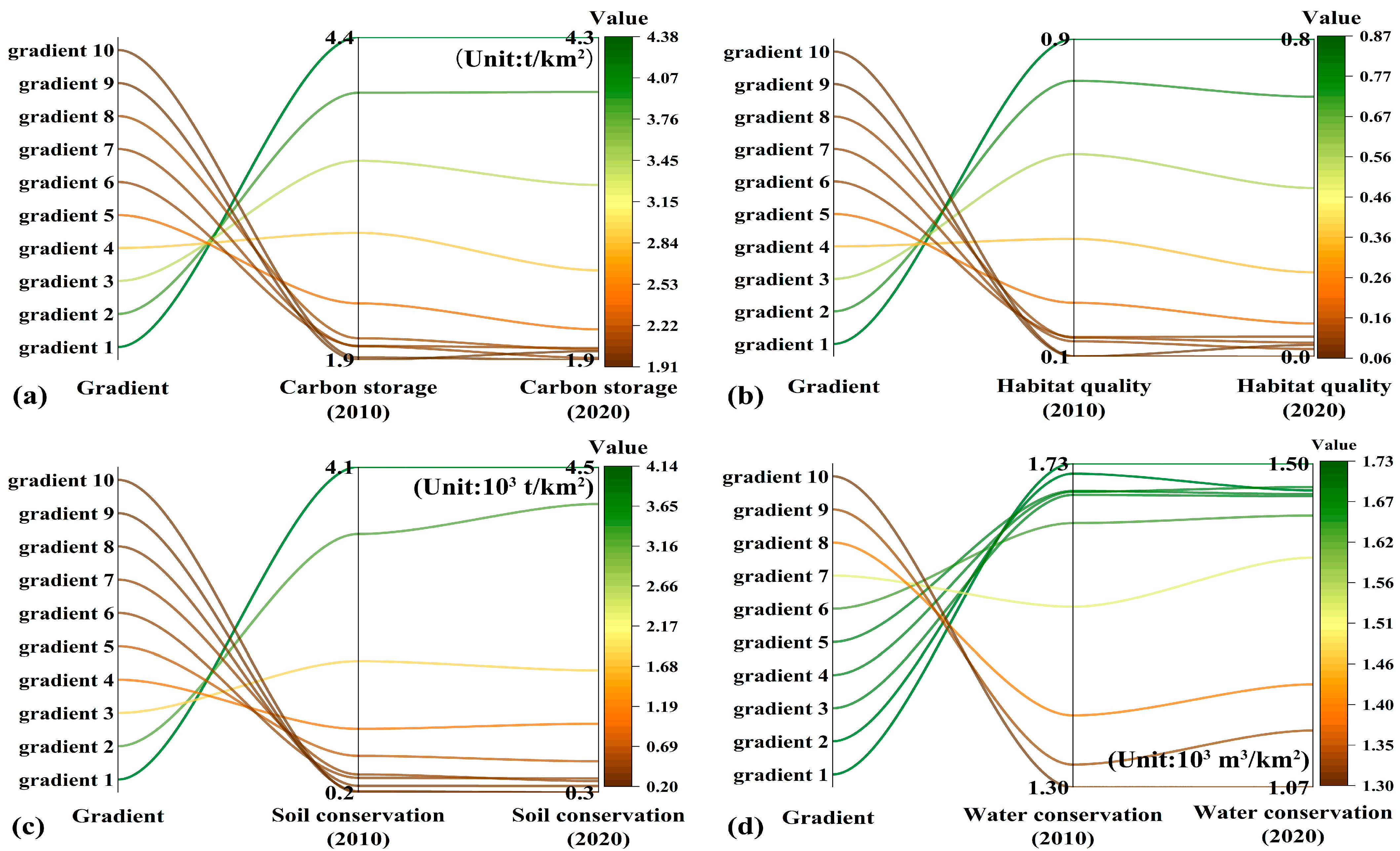
The ESs under gradient bands with different HAIs were summarized and mapped. When the HAI increased (1st–10th gradient bands), carbon storage, habitat quality, soil conservation, and water conservation showed decreasing trends in both 2010 and 2020. Among these, the average values of each ES reached high values in the first gradient band, whereas the average values of each ES in the ninth or tenth gradient band reached low values (Table 6). In addition, the variations in carbon storage, habitat quality, and soil conservation were relatively similar. There was a stepwise decrease in the levels of the three services in the 1st–6th gradient bands, and a more gradual change in the levels of the three services in the 7th–10th gradient bands; the change trends in water conservation were somewhat different. In the 1st–6th gradient bands, the range of service changes was small, while, in the 7th–10th gradient bands, there was a stepwise decrease in the service (Figure 7a–d).
Table 6.
The mean values of ESs based on gradient bands.
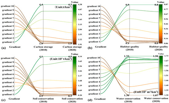
Figure 7.
The variations in ESs under different gradients of HAI.
3.3.2. Agglomeration Type between ESs and HAI at Different Gradients
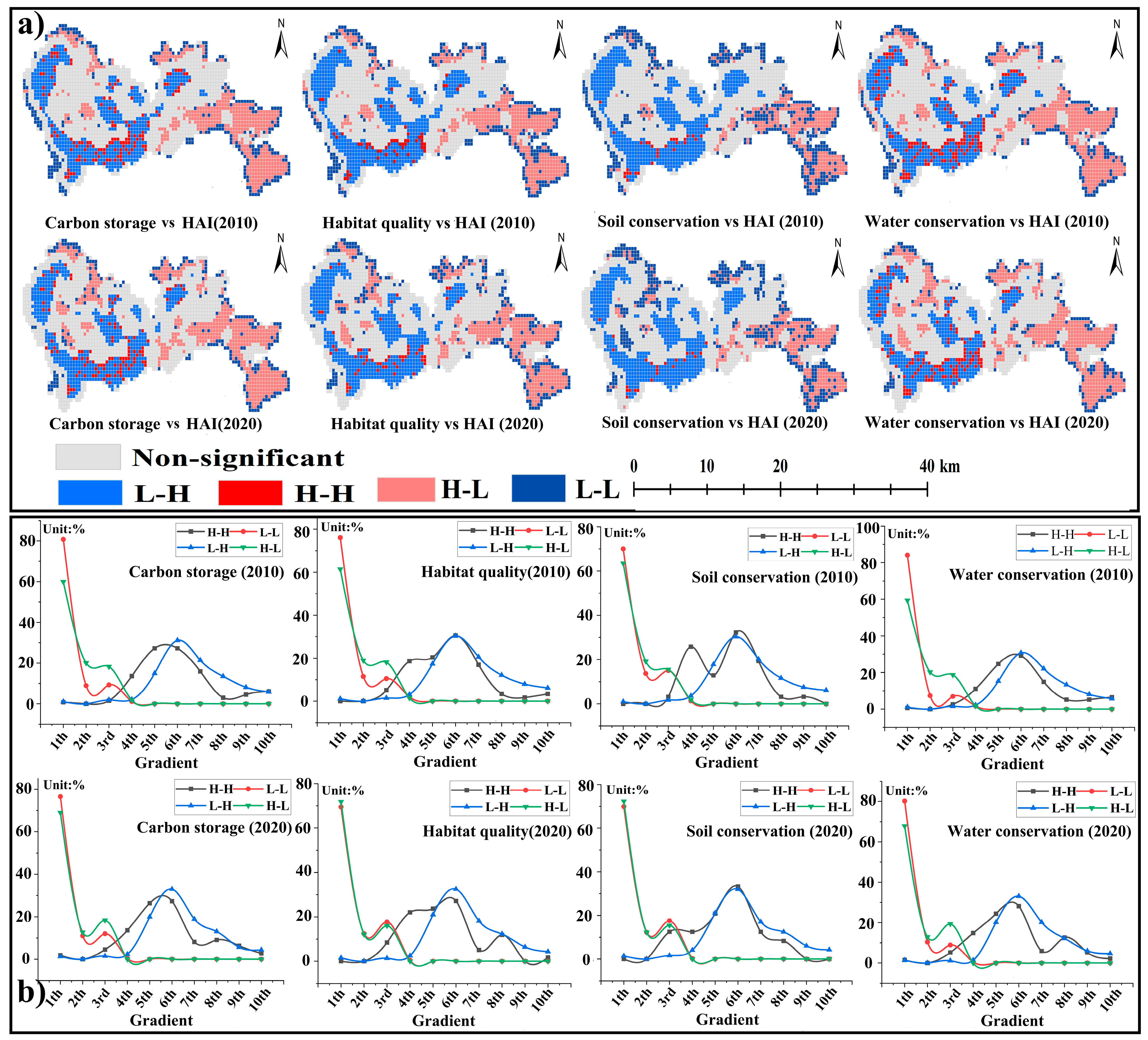
The relationships between ESs and HAI were negative. Among these, the Moran’s I between carbon storage and HAI was −0.183 (2010) and −0.223 (2020); the Moran’s I between habitat quality and HAI was −0.358 (2010) and −0.362 (2020); the Moran’s I between soil conservation and HAI was −0.216 (2010) and −0.206 (2020); and the Moran’s I between water conservation and HAI was −0.073 (2010) and −0.095 (2020) (Table 7). At the same time, in order to deeply grasp the relationship and spatial aggregation characteristics between ESs and HAI, this study was based on a bivariate spatial autocorrelation model. Firstly, in the 1st–4th gradient bands, the L-L and H-L agglomeration types dominated, showing a decreasing trend, while the 5th–10th gradient bands contained almost none of the above agglomeration types. Secondly, in the 3th–10th gradient bands, the H-H and L-H aggregation types dominated, showing an increasing and then decreasing trend, and reaching a peak in the sixth gradient band (Figure 8a,b). In addition, the spatial agglomeration types of ESs and HAI showed variability in different gradient bands, mainly reflecting the first gradient band and sixth gradient band. In the first gradient band, the main spatial agglomeration types were L-L and H-L, which accounted for between 60% and 80% of the corresponding aggregation types. In the sixth gradient band, the main spatial agglomeration types were H-H and L-H, which accounted for about 30% of the corresponding aggregation types (Figure 8b).
Table 7.
ESs and HAI in Moran’s I.
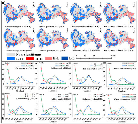
Figure 8.
Spatial aggregation characteristics of ESs and HAI. (a) Spatial agglomeration types of ESs and HAI; (b) spatial agglomeration types of ESs and HAI on different gradient bands.
3.3.3. Interactive Relationship between ESs and HAI at Different Gradients
Compared with the classical GWR model, the AICc value of the MGWR model was smaller, and the adj.R2 reached 0.816 (2010) and 0.821 (2020); these values were both higher than those of the GWR model (0.695 (2010) and 0.638 (2020)), indicating that the fitting results of the MGWR model were superior. Secondly, the bandwidth of classical GWR was 3185.75, while, based on the MGWR model, the variable bandwidths were richly valued, which could directly reflect the average of the differentiated action scales of different variables (Table 8).
Table 8.
Parameters related to MGWR and GWR running results.
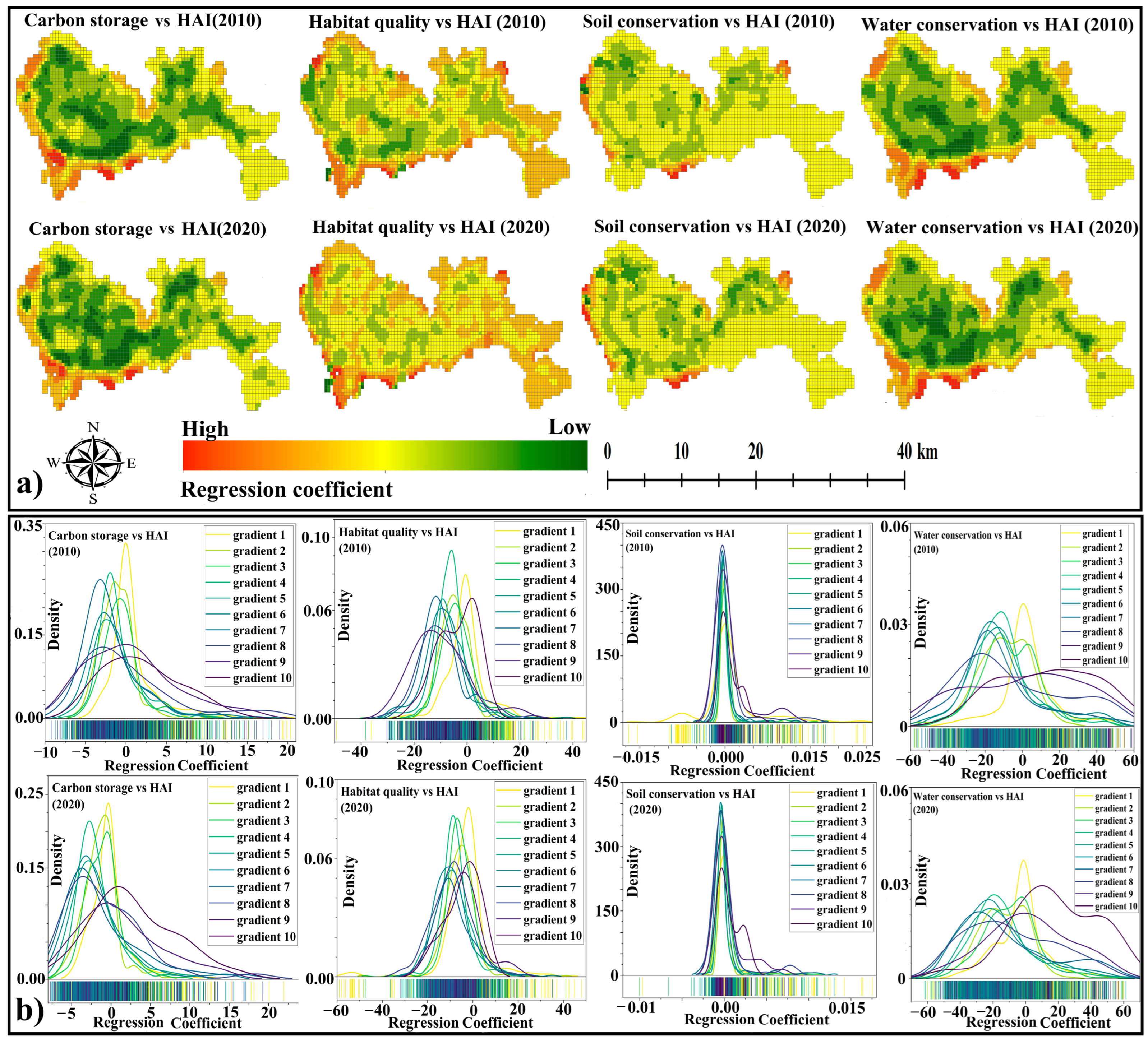
The influence of ESs on HAI and the trends in their effects varied regionally across gradient bands, with positive and negative “bidirectional” effects. In general, in 2010, the influence of ESs on HAI had a large negative driving effect, with the negative proportion of the regression coefficient reaching approximately 65%; then, the negative influence gradually increased in 2020, with the negative proportion of the regression coefficient reaching about 70%, and the scope of coverage was enlarged (Figure 9a). Among these, in 2010, the negative proportions of regression coefficients of carbon storage, soil conservation, water conservation, and habitat quality on HAI reached 64.91%, 64.61%, 65.69, and 78.29%, respectively; in 2020, the negative proportion of regression coefficients of carbon storage, soil conservation, water conservation, and habitat quality on HAI reached 72.78%, 68.73%, 72.35%, and 83.51%, respectively.

Figure 9.
Regression coefficients of HAI and ESs. (a) Spatial distribution of regression coefficients of ESs and HAI; (b) regression coefficients between ESs and HAI on different gradient bands.
In 2010 and 2020, the regression coefficients of ESs on HAI were somewhat different. The highest values of positive regression coefficients of carbon storage on HAI were 20.34 (2010) and 21.95 (2020), which were located in the first gradient band; the lowest values of negative regression coefficients were −9.23 (2010) and −7.67 (2020), which were located in the eighth gradient band. The highest values of positive regression coefficients of habitat quality on HAI were 59.91 (2010) and 47.99 (2020), and the lowest values of negative regression coefficients were −52.31 (2010) and −54.71 (2020), which were located on the first gradient band. The highest value of positive regression coefficients of water conservation on HAI were 50.21 (2010) and 51.04 (2020), which were located in the first gradient band, and the lowest values of negative regression coefficients were −67.31 (2010) and −69.73 (2020), which were located in the fourth and second gradient bands, respectively. The highest values of positive regression coefficients for soil conservation on HAI were 1.02 (2010) and 1.04 (2020), which were located in the first gradient band, and the lowest values of negative regression coefficients were −1.02 (2010) and −1.01 (2020), which were located in the seventh and third gradient bands, respectively (Figure 9b).
In summary, the positive relationships between ESs and HAI were mainly distributed in gradient bands 1–6, while the negative relationships were mainly distributed in gradient bands 1–8; the area covered by the negative relationships was larger than the area covered by the positive relationships in each gradient band. The highest span of regression coefficients between ESs and HAI was found in gradient band 1. This band contained the highest value of positive regression coefficients and the lowest value of negative regression coefficients, mainly because it was dominated by L-L and H-L agglomeration types. As the gradient increased, the regression coefficients on the second to seventh gradient bands shifted to negative values, and there were few positive regression coefficients, mainly because these gradient bands were gradually dominated by L-H and H-L. However, the fifth to seventh gradient bands had higher proportions of H-H. The regression coefficients for gradients 8 to 10 were shifted to positive values, mainly because the region was dominated by H-H and L-H agglomeration types (Figure 9a,b).
4. Discussion
4.1. Validation of ES Assessment Results
Currently, InVEST is used as an evaluation model to evaluate ESs; it has been widely used on various scales, and its scientificity and rationality have been verified [35,49]. Hence, this study used this model to carry out ES assessments. To further ensure the quality and accuracy of the ES assessment results, the NPP-based CASA model was selected for verifying the accuracy of the estimation results for water conservation, soil conservation, and habitat quality (ecosystem service diversity) [50,51]. In light of the different analysis results, we discuss the results from a spatial distribution perspective. The evaluation results of ESs in 2010 and 2020 were obtained using the InVEST model in this study. Among these results, water conservation was lower in the central and western regions, and higher in the southeast regions. Secondly, the spatial distribution of soil conservation in the east was significantly higher than that in the west, and was significantly higher in the south than in the north. Moreover, the distribution of biological mass gradually increased from the northwest to the southeast. This is basically in line with the research results of Chen et al. [52]. In summary, the resulting data regarding water conservation, soil conservation, and habitat quality in Shenzhen, as assessed using the CASA model, are similar to the spatial distribution results of high and low values of various ESs simulated using the model, indicating that the simulation results of ESs in the high-speed urbanization region obtained using various models are highly reliable. They can reflect the actual situation of ES changes [53]. The differences in values may be related to the spatial and temporal scales of the selected study area and the setting of model parameters. In addition, in terms of carbon sequestration, the parameters in the InVEST model of this study were determined by referring to the existing carbon density results of the Guangdong–Hong Kong–Macao Greater Bay Area [54]. To a certain extent, this also ensured the scientific results of this study.
4.2. Validation of HAI Results
Currently, the human footprint index method selects spatial data directly related to human activities (land use, population density, night lighting index, and road network data) for data preparation [19,20]. However, due to the differences in topography and regional development conditions in different regions, this method needs to be adjusted and optimized in different regions. Therefore, this study fully considered the economic and social development of the high-speed development area, and increased the density layer of urban facilities to represent the spatial distribution of HAI in the study area in 2010 and 2020. The areas with higher HAI were located in the western part of the study area, where various development and construction activities exist; meanwhile, the areas with lower HAI were located in the eastern part of the study area, which are mainly areas with higher vegetation cover. The results obtained in this study show that areas with a high level of economic development, low vegetation cover, and predominantly built-up land have high HAI, while areas with a low level of economic development, high vegetation cover, and nature reserves have low HAI. This is very similar to the results of Wang et al. [55] and Huang et al. [20]; to a certain extent, this proves the feasibility and scientificity of the human footprint index model constructed in this study.
In addition, a comparison was made between the various methods used to study the spatialization of HAI. From the point of view of methodological difficulties, the global disturbance index method is the simplest in that it directly uses MODIS product data, followed by the land type change method [56]; however, the global disturbance index method is only applicable to forested areas and can only evaluate the impacts of a few types of human activities, while the land type change method has obvious shortcomings in terms of the accuracy of the evaluation results [57]. From this point of view, the comprehensive index method is the best, followed by the human footprint index method [1], but data prepared using the comprehensive index method have obvious shortcomings in terms of spatial refinement and fineness [58]. In summary, we found that the human footprint index model is more suitable for the spatial quantification of HAI in terrestrial systems.
4.3. Exploring the Relationship between HAI and ESs
The scientific question regarding “the gradient response of HAI to ESs” originates from topographic gradients [59]. Based on existing studies, it has been shown that the qualities of an ecological environment, or its ESs, exhibit a certain regularity as the topographic gradient changes [60]. In addition, human activities are a central factor in ecological environment changes. With an increase in HAI, ESs are drastically perturbed. Moreover, there are significant spatial differences in the impacts of human activities on ESs, mainly negative impacts, which is similar to the results of Zhang et al. [36] and Sun et al. [2].
Currently, there are few studies on the gradient response between HAI and ESs and a lack of comparative exploration. In this study, the MGWR and bivariate spatial autocorrelation models [61] were introduced on the basis of gradient division results, and it was found that HAI is negatively correlated with ESs as the gradient changes. Firstly, from 2010 to 2020, the HAI in the study area showed a downward trend in the 1st–3th gradient bands and an upward trend in the 4th–10th gradient bands, indicating that the HAI region is advancing from a low-intensity region to a medium-intensity region. Secondly, in the low-intensity human activity regions (1st–3th gradient bands), the mean values of each ES were higher than the average level in the study area; as the gradient increased in the high-intensity human activity regions (6th–10th gradient bands), the mean values of each ES were at more similar levels. Thirdly, the L-L and H-L aggregation types are mainly distributed in the 1st–3rd gradient bands, while the H-H and L-H aggregation types are mainly distributed in the 6th gradient band, which is mainly because the ES levels in the 6th–10th gradient bands are closer to each other; the 6th gradient band is the area with a high intensity of human activities in which ESs reached a higher level. Finally, from the perspective of geospatial distribution, there were large spatial differences in the effects of ESs on HAI. In the first to third gradient bands, the absolute value of the regression coefficient of ESs on HAI was small, mainly because the region is dominated by forested land and other vegetated land. Such land is weakly affected by HAI, and the emphasis on green protection in ecological barrier areas has made the degree of influence of ESs on HAI in this region relatively stable. In the 6th to 10th gradient bands, the region is dominated by construction land, which is highly affected by HAI; the absolute value of the regression coefficient gradually increased, so that the negative effect of ES weakening, due to the increase in HAI, increased for this region. Therefore, to a certain extent, this shows that ESs can be maintained at a better level under the influence of a medium HAI level.
4.4. Measures Recommendations
In this rapidly developing region of China, frequent human activities affect the changes in the ecosystem’s structure, function, and services, resulting in an overall negative correlation between HAI and ESs [4]. Based on the distribution characteristics of ES changes along HAI gradients and on their functional relationships, corresponding suggestions have been put forward to alleviate the pressure of human activities on ecosystems and promote the sustainable development of highly urbanized areas [54,62]:
In the first to third gradient bands, the L-L and H-L types dominate. Of these, the L-L region should take ecological environment protection and restoration as its priority, avoid excessive development and construction activities, and promote the overall enhancement and optimization of ESs; the H-L region should continue to take ecological protection as its top priority, follow the principles of scientific planning, ecological priority, and strict protection, and pay attention to protecting ecological barrier areas and strengthening ecological financial support.
In the sixth gradient band, the region is dominated by H-H and L-H agglomeration types. Of these, the H-H region should pay attention to the advantages of high-speed economic development areas in terms of resources, should promote the construction of green spaces in neighboring areas, and should enrich urban ecosystem diversity; the L-H region should take into account ecological protection and resource utilization, optimize urban spatial layout, promote the efficient use of construction land, reduce the ecological land fragmentation caused by human over-development activities, and improve the intensive use of land.
In other gradient bands, HAI was negatively correlated with ESs as a whole. In terms of construction land, in these areas, more attention should be paid to the restoration of the ecological environment in terms of economic development; for non-construction land areas, we should reduce the damage to the urban ecological environment caused by human activities, and integrate the goals of urban economic development and environmental protection.
4.5. Limitations and Prospects
First of all, some of the parameters required by the InVEST model, for calculating water conservation, soil conservation, habitat quality, and carbon sequestration function, were obtained from previous studies, such as vegetation cover and crop management factors, soil conservation measures factors, etc. The values of the parameters in different regions may be slightly biased, which may have affected the calculation results. Secondly, in quantifying HAI, this study simply added up the indicators without considering the mutual influences between the various types of activities, resulting in potential uncertainty in the evaluation results. Meanwhile, this study selected six indicators with the help of spatial and temporal geographic data (e.g., night-time light remote sensing, POI, etc.), which, to a certain extent, satisfies scale unity for each indicator. However, the breadth and precision of data coverage are still urgent issues to be solved. Finally, HAI with different gradients has a bidirectional relationship with ESs. For example, rapid urbanization has a negative relationship with ESs, while ecological restoration projects improve habitat quality and have a positive relationship. However, in this study, only the bivariate spatial autocorrelation model and MGWR model were used to explore the action intensity and aggregation types of ESs and HAI at different gradients. This means that the bidirectional relationship between HAI and ESs may not be well reflected; such a problem could be the focus of future research.
After examining the shortcomings of existing studies, firstly, in future studies, the interactions between ESs and HAI should be analyzed through other relationship types besides spatial ones; additionally, the mechanism of influence of different HAI gradient changes on the interrelationships between different kinds of ES should be analyzed. Secondly, based on the human footprint index model and the InVEST model, data sources should be enriched, data accuracy should be improved, and the accuracy and precision of HAI and ES measurements should also be improved.
5. Conclusions
This study captured the HAI and ESs in the study area; 10 gradient bands of HAI were delineated using the average breakpoint method and additionally, the aggregation types and relationship between ESs and HAI were analyzed from a gradient perspective. Our study’s main conclusions are as follows:
- (1)
- From 2010 to 2020, the HAI not only exhibited an increasing trend in terms of numerical value, but the area of the high gradient band of HAI also showed an expanding trend, with an overall progression towards the southwest coast of the study area.
- (2)
- From 2010 to 2020, the carbon storage, habitat quality soil conservation, and water conservation showed relatively similar numerical changes in their trends; although the value fluctuation range was different, the change amplitude was the same. Secondly, the spatial distribution pattern of ESs was similar, showing a high distribution in the southeast and a low distribution in the west and middle regions.
- (3)
- In the low-intensity human activity regions (1st–3rd gradient bands), the mean values of each ES were higher than the average level in the study area; as the gradient increased, in the high-intensity human activity regions (6th–10th gradient bands), the mean values of each ES were at more similar levels. In addition, the ESs have a significant negative relationship with HAI, which is mainly concentrated in the 1st to 3rd gradient bands.
In conclusion, this study attempts to build a bridge between HAI and ESs from a gradient perspective. The research results are conducive to the fine management of high-speed urbanization areas, and can provide a basic reference for decision makers in implementing corresponding maintenance service function measures under different HAI gradients.
Author Contributions
Methodology, X.Z.; Formal analysis, Y.Y.; Investigation, X.Z.; Data curation, X.Z.; Writing—original draft, Y.Y.; Supervision, Y.Y.; Funding acquisition, Y.Y. All authors have read and agreed to the published version of the manuscript.
Funding
This research was financially supported by the Open Fund of Key Laboratory of Urban Land Resources Monitoring and Simulation, Ministry of Natural Resources (No. KF-2022-07-011), and the Youth Fund for Humanities and Social Sciences, Ministry of Education (No. 23YJC630212). The authors would extend appreciation to all the anonymous reviewers and editors for their constructive comments that improved this study.
Institutional Review Board Statement
Not applicable.
Informed Consent Statement
Not applicable.
Data Availability Statement
The data that support the findings of this study are available from the corresponding author upon reasonable request.
Conflicts of Interest
The authors declare no conflict of interest.
References
- Ai, M.; Chen, X.; Yu, Q. Spatial correlation analysis between human disturbance intensity (HDI) and ecosystem services value (ESV) in the Chengdu-Chongqing urban agglomeration. Ecol. Indic. 2024, 158, 111555. [Google Scholar] [CrossRef]
- Sun, Y.X.; Liu, S.L.; Shi, F.M.; An, Y.; Li, M.Q.; Liu, Y.X. Spatio-temporal variations and coupling of human activity intensity and ecosystem services based on the four-quadrant model on the Qinghai-Tibet Plateau. Sci. Total Environ. 2020, 743, 140721. [Google Scholar] [CrossRef]
- Costanza, R.; de Groot, R.; Sutton, P.; Ploeg, S.V.D.; Anderson, S.J.; Kubiszewski, I.; Farber, S.; Turner, R.K. Changes in the global value of ecosystem services. Glob. Environ. Chang. 2014, 26, 152–158. [Google Scholar] [CrossRef]
- Hou, Y.; Liu, Y.; Zeng, H. Assessment of urban ecosystem condition and ecosystem services in Shenzhen based on the MAES analysis framework. Ecol. Indic. 2023, 155, 110962. [Google Scholar] [CrossRef]
- Costanza, R. Valuing natural capital and ecosystem services toward the goals of efficiency, fairness, And sustainability. Ecosyst. Serv. 2020, 43, 101096. [Google Scholar] [CrossRef]
- Xie, Y.C.; Zhang, Y.; Luo, J.L.; Bi, L.Q.; Tong, K. Spatiotemporal heterogeneity and influencing factors of human activity intensity in the Guangxi Beibu Gulf Zone, China. Environ. Sustain. Indic. 2024, 22, 100372. [Google Scholar] [CrossRef]
- Anderson, C.B.; Seixas, C.S.; Barbosa, O.; Fennessy, M.S.; Herrera-F, B. Determining nature’s contributions to achieve the sustainable development goals. Sustain. Sci. 2019, 14, 543–547. [Google Scholar] [CrossRef]
- Aguilera, M.A.; Tapia, J.; Gallardo, C.; Núñez, P.; Varas-Belemmi, K. Loss of coastal ecosystem spatial connectivity and services by urbanization: Natural-to-urban integration for bay management. J. Environ. Manag. 2020, 276, 111297. [Google Scholar] [CrossRef]
- Amponsah, O.; Blija, D.K.; Ayambire, R.A.; Takyi, S.A.; Mensah, H.; Braimah, I. Global urban sprawl containment strategies and their implications for rapidly urbanising cities in Ghana. Land Use Policy 2022, 114, 105979. [Google Scholar] [CrossRef]
- Liu, H.; Fan, J.; Zhou, K.; Xu, X.; Zhang, H.; Guo, R.; Chen, S. Assessing the dynamics of human activity intensity and its natural and socioeconomic determinants in Qinghai–Tibet Plateau. Geogr. Sustain. 2023, 4, 294–304. [Google Scholar] [CrossRef]
- Casas-Ledón, Y.; Andrade, C.; Salazar, C.; Martínez-Martínez, Y.; Aguayo, M. Understanding the dynamics of human appropriation on ecosystems via an exergy-based net primary productivity indicator: A case study in south-central Chile. Ecol. Econ. 2023, 210, 107862. [Google Scholar] [CrossRef]
- Dai, X.; Yang, Y.; Zheng, H.; Meng, N.; Zhu, J.; Li, R.; Ma, J.; Lu, Z.; Li, Z. An integrated method to quantify human appropriation of net primary production in grasslands of the Qinghai-Tibet Plateau. Appl. Geogr. 2023, 158, 103055. [Google Scholar] [CrossRef]
- Kastner, T.; Matej, S.; Forrest, M.; Gingrich, S.; Haberl, H.; Hickler, T.; Krausmann, F.; Lasslop, G.; Niedertscheider, M.; Plutzar, C.; et al. Land use intensification increasingly drives the spatiotemporal patterns of the global human appropriation of net primary production in the last century. Glob. Chang. Biol. 2021, 28, 307–322. [Google Scholar] [CrossRef] [PubMed]
- Mildrexler, D.J.; Zhao, M.; Running, S.W. Testing a MODIS Global Disturbance Index across North America. Remote Sens. Environ. 2009, 113, 2103–2117. [Google Scholar] [CrossRef]
- Carrasco, J.; Acuna, M.; Miranda, A.; Alfaro, G.; Pais, C.; Weintraub, A. Exploring the multidimensional effects of human activity and land cover on fire occurrence for territorial planning. J. Environ. Manag. 2021, 297, 113428. [Google Scholar] [CrossRef] [PubMed]
- Zhang, X.; Xu, Z. Functional Coupling Degree and Human Activity Intensity of Production–Living–Ecological Space in Underdeveloped Regions in China: Case Study of Guizhou Province. Land 2021, 10, 56. [Google Scholar] [CrossRef]
- Zhang, X.; Ning, X.; Wang, H.; Zhang, X.; Liu, Y.; Zhang, W. Quantitative assessment of the risk of human activities on landscape fragmentation: A case study of Northeast China Tiger and Leopard National Park. Sci. Total Environ. 2022, 851, 158413. [Google Scholar] [CrossRef] [PubMed]
- Sanderson, E.W.; Jaiteh, M.; Levy, M.A.; Redford, K.H.; Wannebo, A.V.; Woolmer, G. The human footprint and the last of the wild. Bioscience 2002, 52, 891–904. [Google Scholar] [CrossRef]
- Liu, X.; Zhao, W.; Yao, Y.; Pereira, P. The rising human footprint in the Tibetan Plateau threatens the effectiveness of ecological restoration on vegetation growth. J. Environ. Manag. 2024, 351, 119963. [Google Scholar] [CrossRef]
- Huang, Z.; Chen, Y.; Zheng, Z.; Wu, Z. Spatiotemporal coupling analysis between human footprint and ecosystem service value in the highly urbanized Pearl River Delta urban Agglomeration, China. Ecol. Indic. 2023, 148, 110033. [Google Scholar] [CrossRef]
- Duan, H.T.; Luo, L.H. Summary and prospect of spatialization method of human activity intensity: Taking the Qinghai-Tibet Plateau as an example. J. Glaciol. Geocryol. 2021, 43, 1582–1593, (In Chinese with English Abstract). [Google Scholar]
- Hua, T.; Zhao, W.; Cherubini, F.; Hu, X.; Pereira, P. Continuous growth of human footprint risks compromising the benefits of protected areas on the Qinghai-Tibet Plateau. Glob. Ecol. Conserv. 2022, 34, e02053. [Google Scholar] [CrossRef]
- Costanza, R.; d’Arge, R.; de Groot, R.; Farber, S.; Grasso, M.; Hannon, B.; Limburg, K.; Naeem, S.; O’Neill, R.V.; Paruelo, J.; et al. The value of the world’s ecosystem services and natural capital. Nature 1997, 387, 253–260. [Google Scholar] [CrossRef]
- Ouyang, Z.Y.; Zhu, C.Q.; Yang, G.B.; Xu, W.H.; Xiao, Y. Gross ecosystem product: Concept, accounting framework and case study. Acta Ecol. Sin. 2013, 33, 6747–6761, (In Chinese with English Abstract). [Google Scholar] [CrossRef]
- Xie, G.D.; Zhang, C.X.; Zhang, L.M.; Chen, W.H.; Li, S.M. Improvement of the Evaluation Method for Ecosystem Service Value Based on Per Unit Area. J. Nat. Resour. 2015, 30, 123–1254, (In Chinese with English Abstract). [Google Scholar]
- MA (Millennium Ecosystem Assessment). Ecosystems and Human Well-Being: A Framework for Assessment; Island Press: Washington, DC, USA, 2003. [Google Scholar]
- United nations environmental program. Millennium Ecosystem Assessment Ecosystems and Human Wellbeing Synthesis; Island Press: Washington, DC, USA, 2005. [Google Scholar]
- Hou, L.; Wu, F.Q.; Xie, X.L. The spatial characteristics and relationships between landscape pattern and ecosystem service value along an urban-rural gradient in Xian city, China. Ecol. Indic. 2020, 108, 105720. [Google Scholar] [CrossRef]
- Yu, C.; Zhang, Z.; Jeppesen, E.; Gao, Y.; Liu, Y.; Lu, Q.; Wang, C.; Sun, X. Assessment of the effectiveness of China’s protected areas in enhancing ecosystem services. Ecosyst. Serv. 2024, 65, 101588. [Google Scholar] [CrossRef]
- Ren, Q.; Liu, D.D.; Liu, Y.F. Spatio-temporal variation of ecosystem services and the response to urbanization: Evidence based on Shandong province of China. Ecol. Indic. 2023, 151, 110333. [Google Scholar] [CrossRef]
- Fang, Z.; Ding, T.H.; Chen, J.Y.; Xue, S.; Zhou, Q.; Wang, Y.D.; Wang, Y.X.; Huang, Z.D.; Yang, S.L. Impacts of land use/land cover changes on ecosystem services in ecologically fragile regions. Sci. Total Environ. 2022, 831, 154967. [Google Scholar] [CrossRef]
- Yu, H.; Chen, C.; Shao, C.F. Spatial and temporal changes in ecosystem service driven by ecological compensation in the Xin’an River Basin, China. Ecol. Indic. 2023, 146, 109798. [Google Scholar] [CrossRef]
- Gong, J.; Jin, T.T.; Liu, D.Q. Are ecosystem service bundles useful for mountainous landscape function zoning and management? A case study of Bailongjiang watershed in western China. Ecol. Indic. 2022, 134, 108495. [Google Scholar] [CrossRef]
- Guo, C.Q.; Xu, X.B.; Sun, Q. A review on the assessment methods of supply and demand of ecosystem services. Chin. J. Ecol. 2020, 39, 2086–2096, (In Chinese with English Abstract). [Google Scholar]
- Cong, W.; Sun, X.; Guo, H.; Shan, R. Comparison of the SWAT and InVEST models to determine hydrological ecosystem service spatial patterns, priorities and trade-offs in a complex basin. Ecol. Indic. 2020, 112, 106089. [Google Scholar] [CrossRef]
- Zhang, X.; Zheng, Z.; Sun, S.; Wen, Y.; Chen, H. Study on the driving factors of ecosystem service value under the dual influence of natural environment and human activities. J. Clean. Prod. 2023, 420, 138408. [Google Scholar] [CrossRef]
- Xu, Z.H.; Wei, H.J.; Fan, W.G.; Wang, X.C.; Zhang, P.; Ren, J.H.; Lu, N.C.; Gao, Z.C.; Dong, X.B.; Kong, W.D. Relationships between ecosystem services and human well-being changes based on carbon flow—A case study of the Manas River Basin, Xinjiang, China. Ecosyst. Serv. 2019, 37, 100934. [Google Scholar] [CrossRef]
- Sun, Y.H.; Zhang, S.R.; Xu, Q.H. Pollen-based land cover changes reveal temporal and spatial differences of human activity in north-central China during the Holocene. Catena 2022, 219, 106620. [Google Scholar] [CrossRef]
- Qi, Y.; Lian, X.; Wang, H.; Zhang, J.; Yang, R. Dynamic mechanism between human activities and ecosystem services: A case study of Qinghai lake watershed, China. Ecol. Indic. 2020, 117, 106528. [Google Scholar] [CrossRef]
- Rong, Y.; Li, K.; Guo, J. Multi-scale spatio-temporal analysis of soil conservation service based on MGWR model: A case of Beijing-Tianjin-Hebei, China. Ecol. Indic. 2022, 139, 108946. [Google Scholar] [CrossRef]
- Fotheringham, A.S.; Yang, W.B.; Kang, W. Multiscale Geographically Weighted Regression (MGWR). Ann. Am. Assoc. Geogr. 2017, 107, 1247–1265. [Google Scholar] [CrossRef]
- Liu, X.; Su, Y.; Li, Z.; Zhang, S. Constructing ecological security patterns based on ecosystem services trade-offs and ecological sensitivity: A case study of Shenzhen metropolitan area, China. Ecol. Indic. 2023, 154, 110626. [Google Scholar] [CrossRef]
- Xu, C.; Jiang, W.Y.; Huang, Q.Y.; Wang, Y.T. Ecosystem services response to rural-urban transitions in coastal and island cities: A comparison between Shenzhen and Hong Kong, China. J. Clean. Prod. 2020, 260, 121033. [Google Scholar] [CrossRef]
- Sharp, R.; Chaplin-Kramer, R.; Wood, S.; Guerry, A.; Tallis, H.; Ricketts, T.; Nelson, E.; Ennaanay, D.; Wolny, S.; Olwero, N.; et al. InVEST User’s Guide; The Natural Capital Project, Stanford University, University of Minnesota, The Nature Conservancy, and World Wildlife Fund: Washington, DC, USA, 2018. [Google Scholar] [CrossRef]
- Zhang, X.R.; Zhou, J.; Li, G.N.; Chen, C.; Li, M.M.; Luo, J.M. Spatial pattern reconstruction of regional habitat quality based on the simulation of land use changes from 1975 To 2010. J. Geogr. Sci. 2020, 30, 601–620. [Google Scholar] [CrossRef]
- Zhao, Q.J.; Shao, J.F. Evaluating the impact of simulated land use changes under multiple scenarios on ecosystem services in Ji’an, China. Ecol. Indic. 2023, 156, 111040. [Google Scholar] [CrossRef]
- Cao, X.; Shi, Y.; Zhou, L.; Tao, T.; Yang, Q. Analysis of Factors Influencing the Urban Carrying Capacity of the Shanghai Metropolis Based on a Multiscale Geographically Weighted Regression (MGWR) Model. Land 2021, 10, 578. [Google Scholar] [CrossRef]
- Qiao, W.Y.; Huang, X.J. The impact of land urbanization on ecosystem health in the Yangtze River Delta urban agglomerations, China. Cities 2022, 130, 103981. [Google Scholar] [CrossRef]
- Mao, B.; Wang, X.; Liao, Z.; Miao, Y.; Yan, S. Spatiotemporal variations and tradeoff-synergy relations of ecosystem services under ecological water replenishment in Baiyangdian Lake, North China. J. Environ. Manage. 2023, 343, 118229. [Google Scholar] [CrossRef] [PubMed]
- Zhao, X.Q.; Shi, X.Q.; Li, Y.H.; Li, Y.M.; Huang, P. Spatio-temporal pattern and functional zoning of ecosystem services in the karst mountainous areas of southeastern Yunnan. Acta Geogr. Sin. 2022, 77, 736–756, (In Chinese with English Abstract). [Google Scholar] [CrossRef]
- Wu, Y.D.; Meng, J.J. Quantifying the spatial pattern for the importance of natural resource ecosystem services in China. J. Nat. Resour. 2022, 37, 17–33. [Google Scholar] [CrossRef]
- Chen, T.; Ye, Y.H.; Sun, F.F. Assessment on the Importance of Ecosystem Service Function in Shenzhen City Based on SPOT Data. Ecol. Econ. 2018, 34, 151–157, (In Chinese with English Abstract). [Google Scholar]
- Zhao, Y.; Wang, N.; Luo, Y.; He, H.; Wu, L.; Wang, H.; Wang, Q.; Wu, J. Quantification of ecosystem services supply-demand and the impact of demographic change on cultural services in Shenzhen, China. J. Environ. Manag. 2022, 304, 114280. [Google Scholar] [CrossRef]
- Wen, D.; Wang, X.; Liu, J.; Xu, N.; Zhou, W.; Hong, M. Maintaining key ecosystem services under multiple development scenarios: A case study in Guangdong–Hong Kong–Macao greater bay Area, China. Ecol. Indic. 2023, 154, 110691. [Google Scholar] [CrossRef]
- Wang, Z.; Liu, S.; Li, J.; Pan, C.; Wu, J.; Ran, J.; Su, Y. Remarkable improvement of ecosystem service values promoted by land use/land cover changes on the Yungui Plateau of China during 2001–2020. Ecol. Indic. 2022, 142, 109303. [Google Scholar] [CrossRef]
- Wu, W.; Yang, F.L.; Wang, J.J. Dynamic monitoring and analysis of ecosystem disturbances in major vegetation types based on MODIS time series data in Southwest China. Geogr. Res. 2021, 40, 1478–1494, (In Chinese with English Abstract). [Google Scholar]
- Chen, B.; Jing, X.; Liu, S.; Jiang, J.; Wang, Y. Intermediate human activities maximize dryland ecosystem services in the long-term land-use change: Evidence from the Sangong River watershed, northwest China. J. Environ. Manag. 2022, 319, 115708. [Google Scholar] [CrossRef] [PubMed]
- Yu, T.; Abulizi, A.; Xu, Z.; Jiang, J.; Akbar, A.; Ou, B.; Xu, F. Evolution of environmental quality and its response to human disturbances of the urban agglomeration in the northern slope of the Tianshan Mountains. Ecol. Indic. 2023, 153, 110481. [Google Scholar] [CrossRef]
- Li, M.; Luo, G.; Li, Y.; Qin, Y.; Huang, J.; Liao, J. Effects of landscape patterns and their changes on ecosystem health under different topographic gradients: A case study of the Miaoling Mountains in southern China. Ecol. Indic. 2023, 154, 110796. [Google Scholar] [CrossRef]
- Sannigrahi, S.; Zhang, Q.; Pilla, F.; Joshi, P.K.; Basu, B.; Keesstra, S.; Roy, P.S.; Wang, Y.; Sutton, P.C.; Chakraborti, S.; et al. Responses of ecosystem services to natural and anthropogenic forcings: A spatial regression based assessment in the world’s largest mangrove ecosystem. Sci. Total Environ. 2020, 715, 137004. [Google Scholar] [CrossRef] [PubMed]
- Yan, G.; Wang, S. Coexistence and transformation from urban industrial land to green space in decentralization of megacities: A case study of Daxing District, Beijing, China. Ecol. Indic. 2023, 156, 111120. [Google Scholar] [CrossRef]
- Zhang, X.; Chen, D.C.; Fan, J.D.; Yu, C.; Zhou, Y.; Tang, J.J. Study on the change of ecosystem service value and its correlation with human activities: Taking Changzhou City as an example. J. Environ. Eng. Technol. 2022, 12, 2124–2131, (In Chinese with English Abstract). [Google Scholar]
Disclaimer/Publisher’s Note: The statements, opinions and data contained in all publications are solely those of the individual author(s) and contributor(s) and not of MDPI and/or the editor(s). MDPI and/or the editor(s) disclaim responsibility for any injury to people or property resulting from any ideas, methods, instructions or products referred to in the content. |
© 2024 by the authors. Licensee MDPI, Basel, Switzerland. This article is an open access article distributed under the terms and conditions of the Creative Commons Attribution (CC BY) license (https://creativecommons.org/licenses/by/4.0/).