Spatio-Temporal Variation Analysis of Soil Salinization in the Ougan-Kuqa River Oasis of China

Abstract

In order to investigate the mechanism of environmental factors in soil salinization, this study focused on analyzing the temporal-spatial variation of soil salinity in the Ogan-Kuqa River Oasis in Xinjiang, China. The research aimed to predict soil salinity using a combination of satellite data, environmental covariates, and advanced modeling techniques. Firstly, Boruta and ReliefF algorithms were employed to select variables that significantly affect soil salinity from the Sentinel-2 satellite data and environmental covariates. Subsequently, a soil salinity inversion model was established using three advanced strategies: comprehensive variable analysis, a Boruta-based variable selection algorithm, and a ReliefF-based variable selection algorithm. Each strategy was modeled using a Light Gradient Boosting Machine (LightGBM), an Extreme Learning Machine (ELM), and a Support Vector Machine (SVM). Finally, the Boruta-LightGBM strategy was proven to be the most effective in predicting soil electrical conductivity (EC), with a coefficient of determination ($R^2$) of 0.72 and a Root Mean Square Error (RMSE) of 12.49 ds/m. The experimental results show that the red-edge band index is the foremost variable in predicting soil salinity, succeeded by the salinity index and soil attribute data, while the topographic index has the least influence, which further demonstrates that proper variable selection could significantly improve model functionality and predictive precision. Furthermore, the Multiscale Geographically Weighted Regression (MGWR) model was utilized to reveal the influence and temporal-temporal-spatial heterogeneity of environmental factors such as soil organic carbon (SOC), precipitation (PRE), pH value, and temperature (TEM) on soil EC. This research offers not just a viable methodological framework for monitoring soil salinization but also new perspectives on the environmental drivers of soil salinity changes, which have implications for sustainable land management and provide valuable information for decision-making in soil salinity control and mitigation efforts.

1. Introduction

Soil salinization is one of the gravest forms of land degradation worldwide, exerting significant effects on both the environment and agriculture. This phenomenon results in the considerable worsening of soil’s physical and chemical properties, a reduction in biodiversity, and a decrease in crop yields, sometimes even leading to plant death [1]. Hence, soil salinization is not just a topic of global research interest but also poses an immediate challenge to environmental protection and sustainable agriculture [2]. The accumulation of soil salinity is especially noticeable in arid and semi-arid areas, primarily caused by high evaporation and temperature levels. The accumulation of salts impacts the efficient provision of soil moisture and nutrients and further intensifies the extent of soil salinization [3]. Thus, employing remote sensing techniques to detect soil salinity and investigating its impact factors and temporal-spatial heterogeneity are vital for effectively managing and rehabilitating salinized soils, preventing their further deterioration, and sensibly using salinized soil resources, all of which are significant for sustaining the ecological development of salinized soils.

Spectral features are the core of soil salinity monitoring, where reflectance variations are directly associated with rising salinity levels [4]. Nonetheless, soil salinity monitoring based solely on optical remote sensing data is not always precise due to the influence of numerous factors such as vegetation, soil type, terrain, climate conditions, and human activities [5]. The intricate interactions among these factors mean that relying only on individual spectral characteristics cannot comprehensively disclose the spatial distribution of soil salinization. To surmount this challenge, the efficacy of digital mapping of soil salinity must depend on the combined use of multiple environmental covariates [6]. Zain et al. [7] evaluated several research areas according to key geotechnical characteristics in the Lahore metropolitan area based on IDW interpolation technology, which is based on the improved Shephard method that can efficiently generate very accurate geotechnical engineering soil maps. Ijaz et al. [8] used spatial interpolation technology to create a spatial map (SM) in the Sialkot area based on a large amount of geotechnical foundation data, and used linear regression analysis to establish the correlation, so that soil strength, stiffness, and soil consistency can be quickly and reliably evaluated. These covariates often display a continuous spatial distribution, so their relative significance must be taken into account during selection. Prior research has substantiated the significance of variable selection in improving the precision of model inversion [9,10,11,12]. Feature selection algorithms can automatically screen out the features that have an important impact on soil salinity. In addition, it can also be integrated with satellite remote sensing data, ground observation data, and environmental factor data. In order to accurately estimate soil salinity, Mohamed et al. [13] used the joint data to predict soil salinity and used the BPNN to select features that can help farmers in areas affected by soil salinization to better manage planting procedures and improve their land quality. Wang et al. [14] used the CNN and SVM to predict soil salinity, which shows that the models have great potential for measuring. In light of this, feature selection algorithms emerge as a vital tool for identifying and choosing critical environmental covariates with a significant impact on salinity. This method enables us to not only better comprehend the significant factors within the data but also to provide a more thorough and accurate integrated evaluation of soil salinity.

The relationship between the spatio-temporal distribution of soil salinity and a multitude of environmental factors is highly intricate [15]. In order to thoroughly comprehend these complex relationships, this study emphasizes examining the spatio-temporal non-stationarity characteristics, aiming to elucidate the influence degree and spatial variation of different factors on soil salinity. Geographically Weighted Regression (GWR) has been extensively applied in spatial modeling of soil attributes, exhibiting notable accuracy [16,17]. The main strength of this model lies in uncovering the spatio-temporal non-stationarity [18]. GWR integrates spatial location factors into regression parameters, permitting the weighting of each data point in the regression based on its proximity, meaning that the nearer points are assigned greater weight [19]. Yet, the conventional GWR model presumes that the optimal bandwidth for all influencing factors is consistent, which hinders the precise depiction of the real spatial processes of soil salinity [20]. In response to this constraint, Fotheringham and others developed the Multi-scale Geographically Weighted Regression (MGWR) model [21]. This model allocates distinct spatial smoothing levels to each variable, effectively surmounting the single bandwidth limitation of traditional GWR models and aligning more accurately with real spatial processes.

The main innovations of our paper are detailed as follows:

(1)

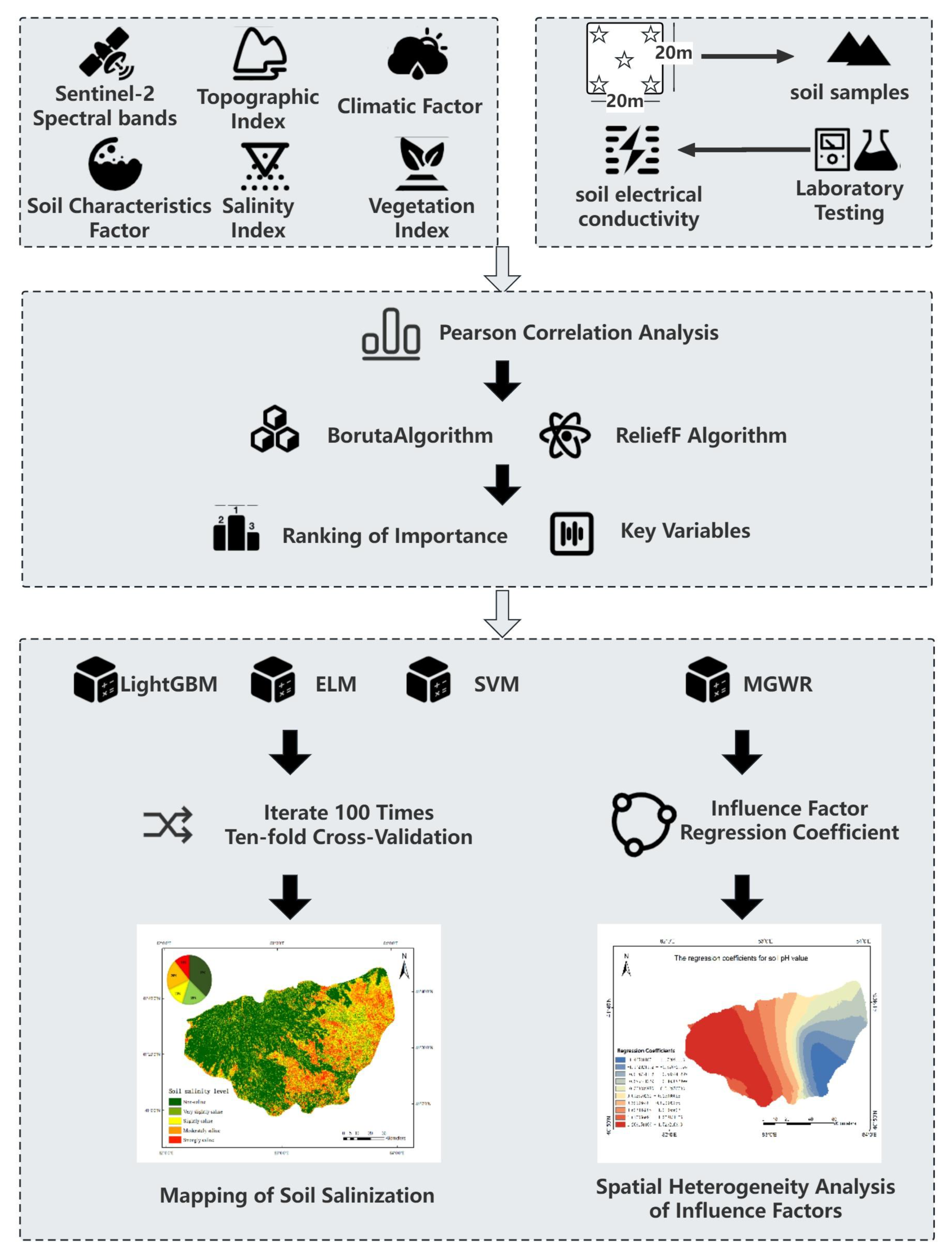
A new approach has been developed to combine spectral indices and various environmental covariates such as meteorology, terrain data, and soil attributes, with the aim of enhancing the accuracy and reliability of soil salinity monitoring.

(2)

The Boruta and ReliefF algorithms are employed to improve the feature selection process by reducing its complexity, thereby significantly enhancing the functionality and predictive accuracy of the models.

(3)

Based on the selected features, LightGBM, ELM, and SVM methods are employed to develop soil salinity inversion models to assess the influence of diverse input variables and modeling approaches on the accuracy of the salinity inversion models and to subsequently generate a map depicting the distribution of soil electrical conductivity in the Ogan-Kuqa River Oasis, Xinjiang, China.

(4)

The Multiscale Geographically Weighted Regression model (MGWR) is employed to examine the temporal-spatial variability of environmental factors impacting soil salinity, which contributes to a more thorough comprehension of the temporal-spatial distribution patterns of soil salinity and the complex dynamics of soil salinization influenced by a variety of environmental factors.

2. Materials and Methods

The workflow of this research is illustrated in Figure 1. First of all, summarize relevant index data such as Sentinel-2 data, topographical index, climate factors, soil characteristic factors, salinization factors, vegetation indices, etc. Secondly, collect soil samples in the study area and send them to the laboratory for testing and analysis, and predict the soil conductivity of the samples. Then, Pearson correlation analysis is carried out on the research results, the Boruta and ReliefF algorithms are used to divide and select features, and the importance of key variables is ranked and selected. Finally, based on the selected characteristic variables, models such as LightGBM, ELM, SVM, and MGWR are used to predict soil conductivity. Through 100 iterations and ten-fold cross-validation and regression analysis, land salinization mapping and spatial heterogeneity analysis of influencing factors of soil salinization are completed. Subsequent chapters will provide detailed explanations of these specific details.

2.1. Study Area and Data Acquisition

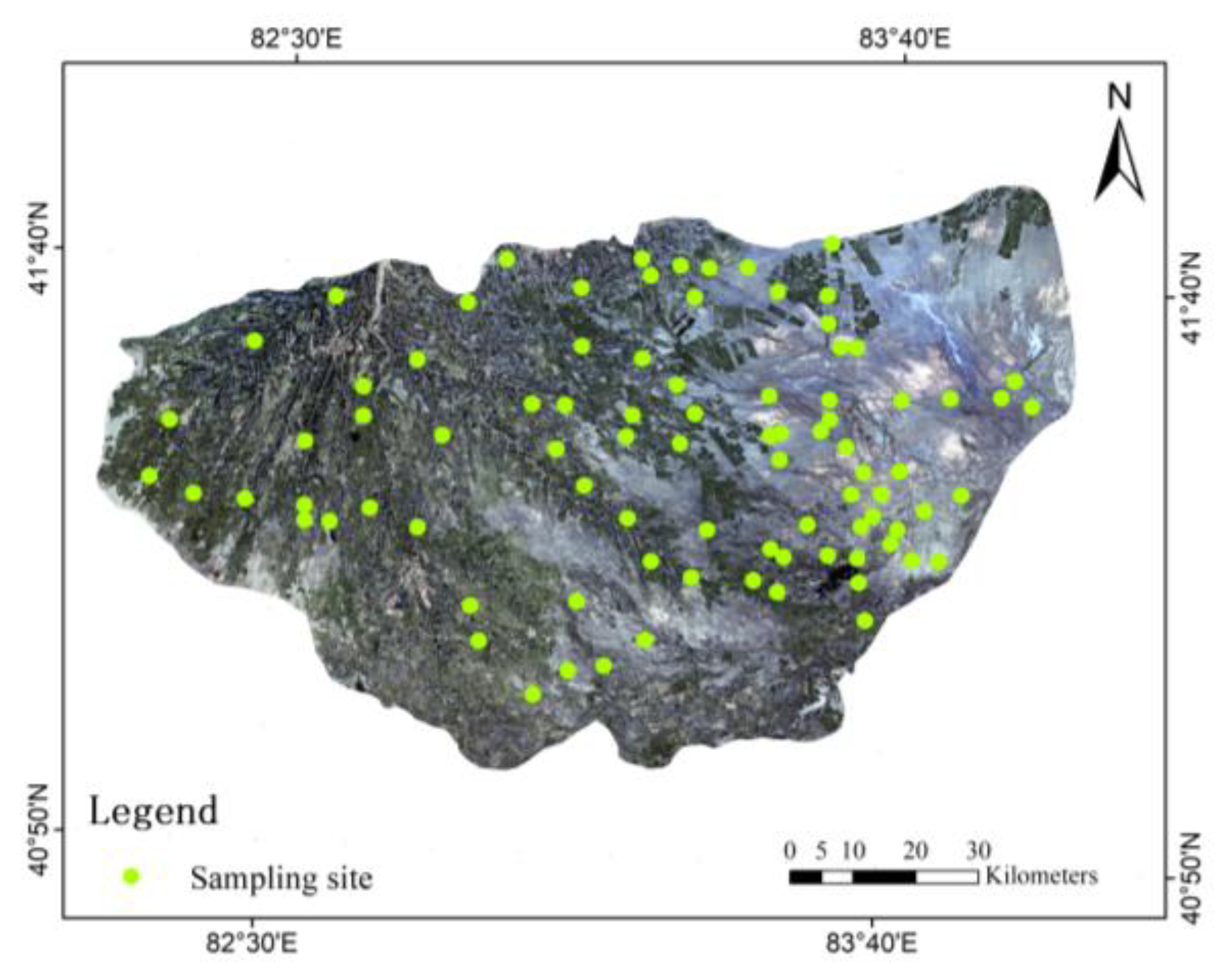
2.1.1. Study Area

The Ogan-Kuqa River Oasis in Xinjiang, China, situated on the northern fringe of the Tarim Basin and the southern slopes of the Tian Shan Mountains, borders the Taklamakan Desert, the second-largest mobile sand desert in the world. The Kuqa and Ogan Rivers flow through this oasis, with the Tarim River basin running through its southern section [22]. This region encompasses Kuqa City, Shayar County, and Xinhe County in the Aksu region, with a total area of approximately 9400 km² (Figure 2a). The geography is elevated in the northwest and descends towards the southeast, with elevations between 927 and 1065 m, generally exhibiting a flat landscape (Figure 2b). This oasis represents a classic inland arid region, falling under a continental warm temperate dry climate. The climate is arid with scant rainfall and notable temperature fluctuations. The extreme maximum temperature can soar to 41.6 °C, and the extreme minimum can plummet to −28.7 °C. It has an average annual precipitation of approximately 55.45 mm and an evaporation rate of 2356 mm, resulting in an evaporation-to-precipitation ratio as high as 43:1 [23]. Yet, in the oasis areas of Xinjiang, aiming for increased crop production and economic gains, local farmers frequently irrigate on unsuitable saline-alkali soils. This practice not only results in groundwater contamination to varying extents but also aggravates environmental problems such as soil salinization and the lowering of groundwater tables. This has led to soil salinization becoming a critical factor in the limiting of agricultural development in the area.

2.1.2. Soil Sampling and Analysis

Between 25 June and 2 July 2022, we developed a survey route and chose representative soil sampling sites for on-site investigations. In each sampling site, soil samples from 0–10 cm depth were gathered using the five-point sampling method, and we recorded their geographical coordinates, elevation, land cover types, and crops. Following air-drying, every 20 g of soil was combined with 100 mL of distilled water, and soil electrical conductivity (EC) was measured at 25 °C using a composite electrode. In total, 94 actual measurement sites were acquired. The distribution of these sampling sites is illustrated in Figure 3.

2.1.3. Acquisition and Pre-Processing of Remote Sensing Data

For this research, adhering to the principles of closeness to the sampling time and minimal cloudiness, we downloaded the Sentinel-2 Level-1C product’s imagery from 28 June 2022, with cloud cover under 20% and UTM/WGS84 coordinate projection, from ESA’s Copernicus Open Access Hub (https://scihub.copernicus.eu/, accessed on 8 December 2023). Atmospheric correction of the Sentinel-2 Level-1C data was conducted using the Sen2Cor tool (version 2.8), yielding Sentinel-2 Level-2A images (referred to as Sentinel-2 data henceforth).

The red-edge band index is the reflectivity of a narrow band between visible light and the near-infrared band, which is related to the photosynthesis intensity of vegetation. However, soil salinity will have a negative impact on the growth and photosynthesis of vegetation, leading to a decrease in the red band index, which has high sensitivity and responsiveness in the prediction of soil salinity. In addition, the red band index has high spatial resolution and repeatability and can be used to monitor soil salinity in a wide range through remote sensing technology, which has high practical value, so it is determined to be the primary variable in predicting soil salinity. After atmospheric correction, the bands were resampled to 20 m resolution by using the nearest neighbor approach before being fused and cropped using ENVI 5.3 software. Nine bands, B2, B3, B4, B5, B6, B7, B8, B11, and B12, were chosen, as shown in

Table 1. Introduction to band information.

Band	Description	Central Wavelength (nm)	Resolution (m)
band2	blue	490	10 m
band3	green	560	10 m
Band4	red	665	10 m
Band5	Red edg1	705	20 m
Band6	Red edg2	740	20 m
Band7	Red edg3	783	20 m
Band8	Near-infrared	842	10 m
Band11	Short wave infraed1	1610	20 m
Band12	Short wave infraed2	2190	20 m

.

2.1.4. Environmental Covariates

This research incorporates environmental covariates consisting of vegetation, terrain, climate, and fundamental soil characteristics. The indices for soil salinity and vegetation are derived from Sentinel-2 data. The foundational soil property data, encompassing soil organic carbon, pH levels, bulk density, and cation exchange capacity, originate from the Resource and Environmental Science and Data Center (http://www.resdc.cn, accessed on 8 December 2023). Topographical data are obtained using ASTER GDEM V2, provided by the Geospatial Data Cloud (http://www.gscloud.cn/, accessed on 8 December 2023). Moreover, nine terrain indices were computed by employing the Automated Geoscientific Analysis GIS (SAGA GIS). Climate-related environmental covariates, including monthly average temperature, precipitation, and potential evapotranspiration, are acquired from the National Tibetan Plateau Data Center (https://data.tpdc.ac.cn/, accessed on 8 December 2023). Monthly dryness is determined by the ratio of monthly potential evapotranspiration to average monthly precipitation. Using the nearest neighbor approach, the data mentioned above were resampled to a 20 m spatial resolution. The spectral index, formulas, and corresponding references are displayed in

Table 2. Introduction to spectral index.

Auxiliary	Spectral Index	Acronym	Formula	Reference
Vegetation Index	Normalized Difference Vegetation Index	NDVI	$NDVI=\frac{(NIR-R)}{(NIR+R)}$	[24]
	Enhanced Normalized Difference Vegetation Index	ENDVI	$ENDVI=\frac{(NIR+SWIR2-R)}{(NIR+SWIR2+R)}$	[24]
	Enhanced Vegetation Index	EVI	$EVI=2.5\times \frac{(NIR-R)}{(NIR+6\times R-7.5\times B+1)}$	[24]
	Extended Enhanced Vegetation Index	EEVI	$EVI=2.5\times \frac{(NIR+SWIR1)}{(NIR+SWIR1+6\times R-7.5\times B+1)}$	[24]
	Soil-Adjusted Vegetation Index	SAVI	$SAVI=(1+L)\times \frac{(NIR-R)}{(NIR+R+L)}$	[24]
	Modified Soil-Adjusted Vegetation Index	MSAVI	$MSAVI=\frac{\left(2\times NIR-1\right)-\sqrt{{\left(2\times NIR+1\right)}^2-8\times (NIR-R)}}{2}$	[24]
	Generalized Difference Vegetation Index	GDVI	$GDVI=\frac{({NIR}^2-R^2)}{({NIR}^2+R^2)}$	[24]
Salinity Index	Salinity Index	SI	$SI=\sqrt{B\times R}$	[24]
	Salinity Index 1	SI1	$SI1=\sqrt{G\times R}$	[24]
	Salinity Index 2	SI2	$SI2=\sqrt{G^2\times R^2+{NIR}^2}$	[24]
	Canopy Response Salinity Index	CRSI	$CRSI=\sqrt{\frac{(NIR\times R-G\times R)}{(NIR\times R+G\times R)}}$	[24]
	Normalized Difference Salinity Index	NDSI	$NDSI=\frac{(R-NIR)}{(R+NIR)}$	[24]
	Gypsum Index	GYEX	$GYEX=\frac{(SWIR1-NIR)}{(SWIR1+NIR)}$	[25]
	Clay Index	CLEX	$CLEX=\frac{SWIR1}{SWIR2}$	[25]
Red-Edge Band Index	Red edg1 NDSI	NDSIre1	$NDSIre1=\frac{(redE1-NIR)}{(redE1+NIR)}$	[26]
	Red edg2 NDSI	NDSIre2	$NDSIre2=\frac{(redE2-NIR)}{(redE2+NIR)}$	[26]
	Red edg3 NDSI	NDSIre3	$NDSIre3=\frac{(redE3-NIR)}{(redE3+NIR)}$	[26]
	Red edg1 DVI	DVIre1	$DVIre1=NIR-redE1$	[26]
	Red edg2 DVI	DVIre2	$DVIre2=NIR-redE2$	[26]
	Red edg3 DVI	DVIre3	$DVIre3=NIR-redE3$	[26]
	Red edg1 EVI	EVIre1	$2.5(NIR-redE1)/(NIR1+6 redE1-7.5B+1)$	[26]
	Red edg2 EVI	EVIre2	$2.5(NIR-redE2)/(NIR1+6 redE2-7.5B+1)$	[26]
	Red edg3 EVI	EVIre3	$2.5(NIR-redE3)/(NIR1+6 redE3-7.5B+1)$	[26]

, and the environmental covariates are displayed in

Table 3. Introduction to environmental covariates.

Auxiliary	Environmental Covariates	Acronym	Reference
Topographic Index	Digital Elevation Model	DEM	SAGA GIS
	Slope	Slope
	Aspect	Aspect
	Topographic Wetness Index	TWI
	Valley Depth	VD
	Stream Power Index	SPI
	Plan Curvature	PC
	Relative Slope Position	RSP
	Topographic Position Index	TPI
Climatic Factor	Monthly Average Precipitation	PRE	[27]
	Monthly Average Temperature	TEM	[28]
	Monthly Average Potential Evapotranspiration	PET	[28]
	Drought Index	R	[28]
Soil Characteristics Factor	Soil Organic Carbon	SOC	[22]
	pH Value	PH	[22]
	Cation Exchange Capacity	CEC	[22]
	Bulk Density	BD	[22]

.

2.2. Covariate Selection Algorithm

2.2.1. Boruta

Introduced by Miron B. Kursa and Witold R. Rudnicki [29], the Boruta method is an advanced method of feature selection, designed to overcome the uncertainties and subjective biases prevalent in conventional feature selection techniques. Based on the random forest algorithm, this method evaluates the importance of each feature by generating shadow features, which are random replicas of the original data attributes. In this process, Boruta iteratively contrasts all original and shadow features to accurately segregate those that significantly contribute to the predictive model from the insignificant ones [30]. The Boruta algorithm employs shadow features and characteristics of the binomial distribution as benchmarks for deciding the threshold of importance. Boruta’s primary advantage over traditional threshold-based feature selection methods is its comprehensive evaluation of feature importance, mitigating the risk of overlooking potentially critical features due to subjectively determined thresholds. This method, grounded in statistics, provides a more objective and holistic mechanism for feature selection, making it particularly effective for tackling issues of feature redundancy and correlation in high-dimensional data [31]. In our research, the Boruta algorithm was utilized for selecting features in the soil salinity monitoring model. This method was chosen for its ability to efficiently identify environmental covariates closely associated with changes in soil salinity, with the expectation of improving both the accuracy and robustness of our model. The application of the Boruta algorithm aims to deepen our understanding of the factors driving soil salinity changes, thereby offering more precise data support for soil salinity monitoring in Xinjiang, China. The Boruta algorithm is implemented by importing the BorutaPy module from the “Boruta” library within the Python 3.10 environment.

2.2.2. ReliefF

Since its inception in 1992 by Kira and Rendell, the ReliefF algorithm, a notable method for feature selection, has gained extensive application in machine learning and data analytics [32]. The core of ReliefF is to evaluate the capacity of each feature to distinguish between similar samples. ReliefF operates by randomly selecting samples and then examining the nearest similar (neighbor) and dissimilar samples, determining each feature’s contribution to the correct classification of the samples. Features are deemed important based on their ability to distinguish neighboring samples, particularly those that effectively differentiate between various categories [33]. ReliefF’s principal advantage over other feature selection techniques is its robustness against noise and irrelevant features in data, along with its ability to manage different data types, including both discrete and continuous features. Additionally, it excels in handling features with complex interrelationships. In our research, we employed the ReliefF algorithm for selecting features intimately connected with soil salinity monitoring. The choice is grounded in its exceptional capability to manage multidimensional and intricate environmental datasets, with the expectation of considerably improving the predictive accuracy and interpretability of our model. Utilizing this approach, our goal is to pinpoint the environmental covariates that most significantly impact soil salinization, thus offering data support for devising more effective soil management strategies.

2.3. Model Construction and Accuracy Evaluation

For this research, to evaluate the influence of various input variables on the accuracy of the model, we ensured consistency in the settings of parameters. Utilizing this method, we can more precisely ascertain the function and importance of different environmental covariates in the soil salinity forecasting model.

2.3.1. LightGBM

LightGBM, developed by Mahsa et al. in 2017, represents an efficient variation of the distributed Gradient-Boosting Decision Tree (GBDT) algorithm [34]. This algorithm utilizes a histogram-based approach for decision tree learning, focusing on improving both the training efficiency and predictive accuracy of the model. Operating within the gradient boosting framework, LightGBM bolsters model performance by training a series of decision tree ensembles. In its training phase, LightGBM continuously refines each decision tree’s learning objectives using the gradient information of loss function, amalgamating them into an effective ensemble model [35]. LightGBM innovates in two critical aspects relative to traditional GBDT models: firstly, by employing a LEAFWISE growth strategy that progresses at the level of leaf nodes, as opposed to the conventional depth-based priority splitting. This approach reduces the frequency of decision tree splits, thereby enhancing training efficiency. Secondly, it incorporates a histogram algorithm that categorizes the dataset into bins based on feature values, using these histograms to facilitate decision tree learning [36]. Moreover, LightGBM employs numerous optimization techniques, including feature parallel learning and histogram-aware split ordering, to further augment training speed and enhance model performance.

2.3.2. Extreme Learning Machine

First introduced in 2006 by Huang Guang-Bin and colleagues, the Extreme Learning Machine (ELM) has emerged as an important technique in the machine learning domain [37]. ELM, a learning algorithm for Single-Layer Feedforward Neural Networks (SLFNs), is distinguished by the random generation of weights and biases for hidden layer nodes, bypassing adjustments via backpropagation [38]. The unique training mechanism of ELM affords a substantially faster training speed than that of conventional neural networks. The key strengths of ELM lie in its exceptional generalization ability and rapid learning rate, particularly beneficial for managing large-scale datasets. Since its training does not rely on iterative optimization, ELM effectively avoids the local minima issue typically found in traditional neural network training. Moreover, ELM exhibits considerable adaptability to different types of data, encompassing both non-linear and high-dimensional data. The ELM algorithm swiftly conducts the training process by randomly initializing the hidden layer weights and biases, and employing straightforward, rapid computational techniques [39]. In detail, ELM employs weights and biases with random initial values as inputs to the hidden layer, processes input data using these weights and biases, and conveys the results to the output layer through an activation function. Output layer weights are calculated using a formulaic method aimed at minimizing predictive errors.

2.3.3. Support Vector Machine

The Support Vector Machine (SVM) is a robust algorithm proposed by Vapnik and Cortes [40]. Its fundamental concept involves identifying an optimal hyperplane within the feature space to optimally segregate data. The hyperplane is constructed to maximize the margin between diverse data categories, offering distinct classification decision rules [41]. The distinctiveness of the SVM algorithm is its ability to manage high-dimensional data and its exceptional performance with small sample sizes. Utilizing kernel methods, the SVM effectively tackles non-linear issues by mapping the original feature space into a higher-dimensional one, where it accomplishes linear separation. This methodology grants the SVM considerable flexibility and precision in dealing with intricate datasets.

2.3.4. Accuracy Evaluation

In this research, to manage potential fluctuations in model performance and guarantee the stability of the model predictions, ten-fold cross-validation is performed on the model, with each model undergoing 100 iterations. The validation accuracy of the model is evaluated using the coefficient of determination ($R^2$), root mean square error (RMSE), and mean absolute error (MAE). The closer $R^2$ is to 1, and the lower the RMSE and MAE, the better the predictive performance of the model.

$$R^2=1-\frac{\sum _{i=1}^n{(y_i-{\widehat{y}}_i)}^2}{\sum _{i=1}^n{(y_i-\overline{y})}^2}$$

(1)

$$\mathrm{R}\mathrm{M}\mathrm{S}\mathrm{E}=\sqrt{\frac{1}{n}{\sum }_{i=1}^n\left({(y_i-{\widehat{y}}_i)}^2\right)}$$

(2)

$$\mathrm{M}\mathrm{A}\mathrm{E}=\frac{1}{n}{\sum }_{i=1}^n\left|y_i-{\widehat{y}}_i\right|$$

(3)

In this equation, $n$ denotes the number of samples, $y_i$ represents the actual measured value of the sample, and ${\widehat{y}}_i$ is the predicted value of the sample.

2.4. Multiscale Geographically Weighted Regression

Multiscale Geographically Weighted Regression (MGWR) is applicable for scenarios involving spatial data with characteristics that vary across multiple scales [42]. MGWR operates by partitioning the dataset into various spatial sub-regions and employing the Geographically Weighted Regression (GWR) model within each to detect spatial non-stationarity and heterogeneity across diverse scales. Within MGWR, the regression model is constructed as the relationship between dependent and independent variables, where each scale possesses distinct regression coefficients. The mathematical expression for MGWR is as follows:

$$y_i={\beta }_0(u_i,v_i)+{\sum }_{i=1}^n{\beta }_{bwj}(u_i,v_i)\ast x_{ij}+{\epsilon }_i$$

(4)

In this equation, $(u_i,v_i)$ denotes the spatial coordinates of the i-th sample point; $y_i$ and $x_{ij}$ represent the values of the dependent and independent variables at position i; ${\beta }_0(u_i,v_i)$ is the constant term at the spatial position $(u_i,v_i)$; ${\epsilon }_i$ is a random error term, and ${\beta }_{bwj}(u_i,v_i)$ is the regression coefficient of the j-th independent variable at the spatial position i, fitted with a specific bandwidth bwj.

To mitigate multicollinearity impact on MGWR model results, tolerance and the Variance Inflation Factor (VIF) are employed as metrics to determine collinearity among factors, excluding explanatory variables with collinearity [43]. The smaller the tolerance, the more an explanatory variable is explained by other variables in the regression analysis, indicating potential severe collinearity problems. A rational tolerance range is between (0.1, +∞). A VIF value of ≥10 suggests the potential for significant collinearity among explanatory variables. When the VIF value lies between 1 and 10, it is inferred that the explanatory variables are free from multicollinearity.

In this research, the MGWR model will be utilized to construct a regression model for environmental variables, acquiring regression coefficients at every spatial position, to examine the spatial differences in the environmental variables’ influence on soil conductivity. Furthermore, in order to explore the scalability of the MGWR model, it is employed in other areas in Xinjiang, China, where it can deeply analyze the environmental factors and reveal the potential impact of environmental factors such as soil organic carbon, precipitation, pH value, and temperature in different geographical backgrounds or climates, thus enhancing the applicability of the MGWR model.

3. Results

3.1. Descriptive Statistics of Soil EC

The descriptive statistics for soil EC are presented in

Table 4. Descriptive statistics of the soil EC data.

EC Sample Data	Min	Max	Mean	SD	CV
whole data (n = 94)	0.17	90.30	20.63	23.85	1.16

. Soil electrical conductivity (EC) ranges from 0.17 to 90.3 dS m⁻¹, averaging 20.63 dS m⁻¹. The standard deviation and coefficient of variation are, respectively, 23.85 dS m⁻¹ and 1.16. The high standard deviation and coefficient of variation suggest a diffusion trend in the surface soil salinity of the Ogan-Kuqa River Oasis area, indicative of strong variability.

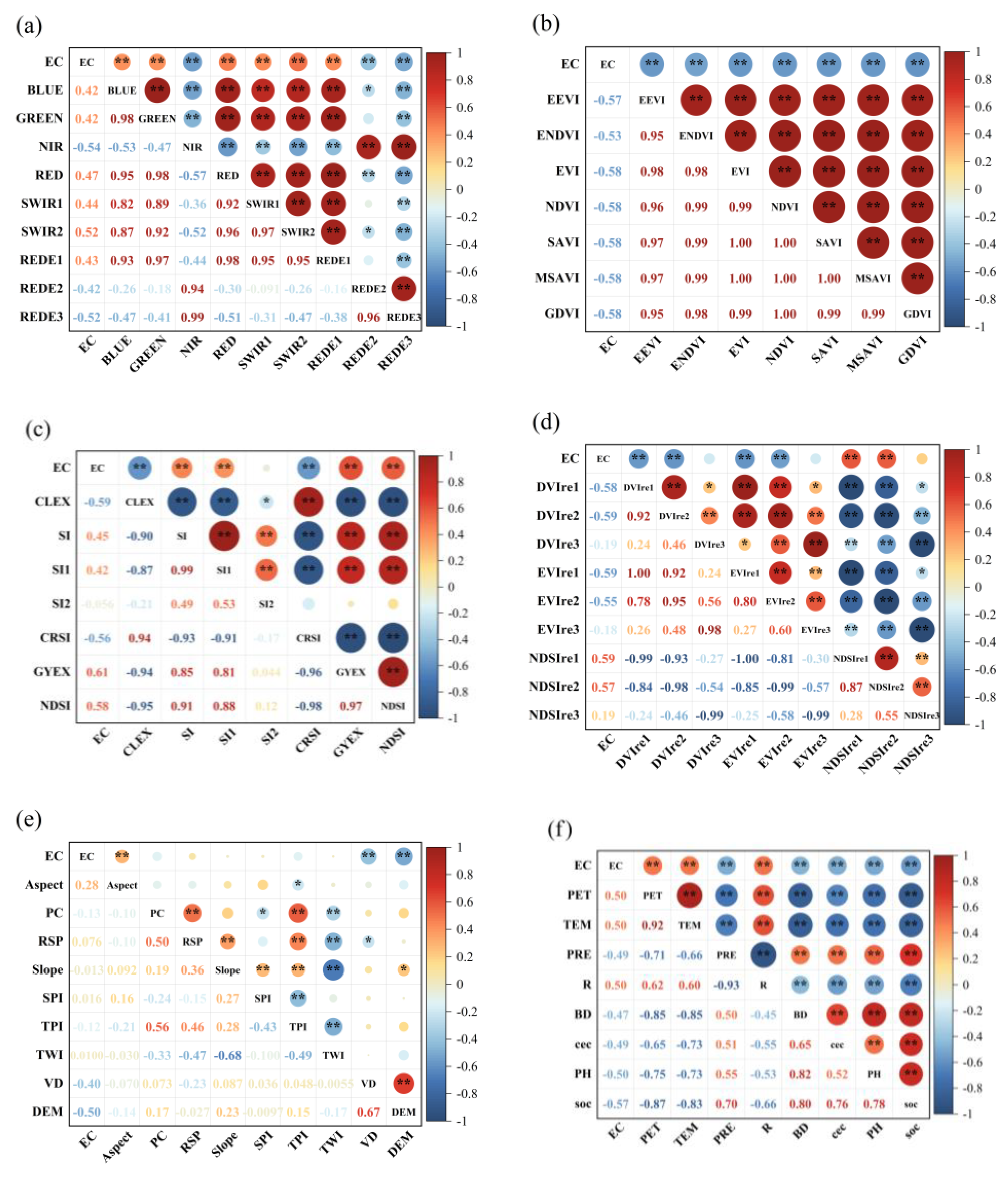
3.2. Correlation Analysis

Choosing environmental variables correlated with salinity for salinization monitoring can enhance modeling efficiency and accuracy to a certain degree. Thus, before variable selection in this study, we used Pearson correlation analysis as a pre-selection tool, firstly eliminating variables uncorrelated with electrical conductivity EC. The retained variables were used as candidate feature variables and optimized using two different feature selection methods. The Pearson correlation between soil electrical conductivity EC and the reflectance of nine Sentinel-2 spectral bands, along with 40 feature variables (seven vegetation indices, seven salinity indices, nine red-edge spectral indices, nine topographic indices, four meteorological indices, and four soil property indices), is depicted as follows. In Figure 4a, significant correlations exist between electrical conductivity and the near-infrared, short-wave infrared 2, and red-edge 3 bands among the nine bands, with correlation coefficients |r| > 0.5. Figure 4b reveals significant negative correlations for all seven vegetation indices due to minimal vegetation growth in soils with higher salinization. In Figure 4c, four out of the seven salinity indices demonstrate significant correlations, notably the GYEX index with a correlation coefficient of 0.61. Figure 4d presents that among the nine red-edge spectral indices, three indices were constructed, replacing red bands with red-edge bands, leading to a 0.1 increase in correlation coefficients for EVI and NDSI indices derived from red-edge band 1, while indices from red-edge band 3 show decreased correlation. In Figure 4e, only aspect, VD, and DEM among the nine topographic indices show correlation at p < 0.01; in Figure 4f, both meteorological and soil property indices correlate with EC. Notably, soil organic carbon exhibits the strongest negative correlation with soil salinity, with a coefficient of −0.57. Variables not correlated with EC are excluded, leaving 39 variables (nine bands, seven vegetation indices, six salinity indices, six red-edge band indices, three topographic indices, four meteorological indices, and four soil property indices) as candidates for future modeling.

3.3. Selection of Environmental Covariates and Bands

3.3.1. Results of Boruta-Based Feature Selection

Based on the Boruta algorithm’s variable selection outcome (Figure 5), 14 out of 39 candidate variables are identified as significant. EVI, DVI, and NDSI, developed from Red-Edge Band 2, are regarded as the most crucial characteristics. Soil properties such as pH value, soil organic carbon, and cation exchange capacity are also deemed important. Regarding salinity indices, CLEX and GYEX surpass the significance of the most substantial random shadow features. As for vegetation indices, only EEVI was chosen. Concerning meteorological indices, average monthly precipitation PRE and evapotranspiration PET are seen as significant. Regarding spectral bands, Red-Edge bands REDE2 and REDE3 are viewed as comparatively significant band variables. Nonetheless, terrain indices exert minimal influence on electrical conductivity EC, with only the slope Aspect identified as a crucial variable. In summary, relative to environmental covariates, the spectral band indices of S2 data hold more significance for soil EC values, particularly the Red-Edge band indices. This discovery further confirms the suitability of S2 spectral band indices in studies of soil salinity.

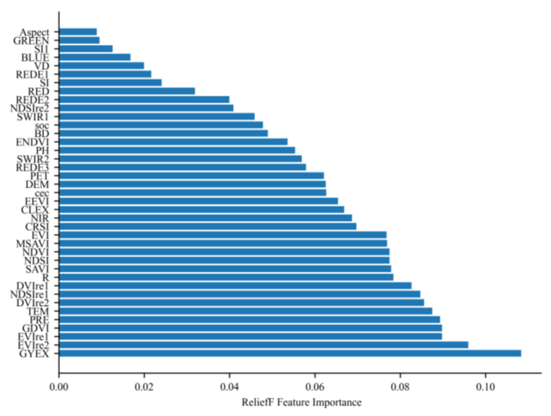
3.3.2. Results of ReliefF-Based Feature Selection

As depicted in Figure 6, the feature importance ranking based on the ReliefF algorithm shows feature weights varying between 0.01 and 0.12, with GYEX featuring the highest weight and slope Aspect the lowest. This paper identifies features with weights above the average weight (0.06) as significant, and those below 0.06 as insignificant, resulting in 22 variables being selected. Out of these, five indices from the Red-Edge bands were chosen, with 10 indices in vegetation and salinity deemed important. Regarding climate features, the weights of four indices exceed the average value. Within the soil property data, only the cation exchange capacity (cec) has been chosen.

3.4. Building and Validating the Soil Electrical Conductivity Inversion Model

Table 5. Mean values of evaluation indicators.

Modelling Strategy	Number of Independent Variables	Model	Average of Training Set			Average of Validation Set
			${\mathbf{R}}_{\mathbf{t}\mathbf{r}\mathbf{a}\mathbf{i}\mathbf{n}}^2$	${\mathbf{R}\mathbf{M}\mathbf{S}\mathbf{E}}_{\mathbf{t}\mathbf{r}\mathbf{a}\mathbf{i}\mathbf{n}}$	${\mathbf{M}\mathbf{A}\mathbf{E}}_{\mathbf{t}\mathbf{r}\mathbf{a}\mathbf{i}\mathbf{n}}$	${\mathbf{R}}_{\mathbf{t}\mathbf{e}\mathbf{s}\mathbf{t}}^2$	${\mathbf{R}\mathbf{M}\mathbf{S}\mathbf{E}}_{\mathbf{t}\mathbf{e}\mathbf{s}\mathbf{t}}$	${\mathbf{M}\mathbf{A}\mathbf{E}}_{\mathbf{t}\mathbf{e}\mathbf{s}\mathbf{t}}$
Strategy I	39	LightGBM	0.65	14.09	10.07	0.53	25.12	17.74
		SVM	0.48	19.49	13.45	0.38	26.16	18.93
		ELM	0.49	19.25	12.99	0.41	24.50	16.62
Strategy II	14	LightGBM	0.87	10.80	8.70	0.72	12.49	11.15
		SVM	0.56	22.04	16.36	0.43	20.29	15.57
		ELM	0.51	23.23	15.67	0.46	20.77	15.14
Strategy III	22	LightGBM	0.82	12.02	8.98	0.67	16.42	12.20
		SVM	0.49	23.66	17.63	0.47	19.42	14.44
		ELM	0.54	18.48	13.04	0.51	22.80	15.75

illustrates the mean predictive performance of three models based on various variable selection algorithms following ten-fold cross-validation. Strategy I represents three prediction models (LightGBM, SVM, and ELM) without any feature selection algorithm. Strategy II represents the combination of the Boruta feature selection algorithm and a prediction model (LightGBM, SVM, or ELM). Strategy III represents the combination of the ReliefF feature selection algorithm and a prediction model (LightGBM, SVM, or ELM). In the comparison of the validation set with LightGBM, ELM, and SVM modeling, Strategies II and III both outperformed Strategy I in model prediction, and Strategy II’s coefficients of determination $R^2$ were 0.72, 0.43, and 0.46, showing improvements of 33.96%, 26.32%, and 12.20%, respectively, compared to Strategy I. Strategy III’s coefficients of determination $R^2$, in comparison to Strategy I, demonstrate increases of 26.42%, 13.16%, and 26.83%. This suggests that the estimation accuracy and stability of the model have improved to varying extents after correction with algorithm-selected variables.

Compared with ReliefF, Boruta is applicable to a wider range of data types, and not only considers the importance of a single feature but also the interaction between features. Therefore, it can evaluate the importance of features more accurately, and it is more robust when dealing with data with a large number of features and noises. However, it is sensitive to superparameters. As for LightGBM, it has better feature selection ability, faster training speed, and higher accuracy when compared with ELM and SVM, especially for large-scale and high-dimensional land data, but parameter tuning is more complicated and sensitive to outliers. In order to give full play to their respective advantages, Boruta and LightGBM are combined into a Boruta-LightGBM strategy and applied to feature selection and soil conductivity prediction. The accuracy validation results reveal that LightGBM exhibited the most optimal predictive performance across all three strategies, with Boruta-LightGBM modeling attaining the highest $R^2$ and the lowest RMSE and MAE (${\mathrm{R}}_{\mathrm{t}\mathrm{e}\mathrm{s}\mathrm{t}}^2=0.72$, ${\mathrm{R}\mathrm{M}\mathrm{S}\mathrm{E}}_{\mathrm{t}\mathrm{e}\mathrm{s}\mathrm{t}}=12.49$, ${\mathrm{M}\mathrm{A}\mathrm{E}}_{\mathrm{t}\mathrm{e}\mathrm{s}\mathrm{t}}=11.15$) for superior performance. The scatter plot depicting its optimal fit line is illustrated in Figure 7.

Across the three strategies, the SVM model demonstrates weaker overall predictive capability, with its ${\mathrm{R}}_{\mathrm{t}\mathrm{e}\mathrm{s}\mathrm{t}}^2$ never surpassing 0.5 and remaining the lowest compared to the $R^2$ of the other models. ReliefF’s selection outcomes prove more apt for the SVM and ELM models than Boruta’s, showing enhancements in both ${\mathrm{R}}_{\mathrm{t}\mathrm{r}\mathrm{a}\mathrm{i}\mathrm{n}}^2$ and ${\mathrm{R}}_{\mathrm{t}\mathrm{e}\mathrm{s}\mathrm{t}}^2$. The disparity between ${\mathrm{R}}_{\mathrm{t}\mathrm{r}\mathrm{a}\mathrm{i}\mathrm{n}}^2$ and ${\mathrm{R}}_{\mathrm{t}\mathrm{e}\mathrm{s}\mathrm{t}}^2$ for ReliefF-SVM and ReliefF-ELM is within 0.03, signifying the strong generalization capacity of the models, yet their overall predictive ability falls short of the anticipated level (${\mathrm{R}}_{\mathrm{t}\mathrm{e}\mathrm{s}\mathrm{t}}^2$ > 0.6). The mean values of the evaluation metrics across 100 trials of the average model are presented in Table 5.

3.5. Soil EC Mapping

Owing to the optimal outcomes of the Boruta-LightGBM model, this research employs the mean soil electrical conductivity results from 100 iterations of the Boruta-LightGBM model as the basis for the predicted salinity distribution map in the study area (Figure 8). As per the United States Department of Agriculture (USDA) standards for various soil salinity levels, soil salinity can be categorized into five classes: I Non-saline soil (EC < 2 ds/m), II Mild salinization (2 ds/m ≤ EC < 4 ds/m), III Moderate salinization (4 ds/m ≤ EC < 8 ds/m), IV Severe salinization (8 ds/m ≤ EC < 16 ds/m), and V Saline soil (EC ≥ 16 ds/m). The conductivity distribution map produced for the study area is depicted as follows: the predicted range of conductivity in the study area (0.23 ds/m ≤ EC ≤ 89.07 ds/m) aligns largely with our actual measured data range. The respective proportions of non-saline soil, mildly salinized, moderately salinized, severely salinized, and saline soil are 37%, 19%, 13%, 20%, and 11%.

As indicated by the map, the oasis’s interior mainly consists of non-salinized and mildly salinized areas, while moderately and severely salinized soils are predominantly located along the oasis’s periphery, encompassing regions near the downstream ends of the Kuqa and Ogan Rivers. Soil salinity escalates from the northwest to the southeast of the oasis. This is attributed to the high vegetation cover within the oasis, which likely reduces intense evaporation during water infiltration, preventing excessive salt accumulation. The southeast portion is predominantly desert, characterized by an arid climate, limited precipitation, and strong evaporation. As saline groundwater reaches the surface due to evaporation, salts accumulate, leading to high salinity in desert soils. Moreover, certain desert plants possess salt-accumulating capabilities, further elevating soil salinity levels. The spatial distribution of salinity in the study area, as predicted by the model, aligns with the results of our field surveys.

3.6. The Influence of Temporal-Spatial Variability on Environmental Factors

Multicollinearity testing of environmental variables was performed with IBM SPSS Statistics 26. The results, detailed in

Table 6. Multicollinearity testing of environmental variables.

Environmental Variables	Multicollinearity Testing
	Tolerance	VIF
soc	0.265	3.780
PRE	0.617	1.621
PH	0.191	5.228
cec	0.124	8.067
TEM	0.135	7.388
SPI	0.569	1.757

, reveal that six out of seventeen environmental variables are free from multicollinearity, adhering to the criteria of VIF < 10 and a tolerance above 0.1. Utilizing soil electrical conductivity EC as the dependent variable and the six multicollinearity-tested variables as independent variables, the MGWR model was developed using the MGWR2.2 software. The statistical results for the regression coefficients of the MGWR model can be found in

Table 7. The statistical results for the regression coefficients of the MGWR model.

Variables	Bandwidth	Mean	SD	Min	Median	Max
Intercept	32	−0.139	0.011	−0.158	−0.142	−0.120
soc	87	−0.339	0.029	−0.381	−0.312	−0.297
PRE	91	−0.228	0.016	−0.255	−0.239	−0.201
PH	65	0.034	0.251	−1.459	0.640	1.527
cec	85	−0.312	0.017	−2.653	−0.177	2.637
TEM	85	−0.307	0.019	−0.335	−0.306	−0.276
SPI	65	−0.173	0.129	−2.829	−0.770	1.167

. In practical scenarios, as environmental factors differ across geographic locations, the relationship between soil electrical conductivity (EC) and these factors also varies, indicating temporal-spatial heterogeneity. The MGWR model utilizes varying spatial scales for different environmental variables, enabling local estimation of regression parameters for independent variables at each spatial location during spatial prediction [37]. With a global bandwidth of 94 samples, factors such as cec, PRE, soc, and TEM, having smaller standard deviations in their regression coefficients, suggest that these environmental variables tend to impact soil electrical conductivity EC at a global level. PH and SPI have smaller bandwidths, indicating a more pronounced temporal-spatial heterogeneity in their effect on soil electrical conductivity EC. Based on the average and median absolute values of the regression coefficients for environmental factors, soc, PRE, PH, and TEM significantly influence the spatial distribution of soil electrical conductivity EC in the study area. The subsequent section will detail the spatial variability of environmental factors on soil electrical conductivity EC, focusing on the distribution of each factor’s regression coefficients (Figure 7).

In Figure 9A, the regression coefficients for average monthly temperature vary from −1.252 to 1.575. The spatial pattern, judging by the absolute values of these coefficients, shows higher values in the west and lower in the east, signifying that temperature influences soil salinity more in the western region of the study area than in the eastern region. The western part is mainly an oasis agricultural zone, replete with extensive farmlands and landscape vegetation. Rising temperatures can modify the dynamics of soil moisture and the migration patterns of salts in the soil. With the upward evaporation of soil moisture, dissolved salts are transported to the soil surface with the moisture and settle on the surface after the moisture evaporates, resulting in the accumulation of salts in the topsoil.

In Figure 9B, the regression coefficients of soil organic carbon (soc) lie between −2.826 and 1.167. Considering the absolute values of these coefficients, the overall impact exhibits a spatial pattern of decreasing influence from the inner to the outer parts of the oasis. In the southwest area, soil organic carbon demonstrates a pronounced negative influence on soil salinity. This is due to the high vegetation cover in the southwestern section of the study area. Previous studies indicate a positive correlation between vegetation cover and topsoil organic carbon content. Thus, the high organic carbon content in the southwest leads to improved soil water retention and permeability, potentially aiding in the dissolution, movement, and absorption of soil salts, which in turn reduces soil salinity.

In Figure 9C, soil pH regression coefficients range from −1.459 to 1.527, showing a spatial pattern with higher values in the west and lower in the east. The positive impact is mainly in the western region of the study area, dominated by agricultural lands within the oasis, where soil pH is altered by agricultural irrigation and fertilization activities. The regression coefficients for pH values in the eastern region of the study area are negative, suggesting a substantial negative effect of pH on soil salinity. Lower pH values correlate with increased soil salinity. Moreover, rising soil salinity levels contribute to soil acidification, as the decomposition of salt substances releases hydrogen and other acidic ions, further acidifying the soil.

In Figure 9D, the range of regression coefficients for average monthly precipitation (PRE) is between −1.285 and 2.115. The spatial pattern, as inferred from the absolute values of the coefficients, reveals higher values in the west and lower in the east. The eastern region of the study area experiences limited precipitation, and the desert areas, characterized by sparse or absent vegetation, lack the regulatory role of plants in soil moisture and salinity. Consequently, the impact of precipitation on soil salinity in desert regions is relatively limited. The regression coefficients are greatest at the junction between the oasis and the desert, an area often representing an ecological transition zone, where water dynamics are more intricate than in solely desert regions. In these zones, precipitation can interact with irrigation water, resulting in the redistribution of salts within the soil profile, thereby exerting a more significant influence on soil salinity.

In Figure 9E, the regression coefficients for cation exchange capacity (CEC) lie between −0.265 and 2.636, with both mean and median values being negative. This suggests a pronounced negative influence of cation exchange capacity on soil salinity in the study area’s northwest. In this region, high levels of cation exchange capacity contribute to cations being adsorbed onto soil colloids via electrostatic forces, thereby mitigating excessive salt concentration in the soil solution.

In Figure 9F, the regression coefficients of the stream power index range between −2.826 and 1.167. These coefficients show a negative influence in the western section of the study area, encompassing the region west of the southern tip of the middle Ogan-Kuqa River, a glacial meltwater stream. This area features a higher runoff dynamic index, with the topography declining from north to south. An increased runoff dynamic index suggests a more pronounced downward movement of water and solutes in the soil, which could result in decreased soil salinity.

4. Discussion

Feature selection aims to minimize the dimensionality of features to improve model performance and interpretability. Traditional feature variable selection methods predominantly use Pearson correlation analysis. While Pearson’s correlation coefficient can assess the linear relationship between two variables, it falls short of accurately representing nonlinear relationships [44]. Hence, there is a need to refine existing methods to more thoroughly investigate and comprehend the intricate relationships between soil feature variables. Consequently, in our research, we employed Pearson correlation analysis as an initial approach to exclude variables not significantly correlated with soil electrical conductivity (EC). We then utilized the Boruta and ReliefF algorithms for modeling tests, effectively reducing input data redundancy in the soil electrical conductivity (EC) prediction model and analyzing the influence of crucial variables specific to various data sources. This optimization approach improves our interpretation and understanding of the model outcomes, enabling precise evaluations of how different variable selection methods affect model prediction accuracy and therefore strongly supporting model performance optimization. Research findings show that, in comparison to models built solely on variables selected through Pearson correlation analysis, the optimal variables further filtered by the Boruta and ReliefF algorithms notably increase the model’s accuracy. In our research, upon comparing modeling strategies involving varying numbers of input variables, the Boruta-LightGBM approach emerged as the most effective, improving the determination coefficient $R^2$ by 0.04 to 0.33 and decreasing the RMSE by 0.93 to 10.67, which is in line with Ge’s research findings [6]. The Boruta algorithm’s strength lies in its ability to detect correlations among features, thereby eliminating redundant information and revealing potential hidden features in the dataset. Moreover, the Boruta algorithm further effectively filters out noise features by generating random shadow features.

From analyzing the importance of variables in feature selection, it is evident that:

(1)

Red-edge band indices, calculated by substituting original red bands, are more sensitive to salinity compared to vegetation indices derived from the original red bands. These red-edge indices are frequently identified as important variables in both selection algorithms, likely related to potential spectral information and a higher signal-to-noise ratio in the red-edge region [24].

(2)

In predicting salinity, terrain indices rank lowest in relevance and importance. Only the aspect (Aspect) has a positive correlation with soil electrical conductivity (EC) and meets the criterion for an important variable in both selection methods. This is due to the study area’s relatively flat topography, which does not effectively correlate with the spatio-temporal distribution of soil salinity [45]. Aspect influences salinization mainly through changes in sunlight exposure, with sunny slopes having longer sunlight exposure and higher soil moisture evaporation than shady slopes, thus enhancing soil salinization. Yet, this factor also requires consideration of seasonal changes and vegetation coverage [46].

(3)

In both feature selection methods, soil organic carbon (SOC) and cation exchange capacity (CEC) emerge as significant. Soil organic carbon (SOC), part of soil organic matter, supplies plant nutrients and augments the soil’s capacity to adsorb cations (such as Na⁺, Ca²⁺, etc.) [47]. The cation exchange capacity (CEC) of soil is the number of cations that soil colloids can adsorb on their surfaces. Therefore, when the soil colloids’ capacity to adsorb cations increases, the soil’s salinity content decreases. Variations in soil cation exchange capacity (CEC) impact the pH and electrical conductivity of soil moisture, which in turn affects the adsorption and desorption of ions in the soil, further influencing soil salinity content.

Soil salinity is influenced by multiple environmental factors, such as climate, rainfall, and soil types. The degree of soil salinization often varies with spatial changes, showing significant temporal-spatial heterogeneity in the relationship between environmental factors and soil salinity. Traditional global regression models such as PLSR, MLR, and BPNN treat the relationship between independent and dependent variables as constant, overlooking the variations caused by spatial variability [48]. The MGWR model takes into account the differential impact scales of various environmental factors, enabling the identification of the geographic processes through which each variable affects the dependent variable across different spatial scales [49]. Therefore, this study employs the MGWR model’s independent variable regression coefficients to explore the temporal-temporal-spatial heterogeneity in how environmental factors affect soil electrical conductivity (EC). Examining the soil electrical conductivity (EC) results predicted by the MGWR model (Figure 10), the study area exhibits a gradual increase in salinity from northwest to southeast, aligning with the spatial distribution of salinity mapping in Section 3.4. The MGWR model’s simulation accuracy, reflected in the determination coefficient $R^2$ of 0.519 and information criterion indices AIC = 233.386 and AICc = 242.201, shows an improvement over global regression results ($R^2$ = 0.386, AIC=238.962, AICc = 243.613). The $R^2$ value increased by 0.133, and the information criterion indices decreased by 5.576 and 1.412, respectively, indicating better model performance with lower indices. The MGWR model’s multi-scale feature effectively captures the impact of various environmental covariates on the dependent variable across different spatial scales [50]. This multi-scale capability enhances the model’s predictive strength and allocates distinct spatial bandwidths to the spatial impacts of different environmental covariates, accurately interpreting the characteristics exhibited by these covariates at diverse scales.

5. Conclusions

In this research, six environmental covariates were selected: vegetation indices, salinity indices, Red-Edge band indices, meteorological factors, terrain indices, and soil property data. First, the correlation of each environmental covariate with soil electrical conductivity (EC) was analyzed using Pearson correlation coefficients. Subsequently, the Boruta and ReliefF algorithms were employed for variable selection, and vital variables were selected based on their importance ranking for input into the LightGBM, ELM, and SVM models for modeling soil electrical conductivity (EC) as both independent and dependent variables. Based on the optimally performing model, maps of soil electrical conductivity (EC) were produced in the study region. Ultimately, the MGWR model was used to explore the temporal-spatial heterogeneity in the impact of environmental factors on soil electrical conductivity (EC). The conclusions are as follows:

(1)

Conducting variable selection before building soil salinity inversion models enhances model performance and prediction accuracy, efficiently reduces data dimensions, and thus helps identify the key variables most impacting the target variable, leading to a deeper understanding of the data–model relationship. Among six environmental covariates, Red-Edge band indices hold the highest importance, and terrain indices the least.

(2)

With varying numbers of input variables in the model, the modeling strategy based on Boruta-LightGBM exhibits optimal performance, accounting for 65% to 77% of the spatio-temporal variation in soil electrical conductivity (EC).

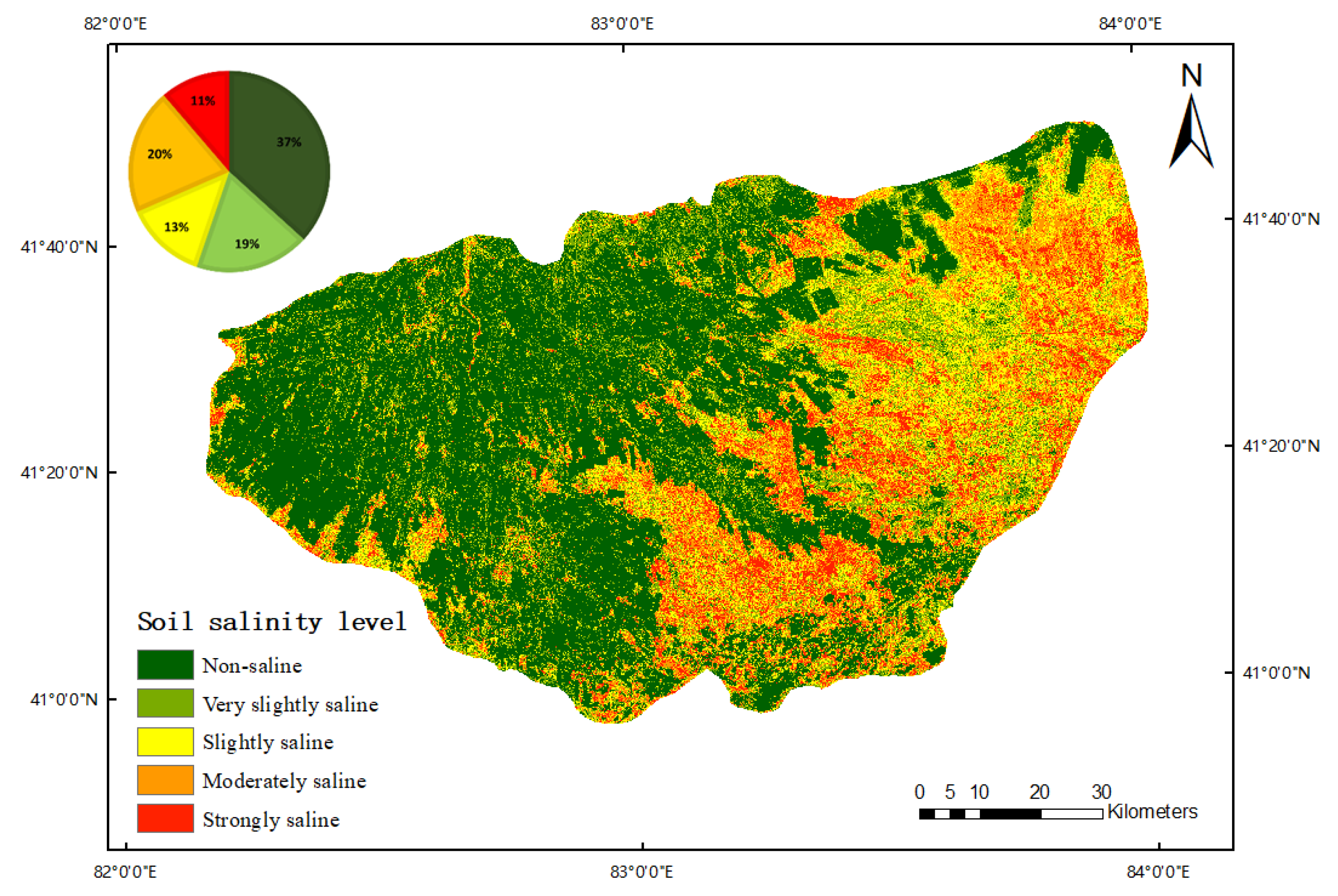
(3)

In the study area, soil salinity exhibits a trend of gradually increasing from northwest to southeast. The respective proportions of non-saline soil, light salinization, moderate salinization, severe salinization, and saline soil are 37%, 19%, 13%, 20%, and 11%.

(4)

MGWR findings show that soc, PRE, PH, and TEM significantly impact soil electrical conductivity (EC) in the study area and exhibit notable spatio-temporal differences. In the Ogan-Kuqa River basin area of the study, the Stream Power Index (SPI) significantly affects soil electrical conductivity (EC), and within the oases, the cation exchange capacity (cec) exerts a strong negative influence on soil electrical conductivity (EC).

References

1. Zinck, G.I.M.A. Remote sensing of soil salinity: Potentials and constraints. Remote Sens. Environ. 2003, 25, 1–20. [Google Scholar]
2. Weng, B.; Zheng, X. Thinking and Countermeasures for Rational Utilization of Soil Fertility in Modern Agriculture Developping. J. Agric. Resour. Environ. 2014, 405, 1875. [Google Scholar]
3. Ivushkin, K.; Bartholomeus, H.; Bregt, A.K.; Pulatov, A.; Sousa, L.D. Global mapping of soil salinity change. Remote Sens. Environ. 2019, 231, 111260. [Google Scholar] [CrossRef]
4. An, D.; Zhao, G.; Chang, C.; Wang, Z.; Li, P.; Zhang, T.; Jia, J. Hyperspectral field estimation and remote-sensing inversion of salt content in coastal saline soils of the Yellow River Delta. Int. J. Remote Sens. 2016, 37, 455–470. [Google Scholar] [CrossRef]
5. Nwer, B.; Zurqani, H.; Rhoma, E. The Use of Remote Sensing and Geographic Information System for Soil Salinity Monitoring in Libya. GSTF J. Geol. Sci. 2013, 1, 38–42. [Google Scholar] [CrossRef] [PubMed]
6. Ge, X.; Ding, J.; Teng, D.; Wang, J.; Huo, T.; Jin, X.; He, B.; Han, L. Updated soil salinity with fine spatial resolution and high accuracy: The synergy of Sentinel-2 MSI, environmental covariates and hybrid machine learning approaches. Catena Interdiscip. J. Soil Sci. Hydrol.-Geomorphol. Focus. Geoecology Landsc. Evol. 2022, 212, 106054. [Google Scholar] [CrossRef]
7. Ijaz, Z.; Zhao, C.; Ijaz, N.; Rehman, Z.U.; Ijaz, A. Novel application of Google earth engine interpolation algorithm for the development of geotechnical soil maps: A case study of mega-district. Geocarto Int. 2022, 37, 18196–18216. [Google Scholar] [CrossRef]
8. Ijaz, Z.; Zhao, C.; Ijaz, N.; Rehman, Z.U.; Ijaz, A. Spatial mapping of geotechnical soil properties at multiple depths in Sialkot region, Pakistan. Environ. Earth Sci. 2021, 80, 787. [Google Scholar] [CrossRef]
9. Shi, T.; Wang, J.; Liu, H.; Chen, Y.; Wu, G. Soil Organic Carbon Content Estimation with Laboratory-Based Visible-Near-Infrared Reflectance Spectroscopy: Feature Selection. Appl. Spectrosc. Soc. Appl. Spectrosc. 2014, 68, 831–837. [Google Scholar] [CrossRef] [PubMed]
10. Taghizadeh-Mehrjardi, R.; Minasny, B.; Sarmadian, F.; Malone, B.P. Digital mapping of soil salinity in Ardakan region, central Iran. Geoderma 2014, 213, 15–28. [Google Scholar] [CrossRef]
11. Qian, Z.; Jianli, D.; Xiangyu, G.; Ke, L.; Zipeng, Z.; Yongsheng, G. Estimation of soil organic matter in the Ogan-Kuqa River Oasis, Northwest China, based on visible and near-infrared spectroscopy and machine learning. J. Arid Land 2023, 15, 191–204. [Google Scholar]
12. Luo, C.; Zhang, X.; Wang, Y.; Men, Z.; Liu, H. Regional soil organic matter mapping models based on the optimal time window, feature selection algorithm and Google Earth Engine. Soil Tillage Res. 2022, 219, 105325. [Google Scholar] [CrossRef]
13. Mohamed, S.A.; Metwaly, M.M.; Metwalli, M.R.; AbdelRahman, M.A.; Badreldin, N. Integrating Active and Passive Remote Sensing Data for Mapping Soil Salinity Using Machine Learning and Feature Selection Approaches in Arid Regions. Remote Sens. 2023, 15, 1751. [Google Scholar] [CrossRef]
14. Wang, Y.; Xie, M.; Hu, B.; Jiang, Q.; Shi, Z.; He, Y.; Peng, J. Desert Soil Salinity Inversion Models Based on Field In Situ Spectroscopy in Southern Xinjiang, China. Remote Sens. 2022, 14, 4962. [Google Scholar] [CrossRef]
15. Xinsheng, Z.; Baoshan, C.; Tao, S. The relationship between the spatial distribution of vegetation and soil environmental factors in the tidal creek areas of the Yellow River Delta. Ecol. Environ. Sci. 2010, 19, 1855–1861. [Google Scholar]
16. Matteo, P.; Silvia, C.; Giancarlo, P.; Michele, P. Modelling and mapping Soil Organic Carbon in annual cropland under different farm management systems in the Apulia region of Southern Italy. Soil Tillage Res. 2024, 235, 105916. [Google Scholar]
17. Zhang, Y.; Wang, Y.; Bai, Y.; Zhang, R.; Liu, X.; Ma, X. Prediction of Spatial Distribution of Soil Organic Carbon in Helan Farmland Based on Different Prediction Models. Land 2023, 12, 1984. [Google Scholar] [CrossRef]
18. Ye, H.; Huang, W.; Huang, S.; Huang, Y.; Zhang, S.; Dong, Y.; Chen, P. Effects of different sampling densities on geographically weighted regression kriging for predicting soil organic carbon. Spat. Stat. 2017, 20, 76–91. [Google Scholar] [CrossRef]
19. Hojjatollah, M.; Alireza, S.; Babak, M. Improving groundwater nitrate concentration prediction using local ensemble of machine learning models. J. Environ. Manag. 2023, 345, 118782. [Google Scholar]
20. Jiang, Z.; Xu, B. Geographically weighted regression analysis of the spatially varying relationship between farming viability and contributing factors in Ohio. Reg. Sci. Policy Pract. 2014, 6, 69–83. [Google Scholar] [CrossRef]
21. Fotheringham, A.S.; Yang, W.; Kang, W. Multiscale Geographically Weighted Regression (MGWR). Ann. Am. Assoc. Geogr. 2017, 107, 1247–1265. [Google Scholar] [CrossRef]
22. Liu, F.; Wu, H.; Zhao, Y.; Li, D.; Yang, J.L.; Song, X.; Shi, Z.; Zhu, A.X.; Zhang, G.L. Mapping high resolution National Soil Information Grids of China. Sci. Bull. 2022, 67, 328–340. [Google Scholar] [CrossRef] [PubMed]
23. Guolin, M.A.; Jianli, D.; Lijing, H.; Zipeng, Z.; Si, R. Digital mapping of soil salinization based on Sentinel-1 and Sentinel-2 data combined with machine learning algorithms. Reg. Sustain. 2021, 2, 177–188. [Google Scholar]
24. Wang, J.; Ding, J.; Yu, D.; Ma, X.; Yu, D. Capability of Sentinel-2 MSI data for monitoring and mapping of soil salinity in dry and wet seasons in the Ebinur Lake region, Xinjiang, China. Geoderma 2019, 353, 172–187. [Google Scholar] [CrossRef]
25. Ma, S.; He, B.; Xie, B.; Ge, X.; Han, L. Investigation of the spatial and temporal variation of soil salinity using Google Earth Engine: A case study at Werigan–Kuqa Oasis, West China. Sci. Rep. 2023, 13, 2754. [Google Scholar] [CrossRef] [PubMed]
26. Tian, Y.C.; Yao, X.; Yang, J.; Cao, W.X.; Hannaway, D.B.; Zhu, Y. Assessing newly developed and published vegetation indices for estimating rice leaf nitrogen concentration with ground- and space-based hyperspectral reflectance. Field Crops Res. 2011, 120, 299–310. [Google Scholar] [CrossRef]
27. Peng, S.; Ding, Y.; Liu, W.; Zhi, L.I. 1 km monthly temperature and precipitation dataset for China from 1901 to 2017. Earth Syst. Sci. Data 2019, 11, 1931–1946. [Google Scholar] [CrossRef]
28. Peng, S.; Ding, Y.; Wen, Z.; Chen, Y.; Cao, Y.; Ren, J. Spatiotemporal change and trend analysis of potential evapotranspiration over the Loess Plateau of China during 2011–2100. Agric. For. Meteorol. 2017, 233, 183–194. [Google Scholar] [CrossRef]
29. Kursa, M.B.; Rudnicki, W.R. Feature Selection with Boruta Package. J. Stat. Softw. 2010, 36, 1–13. [Google Scholar] [CrossRef]
30. Gan, W.; Zhang, Y.; Xu, J.; Yang, R.; Xiao, A.; Hu, X. Spatial Distribution of Soil Heavy Metal Concentrations in Road-Neighboring Areas Using UAV-Based Hyperspectral Remote Sensing and GIS Technology. Sustainability 2023, 15, 10043. [Google Scholar] [CrossRef]
31. Lawal, I.M.; Bertram, D.; White, C.J.; Kutty, S.R.M.; Hassan, I.; Jagaba, A.H. Application of Boruta algorithms as a robust methodology for performance evaluation of CMIP6 general circulation models for hydro-climatic studies. Theor. Appl. Climatol. 2023, 153, 113–135. [Google Scholar] [CrossRef]
32. Kira, K.; Rendell, L.A. A Practical Approach to Feature Selection; Morgan Kaufmann Publishers Inc.: Cambridge, MA, USA, 1992. [Google Scholar]
33. Xie, S.; Li, K.; Xiao, M.; Zhang, L.; Li, W. Key Quality Indicators Prediction for Web Browsing with Embedded Filter Feature Selection. Appl. Sci. 2020, 10, 2141. [Google Scholar] [CrossRef]
34. Mahsa, H.; Abbas, M.; Reza, G. A Novel Scheme for Mapping of MVT-Type Pb–Zn Prospectivity: LightGBM, a Highly Efficient Gradient Boosting Decision Tree Machine Learning Algorithm. Nat. Resour. Res. 2023, 32, 2417–2438. [Google Scholar]
35. Junting, Z.; Xiaoye, Z.; Ke, G.; Yaqiang, W.; Huizheng, C.; Xiaojing, S.; Lei, Z.; Yangmei, Z.; Junying, S.; Wenjie, Z. Robust prediction of hourly PM2.5 from meteorological data using LightGBM. Natl. Sci. Rev. 2021, 8, nwaa307. [Google Scholar]
36. Jafar, A.; Golshan, M. Machine learning approaches for predicting arsenic adsorption from water using porous metal–organic frameworks. Sci. Rep. 2022, 12, 16458. [Google Scholar]
37. Huang, G.B.; Zhou, H.; Ding, X.; Zhang, R. Extreme Learning Machine for Regression and Multiclass Classification. IEEE Trans. Syst. Man Cybern. Part B Cybern. 2012, 42, 513–529. [Google Scholar] [CrossRef] [PubMed]
38. Yadav, B.; Ch, S.; Mathur, S.; Adamowski, J. Estimation of in-situ bioremediation system cost using a hybrid Extreme Learning Machine (ELM)-particle swarm optimization approach. J. Hydrol. 2016, 543, 373–385. [Google Scholar] [CrossRef]
39. Kang, X.; Zhao, Y.; Li, J. Predicting refractive index of ionic liquids based on the extreme learning machine (ELM) intelligence algorithm. J. Mol. Liq. 2018, 250, 44–49. [Google Scholar] [CrossRef]
40. Cortes, C.; Vapnik, V. Support-Vector Networks. Mach. Learn. 1995, 20, 273–297. [Google Scholar] [CrossRef]
41. Ilyas, N.; Vasit, S.; Li, D.J.; Ümüt, H.; Abdulla, A.; Zaytungul, Y. A WFS-SVM Model for Soil Salinity Mapping in Keriya Oasis, Northwestern China Using Polarimetric Decomposition and Fully PolSAR Data. Remote Sens. 2018, 10, 598. [Google Scholar]
42. Yang, S.H.; Liu, F.; Song, X.D.; Lu, Y.Y.; Li, D.C.; Zhao, Y.G.; Zhang, G.L. Mapping topsoil electrical conductivity by a mixed geographically weighted regression kriging: A case study in the Heihe River Basin, northwest China. Ecol. Indic. 2019, 102, 252–264. [Google Scholar] [CrossRef]
43. Yuting, Z.; Kai, H.; Hui, Q.; Yanyan, G.; Yuan, F.; Shan, X.; Shunqi, T.; Qiying, Z.; Wengang, Q.; Wenhao, R. Characterization of soil salinization and its driving factors in a typical irrigation area of Northwest China. Sci. Total Environ. 2022, 837, 155808. [Google Scholar]
44. Wang, J.; Shi, T.; Yu, D.; Teng, D.; Ge, X.; Zhang, Z.; Yang, X.; Wang, H.; Wu, G. Ensemble machine-learning-based framework for estimating total nitrogen concentration in water using drone-borne hyperspectral imagery of emergent plants: A case study in an arid oasis, NW China. Environ. Pollut. 2020, 266, 115412. [Google Scholar] [CrossRef] [PubMed]
45. Phogat, V.; Pitt, T.; Petrie, P.; Šimůnek, J.; Cutting, M. Optimization of Irrigation of Wine Grapes with Brackish Water for Managing Soil Salinization. Land 2023, 12, 1947. [Google Scholar] [CrossRef]
46. Mahdi, T.M.; Mahdi, H. Developing geographic weighted regression (GWR) technique for monitoring soil salinity using sentinel-2 multispectral imagery. Environ. Earth Sci. 2021, 80, 75. [Google Scholar]
47. Salcedo, F.P.; Cutillas, P.P.; Cabañero, J.J.A.; Vivaldi, A.G. Use of remote sensing to evaluate the effects of environmental factors on soil salinity in a semi-arid area. Sci. Total Environ. 2021, 815, 152524. [Google Scholar] [CrossRef] [PubMed]
48. Nazeer, M.; Bilal, M. Evaluation of Ordinary Least Square (OLS) and Geographically Weighted Regression (GWR) for Water Quality Monitoring: A Case Study for the Estimation of Salinity. J. Ocean Univ. China 2018, 17, 305–310. [Google Scholar] [CrossRef]
49. Zeng, C.; Yang, L.; Zhu, A.-X.; Rossiter, D.G.; Liu, J.; Liu, J.; Qin, C.; Wang, D. Mapping soil organic matter concentration at different scales using a mixed geographically weighted regression method. Geoderma 2016, 281, 69–82. [Google Scholar] [CrossRef]
50. Shuangyin, Z.; Yiyun, C.; Zheyue, Z.; Siying, W.; Zihao, W.; Yongsheng, H.; Yan, W.; Haobo, H.; Zhongzheng, H.; Teng, F. VNIR estimation of heavy metals concentrations in suburban soil with multi-scale geographically weighted regression. Catena 2022, 219, 106585. [Google Scholar]
Figure 1. The workflow of this research.
Sustainability 16 02706 g001
Figure 2. Overview Map of the Study Area: (a) the study area in Xinjiang of China; (b) the river distribution of Kuqa-Ogan oasis.
Sustainability 16 02706 g002
Figure 3. Locations of the sampling sites in the Ogan-Kuqa River Oasis.
Sustainability 16 02706 g003
Figure 4. Correlation coefficients between electrical conductivity (EC) and Sentinel-2 multi-spectral bands (a), between EC and vegetation indices (b), between EC and salinity indices (c), between EC and red-edge band indices (d), between EC and topographic indices (e), and between EC and meteorological and soil property indices (f). Symbols ‘**’ denote significance at the p < 0.01 probability level, while ‘*’ indicates significance at the p < 0.05 probability level.
Sustainability 16 02706 g004
Figure 5. Importance of environmental covariates and bands determined by Boruta. Blue represents shadow features, green represents important features, and red represents unimportant features. Black rhombus represents the outlier.
Sustainability 16 02706 g005
Figure 6. Feature Weighting According to the ReliefF Algorithm.
Sustainability 16 02706 g006
Figure 7. Measured and predicted regression analysis of Boruta-LightGBM modeling.
Sustainability 16 02706 g007
Figure 8. Digital soil EC mapping driven by the Boruta-LightGBM Modelling strategy.
Sustainability 16 02706 g008
Figure 9. Distribution of MGWR regression coefficients.
Sustainability 16 02706 g009aSustainability 16 02706 g009b
Figure 10. Results of the MGWR model’s prediction of soil electrical conductivity (EC).
Sustainability 16 02706 g010